Hamiltonian Dynamics of the Protein Chain and Normal Modes of $\alpha$-Helix and $\beta$-Sheet

Abstract

We use the torsional angles of the protein chain as generalized coordinates in the canonical formalism, derive canonical equations of motion, and investigate the coordinate dependence of the kinetic energy expressed in terms of the canonical momenta. We use the formalism to compute the normal-frequency distributions of the $\alpha$-helix and the $\beta$-sheet, under the assumption that they are stabilized purely through hydrogen bonding. Comparison of their free energies show the existence of a phase transition between the $\alpha$-helix and the $\beta$-sheet at a critical temperature.

1 Introduction and results

The purpose of this work is to describe the backbone chain of a protein molecule in terms of dynamically independent variables, which are the torsional angles between successive units of the chain. These angles determined the average conformation of the chain, and local vibrations of chemical bonds only contribute to small fluctuations about the average. By ignoring these fluctuations, we gain a better overview of the motion of the chain, in particular its folding.

We use the torsional angles as generalized coordinates in the canonical formalism, with concomitant canonical momenta. The kinetic energy then becomes a function of the coordinates, when expressed in term of the canonical momenta. That is, masses are replaced by a generalized mass matrix, which is a function of the coordinates. There arises an effective potential, which is discussed in detailed later. By studying this mass matrix numerically, we find that the effective potential is approximately constant for almost all conformations of the chain. This result is significant for practical applications, particularly for the CSAW (conditioned self-avoiding walk) model [1, 2], where such an approach was first used.

Using the canonical formalism, we formulate the eigenvalue problem that describes the normal modes of the system with respect to an equilibrium conformation. Actual computations are carried out for a pure $\alpha$-helix and a pure $\beta$-sheet, to obtain distribution functions of the normal frequencies. These pure structures are hypothetical, of course, for in a real situation they are embedded inside a larger protein. However, we can learn something useful from these examples.

First of all, in our model we assume that the $\alpha$-helix and the $\beta$-sheet are stabilized purely through hydrogen bonding. The positive-definiteness of normal frequencies indicates that these structures can maintain mechanical stability from hydrogen bonding. This leads one to expect that in the unfolded protein chain, which is subject to random forces from the solution, these secondary structures may still have transient existence.

The normal-frequency distribution function for the $\alpha$-helix exhibits a number of peaks. By examining the corresponding eigenvectors, we can associate them with types of distortion, namely stretching, twisting and bending. By superposing the distributions of several $\alpha$-helices, we can construct an approximate normal-frequency distribution of an all-$\alpha$ protein, such as myoglobin.

We can obtain the free energy of a structure near equilibrium by treating the system as a collection of harmonic oscillators with the calculated normal frequencies. As such an exercise, we compute the free energy of a pure $\alpha$-helix and that of a pure $\beta$-sheet, and plot the results as functions of temperature. We find that the two curves intersect, indicating a phase transition occurring at that temperature. Such a model is of course too crude to have quantitative significance, for real secondary structures are embedded in a larger protein, and interactions not taken into account here may be important. However, in view of the importance of the subject, in particular its possible relevance to the prion transition [3], any exploratory calculation in this direction might not be totally meaningless.

2 Modelling the protein chain

The protein chain consists of a sequence of amino acids chosen from a pool of 20. These amino acids all center about a carbon atom called the C_α, and differ from one another only in the side chains connected to the C_α. When the amino acids are joined into a chain, they become interlocked “residues”. From a dynamical point of view, the independent units of the chain are “cranks” made up of coplanar chemical bonds, which connect one C_α to the next, as shown in Fig. 1. The bond lengths and bond angles in a crank are given in Table 1 [4].

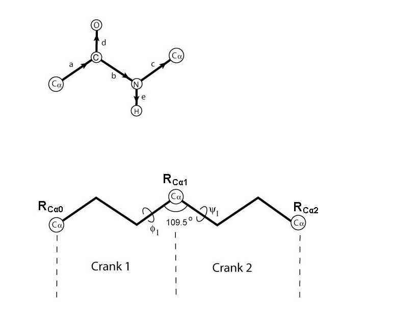
Figure 1: Upper panel shows the “crank” that connects the center of one residue to the next. The vectors a, b, c, d, e represent chemical bonds, which all lie in the same plane. (Side chains have been omitted for clarity). Lower panel shows how the cranks are connected to form the backbone of the protein. The vector position of a C_α is denoted by R_Cαi. The angle between cranks being fixed, the relative orientation of successive cranks is specified by two torsional angles $\phi$ and $\psi$. The conformation of the backbone chain is completely specified by a set of torsional angles. Data for bond lengths and angles are given in Table 1.

Table 1: Bond lengths and bond angles. Data obtained from Protein Data Bank web site (http://www.pdb.org)[4].

	Bond Length (Å)		Bond Angle $(^{\circ})$
Cα-C	1.525	$\angle$CαCN	116.2
C-N	1.329	$\angle$CNCα	121.7
N-Cα	1.458	$\angle$NCαC	109.5
C-O	1.231	$\angle$CαCO	120.8
N-H	1.000	$\angle$CαNH	114.0

The backbone of the protein chain is thus a sequence of cranks. The angle between two adjacent cranks is fixed at the tetrahedral angle $\cos^{-1}(-1/3)\approx 109.5^{\circ}.$ Thus, the orientation of one crank with respect to its predecessor is specified by two torsional angles {$\phi,\psi\},$ as illustrated in Fig. 1.

The conformation of the backbone of the protein is completely specified by a set of torsional angles $\{\phi_{1},\psi_{1};\phi_{2},\psi_{2};\cdots\}.$ In this study, we only consider these torsional degrees of freedom, ignoring the small high-frequency vibrations within the cranks. Such a description has been used in the CSAW model (conditioned self-avoiding walk) of protein folding. [1, 2]

3 Canonical formalism

Consider a chain of $n$ cranks. Let

$$\mathbf{R}_{si} = \text{ position vector of atom }s\text{ on crank }i$$

$$i = 1,\ldots,n$$

$$s = \text{ C}_{\alpha}\text{, C, N, O, H}$$ (1)

We also write this as $\mathbf{R}_{i}$, an array of the position vectors of elements labelled by $s$.

In this study we do not take the side chains into account, so the closest real protein to our model is polyglycine. Formally, it is straightforward to generalize the model.

Let the set of torsional angles be $\{\phi_{i},\psi_{i}\}(i=1,\ldots,n-1).$ Assuming the cranks to be perfectly rigid places constraints on the vector positions. The constraints are solved by using the torsional angles as generalized coordinates, which we denote by the notation

$$q_{ik}\text{ \ }\left(i=1,\ldots,n-1;\text{ }k=1,2\right).$$ (2)

Thus, for example,

$$q_{11}=\phi_{1} q_{12}=\psi_{1}$$

$$q_{21}=\phi_{2} q_{22}=\psi_{2}\text{\ \ \ \ etc.}$$ (3)

We also use the notation $q_{\alpha}$, where $\alpha=\{i,k\}.$ We are to regard $\mathbf{R}_{i}$ as functions of $\{q_{\alpha}\}$.

The velocity is given by

$$\mathbf{\dot{R}}_{i}=\sum_{i=1}^{n-1}\sum_{k=1}^{2}\frac{\partial\mathbf{R}_{i}}{\partial q_{ik}}\dot{q}_{ik}=\sum_{\alpha}\frac{\partial\mathbf{R}_{i}}{\partial q_{\alpha}}\dot{q}_{\alpha}.$$ (4)

The total kinetic energy is

$$K\left(q,\dot{q}\right)=\frac{1}{2}\sum_{i=1}^{n-1}m\mathbf{\dot{R}}_{i}^{2}=\frac{1}{2}\sum_{\alpha,\beta}\dot{q}_{\alpha}\left(\sum_{i=1}^{n-1}m\frac{\partial\mathbf{R}_{i}}{\partial q_{\alpha}}\cdot\frac{\partial\mathbf{R}_{i}}{\partial q_{\beta}}\right)\dot{q}_{\beta}=\frac{1}{2}\dot{q}^{T}M\dot{q}.$$ (5)

where the mass matrix is given by:

$$M_{\alpha\beta}=\sum_{i=1}^{n-1}m\frac{\partial\mathbf{R}_{i}}{\partial q_{\alpha}}\cdot\frac{\partial\mathbf{R}_{i}}{\partial q_{\beta}}.$$ (6)

This is a symmetric matrix, with $M^{T}=M$. We use the shorthand

$$m\mathbf{\dot{R}}_{i}^{2}=\sum\limits_{s}m_{s}\mathbf{\dot{R}}_{si}^{2}.$$ (7)

where $m_{s}$ denotes the mass of atom $s$ on the crank.

The Lagrangian of the backbone chain is given by

$$L(q,\dot{q}) = K(\dot{q},q)-U(q)$$ (8)

$$= \frac{1}{2}\dot{q}^{T}M\dot{q}-U(q).$$

Hence, the canonical momentum is

$$p=\frac{\partial L}{\partial\dot{q}}=M\dot{q}.$$ (9)

and the generalized force is

$$\frac{\partial L}{\partial q}=\frac{1}{2}\dot{q}^{T}\frac{\partial M}{\partial q}\dot{q}-\frac{\partial U}{\partial q}.$$ (10)

The Lagrange equation of motion

$$\frac{d}{dt}\left(\frac{\partial L}{\partial\dot{q}}\right)=\frac{\partial L}{\partial q}$$ (11)

leads to

$$M\ddot{q}=-\frac{1}{2}\dot{q}^{T}\frac{\partial M}{\partial q}\dot{q}-\frac{\partial U}{\partial q}.$$ (12)

The Hamiltonian is

$$H(p,q) = K(p,q)+U(q)$$ (13)

$$= \frac{1}{2}\dot{q}^{T}M\dot{q}+U(q).$$

From (9) we have $\dot{q}=M^{-1}p$ and $\dot{q}^{T}=p^{T}(M^{-1})^{T}$. Therefore,

$$H(p,q)=\frac{1}{2}p^{T}M^{-1}p+U(q).$$ (14)

The canonical equations of motion

$$\dot{p}=-\frac{\partial H}{\partial q},\text{\ }\dot{q}=\frac{\partial H}{\partial p}$$ (15)

take the forms

$$\dot{p} = -\frac{1}{2}p^{T}\frac{\partial M^{-1}}{\partial q}p-\frac{\partial U}{\partial q},$$

$$\dot{q} = M^{-1}p.$$ (16)

These are, of course, the same as the Lagrangian equation of motion (12).

4 The effective potential

The partition function of the system is, up to a constant scale factor, given by

$$Z=\int dq\int dp\ e^{-\beta K(p,q)}e^{-\beta U(q)},$$ (17)

where $\beta=\left(k_{B}T\right)^{-1}$ is the inverse temperature. The $p$-integration is Gaussian, and can be immediately carried out, and the result generally depends on $q$. This gives rise to an effective potential $V_{\text{eff}}(q),$ which is defined through the relation

$$e^{-\beta V_{\text{eff}}(q)}\equiv\left(\frac{\beta}{2\pi}\right)^{n-1}\int dp\ e^{-\beta K(p,q)}.$$ (18)

Thus

$$Z = \int dq\ \rho_{\text{con}}(q),$$

$$\rho_{\text{con}}(q) \equiv e^{-\beta\left(U+V_{\text{eff}}\right)},$$ (19)

where $\rho_{\text{con}}$ is the configurational probability density. That is, $\rho_{\text{con}}dq$ is the relative probability of finding the system in $dq,$ regardless of momentum $p$. If the kinetic energy is independent of $q$, the effective potential is a constant.

In a canonical ensemble, the relative probability of finding the state in element $dpdq$ in phase space is given by $dpdq\exp\left(-\beta H\right)$. If we are only interested in the probability of finding the state in $dq$, we integrate the above over $p$, and obtain

$$dq\int dp\exp\left(-\beta H\right) = dq\exp\left(-\beta U\right)\int dp\exp\left(-\beta K\right)$$ (20)

$$= dq\left(\frac{2\pi}{\beta}\right)^{n-1}\exp\left(-\beta\left(U+V_{\text{eff}}\right)\right).$$

This is the probability to be used, for example, in the Monte-Carlo algorithm in the CSAW model [1, 2].

We now perform the momentum integration:

$$\int dp\ e^{-\beta K(p,q)}=\int dp_{1}\cdots dp_{2(n-1)}\exp\left(-\frac{\beta}{2}p^{T}M^{-1}p\right)=\left(\frac{2\pi}{\beta}\right)^{n-1}\sqrt{\text{det }M}.$$ (21)

Thus

$$\beta V_{\text{eff}}(q)=-\frac{1}{2}\ln\left(\text{det }M\right)=-\frac{1}{2}\text{Tr}\left(\ln M\right).$$ (22)

Since $V_{\text{eff}}(q)$ depends on all the torsional angles, it is a function of the chain conformation. Our calculations show that it is sensibly constant for almost all different conformations. Representative results are shown in Fig. 2.

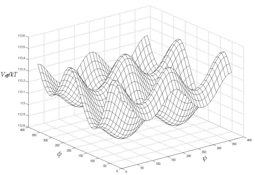
Figure 2: Effective potential of a 3-crank chain at different $\{\phi,\psi\}$ angles between the second and third crank. The percentage change of the effective potential is less than 0.2%.

5 Potential energy of hydrogen bonding

As an application of the canonical formalism, we shall calculate the normal modes of the $\alpha$-helix and the $\beta$-sheet, which are important secondary structures in the folded state of a protein. The main stabilizing agents for these structures are hydrogen bonds, which exist between N-H and C=O groups from different residues [5] [6]. We assume that a hydrogen bond is formed when the distance between the H and O atoms is $2.0\pm 1.0$ Å, and the bond angle between N-H and C=O is $180\pm 45^{\circ}$[5].

The $\alpha$-helix, also known as the 4₁₃-helix, is the most abundant secondary structure due to its tight conformation [6]. In this configuration, a hydrogen bond connects the C=O group of $i$th crank to the N-H group of ($i+3$)th crank.

The $\beta$-sheet is a two-dimensional mat made up of backbone strands stitched together by hydrogen bonds [6].The participating strands may be parallel or antiparallel.

We wish to study the normal modes of small vibrations about an equilibrium configuration. The potential energy $U$ is assumed to be minimum, and taken to be zero, at this configuration. The equilibrium is assumed to be maintained by hydrogen bonds. Deviations from equilibrium arise from the stretching and bending of these bonds. Let $\mathbf{b}_{i}$ be the bond vector of the $i$th hydrogen bond, i.e. the vector between the O and the bonded H, in the equilibrium situation. Let $\mathbf{b}_{i}^{\prime}$ be the same vector when the configuration is displaced from equilibrium. The displacement vector is given by

$$\mathbf{u}_{i}=\mathbf{b}_{i}^{\prime}-\mathbf{b}_{i}.$$ (23)

For small displacements, we take the potential energy to be

$$U=\frac{1}{2}\kappa_{1}\sum_{i}(|\mathbf{\hat{b}}_{i}\cdot\mathbf{u}_{i}|)^{2}+\frac{1}{2}\kappa_{2}\sum_{i}(|\mathbf{\hat{b}}_{i}\times\mathbf{u}_{i}|)^{2}$$ (24)

where $\mathbf{\hat{b}}_{i}=$ $\mathbf{b}_{i}/|\mathbf{b}_{i}|$, and $\kappa_{1}$ and $\kappa_{2}$ are the force constants associated with the stretching and bending of hydrogen bonds, respectively [7]

$$\kappa_{1} = 13\text{ N/m },$$

$$\kappa_{2} = 3\text{ N/m }.$$ (25)

Let the generalized coordinates be denoted

$$q=q_{0}+\lambda$$ (26)

where $q_{0}$ corresponds to equilibrium, and $\lambda$ represents a small deviation. We can write

$$\mathbf{u}_{i}=\sum_{\alpha}\left(\frac{\partial\mathbf{b}_{i}^{\prime}}{\partial q_{\alpha}}\right)_{0}\lambda_{\alpha}+O(\lambda^{2})$$ (27)

where the subscript $0$ indicates evaluation at equilibrium. This leads to the quadratic form

$$U = \frac{1}{2}\lambda^{T}(\kappa_{1}D+\kappa_{2}C)\lambda\ ,$$ (28)

$$D_{\alpha\beta} = \sum_{i}\left|\mathbf{\hat{b}}_{i}\cdot\frac{\partial\mathbf{b}_{i}^{\prime}}{\partial q_{\alpha}}\right|_{0}\cdot\left|\mathbf{\hat{b}}_{i}\cdot\frac{\partial\mathbf{b}_{i}^{\prime}}{\partial q_{\beta}}\right|_{0},$$ (29)

$$C_{\alpha\beta} = \sum_{i}\left|\mathbf{\hat{b}}_{i}\times\frac{\partial\mathbf{b}_{i}^{\prime}}{\partial q_{\alpha}}\right|_{0}\cdot\left|\mathbf{\hat{b}}_{i}\times\frac{\partial\mathbf{b}_{i}^{\prime}}{\partial q_{\beta}}\right|_{0}.$$ (30)

6 Normal Modes

For small oscillations about equilibrium, the linearized equation of motion is

$$M\ddot{\lambda}=-\frac{\partial U}{\partial q}\ .$$ (31)

From (28) we have

$$\frac{\partial U}{\partial q}=(\kappa_{1}D+\kappa_{2}C)\lambda\ .$$ (32)

Thus

$$M\ddot{\lambda}+(\kappa_{1}D+\kappa_{2}C)\lambda=0.$$ (33)

The normal frequencies $\omega$ and normal modes $\lambda$ are eigenvalues and eigenvectors of the equation

$$M^{-1}(\kappa_{1}D+\kappa_{2}C)\lambda=\omega^{2}\lambda\ .$$ (34)

Our model’s validity is subject to the following conditions:

1. We treat small oscillation about a presumed equilibrium configuration $q_{0}$. Whether $q_{0}$ indeed corresponds to equilibrium can be verified through the requirement that all normal frequencies be nonzero and positive.

2. We ignore electrostatic and other interactions. Our results can serve as a test whether the structures investigated can maintain equilibrium purely through hydrogen bonding. Inclusion of other interactions will introduce corrections.

3. Actual $\alpha$ and $\beta$ structures are embedded inside a protein molecule in solution, and are subject to other forces not considered here, particularly those arising from Brownian motion in the solution, the hydrophobic effect, and interaction with other atoms in the protein. These forces will give rise to corrections, and may even destroy the stability of the structure.

In view of the limitations of the model, we only examine normal modes in a frequency range corresponding to wave numbers $10^{-1}-10^{3}$ cm^-1. This is because, in a real protein, the very low-frequency end will be dominated by binding effects to the rest of the protein, while the very high-frequency region will be dominated by bond oscillations.

7 The $\alpha$-helix

We have modelled a generic $\alpha$-helix using torsional angles $\phi,\psi$ from polyalanine [9]

$$\{\phi,\psi\}=\{-57.4^{\circ},\text{ }-47.5^{\circ}\}.$$ (35)

The equivalent spring system is illustrated in Fig. 3. In this example, there are 7 cranks, but only 4 hydrogen bonds. In general, for $n$ cranks, the number of hydrogen bonds is $n-3.$ The number of degrees of freedom from stretching and bending of the hydrogen bonds is thus $2(n-3).$ The total number of degrees of freedom of the system, however, is $2\left(n-1\right).$ Thus we expect to have 4 zero modes, apart from rigid translations and rotations. These will not be included in our results.

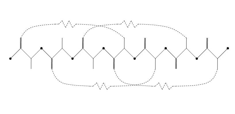
Figure 3: The mechanical system corresponding to small oscillations of the $\alpha$-helix (solid lines). Springs are hydrogen bonds (dashed lines).

Fig. 4 shows the distributions of normal modes as function of wave number, for different crank numbers $n$. All calculated frequencies are positive. The upper panel shows distributions for $n=10-50,$ while the lower panel shows those for $n=60-100.$ In the latter case, the distributions fit a scaling law

$$\text{Density of modes}\varpropto n^{1.3}.$$ (36)

The plotted distributions have been divided by this factor.

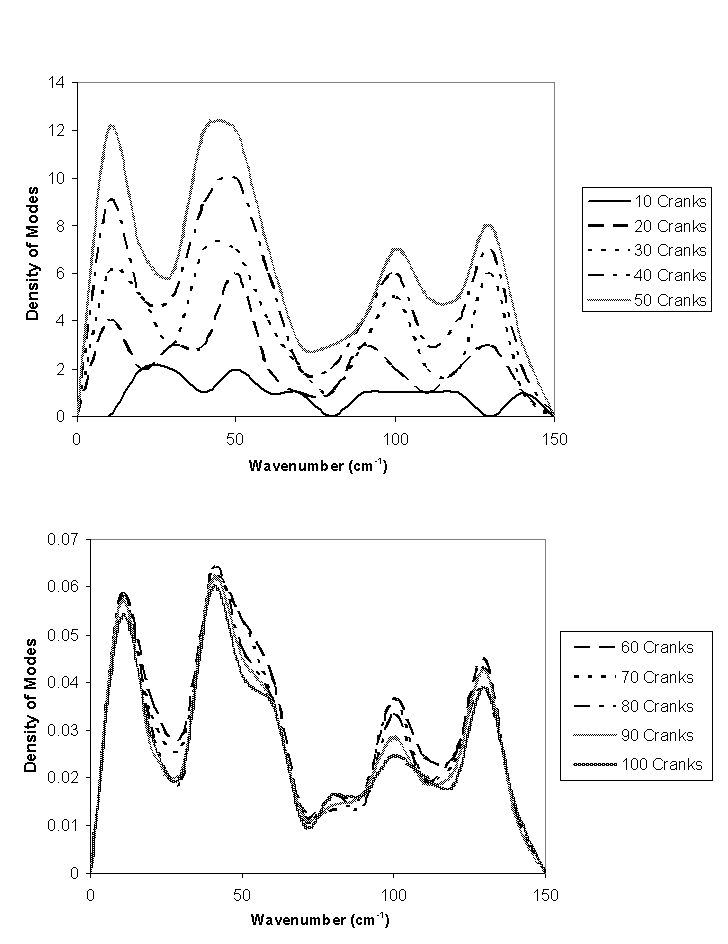
Figure 4: Normal-frequency distributions for the $\alpha$-helix, with different numbers of cranks $n$. Upper panel displays cases $n=10-50.$ Lower panel displays cases $n=60-100$, and the distributions are divided by a scaling factor $n^{1.3}$. Types of distortion corresponding to the peaks are listed in Table 2.

Table 2: Normal modes of $\alpha$-helix.

Frequency (cm-1)	Mode
$0-10$	twisting
$30-40$	stretching & bending
$90-100$	bending
$120-130$	bending

The distributions exhibit 4 peaks associated with various types of deformation, which can be ascertained by examining the corresponding eigenvectors. The results are listed in Table 2.

As an application of our results, we calculate the normal-mode distribution for myoglobin (1MBD) [8], which is made up of 8 alpha-helices, by superposing our calculated distributions. This procedure ignores the interactions between helices, and contributions from the loops connecting the helices, and can only give the crudest approximation to the actual distribution. The result is shown in the upper panel of Fig. 5. The lower panel shows a histogram obtained previously by Krimm and Reisdorf [9], using a different method. There is qualitative agreement, but the peaks are shifted, presumably due to interactions neglected in our simple superposition. The rough shape of the distribution bears resemblance to that calculated for BPTI, a globular protein with 58 residues [10].

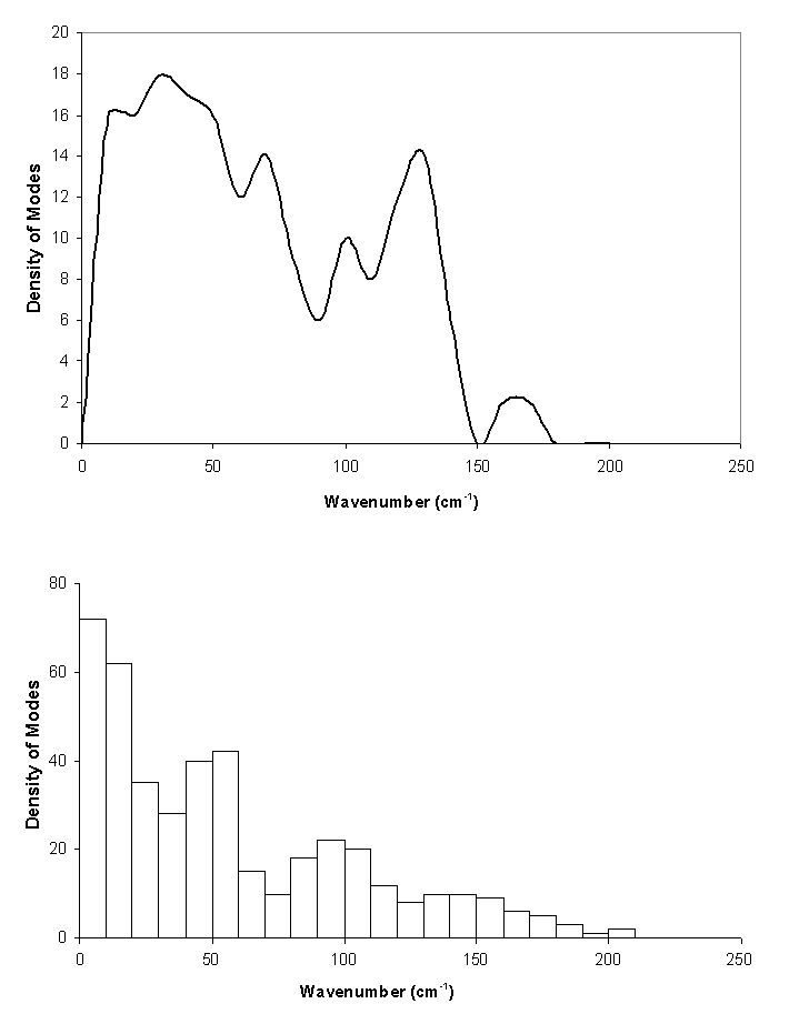
Figure 5: Upper panel: Normal-frequency distribution for myoglobin, constructed by superimposing those of the 8 $\alpha$-helices in the protein. Lower panel:  Result of an independent calculation by Krimm and Reisdorf [9]. There is qualitative agreement, but the peaks are shifted, possibly due to our neglect of interactions between helices, and contributions from loops.

8 The $\beta$-sheet

We model a generic $\beta$-sheet by setting the torsional angles in each strand to

$$\{\phi,\psi\} = \{-139^{\circ},\text{ }135^{\circ}\}\text{ \ \ (antiparallel case \cite[cite]{[\@@bibref{}{MooreKrimm}{}{}]})},$$

$$\{\phi,\psi\} = \{-119^{\circ},\text{ }114^{\circ}\}\text{ \ \ (parallel case \cite[cite]{[\@@bibref{}{BandekarKrimm}{}{}]})}.$$ (37)

The connectivity of hydrogen bonds for the parallel and antiparallel cases is shown in Fig. 6. In the antiparallel case, an extra crank is included to join two adjacent strands. In the parallel case, the strands are left open-ended.

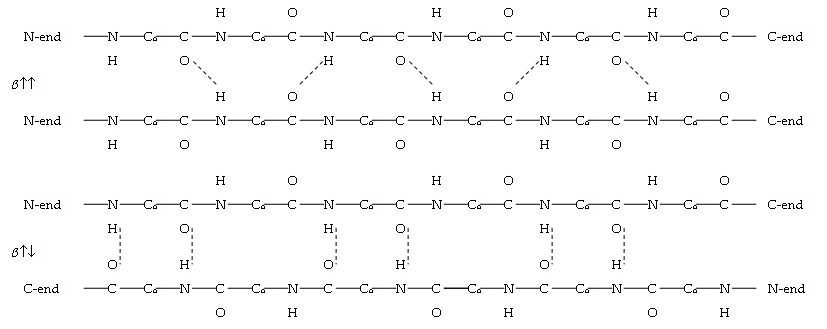
Figure 6: Schematic diagram of $\beta$-sheets, illustrating the connectivity of hydrogen bonds. Upper diagram: parallel $\beta$-sheet. Lower diagram: antiparallel $\beta$-sheet.

Compared to the $\alpha$-helix, the $\beta$-sheet has fewer hydrogen bonds formed within the structure. Thus we expect that in our model there will be more zero modes compared to the $\alpha$-helix; but we ignore them for reasons stated previously. Otherwise, all calculated frequencies are positive.

Normal frequencies are computed for varying numbers of strands, and cranks per strand. We display representative distributions in Fig. 7 for antiparallel and parallel sheets. We see that the frequencies are concentrated around 50 $cm^{-1}$. This is consistent with calculations on real protein with $\beta$-sheet structure [11, 13, 14]. In general, the peak positions of the distributions depend only on the number of cranks per strand, and are independent of the number of strands. The peaks tend to widen with increasing crank number.

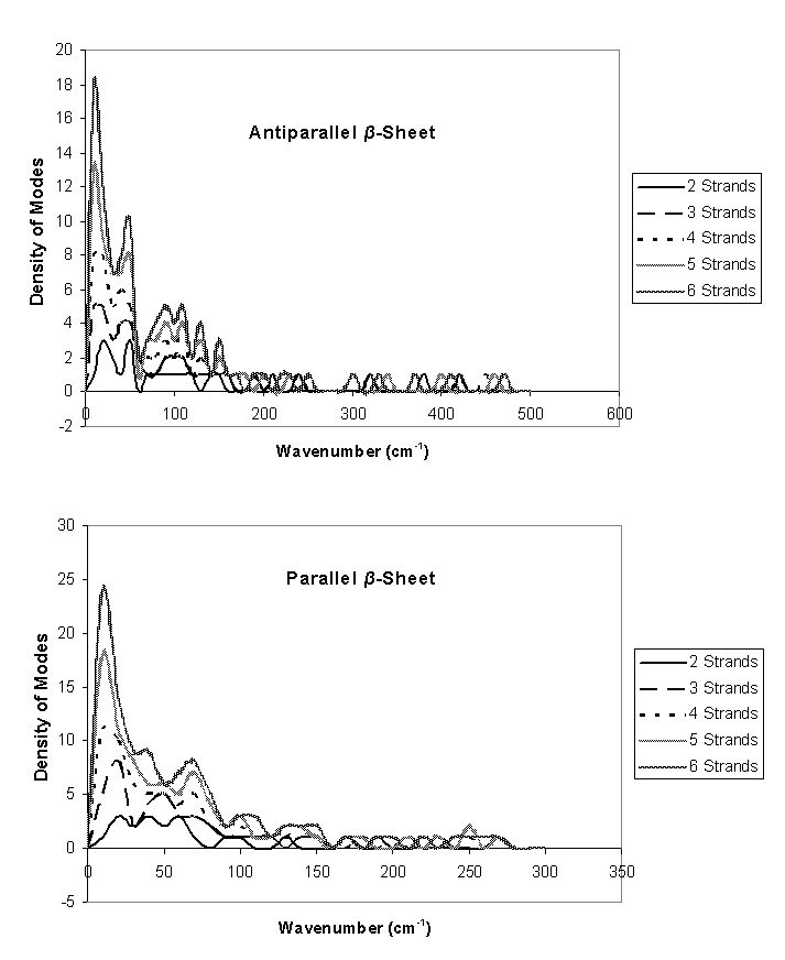
Figure 7: Normal-frequency distributions of $\beta$-sheets, for the same number of cranks per strand, but different number of strands.

9 $\alpha$-$\beta$ transition

The transition between $\alpha$-helix and $\beta$-sheet is an important subject, in view of its possible relevance to the prion transition [3], and the existence of proteins with ambivalent structures [15]. From our results, we can make a crude calculation, which should be taken to be of intuitive, rather than practical value.

We can obtain the free energy of a structure in the neighborhood of equilibrium, by adding the contributions from all of its normal modes, each treated as a harmonic oscillator. For one classical harmonic oscillator of natural frequency $\omega,$ at absolute temperature $T$, the Helmholtz free energy is

$$A_{1}=-k_{B}T\ln\left(\frac{k_{B}T}{\hbar\omega}\right).$$ (38)

For $N$ oscillators, corresponding to $N$ normal modes of frequencies $\omega_{1},\ldots,\omega_{N}$, the total free energy is

$$A_{N} = -Nk_{B}T\ln\left(\frac{k_{B}T}{\hbar\tilde{\omega}}\right);$$

$$\tilde{\omega} = \left(\omega_{1}\cdots\omega_{N}\right)^{1/N}.$$ (39)

Fig. 8 shows the free energies as a function of temperature, for an $\alpha$-helix and an antiparallel $\beta$-sheet, each having 39 cranks. The $\beta$-sheet is made up of 5 strands with 7 cranks per strand.

The expressions for the free energy are valid only when the system is harmonic. As models for secondary structures in a real protein, our results are expected to be valid only in a certain neighborhood of $k_{B}T/\hbar\tilde{\omega}=1$.  How large the neighborhood is depends on interactions between the secondary structure and its environment. Taking these curves on face value, we see from Fig. 8 that they intersect at $T_{c}=20$ $K$, above which the $\alpha$-helix has a lower free energy. In this hypothetical system, then, a transition from $\alpha$-helix to $\beta$-sheet should occur at $T_{c}$, when the temperature is lowered.

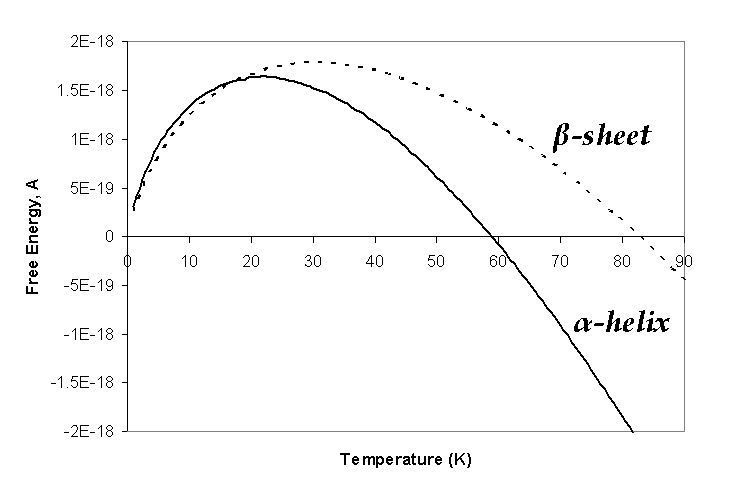
Figure 8: Helmholtz free energy of $\alpha$-helix and $\beta$-sheet, treated as harmonic oscillators with the corresponding normal frequencies. The intersection of the two curves indicates a phase transition. The equilibrium phase is the one with lower free energy.

References

- [1] K. Huang, Biophys. Rev. and Lett. 3, 1 (2008).
- [2] K. Huang, arXiv: cond-mat/0601244 (2006).
- [3] S.B. Prusiner, Proc. Natl. Acad. Sci. USA, 98, 13363 (1998).
- [4] H. M. Berman, J. Westbrook, Z. Feng, G. Gilliland, T. N. Bhat, H. Weissig, I. N. Shindyalov and P. E. Bourne, Nucleic Acids Research, 28, 235 (2002); http://www.pdb.org.
- [5] A. Karshiko, Non-Covalent Interactions in Proteins, (Imperial College Press, London, 2006).
- [6] A.V. Finkelstein and O.B. Ptitsyn, Protein Physics: A Course of Lectures, (Academic Press, London, 2002).
- [7] K. Itoh and T. Shimanouchi, Biopolymers, 9, 383 (1970).
- [8] PDB ID: 1MBD. S. E. Phillips and B.P. Schoenborn, Nature, 292, 81 (1981).
- [9] K. Krimm and W.C. Reisdorf Jr, Faraday Discussions, 99, 181 (1994).
- [10] N. Go, T. Noguchi, T. Nishikawa, Proc. Natl. Acad. Sci. USA, 80, 3696 (1983).
- [11] W.H. Moore and S. Krimm, Biopolymers, 15, 2465 (1976).
- [12] J. Bandekar and S. Krimm, Biopolymers, 27, 909 (1988).
- [13] Y. Abe and S. Krimm, Biopolymers, 11, 1817 (1972).
- [14] A. M. Dwivedi and S. Krimm, Macromolecules, 15, 186 (1982).
- [15] S. Patel, P.V. Baleji, and Y.U. Sasidhar, J. Peptide Sci., 13, 314 (2007).