Smart detectors for Monte Carlo radiative transfer

Abstract

Many optimization techniques have been invented to reduce the noise that is inherent in Monte Carlo radiative transfer simulations. As the typical detectors used in Monte Carlo simulations do not take into account all the information contained in the impacting photon packages, there is still room to optimize this detection process and the corresponding estimate of the surface brightness distributions. We want to investigate how all the information contained in the distribution of impacting photon packages can be optimally used to decrease the noise in the surface brightness distributions and hence to increase the efficiency of Monte Carlo radiative transfer simulations.

We demonstrate that the estimate of the surface brightness distribution in a Monte Carlo radiative transfer simulation is similar to the estimate of the density distribution in an SPH simulation. Based on this similarity, a recipe is constructed for smart detectors that take full advantage of the exact location of the impact of the photon packages. Several types of smart detectors, each corresponding to a different smoothing kernel, are presented. We show that smart detectors, while preserving the same effective resolution, reduce the noise in the surface brightness distributions compared to the classical detectors. The most efficient smart detector realizes a noise reduction of about 10%, which corresponds to a reduction of the required number of photon packages (i.e. a reduction of the simulation run time) of 20%. As the practical implementation of the smart detectors is straightforward and the additional computational cost is completely negligible, we recommend the use of smart detectors in Monte Carlo radiative transfer simulations.

1 Introduction

The Monte Carlo method (e.g. Cashwell & Everett, 1959; Bianchi, Ferrara, & Giovanardi, 1996; Gordon et al., 2001; Baes et al., 2003; Niccolini, Woitke, & Lopez, 2003) has become one of the most popular methods to perform radiative transfer simulations. One of the greatest advantages of the Monte Carlo method is its conceptual simplicity. Instead of solving the radiative transfer equations that describe the radiation field, Monte Carlo simulations actually follow the photon packages that make up the radiation field in a very natural way. This ensures that, compared to other approaches to multi-dimensional radiative transfer problems, the practical implementation of Monte Carlo radiative transfer is surprisingly straightforward. This simple, straightforward approach also enables the inclusion of additional ingredients, such as the polarization of scattered light (Code & Whitney, 1995; Bianchi, Ferrara, & Giovanardi, 1996), the kinematics of the sinks and sources (Matthews & Wood, 2001; Baes & Dejonghe, 2002) and gas ionization and recombination processes (Ercolano et al., 2003; Ercolano, Barlow, & Storey, 2005). On the other hand, probably the most important disadvantage of the Monte Carlo method is the appearance of Poisson noise, which is inherently tied to the probabilistic nature of the method. In pure Monte Carlo radiative transfer simulations, the noise in any observed property goes as $1/\sqrt{N}$ with $N$ the number of photon packages, which means that one needs to quadruple the number of photon packages to halve the errors. Due to this slow convergence, radiative transfer simulations based on the most simple application of the Monte Carlo method are very inefficient and have difficulties to compete with other methods.

Fortunately, in the many years since the first applications of the Monte Carlo method to radiative transfer simulations, several intelligent optimization techniques have been invented to increase the efficiency of the Monte Carlo techniques. These techniques, equivalent to so-called variance reduction techniques in Monte Carlo integration, aim at reducing the noise by including deterministic elements into the probabilistic simulation. One of the first examples of such techniques is the well-known forced first scattering technique, already included in the first implementations of Monte Carlo radiative transfer (Cashwell & Everett, 1959; Mattila, 1970). Other noise-reduction techniques that have strongly increased the efficiency of the Monte Carlo method include the use of weighted photon packages (Witt, 1977), the peel-off technique (Yusef-Zadeh, Morris, & White, 1984), the treatment of absorption as a continuous rather than a discrete process (Lucy, 1999), the frequency distribution adjustment technique (Bjorkman & Wood, 2001; Baes et al., 2005) and the use of polychromatic photon packages (Baes, Dejonghe, & Davies, 2005; Jonsson, 2006).

One aspect of Monte Carlo radiative transfer where no significant noise reduction techniques have been presented is the last step in the life cycle of the photon packages, namely their detection. The goal of most Monte Carlo radiative transfer simulations is to determine the observed surface brightness distribution at some observer’s position. To construct the observed surface brightness distribution, some kind of detector must be simulated, on which the photon packages that leave the system are recorded. In the spirit that Monte Carlo radiative transfer simulations mimic the real physical processes as naturally as possible, the simulated detectors are usually natural (idealized) representations of actual CCD detectors. They basically consist of a two-dimensional array of pixels, which act as a reservoir for the incoming photon packages. When a photon package leaves the system and arrives at the location of the observer, the correct bin is determined and the luminosity recorded in the bin is increased with the luminosity of the photon package. At the end of the simulation, the detector is read out like a CCD detector and the surface brightness distribution is constructed.

While this approach seems the most natural way to simulate the detection of photon packages in a Monte Carlo simulation, it might not be the most efficient. We must be aware that, although we are simulating a real detection as closely as possible, we have more information at our disposal than real observers. The maximum information that a real observer can obtain (in the academic limit of perfect noise-free observations and instruments) when imaging with a CCD detector, is the number of photon packages that arrive in each of his pixels. As numerical simulators, we have at our disposal the full information on the precise location of the impact of each photon package on the detector. It would be a pity to throw away this useful additional information just in order to mimic the behaviour of a real CCD detector.

The goal of this paper is to investigate how this additional information can be used to decrease the noise in the estimated surface brightness distributions and hence to increase the efficiency of Monte Carlo radiative transfer simulations. In Section 2 we describe the classical way of detecting photon packages as a smoothing process, similar to the averaging processes encountered in the smoothed particle hydrodynamics framework for hydrodynamical simulations. We use this similarity between both processes to construct a new set of smart detectors, which aim at curing two drawbacks of the classical detectors. In Section 3 we test the accuracy and performance of these smart detectors and compare them with the classical detector. The results are summarized and discussed in Section 4.

2 Smart detectors

2.1 The classical detector

A typical detector in Monte Carlo simulations is based on a realistic CCD detector. It consists of a rectangular two-dimensional array of bins of dimension $\Delta$ placed on the plane of the sky. We denote the centre positions of these bins as $\bar{\boldsymbol{x}}_{ij}=(\bar{x}_{i},\bar{y}_{j})$,

$$\bar{x}_{i}=\bar{x}_{\text{min}}+i\,\Delta,$$ (1)

$$\bar{y}_{j}=\bar{y}_{\text{min}}+j\,\Delta.$$ (2)

When the $k$’th photon package hits the detector at a certain position ${\boldsymbol{x}}_{k}=(x_{k},y_{k})$, we find out in which bin it will end, and we add the luminosity $L_{k}$ carried by photon package to the number of previously detected photon packages in this particular bin. At the end of the simulation, we determine our estimate $I_{\text{s}}(\bar{\boldsymbol{x}}_{ij})$ for the surface brightness at the position $\bar{\boldsymbol{x}}_{ij}$ by summing the contribution of all photon packages that have been recorded in that bin and correcting for the surface of the bin,

$$I_{\text{s}}(\bar{\boldsymbol{x}}_{ij})=\frac{1}{\Delta^{2}}\sum_{k=1}^{N}L_{k}\,N_{ij}({\boldsymbol{x}}_{k})$$ (3)

where

$$N_{ij}({\boldsymbol{x}})=\begin{cases}\;1&\quad\text{if $\bar{x}_{i}-\tfrac{1}{2}\Delta\leq x\leq\bar{x}_{i}+\frac{1}{2}\Delta$}\\ &\qquad\text{and $\bar{y}_{j}-\tfrac{1}{2}\Delta\leq y\leq\bar{y}_{j}+\frac{1}{2}\Delta$},\\[10.00002pt] \;0&\quad\text{else}.\end{cases}$$ (4)

2.2 The link to SPH

For an interesting point of view on simulating the detection of photon packages and the calculation of the surface brightness distribution, we now shift to another important technique in computational astrophysics, namely smoothed particle hydrodynamics or SPH (Gingold & Monaghan, 1977; Lucy, 1977). SPH is a computational technique for hydrodynamical simulations in which the a fluid is represented as a finite collection of fluid elements. To estimate the value of a physical field $f({\boldsymbol{r}})$ at an arbitrary position ${\boldsymbol{r}}$, we must perform local averages over volumes of nonzero extent (i.e. over a finite number of fluid particles). The mean or smoothed value of $f({\boldsymbol{r}})$, denoted as $f_{\text{s}}({\boldsymbol{r}})$ can be determined through kernel estimation,

$$f_{\text{s}}({\boldsymbol{r}})=\iiint W({\boldsymbol{r}}-{\boldsymbol{r}}^{\prime})\,f({\boldsymbol{r}}^{\prime})\,{\text{d}}{\boldsymbol{r}}^{\prime},$$ (5)

where $W({\boldsymbol{r}})$ is the so-called smoothing kernel, which should be normalized according to

$$\iiint W({\boldsymbol{r}})\,{\text{d}}{\boldsymbol{r}}=1,$$ (6)

and which typically is strongly peaked about ${\boldsymbol{r}}=0$. In particular, if the fluid mass distribution $\rho({\boldsymbol{r}})$ is represented by a flow of $N$ particles with mass $m_{k}$, we have

$$\rho({\boldsymbol{r}})=\sum_{k=1}^{N}m_{k}\,\delta({\boldsymbol{r}}-{\boldsymbol{r}}_{k}),$$ (7)

and the estimate $\rho_{\text{s}}({\boldsymbol{r}})$ for the mass distribution is given by

$$\rho_{\text{s}}({\boldsymbol{r}})=\sum_{k=1}^{N}m_{k}\,W({\boldsymbol{r}}-{\boldsymbol{r}}_{k}).$$ (8)

The standard interpretation of this formula is to see the fluid elements that make up the representation of the fluid not as point-like particles, but as particles with a smoothed smeared out mass distribution $\rho_{k}({\boldsymbol{r}})=m_{k}\,W({\boldsymbol{r}}-{\boldsymbol{r}}_{k})$. The total density at any position ${\boldsymbol{r}}$ is then the sum of the contribution of the $N$ particles in the fluid.

Returning back to our simulated CCD detector, we note that we can write expression (3) as

$$I_{\text{s}}(\bar{\boldsymbol{x}}_{ij})=\sum_{k=1}^{N}L_{k}\,W(\bar{\boldsymbol{x}}_{ij}-{\boldsymbol{x}}_{k}),$$ (9)

with $W({\boldsymbol{x}})$ a function defined as

$$W({\boldsymbol{x}})=\left[\frac{H\left(x+\tfrac{1}{2}\Delta\right)-H\left(x-\tfrac{1}{2}\Delta\right)}{\Delta}\right]\,\\ \times\left[\frac{H\left(y+\tfrac{1}{2}\Delta\right)-H\left(y-\tfrac{1}{2}\Delta\right)}{\Delta}\right]\,$$ (10)

with $H$ the Heaviside step function. Comparing equations (9) and (8) we immediately see a connection between the computation of the (three-dimensional) mass density in fluids in the SPH formalism and the computation of the (two-dimensional) surface brightness in a Monte Carlo radiative transfer simulation. We can make this connection clearer by rewriting equation (9) as

$$I_{\text{s}}(\bar{\boldsymbol{x}}_{ij})=\iint W(\bar{\boldsymbol{x}}_{ij}-{\boldsymbol{x}}^{\prime})\,I({\boldsymbol{x}}^{\prime})\,{\text{d}}{\boldsymbol{x}}^{\prime},$$ (11)

with

$$I({\boldsymbol{x}})=\sum_{k=1}^{N}L_{k}\,\delta({\boldsymbol{x}}-{\boldsymbol{x}}_{k}).$$ (12)

Since this latter expression is nothing but the “true” surface brightness distribution corresponding to $N$ photon packages hitting the detector plane (each photon package results in a Dirac delta function), equation (11) is the direct analogue of the SPH basic equation (5). The bottom-line is that we can interpret the radiation field at the plane of the sky as a fluid, which is represented by a finite number of smoothed photon packages. Each smoothed photon package corresponds to a smeared out surface brightness distribution $I_{k}({\boldsymbol{x}})=L_{k}\,W({\boldsymbol{x}}-{\boldsymbol{x}}_{k})$. Formula (9) shows that the total observed surface brightness distribution at the positions ${\boldsymbol{x}}_{ij}$ is the sum of the contributions of each of these photon packages.

2.3 Smart detectors

We have seen that we can interpret the determination of the surface brightness distribution in a Monte Carlo radiative transfer simulation as a smoothing operation similar to the averaging in SPH hydrodynamical simulations. As in SPH simulations, we can consider using a different kernel — in the present case this corresponds to a different kind of detector. In principle, there is no restriction on the shape of the function $W({\boldsymbol{x}})$ apart from the normalization condition

$$\iint W({\boldsymbol{x}})\,{\text{d}}{\boldsymbol{x}}=1,$$ (13)

and the requirement that $W({\boldsymbol{x}})$ is a centrally peaked function. This freedom allows us to construct smart detectors which improve upon a number of potential disadvantages of the traditional detector.

A first drawback of the smoothing kernel (10) is that it is not isotropic, meaning that it has a preferential direction. Not all photon packages hitting the detector at the same given distance from a grid point $\bar{\boldsymbol{x}}_{ij}$ have the same impact on the surface brightness. For example, a photon package hitting the detector at

$${\boldsymbol{x}}_{k}=\left(\bar{x}_{i}+\tfrac{2}{3}\,\Delta,\bar{y}_{j}\right)$$ (14)

will not contribute at all to the surface brightness $I_{\text{s}}({\boldsymbol{x}}_{ij})$, whereas a photon package hitting the detector at

$${\boldsymbol{x}}_{k}=\left(\bar{x}_{i}+\sqrt{\tfrac{2}{3}}\,\Delta,\bar{y}_{j}+\sqrt{\tfrac{2}{3}}\,\Delta\right),$$ (15)

at the same distance, will fully contribute to the estimate of the surface brightness at this grid point. It is obvious that this problem is solved when we consider circularly symmetric smoothing kernels $W({\boldsymbol{x}})\equiv W(R)$.

A second drawback of the classical detector is that it does not take into account all the information that is contained in the impacting photon package. For every photon package that falls onto our detector, we know the exact location of the impact. The only information that a classical simulated detector uses is the bin in which this location falls, without any discrimination of the exact location within this bin. As argued in the introduction, it would be a pity to not use this information just for the sake of simulating a real CCD detector. To solve the second problem, we need to look for kernels that give more weight to impacts very close to the grid points than to impacts at larger distance, which means that we need a kernel $W(R)$ that is a monotonically decreasing function of $R$.

These are just minor limitations and still leave a lot of room for different smart detectors. We can inspire ourselves on the smoothing kernels that are often used in SPH simulations. The prototypical normalized kernel is a gaussian, in two dimensions,

$$W(R)=\frac{1}{\pi h^{2}}\,\exp\left(-\frac{R^{2}}{h^{2}}\right).$$ (16)

The parameter $h$ in this expression, and in all other kernels we will discuss, is called the smoothing length. It gives the width of the area over which the smoothing is effective (we will later determine the optimal value for this parameter). An important drawback of the gaussian kernel is its infinite support, meaning that every photon package impacting on the detector has a finite contribution to the surface brightness at all grid points. Every photon package hence in principle requires a summation over all grid points, at most of which it contributes an absolutely negligible contribution.

These efficiency problems are resolved by introducing smoothing kernels with a compact support. Several compact support kernels have been used in the SPH literature, the most popular of them being kernels based on B-splines. The $M_{3}$ spline kernel (Hockney & Eastwood, 1981) in two dimensions takes the form

$$W(R)=\frac{16}{13\pi h^{2}}\times\begin{cases}\;\frac{3}{2}-2\,u^{2}&\quad\text{if $0\leq u\leq\tfrac{1}{2}$},\\[5.0pt] \;(\tfrac{3}{2}-u)^{2}&\quad\text{if $\tfrac{1}{2}\leq u\leq\tfrac{3}{2}$},\\[5.0pt] \;0&\quad\text{else},\end{cases}$$ (17)

with $u=R/h$. It has a continuous first derivative. A similar spline kernel but with a continuous second derivative is the $M_{4}$ spline smoothing kernel, introduced by Monaghan & Lattanzio (1985). Its two-dimensional form is

$$W(R)=\frac{10}{7\pi h^{2}}\times\begin{cases}\;1-\frac{3}{2}\,u^{2}+\tfrac{3}{4}\,u^{3}&\quad\text{if $0\leq u\leq 1$},\\[5.0pt] \;\tfrac{1}{4}\,(2-u)^{3}&\quad\text{if $1\leq u\leq 2$},\\[5.0pt] \;0&\quad\text{else}.\end{cases}$$ (18)

In principle, we have not requested that the kernel is everywhere non-negative. Some SPH simulations have adopted so-called superkernels, which are accurate to third or fourth order, but which necessarily become negative in some part of the domain. The most famous example of such kernels is the supergaussian kernel (Gingold & Monaghan, 1982) but examples with finite support have also been considered (Monaghan, 1985, 1992; Capuzzo-Dolcetta & Di Lisio, 2000). Using such superkernels could potentially increase the accuracy of the smoothing process, but it can have serious consequences when there is a sharp change in the surface brightness: an undershoot occurs and the recorded surface brightness may become negative. In order to avoid such situations, we stick to positive kernels.

2.4 Determination of the smoothing length

Based on the three smoothing kernels (16), (17) and (18) we can construct three different kinds of smart detectors. Remains to determine which value to take for the smoothing length $h$ for each of these smart detectors. Obviously, $h$ should be large enough to make the smoothing operation meaningful, whereas too large values of $h$ will tend to over-smooth and wash away the details of the surface brightness distribution. We want the smoothing lengths comparable with the pixel scale, such that the noise in the images remains uncorrelated on a pixel-by-pixel scale (as for a classical detector). Our determination of the optimal smoothing length is derived from the requirement that the effective area or “resolution” of the smoothing kernel should be identical to the resolution of the classical detector.

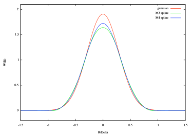
Figure 1: The three smoothing kernels used for the construction of the smart detectors. The normalization and the width is the same for all three kernels.

There are various possibilities to identify the effective area of a two-dimensional centrally peaked function. Probably the most general one is the total dispersion $\sigma$, defined through

$$\sigma^{2}=\iint W({\boldsymbol{x}})\,|{\boldsymbol{x}}|^{2}\,{\text{d}}{\boldsymbol{x}}.$$ (19)

One can readily verify that the classical detector kernel (10) has a dispersion $\sigma=\Delta/\sqrt{6}$. Requiring that the resolution of the other smoothing kernels are equal to this value we find as reference smoothing lengths

$$h_{\text{ref}} =\dfrac{1}{\sqrt{6}}\,\Delta\approx 0.408\,\Delta \text{(gaussian)},$$ (20)

$$h_{\text{ref}} =\dfrac{\sqrt{390}}{33}\,\Delta\approx 0.598\,\Delta \text{($M_{3}$ spline)},$$ (21)

$$h_{\text{ref}} =\dfrac{7}{\sqrt{186}}\,\Delta\approx 0.513\,\Delta \text{($M_{4}$ spline)}.$$ (22)

Figure 1 shows a comparison of the three different smoothing kernels with their optimal smoothing lengths.

3 Tests

3.1 Comparison of classical and smart detectors

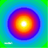
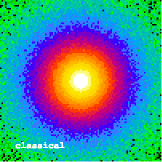
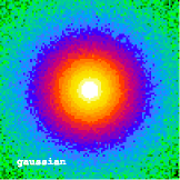
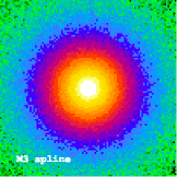
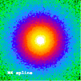
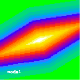
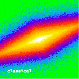
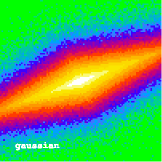
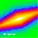
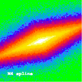
Figure 2: The Plummer (top) and exponential disc (bottom) model surface brightness distribution $I({\boldsymbol{x}}_{ij})$ and the observed surface brightness distributions $I_{\text{s}}({\boldsymbol{x}}_{ij})$ for the classical and the smart detectors. The images have $101\times 101$ pixels each and are based on the simulation with $N=10^{6}$ photon packages.

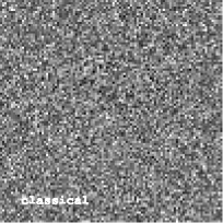
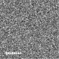
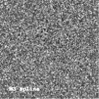
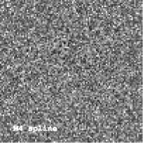
Figure 3: The noise distributions $\Delta I({\boldsymbol{x}}_{ij})$ corresponding to the observed Plummer surface brightness distributions displayed in Figure 2.

We tested the accuracy and the performance of our smart detectors using two toy analytical surface brightness distributions on the plane of the sky. The first is a simple Plummer model, characterized by the circularly symmetric surface brightness distribution

$$I({\boldsymbol{x}})=\frac{L}{\pi b^{2}}\left(\frac{b^{2}}{b^{2}+R^{2}}\right)^{2},$$ (23)

with $L$ the total luminosity and $b$ a scale parameter. We took the value $b=10\Delta$, implying that the core of the model is well resolved by the detector grid. The second model is an exponential disc model, rotated over an angle of 20 degrees,

$$I({\boldsymbol{x}})=\frac{L}{4\pi h_{x}h_{y}}\,\exp\left(-\frac{|x|}{h_{x}}-\frac{|y|}{h_{y}}\right),$$ (24)

with $h_{x}$ and $h_{y}$ the scalelength and scaleheight respectively. Choosing the disc parameters as $h_{x}=25\Delta$ and $h_{y}=5\Delta$, we create a model with a relatively sharp edge and a strong gradient in the surface brightness distribution.

We have used a classical detector and three smart detectors based on the smoothing kernels (16), (17) and (18), each of them with a total of $101\times 101$ grid points. For each model, we ran a set of Monte Carlo simulations with the number of photon packages varying between $N=10^{4}$ and $N=10^{8}$, taking into account that each detector measures the same set of photon packages (i.e. we use the same Monte Carlo realisation for simulations with different detectors).

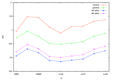
Figure 4: The total noise parameter ${\mathcal{R}}$, defined in equation (26), of the Plummer model for different detectors as a function of the total number of photon packages in the simulation.

The different panels of figure 2 show the resulting measured surface brightness distribution $I_{\text{s}}({\boldsymbol{x}})$ for the various detectors for the simulations with $N=10^{6}$. Looking at this set of images, it is immediately clear that the smart detectors manage to qualitatively reproduce the surface brightness distribution accurately. For a measure of the accuracy of the different detectors, we consider the noise as the difference between the measured surface brightness and the theoretical surface brightness in each pixel, weighted by the expected Poisson noise $\sigma(x_{ij})$ in each pixel,

$$\Delta I({\boldsymbol{x}}_{ij})=\frac{I_{\text{s}}({\boldsymbol{x}}_{ij})-I({\boldsymbol{x}}_{ij})}{\sigma({\boldsymbol{x}}_{ij})}.$$ (25)

Figure 3 show the noise images corresponding to the Plummer model images from Figure 2. It is clear that these images are qualitatively very similar; thanks to the appropriate choice of the smoothing lengths for the different kernels, there is no correlation in the noise on a pixel-by-pixel scale. A quantitative analysis of these noise images, however, shows that the level of the noise in the smart detectors is suppressed. This is most easily demonstrated using the total noise level, which we define as

$${\mathcal{R}}=\frac{\sqrt{N}}{N_{\text{pix}}}\sum\left[\frac{I_{\text{s}}({\boldsymbol{x}}_{ij})-I({\boldsymbol{x}}_{ij})}{\sigma({\boldsymbol{x}}_{ij})}\right]^{2},$$ (26)

where the sum runs over all pixels. A factor $\sqrt{N}$ is included in this formula to guarantee that the noise is asymptotically independent of the total number $N$ of photon packages used in the simulation. Figure 4 shows the value of ${\mathcal{R}}$ for the different detectors as a function of the total number of photon packages in the simulation. This figure demonstrates that all smart detectors reduce the noise compared to the classical detector. The most efficient detector is the one based on the $M_{3}$ spline kernel; for this detector the noise is reduced by about 10%. For the $M_{4}$ spline kernel, the most popular finite support kernel in SPH simulations, the noise reduction is slightly less efficient (about 8%), whereas for the gaussian kernel the noise reduction is about 5%.

3.2 Origin of the noise reduction

We have constructed our smart detectors based on two fundamental changes applied to the classical detector smoothing kernel (10), namely making it circularly symmetric and choosing a smoothly decreasing function of radius. We can investigate which of these two changes has the most important impact on the noise reduction by constructing two new smoothing kernels in which only one of these two changes is taken into account.

On the one hand, the circularly symmetric analogue of the classical detector kernel (10) is readily found,

$$W(R)=\frac{4}{\pi h^{2}}\,\left[H\left(R+\tfrac{1}{2}h\right)-H\left(R-\tfrac{1}{2}h\right)\right].$$ (27)

We find in the usual way $h_{\text{ref}}=2\Delta/\sqrt{3}$ as reference smoothing length. On the other hand, the rectangular version of the $M_{3}$ spline kernel (17) is

$$W({\boldsymbol{x}})=\frac{1}{h^{2}}\,M_{3}\left(\frac{|x|}{h}\right)\,M_{3}\left(\frac{|y|}{h}\right),$$ (28)

with

$$M_{3}(u)=\begin{cases}\;\frac{3}{4}-u^{2}&\quad\text{if $0\leq u\leq\tfrac{1}{2}$},\\[5.0pt] \;\tfrac{1}{2}\,(\tfrac{3}{2}-u)^{2}&\quad\text{if $\tfrac{1}{2}\leq u\leq\tfrac{3}{2}$},\\[5.0pt] \;0&\quad\text{else}.\end{cases}$$ (29)

For this kernel we obtain $h_{\text{ref}}=\Delta/\sqrt{3}$.

In Figure 5 we plot the total noise parameter ${\mathcal{R}}$ of these two new smart detectors in comparison with the classical detector and the circularly symmetric $M_{3}$ spline detector. Not surprisingly, we find that also these two new detectors suppress the noise compared to the classical detector, but not as efficiently as the $M_{3}$ spline detector. The noise reduction in a detector based on the rectangular $M_{3}$ spline kernel (28) is more effective than the noise reduction in the circular analogue (27) of the classical detector. This means that applying a proper weight to the photon packages according to their distance from the grid points is the most important change if we want efficient noise reduction.

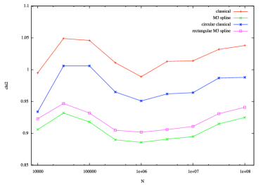
Figure 5: The total noise parameter ${\mathcal{R}}$ of the Plummer model for the rectangular and circular equivalents of the classical detector and the smart $M_{3}$ spline detector.

4 Discussion and conclusions

We have focused on an ill-studied area of Monte Carlo radiative transfer simulations where a significant noise reduction can be achieved, namely the detection of photon packages and the corresponding construction of the observed surface brightness distribution. The motivation of this work was the fact that the classical detectors used in Monte Carlo simulations, while closely mimicking a real CCD detector, do not use the full amount of information that is available.

Based on the similarities between the construction of the surface brightness distribution on a detector in Monte Carlo radiative transfer simulations and the calculation of the density in SPH hydrodynamical simulations, we have constructed a set of smart detectors. These smart detectors improve on two aspects of the classical detector: they assign the same weight to all photon packages hitting the detector at the same distance from a grid point and they give more weight to impacts close to a grid point than to impacts at larger distances. We have tested different kinds of smart detectors, based on different smoothing kernels frequently encountered in SPH simulations, namely a gaussian kernel and two spline-based kernels with finite support (Hockney & Eastwood, 1981; Monaghan & Lattanzio, 1985). We have shown that these new detectors, while preserving the same effective resolution, reduce the noise in the surface brightness distributions compared to the classical detectors. It is demonstrated that the lion’s share of this noise reduction is due to a proper weighing of the photon packages with the distance between the impact location and the grid point.

The most efficient smart detector is found to be a detector based on the $M_{3}$ spline kernel, for which the noise reduction amounts to some 10%. While this might seem a modest improvement, one should take into account that the noise reduction in Monte Carlo simulation goes as $1/\sqrt{N}$. A reduction of the noise with 10% is hence equivalent to a reduction of the number of photon packages with 20%, which is a significant improvement. Moreover, it should be stressed that this noise reduction basically comes for free, since the practical implementation of the smart detectors is straightforward and the additional computational cost is completely negligible. We hence strongly recommend the use of smart detectors in Monte Carlo radiative transfer simulations.

The link with SPH simulations might stimulate to look for further ways to optimize the estimates of the surface brightness distribution. One major difference between our current problem and the interpolation in SPH simulations is that we use a fixed smoothing length, whereas SPH simulations typically use a spatially (and temporally) varying smoothing length. This way it is possible to take full advantage of the particle distribution to resolve local density structures. Each particle in an SPH simulation typically has an individual smoothing length which is fine-tuned such that each particle interacts with a similar number of neighbors. Unfortunately, it seems hard to introduce variable smoothing lengths here in our current Monte Carlo radiative transfer case. The main difference is that the smoothing procedure in SPH is executed when all particle positions are known, whereas in Monte Carlo radiative transfer the photon packages gradually hit the detector and they must be smoothed out onto the detector before it is known where the other photon packages will arrive. It is impossible to know a priori how many neighbors a photon package will ultimately have and hence to adapt the smoothing length on an individual basis. One could potentially do a test run with a limited number of photon packages to obtain a first crude estimate of the expected surface brightness distribution and adapt the smoothing lengths accordingly. However, a more elegant option seems to apply an adaptive filtering to the simulated images after the simulation. Several approaches have been developed for this goal such as wavelet-based algorithms (Starck & Pierre, 1998), adaptive binning techniques (Starck & Pierre, 1998; Cappellari & Copin, 2003) or adaptive kernel smoothing techniques (Richter et al., 1991; Huang & Sarazin, 1996; Ebeling, White, & Rangarajan, 2006).

References

- Baes & Dejonghe (2002) Baes M., Dejonghe H., 2002, MNRAS, 335, 441
- Baes, Dejonghe, & Davies (2005) Baes M., Dejonghe H., Davies J. I., 2005, AIPC, 761, 27
- Baes et al. (2003) Baes M., et al., 2003, MNRAS, 343, 1081
- Baes et al. (2005) Baes M., Stamatellos D., Davies J. I., Whitworth A. P., Sabatini S., Roberts S., Linder S. M., Evans R., 2005, NewA, 10, 523
- Bianchi, Ferrara, & Giovanardi (1996) Bianchi S., Ferrara A., Giovanardi C., 1996, ApJ, 465, 127
- Bjorkman & Wood (2001) Bjorkman J. E., Wood K., 2001, ApJ, 554, 615
- Cappellari & Copin (2003) Cappellari M., Copin Y., 2003, MNRAS, 342, 345
- Capuzzo-Dolcetta & Di Lisio (2000) Capuzzo-Dolcetta R., Di Lisio R., 2000, Applied Numerical Mathematics, 34, 363
- Cashwell & Everett (1959) Cashwell E. D., Everett C. J., 1959, A Practical Manual on the Monte Carlo Method for Random Walk Problems, Pergamom Press
- Code & Whitney (1995) Code A. D., Whitney B. A., 1995, ApJ, 441, 400
- Ebeling, White, & Rangarajan (2006) Ebeling H., White D. A., Rangarajan F. V. N., 2006, MNRAS, 368, 65
- Ercolano et al. (2003) Ercolano B., Barlow M. J., Storey P. J., Liu X.-W., 2003, MNRAS, 340, 1136
- Ercolano, Barlow, & Storey (2005) Ercolano B., Barlow M. J., Storey P. J., 2005, MNRAS, 362, 1038
- Gingold & Monaghan (1977) Gingold R. A., Monaghan J. J., 1977, MNRAS, 181, 375
- Gingold & Monaghan (1982) Gingold R. A., Monaghan J. J., 1977, J. Comp. Phys., 149, 135
- Gordon et al. (2001) Gordon K. D., Misselt K. A., Witt A. N., Clayton G. C., 2001, ApJ, 551, 269
- Hockney & Eastwood (1981) Hockney R. W., Eastwood J. W., 1981, Computer Simulations Using Particles, New York: McGraw-Hill
- Huang & Sarazin (1996) Huang Z., Sarazin C. L., 1996, ApJ, 461, 622
- Jonsson (2006) Jonsson P., 2006, MNRAS, 372, 2
- Lorenz et al. (1993) Lorenz H., Richter G. M., Capaccioli M., Longo G., 1993, A&A, 277, 321
- Lucy (1977) Lucy L. B., 1977, AJ, 82, 1013
- Lucy (1999) Lucy L. B., 1999, A&A, 344, 282
- Matthews & Wood (2001) Matthews L. D., Wood K., 2001, ApJ, 548, 150
- Mattila (1970) Mattila K., 1970, A&A, 9, 53
- Monaghan (1985) Monaghan J. J., 1985, J. Comp. Phys., 60, 253
- Monaghan (1992) Monaghan J. J., 1992, ARA&A, 30, 543
- Monaghan & Lattanzio (1985) Monaghan J. J., Lattanzio J. C., 1985, A&A, 149, 135
- Niccolini, Woitke, & Lopez (2003) Niccolini G., Woitke P., Lopez B., 2003, A&A, 399, 703
- Richter et al. (1991) Richter G. M., Lorenz H., Bohm P., Priebe A., 1991, AN, 312, 345
- Sanders & Fabian (2001) Sanders J. S., Fabian A. C., 2001, MNRAS, 325, 178
- Starck & Pierre (1998) Starck J.-L., Pierre M., 1998, A&AS, 128, 397
- Witt (1977) Witt A. N., 1977, ApJS, 35, 1
- Yusef-Zadeh, Morris, & White (1984) Yusef-Zadeh F., Morris M., White R. L., 1984, ApJ, 278, 186