Integrable inhomogeneous NLS equations are equivalent to the standard NLS

Abstract

A class of inhomogeneous nonlinear Schrödinger equations (NLS), claiming to be novel integrable systems with rich properties continues appearing in PhysRev and PRL. All such equations are shown to be not new but equivalent to the standard NLS, which trivially explains their integrability features.

PACS no: 02.30.Ik , 04.20.Jb , 05.45.Yv , 02.30.Jr

Time and again various forms of inhomogeneous nonlinear Schrödinger equations (IHNLS) along with their discrete variants are appearing as central result mostly in the pages of Phys. Rev, and PRL [1, 2, 3, 4, 5, 6, 7], which are either suspected to be integrable due to the finding of particular analytic or stable computer solutions, or assumed to be only Painlevé integrable [8], or else claimed to be completely new integrable systems. Apparently the solution of such integrable systems needs generalization of the inverse scattering method (ISM), in which the usual isospectral approach involving only constant spectral parameter $\lambda$ has to be extended to nonisospectral flow with time-dependent $\lambda(t)$. Moreover certain features of the soliton solutions of such inhomogeneous NLS, like the changing of the solitonic amplitude, shape and velocity with time were thought to be new and surprising discovery.

We show here that all these IHNLS , though completely integrable are not new or independent integrable systems, and in fact are equivalent to the standard homogeneous NLS, linked through simple gauge, scaling and coordinate transformations. The standard NLS is a well known integrable system with known Lax pair, soliton solutions and usual isospectral ISM [9, 10]. As we see below, a simple time-dependent gauge transformation of the standard isospectral system with constant $\lambda$ can create the illusion of having complicated nonisospectrality. Similarly, a time-dependent scaling of the standard NLS field $Q\to q=\rho(t)Q$ would naturally lead the constant soliton amplitude to a time-dependent one. In the same way a trivial coordinate transformation $x\to X=\rho(t)x$ would change the usual constant velocity $v$ of the NLS soliton to a time-variable quantity $v(t)=\frac{v}{\rho(t)}$ and the invariant shape of the standard soliton with constant extension $\Gamma=\frac{1}{\kappa}$ to a time-dependent one with variable extension $\Gamma(t)=\frac{\Gamma}{\rho(t)}$ (see Fig 1a a,b). Therefore all the rich integrability properties of the IHNLS, observed in earlier papers, including more exotic and seemingly surprising features like nonisospectral flow, appearance of shape changing and accelerating soliton etc. can be trivially explained from the time-dependent transformations of these IHNLS from the standard NLS and the corresponding explicit result , namely the Lax pair, N-soliton solutions, infinite conserved quantities etc. for the inhomogeneous NLS models can be derived easily from their well known counterparts in the homogeneous NLS case through the same transformations [9].

Let’s start from a recent version of IHNLS [7], which is generic in some sense:

$$iQ_{t}+\frac{1}{2}DQ_{xx}+R|Q|^{2}Q-(2\alpha x+{\Omega^{2}}x^{2})Q=0,$$ (1)

where the nonautonomous coefficients $D(t),R(t)$ of the dispersive and the nonlinear terms are arbitrary functions of $t$ and the other time-dependent functions are

$$\alpha(t)=s_{t}\rho,\ \ \Omega^{2}(t)=\frac{1}{4}(\theta_{t}-\frac{1}{2}D\theta^{2}),\ \mbox{where}\ \rho=\frac{R}{D},\ \ \theta=\frac{\rho_{t}}{\rho D},$$ (2)

$s(t)$ being another arbitrary function. It is easy to see that a time-dependent scaling of the field can change the coefficient of the nonlinear term in (1) and at the same time generate an additional term from $iQ_{t}$, while a change in phase of the field involving $x^{2}$ would yield extra terms from $Q_{xx}$. As a result transforming $Q\to q=\sqrt{\rho}e^{i\frac{\theta}{4}x^{2}}Q$. we can rewrite IHNLS (1) into another form

$$iq_{t}+\frac{D}{2}q_{xx}+D|q|^{2}q-(2\alpha x+iD\theta)q-iD\theta xq_{x}=0.$$ (3)

In [7] Eq (1) was declared to be a new discovery and as a proof of its integrability a Lax pair associated with Eq (3) was presented, which we rewrite here in a compact and convenient form by introducing a matrix $U^{(0)}(q)=\sqrt{\sigma}(q\sigma^{+}-q^{*}\sigma^{-})$ as

$$U(\lambda(t)) = -i\lambda(t)\sigma^{3}+U^{(0)}(q),$$

$$V(\lambda(t)) = DV_{0}(\lambda(t))-i\alpha x\sigma^{3}+D\theta xU(\lambda(t))),$$ (4)

where

$$V_{0}(\lambda(t))=-i\lambda^{2}(t)\sigma_{3}+\lambda(t)U^{(0)}+\frac{i}{2}\sigma_{3}(U^{(0)}_{x}-(U^{(0)})^{2}).$$ (5)

We can check from the above Lax pair that the flatness condition $U_{t}-V_{x}+[U,V]=0$ yields the IHNLS (3) under the constraint $\lambda(t)_{t}=\alpha+D\theta\lambda(t)$. Using relations (2) one can resolve this constraint to get $\lambda(t)=\rho(t)(\lambda+s(t))$, which was given in [7]. We now establish the equivalence between the Lax pair $U(\lambda(t)),V(\lambda(t))$ (4, 5) for the IHNLS and the well known Lax pair $U_{nls}(\lambda),V_{nls}(\lambda)$ of the standard NLS [9], showing explicitly that the nonisospectral $\lambda(t)$ is convertible to constant spectral parameter $\lambda$ through simple transformations. For this it is interesting to notice first, that the structure of the NLS Lax pair is hidden already in the expression of the IHNLS Lax pair as $U(\lambda(t)=\lambda)=U_{nls}(\lambda)$ and $V_{0}(\lambda(t)=\lambda)=V_{nls}(\lambda)$. Therefore the aim should be to remove the $t$-dependence from $\lambda(t)=\rho(t)(\lambda+s(t))$ by absorbing the arbitrary functions $\rho(t)$ and $s(t)$ in step by step manner. Note that the Lax pair $U,V$, as evident from the associated linear problem $\frac{\partial}{\partial x}\Phi=U\Phi,\ \frac{\partial}{\partial t}\Phi=V\Phi$, correspond to infinitesimal generators in the $x$ and the $t$ direction, respectively and therefore a simple coordinate change $(x,t)\to(\tilde{x}=\rho(t)x,\ \tilde{t}=t)$ resulting $\frac{\partial}{\partial\tilde{x}}=\frac{1}{\rho}\frac{\partial}{\partial x},\ \frac{\partial}{\partial t}=\frac{\partial}{\partial\tilde{t}}+{\rho_{t}}x\frac{\partial}{\partial\tilde{x}}=\frac{\partial}{\partial\tilde{t}}+D\theta x\frac{\partial}{\partial x}$, would yield $U(x,t)=\rho U(\tilde{x},\tilde{t})$ and $V(x,t)=V(\tilde{x},\tilde{t})+D\theta xU(x,t)$. Therefore using such a transformation and comparing with (4), we can easily remove the $\rho(t)$ factor from $\lambda(t)$ in $U(x,t)$, which however would scale the field as $q\to\frac{q}{\rho}$ and at the same time eliminate from the transformed $V(\tilde{x},\tilde{t})$ the nonstandard term $D\theta xU(x,t)$ appearing in V( x, t) (4). For the removal of additive term $\rho(t)s(t)$ from $\lambda(t)$, present in $U(x,t)$, one can perform a gauge transformation $\Phi\to\tilde{\Phi}=g\Phi$ with $g=e^{i\rho s\sigma^{3}}$, taking the Lax pair to a gauge equivalent pair

$$\tilde{U}=g_{x}g^{-1}+gUg^{-1},\ \tilde{V}=g_{t}g^{-1}+gVg^{-1}.$$ (6)

One notices that though the above transformations are enough to remove explicit $t$ dependence from $U$ due to its linear dependence on $\lambda(t)$, the removal of $t$ from $V(\lambda(t))$ becomes a bit involved due to the nonlinear entry of $\lambda^{2}(t)$ and $\lambda(t)U^{(0)}$ in it, which bring in more time-dependent terms like $2D\rho^{2}s$ and $D\rho^{2}s^{2}$. These extra terms however can be exactly compensated for by extending slightly the above coordinate and gauge transformations by introducing additional functions $f(t),\ \tilde{f}(t)$ and choosing them as $f_{t}=2D\rho^{2}s$ and $\tilde{f}_{t}=D\rho^{2}s^{2}$. The multiplicative factor $D\rho^{2}$ appearing in all terms in $V(\lambda(t))$ can be absorbed easily by a further coordinate change $t\to T=D\rho^{2}t$. Therefore taking the above arguments into account one finally solves the problem completely through the following three steps of simple transformations:

$$\noindent i)\mbox{{\it Coordinate transformation}}:(x,t)\to(X,T),\ \ X=\rho(t)x+f(t),\ T=D\rho^{2}t,\ \mbox{with}\ f_{t}=2D\rho^{2}s,$$ (7)

$$ii)\mbox{{\it Gauge transformation}}\ (\ref{GT}),\ \mbox{where}\ \ g=e^{i(\rho(t)s(t)x+\tilde{f}(t))\sigma^{3}}\ \mbox{with}\ \tilde{f}_{t}=D\rho^{2}s^{2},$$ (8)

$$iii)\mbox{{\it Field transformation}}:q\to\psi,\ \mbox{where}\ \psi=\frac{1}{\rho(t)}q\ e^{2i(\rho(t)s(t)x+\tilde{f}(t))}.$$ (9)

The above transformations would take (4) directly to the standard NLS Lax pair

$$U_{nls}(\lambda) = -i\lambda\sigma^{3}+U^{(0)},\ \mbox{where}\ U^{(0)}=\psi\sigma^{+}-\psi^{*}\sigma^{-},$$

$$V_{nls}(\lambda) = -i\lambda^{2}\sigma_{3}+\lambda U^{(0)}+\frac{i}{2}\sigma_{3}(U^{(0)}_{X}-(U^{(0)})^{2}).$$ (10)

which proves the equivalence of the Lax pair (4) for the IHNLS (3) and the Lax pair (10) associated with the standard NLS:

$$i\psi_{T}+\frac{1}{2}\psi_{XX}+|\psi|^{2}\psi=0,$$ (11)

obtained as the flatness condition of (10). One can also check that under the change of independent and dependent variables (7) and (9) the inhomogeneous NLS (3) is transformed directly to the homogeneous NLS (11).

Therefore we remark that the inhomogeneous NLS (1) and (3) are equivalent to the homogeneous NLS (11), a well known integrable system. The corresponding Lax pairs (4) and (10) are also gauge equivalent to each other, which therefore trivially explains the complete integrability of the inhomogeneous NLS. All signatures of the complete integrability like the Lax pair, N-soliton solutions, infinite conserved quantities etc. for these HNLS can be obtained easily from the corresponding well known expressions for the NLS system (11, 10) by inverting the set of transformations (7,8,9) as $(X,T)\to(x,t),\ g\to g^{-1},\ \psi\to q$. As a result, explicit $t$-dependence obviously enters in the Lax operators as well as in the amplitude, phase and the x-dependence of the field $q(x)$ of the IHNLS system, resulting the spectral parameter $\lambda\to\lambda(t)$ and making the constant amplitude $A$, extension $\Gamma$ and velocity $V$ of the soliton to become $t$-dependent. Fig. 1 demonstrates this situation, showing that the NLS soliton (module) a) $|\psi|=A{\rm sech}\xi,\ \xi=\frac{1}{\Gamma}(X-VT)$ goes to IHNLS soliton b): $|q|=A(t){\rm sech}\tilde{\xi},\ \tilde{\xi}=\frac{1}{\Gamma(t)}(x-v(t))$, where $A(t)=A\rho(t)$, $v(t)=DV\rho(t)t-\frac{f(t)}{\rho(t)},\Gamma(t)=\frac{\Gamma}{\rho(t)}$ under the transformations inverse to (7,8,9). Therefore even though IHNLS soliton (Fig. 1b) looks rather exotic and quite different from the standard NLS soliton (Fig. 1a), these solutions are related simply by coordinate and scale transformations and belong to equivalent integrable systems.

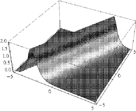
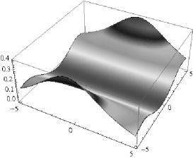
Figure 1: Exact soliton solutions (module) for the integrable a) homogeneous NLS (11) and b) inhomogeneous NLS (3) with $A=2.0,V=0.5$. and the particular choice $R=.008t^{2},D=1,s=0$. In spite of the significant differences between the appearance and dynamics of these two solutions they are related by simple transformations (7-9) and belong to equivalent integrable systems.

It is worth mentioning that, though in all earlier papers only 1-soliton of the IHNLS was considered, one can easily derive the exact N-soliton for the IHNLS, thanks to its complete integrability, by exploiting again its equivalence with the integrable NLS, i.e. by simply mapping the known N-soliton of the standard NLS through the same transformations (7-9).

By redefining the field further: $Q\to b(t)Qe^{ia(t)}$ with arbitrary functions $a(t),b(t)$, we can generate more inhomogeneous terms in (1) resulting a more general form of IHNLS

$$iQ_{t}+\frac{D}{2}Q_{xx}+R|Q|^{2}Q-(2\alpha x+{\Omega^{2}}x^{2}+a+i\gamma)Q=0,\ \ \gamma(t)=\frac{b_{t}}{b},$$ (12)

equivalent naturally to the integrable NLS. The IHNLS (12) was found to be the maximum inhomogeneous NLS system which can pass the Painlevé integrability criteria [11]. A recently proposed IHNLS [8], which is simply a particular case of (12) at $a=0$ and $\alpha=0$, is therefore also equivalent to the standard NLS and hence, contrary to the assumption in [8] that the system is only Painlevé integrable and not completely integrable, the equivalence with NLS assures the complete integrability, including the existence of infinite conserved quantities, N-soliton solutions etc. for this IHNLS [8]

We now look into other forms of integrable HNLS appeared earlier in Phys. Rev. [2, 3, 4] and PRL [1, 5, 6] and show their equivalence to the standard NLS, similar to as found above. The simplest form of inhomogeneity to the NLS: $2xq$ was proposed in [1], which is clearly a particular case of (3) with $\alpha=1,\Omega=0$, ensured by the choice $R=D=1,s=t$, proving thus its equivalence with the NLS.

A more general IHNLS with $F(x)Q$ was considered in [2] and shown finally that integrability restricts the choice only upto $F(x)=a+\alpha x+\mu x^{2}$, which is consistent with the general integrable IHNLS (12), shown to be equivalent to the standard NLS (11). However for constructing such integrable IHNLS, as shown here, x-dependent spectral parameter considered in [2] is not needed and similarly the restriction on function $h(t)$ appearing in $\lambda(t)$, found by the author apparently as a condition for the integrability, actually does not appear allowing the function to be arbitrary, as shown here.

In [5] a variant of IHNLS was considered, which was suspected to be integrable through computer simulation. It is easy to see however, that this IHNLS can be obtained as a particular case from (12) at $\alpha=0,s=1,a=0,\gamma=0,\Omega=0$, but with nontrivial $R(t),D(t),\gamma(t)$ obeying certain constraints. Similarly IHNLS proposed in [6] can be seen to be derivable from (12) as a particular case with $D=1,R(t)=g_{0}e^{ct},s=1,a=0,\gamma=0,$ giving $\alpha=0$, but $\Omega=-c^{2}$. Therefore both these inhomogeneous NLS [5, 6] are equivalent to the standard NLS and hence completely integrable.

Some integrable discrete versions of IHNLS, namely inhomogeneous Ablowitz-Ladik models (ALM) were proposed in [3, 4], containing in addition to the standard ALM [10] an inhomogeneous term $n\omega\psi_{n}$, with $\omega=1$ [3] or $\omega(t)$ as an arbitrary function [4] . We find that in spite of the discrete case a similar reasoning found here holds true and the proposed inhomogeneous ALM can be shown to be gauge equivalent to the standard ALM [10], under discrete gauge transformation: $\tilde{U}_{n}=g_{n+1}U_{n}g_{n}^{-1},\ \tilde{V}_{n}=g_{n}V_{n}g_{n}^{-1}+\dot{g}_{n}g_{n}^{-1},$ with $g_{n}=e^{-in\Gamma(t)\sigma^{3}}$ and redefinition of the field as $q_{n}\to\psi_{n}=q_{n}e^{i(2n+1)}\Gamma(t)$, where $\Gamma_{t}(t)=\omega(t)$ is an arbitrary function as found in [4].

Based on the above result we therefore conclude that the general inhomogeneous NLS, if integrable, should be of the form (12). Other forms of integrable IHNLS are only its particular cases. However all these inhomogeneous NLS are neither new nor independent integrable systems, but are equivalent to the standard homogeneous NLS, from which all their integrable structures like Lax pair, N-soliton solutions, infinite number of commuting conserved quantities etc. can be obtained easily through simple mapping. The time-dependent soliton amplitude, shape and velocity as well as the nonisospectral flow in these inhomogeneous NLS are just an artifact of the time-dependent coordinate, gauge and field transformations, needed to get these systems from the standard NLS. Therefore before proposing any new integrable inhomogeneous NLS the authors should check whether it can be linked in any way to the general integrable IHNLS (12), whose equivalence with the well known NLS we have proved here.

References

- [1] H. H. Chen and C. S. Liu, Phys. Rev. Lett. 37, 693 (1976)
- [2] R. Balakrishnan, Phys. Rev. A 32, 1144 (1985)
- [3] R. Scharf and A. R. Bishop, Phys. Rev. A 43, 6535 (1991);
- [4] V. V. Konotop, Phys. Rev. E 47, 1423 (1993); V. V. Konotop, O. A. Chubykalo and L. Vazquez, Phys. Rev. E 48, 563 (1993)
- [5] V. N. Serkin and A. Hasegawa, Phys. Rev. Lett. 85, 4502 (2000)
- [6] Z. X. Liang, Z. D. Zhang and W. M. Liu, Phys. Rev. Lett. 94, 050402 (2005)
- [7] V. N. Serkin, A. Hasegawa and T. L. Belyaeva, Phys. Rev. Lett. 98, 074102 (2007)
- [8] H. G. Luo et al , arXiv: 0808.3437 [nlin.PS]; H. G. Luo et al, arXiv: 0807.1192 [nlin.PS]
- [9] M. Ablowitz et al, Stud. Appl. Math. 53 294 (1974) M. Ablowitz and H. Segur, Solitons and Inverse Scattering Transforms (SIAM, Philadelphia, 1981) S. Novikov et al , Theory of Solitons (Consultants Bureau, NY, 1984)
- [10] M. Ablowitz , Stud. Appl. Math. 58 17 (1978)
- [11] N. Joshi, Phys. Lett A 125, 456 (1987)