Vector Meson Dominance as the first order
of a sequence of Padé Approximants

Abstract

The use of Padé Approximants for the analysis of the pion vector form-factor  is discussed and justified in this talk. The method is  tested first in a theoretical model  and applied then on real experimental data.  It is shown how the Padé Approximants  provide a convenient and reliable framework to incorporate both  low and high energy information in the euclidean region, leading to improved determinations  of the low energy parameters such as, e.g., the quadratic radius $\langle r^{2}\rangle^{\pi}_{V}$.

The object of the study of Ref. [2] was the pion vector form-factor (VFF), defined by

$$\langle\pi^{+}(p^{\prime})|\,J_{{}_{\rm E.M.}}^{\mu}\,|\pi^{+}(p)\rangle\,=\,(p+p^{\prime})^{\mu}\ F(Q^{2})\ ,$$ (1)

with the electromagnetic current $J_{{}_{\rm E.M.}}^{\mu}=\frac{2}{3}\overline{u}\gamma^{\mu}u-\frac{1}{3}\overline{d}\gamma^{\mu}d-\frac{1}{3}\overline{s}\gamma^{\mu}s$ and $Q^{2}\equiv-(p^{\prime}-p)^{2}$, such that $Q^{2}>0$ corresponds to space-like data.

Our knowledge on the VFF from the time-like experimental data tells us that the spectral function is essentially dominated by the vector resonance $\rho(770)$. The remaining effects are almost negligible. On the other hand, it is a well known fact that vector meson dominance (VMD) provides a good description of the space-like data up to relatively high energies.

The question raised in this work is not so much “why this is so” but rather “how can we make use of this knowledge”. Our aim is to construct a space-like description of the VFF that can be systematically improved. The Padé Approximants (PAs) provide this suitable framework.

A Padé Approximant to a given function is the ratio of two polynomials $R_{N}(z)$ and $Q_{M}(z)$ (with degree $N$ and $M$, respectively), constructed such that the Taylor expansion around some point (the origin in our case) exactly coincides with that of $F(z)$ up to the highest possible order, i.e. $F(z)-P^{N}_{M}(z)={\cal O}(z^{M+N+1})$. This may not look a big improvement with respect to the usual Taylor power expansion as they use the same inputs, the low energy coefficients. However, the polynomial is unable to handle singularities such as the logarithmic branch cut of the VFF, whereas they are partially mimicked by the Padé . Thus, in many cases the Padé works far beyond the range of applicability of Taylor expansions, allowing the incorporation of both low and high energy data. From this perspective, VMD, where $F(Q^{2})=(1+Q^{2}/M^{2}_{{}_{\rm VMD}})^{-1}$, is just a Padé $P_{1}^{0}$, the first term of a sequence of the form $P^{L}_{1}$.

Our analysis is focused on euclidean quantities in real Quantum Chromodynamics (QCD), i.e., with $N_{C}=3$. We separate away here from other studies based on QCD in the limit of large number of colours [3] where the large-$N_{C}$ amplitudes are approximated through rational functions [4, 5, 6]. In some situations, the poles and residues were real and could be related to hadronic masses and couplings. Instead, in the present work the Padés are just a useful mathematical tool which does not know about particles, masses, widths… Our aim is to describe the euclidean momentum range and doing that the Padés tend to mimic the shape of the physical spectral function -strongly peaked around the rho mass but finite- through a finite number of poles.

The traditional point of view with respect to VMD has been that the rho meson dominates, having the remaining resonances small couplings. As we said, the PAs do not care about the particle poles in the amplitude. The Padé poles rather seem to be more related to bumps in the spectral function than to hadronic poles (masses, widths, couplings…). The danger of relating the poles of the rational approximants with mesonic resonances is clear.

Obviously, unlike the space-like region, we do not expect to reproduce the time-like data since a PA contains only isolated poles and cannot recover a continuous time-like cut.

A final important point is that the PAs do not care about the asymptotic behaviour of the amplitude at very short distances. Although they work for a much wider range of momenta than a polynomial, the Padé eventually breaks down beyond some energy and they are not intended to reproduce the VFF at $Q^{2}\to\infty$.

The importance of these techniques is that they are able to produce alternative outcomes competitive with other approaches. The Padés are constructed in a simple and systematic way. They provide an efficient procedure which allows incorporating high-energy space-like information. This makes it an interesting alternative tool for the analysis of euclidean amplitudes.

There are several types of sequences of PAs that may be considered. In order to achieve a fast numerical convergence, the choice of which one to use is largely determined by the structure of the function to be approximated. In this regard, a glance at the time-like data of the pion form factor makes it obvious that the form factor is clearly dominated by the rho meson contribution. The effect of higher resonance states, although present, is much more suppressed. In these circumstances the natural choice is a single-pole Padé sequence $P^{L}_{1}$ [7], i.e. the ratio of a polynomial of degree $L$ over a polynomial of degree one. Nonetheless, one should not confuse the Padé pole with the rho mass.

In order to test the aforementioned single-pole dominance, we have also considered the sequence $P^{L}_{2}$, confirming the results found with the PAs $P^{L}_{1}$. We have also considered the so-called Padé-Type approximants (PTs) [5, 8] (rational approximants whose poles are fixed beforehand; here they have been taken to be the physical masses). Finally, we also considered an intermediate case, the so-called Partial-Padé approximants (PPs) [8], in which some of the poles are fixed to the physical masses and some are left free and fitted. The different results were rather independent of the kind of rational approximant used, being all of them consistent among themselves.

Test with a model

In order to illustrate the usefulness of the PAs, we will first use a phenomenological model as a theoretical laboratory to check our method.

A VFF phase-shift with the right threshold behaviour is considered [9, 10, 11]:

$$\delta(t)=\arctan\left[\frac{\hat{M}_{\rho}\hat{\Gamma}_{\rho}(t)}{\hat{M}_{\rho}^{2}-t}\right]\ ,$$ (2)

with the $t$-dependent width given by [9, 10]

$$\hat{\Gamma}_{\rho}(t)=\Gamma_{0}\ \left(\frac{t}{\hat{M}_{\rho}^{2}}\right)\ \frac{\sigma^{3}(t)}{\sigma^{3}(\hat{M}_{\rho}^{2})}\ \theta\left(t-4\hat{m}_{\pi}^{2}\right)\ ,$$ (3)

and $\sigma(t)=\sqrt{1-4\hat{m}_{\pi}^{2}/t}$. The input parameters are chosen to be close to their physical values $\Gamma_{0}=0.15$ GeV, $\hat{M}_{\rho}^{2}=0.6$ GeV², $4\hat{m}_{\pi}^{2}=0.1$ GeV². The form-factor is then recovered through a once-subtracted Omnés relation,

$$F(Q^{2})=\exp\left\{-\frac{Q^{2}}{\pi}\int_{4\hat{m}_{\pi}^{2}}^{\infty}\ dt\ \frac{\delta(t)}{t(t+Q^{2})}\right\}\ .$$ (4)

At low energies, the form-factor is given by the Taylor expansion,

$$F(Q^{2})\,=\,1\,+\,\sum_{k=1}^{\infty}a_{k}\,(-Q^{2})^{k}\,\,,$$ (5)

where the coefficients $a_{k}$ are known since they are determined by $\Gamma_{0}$, $\hat{M}_{\rho}^{2}$ and $4\hat{m}_{\pi}^{2}$. The condition $F(0)=1$ has been already incorporated.

In order to recreate the experimental situation [12]-[17], an emulation of the space-like experimental data is generated in the range $0.01$ GeV${}^{2}\leq Q^{2}\leq 10$ GeV² [2].

The Padé Approximants $P^{L}_{1}(Q^{2})$ are then fitted to these euclidean “data” points, providing a prediction for the low-energy coefficients $a_{k}$. It is found that as L increases the sequence of PAs $P^{L}_{1}$ converges to the exactly known results, although in a hierarchical way, i.e. much faster for $a_{1}$ than for $a_{2}$, and this one much faster than $a_{3}$, etc… The relative error achieved in determining the coefficients $a_{k}$ by the Padé $P^{4}_{1}$ was, respectively, $1.5\%$ and $10\%$ for $a_{1}$ and $a_{2}$. These results will be taken as a rough estimate of the systematic uncertainties when fitting the real experimental data with Padés in next section, and they will be added to the final error [2].

Experimental data analysis

All the available experimental data in the space-like region have been employed [12]-[17], ranging in momentum from $Q^{2}=0.015$ up to 10 GeV².

As discussed in the introduction, the prominent role of the rho meson contribution motivates that we start with the $P^{L}_{1}$ Padé sequence.

Figure 1: The sequence of $P^{L}_{1}$ PAs is compared to the available space-like data [12]-[17]: $P^{0}_{1}$ (brown dashed), $P^{1}_{1}$ (green thick-dashed), $P^{2}_{1}$ (orange dot-dashed), $P^{3}_{1}$ (blue long-dashed), $P^{4}_{1}$ (red solid).

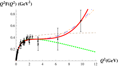
The fit to $P^{L}_{1}$ yields a determination for the pion VFF and the coefficients $a_{k}$. Nonetheless, according to Ref. [18], the VFF is supposed to fall like $1/Q^{2}$ (up to logarithms) for $Q^{2}\to\infty$. This means that, for any given value of $L$, one may expect a good fit only up to a finite value of $Q^{2}$, but not for asymptotically large momentum. This is clearly seen in Fig. 1, where the Padé sequence $P^{L}_{1}$ is compared to the space-like data. The Padés converge to the real VFF at low and mid energies but eventually diverge.

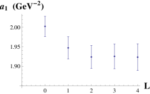
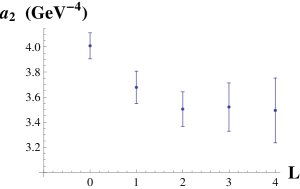
Fig. 2 shows the evolution of the fit results for the Taylor coefficients $a_{1}$ and $a_{2}$. As one can see, after a few Padés they become stable [2]. Thus, our best fit is provided by $P_{1}^{4}$ [2], yielding

$$\begin{array}[]{c}a_{1}\,=\,1.92\pm 0.03\,\,\mbox{GeV}^{-2}\,,\\ a_{2}\,=\,3.49\pm 0.26\,\,\mbox{GeV}^{-4}\,,\end{array}$$ (6)

with a $\chi^{2}/\mathrm{dof}=117/90$.

Figure 2: $a_{1}$ and $a_{2}$ Taylor coefficients for the $P^{L}_{1}$ PA sequence.

Alternative rational approximations were also constructed [2]: two-pole PAs, Padé-Types and Partial-Padés [5]. They all provided compatible results.

Conclusions

Table 1: Our results for the quadratic radius $\langle r^{2}\rangle_{V}^{\pi}$ and second derivative $a_{2}$ are compared to other determinations [11, 19, 20, 21, 22, 23]. Our first error is statistical. The second one is systematic, based on the analysis of the VFF model of the previous section [2].

	$\langle r^{2}\rangle_{V}^{\pi}$ (fm2)	$a_{2}$ (GeV-4)
This work [2]	$0.445\pm 0.002_{\mathrm{stat}}\pm 0.007_{\mathrm{syst}}$	$3.30\pm 0.03_{\mathrm{stat}}\pm 0.33_{\mathrm{syst}}$
CGL [19, 20]	$0.435\pm 0.005$	…
TY [21]	$0.432\pm 0.001$	$3.84\pm 0.02$
BCT [22]	$0.437\pm 0.016$	$3.85\pm 0.60$
PP [11]	$0.430\pm 0.012$	$3.79\pm 0.04$
Lattice [23]	$0.418\pm 0.031$	…

Combining all these outcomes, we obtained the results shown in Table 1. For comparison with previous analyses, the value of the quadratic radius is provided (given by $\langle r^{2}\rangle_{V}^{\pi}\,=\,6\,a_{1}$, with our best determination $a_{1}=1.907\pm 0.010_{{}_{\rm sta}}\pm 0.03_{{}_{\rm sys}}$ GeV^-2).

In summary, in this work we have used rational approximations as a tool for fitting the pion vector form factor in the euclidean range. Since these approximants are capable of going beyond the low-energy region, they are rather suitable for the description of space-like data. They allow to extract the low-energy coefficients, improving on their determination by incorporating also the euclidean high-energy data information. As one can see in Table 1, the achieved degree of uncertainty is shown to be competitive with previous analyses existing in the literature [11, 19, 20, 21, 22, 23].

References

- [1]
- [2] P. Masjuan et al. [arXiv:0807.4893 [hep-ph]].
- [3] G. ’t Hooft, Nucl. Phys. B 72 (1974) 461; 75 (1974) 461; E. Witten, Nucl. Phys. B 160 (1979) 57.
- [4] S. Peris, Phys. Rev. D 74 (2006) 054013; P. Masjuan and S. Peris, JHEP 0705 (2007) 040.
- [5] P. Masjuan and S. Peris, Phys. Lett. B 663 (2008) 61.
- [6] A. Pich, [arXiv:hep-ph/0205030].
- [7] G.A. Baker and P. Graves-Morris, Padé Approximants, Encyclopedia of Mathematics and its Applications, Cambridge Univ. Press. 1996; chapter 3, sections 3.1 and 3.2; C. Bender and S. Orszag, Advanced Mathematical Methods for Scientists and Engineers I: asymptotic methods and perturbation theory, Springer 1999, section 8.6.
- [8] C. Brezinski and J. Van Inseghem, Padé Approximations, Handbook of Numerical Analysis, P.G. Ciarlet and J.L. Lions (editors), North Holland, vol. III. See also, e.g., C. Diaz-Mendoza et al., Appl. Num. Math. 53 (2005) 39 and references therein.
- [9] F. Guerrero and A. Pich, Phys. Lett. B 412 (1997) 382-388.
- [10] D. Gomez Dumm et al., Phys. Rev. D 62 (2000) 054014; J. J. Sanz-Cillero and A. Pich, Eur. Phys. J. C 27 (2003) 587.
- [11] A. Pich and J. Portolés, Phys. Rev. D 63 (2001) 093005.
- [12] S.R. Amendolia et al. (NA7 Collaboration), Nucl. Phys. B 277 (1986) 168.
- [13] V. Tadevosyan et al. (JLab F(pi) Collaboration), Phys. Rev. C 75 (2007) 055205;
- [14] T. Horn et al. (JLab F(pi)-2 Collaboration), Phys. Rev. Lett. 97 (2006) 192001; T. Horn et al. (JLab) [arXiv:0707.1794 [nucl-ex]].
- [15] C. N. Brown et al., Phys. Rev. D 8 (1973) 92; C. J. Bebek et al., Phys. Rev. D 9 (1974) 1229; C. J. Bebek et al., Phys. Rev. D 13 (1976) 25; C. J. Bebek et al., Phys. Rev. D 17 (1978) 1693.
- [16] P. Brauel et al., Z. Phys. C3, 101 (1979).
- [17] Dally et al., Phys. Rev. Lett. 39 (1977) 1176.
- [18] G. P. Lepage and S. J. Brodsky, Phys. Lett. B 87 (1979) 359; Phys. Rev. D 22 (1980) 2157; Phys. Rev. D 24 (1981) 1808.
- [19] H. Leutwyler, [arXiv:hep-ph/0212324]; G. Colangelo, Nucl. Phys. Proc. Suppl. 131 (2004) 185-191.
- [20] G. Colangelo, J. Gasser and H. Leutwyler, Nucl. Phys. B 603 (2001) 125.
-
[21]
J.F. de Troconiz and F.J. Yndurain,
Phys. Rev. D 65 (2002) 093001; Phys. Rev. D 71 (2005) 073008. - [22] J. Bijnens, G. Colangelo and P. Talavera, JHEP 05 (1998) 014.
- [23] P. A. Boyle et al., arXiv:0804.3971 [hep-lat].