Influence of the atomic-scale inhomogeneity of the pair interaction on extracted from the STM spectra characteristics of high-$T_{c}$ superconductors.

Abstract

The influence of the atomic-scale inhomogeneities of the pairing interaction strength on the superconducting order parameter and the conductance spectra measurable by STM is studied in the framework of weak-coupling BCS-like theory for two-dimensional lattice model. First of all, it is found that the inhomogeneity having the form of atomic-scale regions of enhanced pair interaction increases the ratio of the local low-temperature gap in differential conductance spectra to the local temperature of vanishing the gap $2\Delta_{g}/T_{p}$. Even in the framework of mean-field treatment this ratio is shown to be larger than the one corresponding to the homogeneous case. It is shown that the effect of thermal phase fluctuations of the superconducting order parameter can further increase this ratio. Taking them into account in the framework of a toy model we obtained the ratio $2\Delta_{g}/T_{p}$ to be $\sim 7-8$. It is found that the additional atomic-scale hopping element disorder and weak potential scatterers, which can also take place in cuprate materials, have no considerable effect on the statistical properties of the system, including the distribution of the gaps, $T_{p}$ and the ratio $2\Delta_{g}/T_{p}$. The second consequence of the atomic-scale order parameter inhomogeneity is the anticorrelation between the low-temperature gap and the high-temperature zero-bias conductance. The obtained results could bear a relation to recent STM measurements.

I Introduction

Nanoscale inhomogeneities have been widely observed in the high-temperature superconductor $\rm Bi_{2}Sr_{2}CaCu_{2}O_{8+x}$ (BSCCO) and have generated intense interest cren00 ; pan01 ; howard01 ; lang02 ; mcelroy05 ; fang06 . In particular, the spectral gap in the local density of states (LDOS) has been investigated by scanning tunneling microscopy (STM). It was found that deeply in the superconducting state the low-temperature gap varies by a factor of 2 over distances of $20-30$ $\overset{\circ}{\rm A}$. Recently the existence of very similar picture of inhomogeneities in $La_{2-x}Sr_{x}CuO_{4}$ has been also reported kato08 . Several scenarios have been proposed to understanding this electronic inhomogeneity. First of all, it was speculated that poorly screened electrostatic potentials of the dopant atoms vary a doping concentration locally, giving rise to the gap modulations martin01 ; zwang02 ; qwang02 ; zhou06 . Alternatively, these inhomogeneities are associated with a competing order parameter, such as spin kivelson03 ; atkinson05 ; alvarez05 and orbital antiferromagnetism ghosal04 , charge density wave podolsky03 or pair density wave chen04 . Further, the positive correlations between the inhomogeneities and positions of the dopant atoms have been observed by STM on the optimally doped BSCCO mcelroy05 . After that it was proposed by Nunner et al. in Ref. nunner05, that the dopant atoms modulate the pairing interaction locally on the atomic scale. The LDOS calculated in the framework of this model is in good agreement with the key characteristics of the experimental spectra. However, there is an alternative picture of the inhomogeneity origin based on the local variation of the doping concentration, which explains why the correlations are rather weak zhou06 .

On the other hand, in the high-$T_{c}$ superconductors a partial gap in the LDOS exists for a range of temperatures above $T_{c}$ timusk99 . There is no consensus up to now if this gap is due to pairing without phase coherence, a competing order or proximity to the Mott state norman05 ; lee06 ; millis06 ; cho06 . The inhomogeneities described above complicate the situation. Only very recently the spatially resolved STM measurements of gap formation in BSCCO samples with different $T_{c}$ corresponding to hole concentrations from $0.12$ to $0.22$ were performed gomes07 . For a range of doping from $0.16$ to $0.22$ they have found that gaps nucleate in nanoscale regions above $T_{c}$ and proliferate as the temperature is lowered, evolving to the spatial distribution of gap values in the superconducting state. It was observed experimentally that overdoped and optimally doped samples have identical gap-temperature scaling ratios. Taking into account this finding together with the fact that in the overdoped samples pseudogap effects are believed to be weak or absent and consistency of the low-temperature spectra with a $d$-wave superconducting gap, Gomes $\it et.al$gomes07 have interpreted the gaps above $T_{c}$ as those associated with pairing. Despite the inhomogeneity, every pairing gap develops locally at the temperature $T_{p}$ following the relation $2\Delta_{g}/T_{p}=7.9\pm 0.5$ in wide range of doping from overdoped to optimally doped samples. This local pairing criterion seems to fail only in underdoped samples and DOS indicates the presence of another phenomenon, possibly unrelated to pairing.

It is well-known that in the framework of weak-coupling BCS theory with homogeneous pairing amplitude the ratio $2\Delta_{g}/T_{c}$ is $3.5$ for $s$-wave superconductors and approximately is in the interval $4.3-4.5$ for d-wave superconductors (this value depends slightly on the particular tight-binding parameters). The ratio $2\Delta_{g}/T_{p}\sim 4.7-5.2$ for d-wave case is a bit higher due to thermal smearing of the measured dI/dV curves. It is worth to note that in the framework of strong-coupling theory the ratio $2\Delta_{g}/T_{c}$ is in the range $3.5-5$ for s-wave superconductors, but becomes dependent on $\Delta_{g}$ and can reach the values $\sim 10$ for d-wave pairing case scalapino94 .

In the present paper we show that if the superconducting order parameter (OP) is modulated locally on the atomic scale, the ratio $2\Delta_{g}/T_{p}$ strongly increases in the framework of conventional weak-coupling theory. In addition, this inhomogeneity inevitably leads to the anticorrelation between the low-temperature gap and the high-temperature zero-bias conductance. This findings resemble the results observed in recent STM experimentsgomes07 ; yazdani08 . The most natural way to obtain the atomic-scale modulations of the OP is to assume the atomic-scale modulations of the pairing interaction strength, as it was proposed by Nunner et. al nunner05 . We do not mean any particular mechanism of pairing. Our analysis is phenomenological and the conclusions are independent on the underlying pairing mechanism and the particular course of the local pair interaction modulations. Here we only focus on the effect of the inhomogeneity on some observable properties of cuprate superconductors. As it is discussed below, if this inhomogeneity has the form of atomic-scale regions of enhanced pair interaction, the ratio $2\Delta_{g}/T_{p}$ increases even in the framework of mean-field treatment. However, the effect only takes place if the total area of these regions is less than the area occupied by the background interaction. The last condition is essential. If this is not the case, that is the total area of the enhanced pairing regions is of the order of or larger than the area of the background pairing, the discussed ratio is reduced or, at least, remains equal to the homogeneous one. It was demonstrated in a number of papers. In particular, the attractive Hubbard model with inhomogeneous pairing amplitude was studiedaryanpour and it was shown that the superconducting critical temperature can be significantly increased in such a system as compared to a uniform system corresponding to the pairing interaction averaged over the system. The zero temperature superconducting order parameter increases also, but in a less degree than the critical temperature, what results in reducing the ratio $2\Delta_{g}/T_{c}$. The reduction of the ratio of the energy gap to the critical temperature due to the inhomogeneity of coupling constant was also obtained for dirty s-wave superconductorszou07 . The potential disorder, as was demonstrated franz97 , also diminishes this quantity because the superconducting order parameter is suppressed on the distance of the order of the coherence length around an impurity and, consequently, the total area of the enhanced order parameter regions dominates.

Further, it is physically reasonable that the phase of the superconducting order parameter should fluctuate from one region of enhanced pairing amplitude to another in such an inhomogeneous situation, especially for short coherence length cuprate superconductors. In particular, the state with antiferromagnetic and nano-scale superconducting domains exhibiting randomly distributed phases was recently proposed alvarez08 to account for the formation of the Fermi arcs, observed in the pseudogap phase of the underdoped cupratesnorman98 ; kanigel06 ; kanigel07 . The existence of the thermal phase fluctuations of the superconducting clustered state in disordered s-wave superconductors and their role in the superconductor-insulator transition was demonstrateddubi07 . In the present paper we show that thermal phase fluctuations can significantly suppress the temperature $T_{p}$ and, consequently, increase the ratio $2\Delta_{g}/T_{p}$. Even in the framework of very simple model we study here this quantity reaches the value $\sim 7-8$, comparable to the experimentally observedgomes07 .

The influence of the additional disorder such as the atomic-scale inhomogeneities of the hopping matrix elements and weak potential scatterers is also considered. It is shown that while they can affect the shape of low-temperature LDOS in the system, the properties of interest: gap’s distribution, $T_{p}$’s distribution and the distribution of the ratio $2\Delta_{g}/T_{p}$ remain qualitatively unchanged.

The paper is organized as follows. Sec. II is devoted to the detailed mean-field consideration of the problem. The model mean-field Hamiltonian we use and the outline of the T-matrix method are introduced in Sec. II.1. The single pair interaction perturbation is studied and the physical reasons for the enhancement of the ratio $2\Delta_{g}/T_{p}$ are discussed in Sec. II.2. Sec. II.3 is devoted to the mean-field treatment of the interaction between many OP scatterers. The effect of additional weak potential and hopping element inhomogeneities is investigated in Sec. II.4. The influence of the thermal phase fluctuations on the quantities under consideration is discussed in Sec. III. In Sec. IV it is demonstrated that the atomic-scale OP inhomogeneity leads to the anticorrelation between the local low-temperature gap and the value of zero-bias conductance at higher temperatures. The conclusions are presented in Sec. V.

II Mean-field treatment

II.1 Model and method

We consider the following Hamiltonian on a square lattice

$$\hat{H}=-\sum\limits_{ij,\sigma}t_{ij}c_{i\sigma}^{\dagger}c_{j\sigma}-\sum\limits_{i,\sigma}\mu c_{i\sigma}^{\dagger}c_{i\sigma}+\sum\limits_{\langle ij\rangle}\left(\Delta_{ij}c_{i\uparrow}^{\dagger}c_{j\downarrow}^{\dagger}+h.c.\right)\enspace,$$ (1)

where $c_{i\sigma}(c_{i\sigma}^{\dagger})$ stands for an electron annihilation (creation) operator at site $i$ with spin $\sigma$. $\sum_{ij}$ indicates summation over neighboring sites, while $\sum_{\langle ij\rangle}$ denotes the summation over nearest neighbors. $t_{ij}$ is the hopping integral between sites $i$ and $j$. We set $t_{ij}$ to be $t=1$ for the nearest-neighbor hopping and all the energies are measured in units of $t$ throughout the paper. The nearest-neighbor $d$-wave order parameter should be determined self-consistently: $\Delta_{ij}=-g_{ij}\langle c_{i\downarrow}c_{j\uparrow}-c_{j\downarrow}c_{i\uparrow}\rangle$.

In order to analyze the inhomogeneous pairing correlations in the framework of the mean-field Hamiltonian (1) we exploit the fully self-consistent T-matrix technique for Gor’kov Green’s functions. Starting from the Gor’kov equations the normal and anomalous Green’s functions are expressed in terms of the homogeneous background Green’s functions $\check{G}_{ij}^{0}$ and the T-matrix, which contains all the inhomogeneities. Then the full Green’s function, which depends on two space indices $i$ and $j$, takes the form

$$\check{G}_{ij}=\check{G}_{ij}^{0}+\sum\limits_{k,m}\check{G}_{ik}^{0}\check{T}_{km}\check{G}_{mj}^{0}\enspace.$$ (2)

Here $\check{T}_{km}=-\sum\limits_{n}(\check{M}^{-1})_{kn}\check{V}_{nm}$, $\check{M}_{km}=\delta_{km}+\sum\limits_{n}\check{G}_{kn}^{0}\check{V}_{nm}$. $\check{V}_{km}$ is the perturbation matrix including all the inhomogeneities. All Green’s functions and T-matrices are $4\times 4$ matrices in the direct product of spin and particle-hole spaces, what indicated by the symbol $\check{~}{}$. $\hat{\tau}_{i}$ and $\hat{\sigma}_{i}$ are Pauli matrices in particle-hole and spin spaces, respectively. The summation is taken over all the sites, where the OP $\Delta_{km}=\Delta_{km}^{0}+\delta\Delta_{km}$ differs from the background value $\Delta_{km}^{0}$. $\Delta_{km}^{0}$ is assumed to be of $d$-wave type, that is $\Delta_{ii\pm\hat{a}}^{0}=-\Delta_{ii\pm\hat{b}}^{0}=\Delta^{0}$. $\hat{a}$ and $\hat{b}$ are basis vectors of the square lattice. We set the lattice constant $a$ to be equal to unity.

OP is to be calculated from the self-consistency equation

$$\Delta_{ij}=g_{ij}T\sum\limits_{\varepsilon_{n}}{\rm Tr}_{4}\left[\hat{\tau}_{-}i\hat{\sigma}_{y}\check{G}_{ij}(\varepsilon_{n})\right]\enspace,$$ (3)

where $\hat{\tau}_{-}=(\hat{\tau}_{x}-i\hat{\tau}_{y})/2$ and $\varepsilon_{n}$ is the fermionic Matsubara frequency. The energy cutoff $|\varepsilon_{n}|<4$ is used in Eq. (3) for the technical convenience. We have checked that the particular value of the cutoff energy (if it is considerably larger than the maximal value of the OP) does not change qualitatively the results and only slightly varies the OP quantitative values. Eqs. (3) and (2) allow us to find the OP $\Delta_{ij}$ numerically. Making use of the outlined technique we consider a square of the size $n\times n$, immersed into an infinite lattice carrying the homogeneous OP $\Delta^{0}_{ij}$, as an inhomogeneity described by T-matrix.

II.2 Single perturbation

In general, the T-matrix can describe inhomogeneities of all the parameters entering the equations: hopping elements, chemical potential or self-energies. For the moment we only focus on the off-diagonal self-energy inhomogeneity and therefore $\check{V}_{km}=\delta\Delta_{km}i\hat{\sigma}_{2}i\hat{\tau}_{2}$. We begin by considering a single perturbation of the pairing interaction. Two different models for the individual pairing perturbation are represented in the paper. Model (a) describes the region of the enhanced pair interaction emanating from a site $i$ by Yukawa-type potential $g_{ij}=g_{b}+\delta gf_{ij}$, where $g_{b}$ corresponds to a background interaction and $f_{ij}=\sum_{s}\exp(-r_{ijs}/\lambda)/r_{ijs}$. $r_{ijs}=\sqrt{r_{ijs}^{(ab)2}+z^{2}}$ is the distance between the center of the bond connecting the sites $i$ and $j$ and the source of the pairing interaction perturbation beyond the plane. Here $z$ is the distance between the ${\rm CuO}_{2}$ plane and the source of the perturbation and $r_{ijs}^{(ab)}$ denotes the distance in the plane. Model (b) supposes that the pair interaction is considerably enhanced on a plaquette and has a long weak tail beyond this plaquette: $g_{ij}=g_{b}+u_{1}$ if the bond $ij$ belongs to the chosen plaquette and $g_{ij}=g_{b}+u_{2}/(r_{0,ij}^{2}+z^{2})$ if the bond $ij$ is beyond this plaquette. Here, $r_{0,ij}$ is the distance between the center of the chosen plaquette and the center of the bond $ij$. By considering a number of different models for the single perturbation we have checked that the results do not depend qualitatively on the particular shape of the perturbation and are only controlled by its effective width and height. The tight binding model parameters taken to obtain the normal quasiparticle dispersion are the following: the next-nearest neighbor hopping $t^{\prime}=-0.3$ and the chemical potential $\mu=-1$ correspond to the normal state background of model (a) and $t^{\prime}=-0.35$ and $\mu=-0.8$ describe the normal background of model (b). Both sets of the parameters give approximately the same low-energy dispersion and adjust to qualitatively reproduce experimentally measured Fermi surface of BSCCO near optimal doping. However, they result in quite different quasiparticle dispersions for the energies, which have the absolute value of the order of superconducting gap, and, in particular, differ by the energy location of the normal state van Hove singularity $\varepsilon_{vH}=-\mu+4t^{\prime}$. This fact leads to essential difference in the shape of the LDOS curves, but does not influence qualitatively the statistical properties considered here: gap ($\Delta_{g}$) distribution, the local temperature of vanishing the gap ($T_{p}$) distribution and the ratio $2\Delta_{g}/T_{p}$. We comment on the role of the particular set of tight binding model parameters in more detail below. Making use of the $T$-matrix approach outlined above we calculate the superconducting order parameter, local density of states and $T_{p}$ for the two inhomogeneous patterns with a single perturbation described by models (a) and (b), respectively.

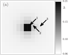
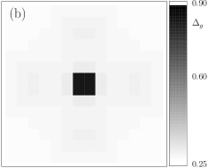
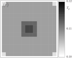
The resulting space distributions of low-temperature site-averaged OP $\Delta_{i}\equiv(\Delta_{i,i+\hat{a}}+\Delta_{i,i-\hat{a}}+|\Delta_{i,i+\hat{b}}|+|\Delta_{i,i-\hat{b}}|)/4$ are presented in Figs. 1(a) and 2(a) for models (a) and (b), respectively.

Figure 1: (a) Low-temperature ($T=0.03$) distribution of the site-averaged OP. (b) Low-temperature ($T=0.03$) gap map. (c) $T_{p}-$map. (d) The space profiles of the ratio $2\Delta_{g}/T_{p}$ (solid line) and the site-averaged OP (dashed line) calculated along the horizontal line drawn though the center of the perturbation in panel (a). The left (right) vertical axis corresponds to the ratio $2\Delta_{g}(i)/T_{p}(i)$ (superconducting order parameter). All the pictures correspond to the single perturbation described by model (a) (see text) with $g_{b}=0.51$, $\delta g=2.09$, $\lambda=1.5$ and $z=1.5$. The parameters $\lambda$ and $z$ are measured in units of the lattice constant $a$.

Figure 2: The panels (a)-(d) represent the same quantities as in Fig. 1, but correspond to the single perturbation described by model (b) (see text) with $g_{b}=0.59$, $u_{1}=1.00$, $u_{2}=0.25$ and $z=0.5$.

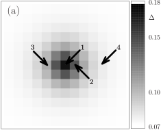
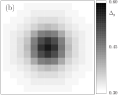
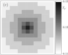
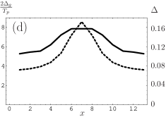
STM technique measures the local differential conductance, and the thermally smeared LDOS, described by the expression

$$dI/dV\sim\int\limits_{-\infty}^{\infty}d\varepsilon\frac{df(\varepsilon+V)}{dV}\rho_{i}(\varepsilon,T)\enspace,$$ (4)

can be extracted from these measurements. We set $|e|=1$ throughout the paper. In the above expression

$$\rho_{i}(\varepsilon,T)=-(1/\pi){\rm Im}G_{ii}^{R}(\varepsilon,T)$$ (5)

is the local density of states, $f(\varepsilon)$ is Fermi distribution function and $V$ is voltage applied between the STM tip and the sample. For the homogeneous situation the distance between the coherence peaks $2\Delta_{g}$ in the low-temperature conductance spectra is directly connected to the low-temperature OP by the simple relation $\Delta_{g}=\alpha\Delta_{0}(T)$, where the parameter $\alpha$ is slightly model dependent. In our case $\alpha=4.0$ for model (a) and $\alpha=3.6$ for model (b).

For an inhomogeneous system, where the characteristic size of the patch $\lesssim\xi$, there is no any direct simple relationship between the local OP and the local gap $\Delta_{g}$. One can only conclude from the numerical calculations nunner05 ; fang06 that for regions, where the OP is enhanced from the background, the gap gets wider and the peak height is suppressed compared to the average value. It is worth noting that, unlike the homogeneous situation, this peak does not always represent the maximal superconducting gap on the Fermi surface, but in some cases originates from the spectral weight transfer from the nearby van Hove singularity due to the Andreev scattering processes. Otherwise, if the OP in a cluster is less than that one in the background, the narrow and high Andreev resonant peaks develop in the cluster region resulting in diminishing of the gap region. For this reason we investigate not only the OP distribution, but also the experimentally measurable thermally smeared LDOS, which has a maximum at $V=\Delta_{g}$. For models (a) and (b) of the single perturbation the corresponding low-temperature gap maps are represented in Figs. 1(b) and 2(b), respectively.

Experimentally gomes07 the temperature $T_{p}(i)$ of the gap disappearing for the particular location in the sample has been determined using the criterion $dI/dV(V=0)\geq dI/dV$ (for all $V\geq 0$). Using the above criterion we calculated the distribution $T_{p}(i)$ from the thermally smeared LDOS curves. The corresponding $T_{p}$-maps for the single perturbations described by models (a) and (b) are represented in Fig. 1(c) and 2(c), respectively. It can be seen from Figs. 1 and 2 that while the space distribution of the superconducting order parameter mainly follows that one of the pairing interaction strength due to the local multiplication of the anomalous Green’s function in the self-consistency equation (3) by the coupling constant, LDOS and $T_{p}$ are essentially nonlocal (on the atomic scale) quantities with the characteristic size of order of $\xi_{s}$ determined by the scale, where the Green’s functions change considerably. This is valid for the both considered models, however the non-locality is much less pronounced for model (b). The reason is that the pair interaction perturbation is more spikier in this case as compared to model (a). Due to its very small effective width the perturbation (b) cannot contribute considerably to the Green’s function and, consequently, to the LDOS anywhere in space except for its own plaquette. The reason for enhancement of the gap at this plaquette is spectral weight transfer from the nearby Van Hove singularity, which is discussed in detail later.

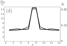
The ratios $2\Delta_{g}(i)/T_{p}(i)$ calculated along the horizontal lines drawn through the centers of the perturbations in Figs. 1(a) and 2(a) for the model samples considered above are plotted in Figs. 1(d) and 2(d) together with the spacial profiles of the superconducting order parameter along the same cuts. It is seen that this ratio is considerably enhanced in comparison with the homogeneous situation. For model (a) the area of the enhancement is larger that the characteristic size of the superconducting order parameter (and coupling constant) perturbation. This is due to the above mentioned gap and $T_{p}$ nonlocality and leads to the increasing of the ratio over the entire sample in the situation with many off-diagonal scatterers in spite of the fact that only smaller part of the sample is occupied by the enhanced coupling constant regions. On the contrary, for model (b) the two profiles practically coincide. Note that the maximal ratio is very high ($\sim 14$) for this model. The physical reasons for this fact will be given later. The averaged ratio $\langle 2\Delta_{g}(i)/T_{p}(i)\rangle$ calculated over the region of the size, which approximately corresponds to the average distance between the centers of enhanced pairing regions in the situation with many individual perturbations considered below, is equal to $7.6$ and $8.5$ for models (a) and (b), respectively.

There are two main physical reasons for the enhancement of the ratio $2\Delta_{g}/T_{p}$ for the single perturbation considered above. First of all, small as compared to superconducting coherence length perturbations cannot maintain superconductivity by themselves and only do this due to the superconductivity in the bulk. Although the value of the zero-temperature OP strongly increases when the height of the perturbation grows, at finite temperatures where the bulk OP vanishes, the pairing correlations in the small area go to zero abruptly. To illustrate this the dependence of the site-averaged OP on temperature is presented in Fig.3. Panels (a) and (b) correspond to models (a) and (b) described above. The bottom thin line represents the temperature dependence of the background order parameter generated by the coupling constant $g_{b}$. The bold solid curves correspond to the temperature dependence of the site-averaged order parameter for the sites marked by the appropriate numbers in Figs. 1(a) and 2(a), respectively. Although the superconducting order parameter vanishes at the critical temperature denoted by $T_{x}$ over the entire inhomogeneous sample simultaneously, as it should be in the mean-field approximation, the pairing correlations in the small area reduce abruptly near the temperature of the vanishing of the bulk OP corresponding to the coupling constant $g_{b}$. Then only the non BCS-like tails extend up to $T_{x}$. In other words, the OP inside the area of the enhanced pair interaction disappear with temperature more faster than the bulk OP having the same low-temperature value. To demonstrate this the temperature dependence of the bulk OP having the same low-temperature value as in the center of the perturbation (curves marked by $1$) is depicted by the upper thin lines in Figs. 3(a) and (b). Note that for model (b) the abrupt suppression of the OP near the background critical temperature $T_{b}$ is seen more clearly due to smaller effective size of the perturbation.

Figure 3: Dependence of the site-averaged OP on temperature for the single perturbation. The thin bottom line corresponds to bulk order parameter generated by the background coupling constant. The bold solid curves represent the temperature dependence of the superconducting order parameter for the sites marked by the appropriate numbers in Fig. 1(a) and 2(a). The upper thin line is the temperature dependence of the bulk OP with the same zero-temperature value as in the center of the perturbation (curve marked by $1$). The panels (a) and (b) correspond to the models (a) and (b), respectively.

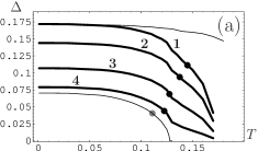
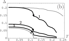
The temperatures $T_{p}$ of vanishing the gap for the given space locations are marked by the filled circles on the corresponding $\Delta(T)$ curves in Figs. 3(a) and (b). It is seen that even for the homogeneous case $T_{p}$ is slightly lower than the critical temperature (see the bottom thin line) due to the thermal smearing of the measured differential conductance according to the formula (4). Consequently, the bulk ratio $2\Delta_{g}/T_{p}$ is a bit higher than the ratio $2\Delta_{g}/T_{b}$. These ratios are dependent slightly on the particular coupling constant and tight-binding parameters. For model (a) we consider they have the following values: $(2\Delta_{g}/T_{b})^{(a)}=4.4$ and $(2\Delta_{g}/T_{p})^{(a)}=5.0$, while for model (b) $(2\Delta_{g}/T_{b})^{(b)}=4.2$ and $(2\Delta_{g}/T_{p})^{(b)}=4.7$. For the inhomogeneous situation with the single perturbation the difference between $T_{x}$ and $T_{p}$ ($T_{p}$ is now position dependent) is much more pronounced. This results from the discussed above non BCS-like behavior of the OP on temperature: for the long OP tails, taking place for the temperatures higher than the background critical temperature, the gap is too small and easily smeared out by high enough temperature. Although at the center of the perturbation the value of the superconducting OP is still high enough at the temperatures of the order of $T_{p}$, the area occupied by this enhanced OP is small as compared to $\xi_{s}^{2}$. Consequently, the amplitude of the corresponding peak in the LDOS is low and again can be easy washed out by temperature. These reasons work more efficiently for more spikier perturbations. This is clearly seen in Fig.3, where the difference between $T_{p}$ and $T_{x}$ is more pronounced for model (b).

When the size of the pairing interaction perturbation increases, $T_{x}$ grows considerably, while the zero-temperature value of the superconducting OP in the perturbation region rises only slightly. Naturally, when the size of the enhanced pairing area becomes of the order of a few superconducting coherence lengths, $T_{x}\to T_{b}$ corresponding to the coupling constant $g_{b}+\delta g$ and the bulk value of $2\Delta_{g}/T_{p}$ should be restored at the center of the cluster. For $s-wave$ pairing case and cluster width comparable to or larger than $\xi_{s}$ the reduction of the critical temperature of the cluster having the pairing potential $g_{1}$ (in comparison to the bulk value corresponding to $g_{1}$) due to the proximity to the background with the pairing potential $g_{0}<g_{1}$ has been studied in Ref.ovchinnikov01 in the framework of quasiclassical Usadel equations. As it is seen from the above picture, the OP inhomogeneity of the size comparable to or larger than $\xi_{s}$ cannot give rise to large enough ratios $2\Delta_{g}/T_{p}$ and more spikier atomic-scale inhomogeneities are more favorable.

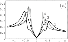
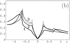
The second reason for the ratio $2\Delta_{g}/T_{p}$ to get larger is the following. As it was already mentioned above, in the inhomogeneous situation with an atomic-scale single perturbation of the large enough strength the main peak in LDOS does not represent the maximal local superconducting gap on the Fermi surface, but originates from the spectral weight transfer from the nearby van Hove singularity due to the Andreev scattering processes. For the tight-binding parameters we consider the van Hove singularity energy in the homogeneous system is approximately described by the formula $\varepsilon_{vH}=-\sqrt{(-\mu+4t^{\prime})^{2}+\Delta_{max}^{2}}$, where $\Delta_{max}$ is an effective maximal superconducting gap on the Fermi surface. The processes of Andreev scattering from the inhomogeneity result in appearing of the symmetrical with respect to Fermi energy peak in LDOS. The examples of low-temperature LDOS curves exhibiting such a feature are shown in Fig. 4. Panels (a) and (b) correspond to models (a) and (b), respectively. It is seen that for model (a), where the normal state van Hove singularity is very close to the Fermi energy (and, consequently, the van Hove singularity peak in the superconducting state is close to the superconducting coherence peak), the above mentioned transfer of the spectral weight leads to small enough increase of the gap $\Delta_{g}$. The shape of the resulting peak is close to the shape of a superconducting coherence peak because of partial overlapping of the van Hove singularity and superconducting coherence peak in the bulk. At the same time for model (b), where the van Hove singularity is more distinct from the superconducting coherence peak in the bulk, the clearly seen spectral weight transfer results in considerable increase of the gap $\Delta_{g}$. However, this mechanism of a gap enhancement is very local, as it is seen in Fig. 4(b). This is the reason for appearing of very high gap just at the plaquette occupied by the perturbation in Fig. 2(b). However, the shape of the resulting peak is strongly distorted. It is worth to note that the LDOS curves represented here are related to the single perturbation. For the many individual perturbations discussed below the curves have more resemblance to the experimentally measured LDOS spectra.

Figure 4: Low-temperature ($T=0.03$) LDOS curves taken for a number of sites from the center of the perturbation (black solid curve) to the background (gray line). The curves correspond to the sites marked by the appropriate numbers in Fig. 1(a) and Fig. 2(a). Panels (a) and (b) correspond to models (a) and (b), respectively.

II.3 many OP scatterers

Now we turn to discussion of more realistic situation, when many pair interaction scatterers are present in the sample. We have considered a $22\times 22$ sites square as a perturbation described by the T-matrix. We again represent here two models. In the both models individual perturbations are randomly distributed in the square with the concentration $n=0.07$ (here concentration means the number of individual scatterers divided by the total number of sites in the square). In model (A) the individual perturbations have the same shape as in the single perturbation model (a). Model (B) corresponds to the individual perturbations described by model (b). The tight-binding parameters describing the normal state quasiparticle dispersion coincide for models (a) and (A) so as for models (b) and (B), respectively. The numerical values of the parameters, characterizing the individual scatterers, are taken to give the same low-temperature values of superconducting OP in the center of the perturbation and in the background as for the corresponding single perturbation model (see captions to Figs. 5 and 6 for the particular values).

Since we consider the finite-size square as a perturbation described by $T$-matrix, the finite-size effects will affect the results. However the appropriate choice of the homogeneous superconducting OP $\Delta^{0}$ outside the square helps us to minimize the influence of the square boundary. By considering a larger $30\times 30$ sites square we have checked that if the bulk OP outside the square is taken to be equal to the average background value of the OP in the square, the error in calculating OP, gap and $T_{p}$ becomes less than $5\%$ at the distance $\sim 4$ sites from the boundary and lessens further towards the center of the square. For this reason the $14\times 14$ central region of the square is taken into account in calculating the statistical properties of the system.

The resulting spatial distributions of low-temperature site-averaged OP, low-temperature gap-maps and $T_{p}$ maps are demonstrated in Figs. 5 and 6 for models (A) and (B), respectively. It is worth to note that the temperature evolution of OP spatial distribution was already discussed in Ref. andersen06, , so we do not focus here on this aspect. The spatial distributions of low-temperature OP are represented in Figs. 5(a) and 6(a). As it was described earlier for the single perturbation, the spatial profile of the OP inhomogeneity mainly follows that one of the coupling constant, that is the characteristic scale of the corresponding inhomogeneity is $\sim 2$ atomic sites. However, due to discussed above fact that the deviation of the Green’s function from the bulk value is spread over a wider space region than the superconducting OP, the gap and $T_{p}$ inhomogeneities are more smooth and the characteristic size of the patches in the gap and $T_{p}$ maps is of the order of $4-5$ atomic sites for model (A) and $\sim 3$ atomic sites for model (B). For model (A) the size of a patch is roughly in accordance with the superconducting coherence length $\xi_{s}$, while for model (B) it is somewhat smaller due to very spiky character of the perturbation.

Figure 5: (a) Low-temperature ($T=0.05$) distribution of the site-averaged OP for model (A). (b) Low-temperature gap map. (c) $T_{p}-$map. (d) Histogram of $2\Delta_{g}(i)/T_{p}(i)$ values. The parameters describing a perturbation are the following: $g_{b}=0.05$, $\delta g=2.72$, $\lambda=z=1.5$.

Figure 6: (a) Low-temperature ($T=0.03$) distribution of the site-averaged OP for model (B). (b) Low-temperature gap map. (c) $T_{p}-$map. (d) Histogram of $2\Delta_{g}(i)/T_{p}(i)$ values. The individual perturbation and the background are described by the following parameters: $g_{b}=0.25$, $u_{1}=1.16$, $u_{2}=0.25$ and $z=0.5$.

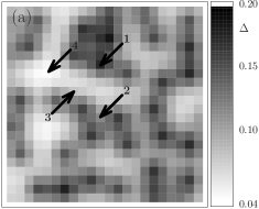
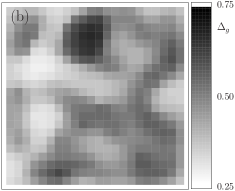
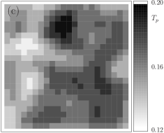
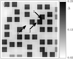
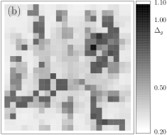
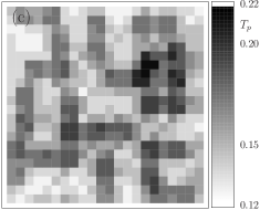
The probability distributions to find the particular value for $2\Delta_{g}(i)/T_{p}(i)$ in our model samples are plotted in Figs. 5(d) and 6(d). It is seen that the distribution for model (A) is quite narrow. The reason is that the spatial profile of the ratio $2\Delta_{g}/T_{p}$ is broadened and flattened as compared to OP spatial profile, as it was demonstrated in Fig. 1(d) and discussed in the context of the single perturbation. For model (B) the distribution is wider and exhibits a long tail of very high ratios for a small part of sites. The reason for this fact was discussed in the context of the single perturbation.

The average values of the ratio $2\Delta_{g}(i)/T_{p}(i)$ for models (A) and (B) are $5.4$ and $5.6$, respectively. These values are considerably less than the ones for the appropriate single perturbations, described by models (a) and (b) (as it was discussed earlier, for the single perturbation the ratio $\langle 2\Delta_{g}(i)/T_{p}(i)\rangle$ averaged over the region $\sim l^{2}$, where $l$ corresponds to the average distance between the centers of enhanced pairing regions for the appropriate many scatterers model, equals to $7.6$ and $8.5$ for models (a) and (b), respectively). Although the mean-field ratios for many scatterers models exceed the corresponding bulk ratios $2\Delta_{g}^{A,av}/T_{p}^{A,av}=5.2$ and $2\Delta_{g}^{B,av}/T_{p}^{B,av}=4.8$, this increase is quite small as compared to the single perturbation, especially for model (A). Here the homogeneous ratios $2\Delta_{g}^{A(B),av}/T_{p}^{A(B),av}$ are calculated for the coupling constants, which give the same zero-temperature OP, as the average zero-temperature OP in samples (A) and (B). The reason for such a crucial reduction of the ratio $2\Delta_{g}/T_{p}$ in the presence of many OP scatterers is the proximity effect. The individual perturbations essentially interact one with another for the considered concentrations when the averaged distance between them is less then the superconducting coherence length. In the framework of the mean-field treatment the phase of the OP is the same over the entire sample. For this reason the individual perturbations raise the pairing correlations in the background and maintain their own OP even for high enough temperatures in comparison with the background critical temperature. This is quite different from the picture of the single perturbation, where the pairing correlations sharply weaken for the temperatures higher than $T_{b}$.

Figure 7: The dependence of the site-averaged OP on temperature for the sites marked by the appropriate numbers in Figs. 5(a) and 6(a) (black solid lines). The gray lines are the temperature dependence of the bulk OP having the same zero-temperature value as in the center of the chosen perturbation (upper gray curve), at the chosen site belonging to the background (bottom gray curve) and as the averaged OP (middle gray curve). The dotted line represents the temperature dependence of the OP, averaged over the entire sample. Panels (a) and (b) correspond to models (A) and (B), respectively.

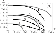
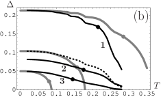
The discussed behavior of the superconducting OP is depicted in Fig. 7. Panels (a) and (b) correspond to models (A) and (B), respectively. The black solid lines represent the dependence of the site-averaged OP on temperature for the sites marked by the appropriate numbers in Figs. 5(a) and 6(a). They correspond to the characteristic OP behavior along the line from the center of the perturbation to the background (from top to bottom). The gray lines illustrate the temperature dependence of the bulk OP having the same zero-temperature value as in the center of the chosen perturbation (upper gray curve), at the chosen site belonging to the background (bottom gray curve) and as the averaged OP (middle gray curve). The dashed line represents the temperature dependence of the OP, averaged over the entire sample. Although the curves still exhibit non-BCS shape, there is no sharp suppression of the superconducting correlations in the vicinity of the background critical temperature unlike the single perturbation case. Now, roughly speaking, it is the critical temperature of the bulk OP, having the same low-temperature value as the averaged OP (middle gray curve), that plays part of the background critical temperature for the single perturbation: if the OP at a given location is less than the averaged value, the superconducting correlations for a finite temperature are higher than the bulk ones corresponding to the same zero-temperature OP, and only for the locations, where the OP exceeds the average value, the finite-temperature superconducting correlations are suppressed as compared to the bulk behavior. This leads to the fact that the values of $T_{p}(i)$ are higher than for the single perturbation case, what, in turn, results in considerable decrease of the ratio $2\Delta_{g}/T_{p}$. It is worth noting that in our mean-field treatment we neglect OP phase. However, it is physically reasonable that the phase of the superconducting order parameter should fluctuate from one region of enhanced pairing amplitude to another in such an inhomogeneous situation, as it was already mentioned in the introduction. We discuss the influence of the thermal phase fluctuations on the above results in the next section.

As it was mentioned above, the difference between the averaged ratio $\langle 2\Delta_{g}(i)/T_{p}(i)\rangle$ for model (B) and the corresponding homogeneous value is higher than between the same quantities in model (A). In addition, the probability distribution to find the particular value of the ratio has a long tail of very high values for this model. The ratio is greatly enhanced for a small part of the sites due to the fact that the mechanism of the spectral weight transfer from the van Hove singularity makes the gap considerably larger for this model, where the van Hove singularity and the bulk coherence peak are quite distinct, but it only works in the close vicinity of an individual perturbation. To illustrate this the LDOS and thermally smeared LDOS calculated according to the expression (4) at some typical sites are shown in Figs. 8(a),(b) for model (A) and Figs. 8(c),(d) for model (B), respectively. The left column represents the bare LDOS, while the right one corresponds to the thermally-smeared quantity. Please note that the temperatures we use to calculate the thermally smeared LDOS are deeply in the superconducting state, where the superconducting OP practically does not differ from its zero-temperature value.

Figure 8: LDOS (left column) and thermally smeared LDOS (right column). For all the figures the black solid curve represents LDOS at a given site typical for the background, dashed line corresponds to the center of a perturbation and LDOS somewhere between them is plotted by the dotted line. Upper row represents the results for model (A), thermally smeared LDOS is calculated at $T=0.05$. Middle row demonstrates the results for model (B), while bottom row corresponds to model (B’). Thermally smeared LDOS for models (B) and (B’) is obtained at $T=0.03$.

It is seen from the figures that for the most part of sites the bare LDOS exhibits two peaks (and also a number of kinks). The peak at smaller energies represents a superconducting coherence peak corresponding to an effective OP. This effective OP neither coincides with the background value, as it was for the single perturbation, nor represents the local OP value. Apparently, its value is close to the average over some area for the most part of the samples, however this will be discussed in more detail elsewhere bobkovy . The second peak at higher energies is usually weaker (except for the small part of sites in the sample (B)) and associated with the spectral weight transfer from the van Hove singularity due to Andreev scattering. For the both models the spectral weight transfer is clearly seen in the bare LDOS, however the two peaks overlap for model (A) due to the fact that the normal state van Hove singularity is quite close to the Fermi surface in this case. As a result the effective superconducting coherence peak and the one transferred from the van Hove singularity merge in the thermally smeared LDOS even for a low temperature, as it is seen in Fig.8(b). The resulting peak resembles a superconducting coherence peak.

For model (B) the effective superconducting coherence peak and the peak transferred from van Hove singularity are more distinct. In this case the effective coherence peak is higher than the transferred one for a number of sites. However, they are of the same order for the most part of sites. As a result the gap position is located somewhere between them in the low-temperature thermally smeared LDOS. The corresponding curves do not exhibit a pronounced peak and resemble the $dI/dV$ behavior observed in underdoped samples in contrast to model (A) LDOS, which is more similar to optimally and overdoped samples. Finally, the transferred peak wins for a small number of sites, typically at centers of the individual perturbations. This leads to the sharp increase of the gap for these spatial locations and, consequently, to the existence of the long tails in the $2\Delta_{g}/T_{p}$ distribution.

II.4 effect of weak potential and hopping element inhomogeneities

It is reasonable to assume that the possible causes of the pairing interaction inhomogeneities (for example, dopant atoms) most probably also give rise to a disorder of the normal state parameters. Therefore, let us turn to the discussion of the additional effect of inhomogeneities of tight binding parameters such as chemical potential and hopping matrix elements on the measured by STM properties. Here we only focus on a weak inhomogeneity of the chemical potential $|\delta\mu|\lesssim t$. Strong potential scatterers characterizing by $|\delta\mu|\gg t$ are well-known to give rise to quasiparticle resonant bound states in the close vicinity of the potential impurity balatsky04 . In real BSCCO system only very small part of in plane native defects exhibits near zero bias resonances, so they should not influence considerably the statistical properties studied here, such as the $2\Delta_{g}/T_{p}$ distribution.

To illustrate the influence of this additional disorder we have chosen our model (B), where the nearest neighbor hopping element is taken to be $t+\delta t$, the next-nearest neighbor equals to $t^{\prime}+\delta t^{\prime}$ and the chemical potential is $\mu+\delta\mu$ for the plaquettes corresponding to the enhanced pairing interaction. Here we take $\delta t=0.50$, $\delta t^{\prime}=0.15$ and $\delta\mu=-0.25$. This model is referred to as (B’).

The LDOS and low-temperature thermally smeared LDOS for model (B’) are shown in Figs. 8(e) and (f), respectively. As it is seen in the figures the low-energy part of the curves is practically not affected by the potential and hopping matrix element disorder. Only the high energy part and, especially the region of the van Hove singularity is distorted by this type of scatterers. The van Hove singularity become less pronounced under the influence of the additional disorder: more widened and reduced in height. This is natural because in the homogeneous situation the change of tight binding parameters strongly shifts the energy location of the van Hove singularity. It is worth to note that for the models, where the normal state van Hove singularity is more close to the Fermi energy (similar to model (A) we consider), the effect of the diagonal scatterers on the LDOS is even weaker, because the van Hove singularity is absorbed by the superconducting coherence peak and the resulting peak is not qualitatively sensitive to the discussed types of disorder, as it was shown in Ref. nunner05, for the case of weak potential disorder.

To investigate the influence of the discussed additional disorder on the properties of interest here we compare the OP, gap and $T_{p}$ spatial distributions for models (B) and (B’). The correlation between the OP spatial distributions in models (B) and (B’) is demonstrated in Fig. 9(a). The horizontal axis represents the value of the superconducting OP in model (B), while the vertical axis corresponds to this value for model (B’). Each point with the coordinates $(\Delta^{(B)},\Delta^{(B^{\prime})})$ represents the values of the superconducting OP for a given site $i$ in models (B) and (B’). The line is the linear fit $\Delta^{(B^{\prime})}=1.01\Delta^{(B)}$ to these points. It is seen that the points are described by this fit very well, so the additional disorder practically does not affect the superconducting OP.

Figure 9: (a) The correlation between the OP spatial distributions in models (B) and (B’). Each point with the coordinates $(\Delta^{(B)},\Delta^{(B^{\prime})})$ represents the values of the superconducting OP for a given site $i$ in models (B) and (B’). The line is the linear fit $\Delta^{(B^{\prime})}=1.01\Delta^{(B)}$ to these points. (b) Analogous correlation between the low-temperature ($T=0.03$) gaps in the considered models. The points are fitted by the liner dependence $\Delta_{g}^{(B^{\prime})}=0.69\Delta_{g}^{(B)}+0.18$. (c) The correlation between $T_{p}$. The linear fit is $T_{p}^{(B^{\prime})}=1.42T_{p}^{(B)}-0.06$. (d) The histograms for $2\Delta_{g}/T_{p}$ distributions. The upper histogram corresponds to model (B’), while the bottom is related to model (B). The offset is for clarity.

At the same time the gap and $T_{p}$ distributions are influenced by the potential and hopping scatterers, as it is seen in Figs. 9(b) and (c), respectively. The reason is that the gap is (at least partially) determined by the LDOS peak originated from the spectral weight transfer from the van Hove singularity by Andreev scattering processes, while, as it was discussed above, the van Hove singularity is affected quite strongly by the potential and hopping disorder. Nevertheless, the correlations between the low-temperature gaps and $T_{p}$ in models (B) and (B’) can be still fitted by a linear dependence, what indicates the fact that the corresponding gap maps do not change qualitatively under the influence of such a disorder, but only distorted to a certain extent. The average values of the low-temperature gap and $T_{p}$ also differ very slightly for models (B) and (B’): $\langle\Delta_{g}^{(B^{\prime})}\rangle=0.50$ and $\langle T_{p}^{(B^{\prime})}\rangle=0.17$, while $\langle\Delta_{g}^{(B)}\rangle=0.47$ and $\langle T_{p}^{(B)}\rangle=0.16$.

The distributions of the ratio $2\Delta_{g}/T_{p}$ for models (B) and (B’) are compared in Fig. 9(d). The average value of the ratio is again affected by the potential and hopping disorder only slightly: $\langle 2\Delta_{g}/T_{p}\rangle=5.8$ for model (B’) and $\langle 2\Delta_{g}/T_{p}\rangle=5.6$ for model (B), although the disorder results in widening of the distribution.

At the end of the discussion of the potential and hopping disorder effect we would like to note that the considered here set of parameters is just a representative example. We have studied a number of other weak potential and hopping disorder configurations and found that their effect qualitatively the same. Although the particular values for the potential and hopping disorder parameters and their relationship to the pair disorder strength can be only established in the framework of certain microscopic models, our analysis indicates that they do not qualitatively influence the physics discussed in the present paper.

III Thermal phase fluctuations: a toy model

The considered above mean-field approximation seems to be physically not quite appropriate for studying the state, which is inhomogeneous on the atomic scale, especially in view of short coherence length in cuprate materials. It is reasonable to assume that the phase of the superconducting order parameter should fluctuate from one region of enhanced pairing amplitude to another in such an inhomogeneous situation, what can significantly suppress the temperature $T_{p}$ and, consequently, increase the ratio $2\Delta/T_{p}$. The regular consideration of the state with inhomogeneous pairing interaction beyond the framework of mean-field approximation, which takes into account thermal phase fluctuations, is a separate problem. So we postpone it for a future publication. To show that the thermal phase fluctuations are indeed systematically suppress $T_{p}$, in the present paper we study their effect in the framework of a toy model.

While in the mean-field approximation the phase of the superconducting OP is the same over the entire sample, we assume that it only remains constant over the region $\sim l^{2}$ around an individual perturbation, where $l$ is an average distance between the perturbations. The value of the phase in the vicinity of a perturbation centered at a site $i$ for a given temperature $T$ is set by hand according to the formula $\gamma T\{\Theta_{i}\}$, where $\{\Theta_{i}\}$ is a random number belonging to the interval $[-\pi/2,\pi/2]$ and $\gamma$ is a coefficient accounting for the strength of the fluctuations. As it is seen from the above expression the phases at different perturbation regions are partially correlated for low enough temperatures and the variation rises with temperature modelling the effect of the thermal fluctuations. The particular law of increasing the fluctuations with rising temperature (linear in the considered model) is not very important. Anyway, the main effect of the thermal phase fluctuations is to suppress $T_{p}$ considerably. The reason for this is that they partially destroy the proximity effect between different perturbation regions thus shifting the physical properties in the vicinity of a given pair scatterer to the limit of an independent single perturbation.

To demonstrate the discussed above effect in the framework of our toy model, in Figs. 10(a) and 11(a) we plotted the part of the sample gapped at a given temperature as a function of temperature for models (A) and (B), respectively. The black solid line in Fig. 10(a) [11(a)] represents the results for the pure mean-field model (A) [(B)] without phase fluctuations, the dashed lines demonstrate the effect of weak enough fluctuations corresponding to $\gamma=5$ and the dotted lines are related to more stronger fluctuations with $\gamma=10$. It is seen that the increase in the fluctuation strength $\gamma$ monotonously suppresses $T_{p}$.

Figure 10: (a) The part of the sample gapped at a given temperature as a function of temperature. The black solid line corresponds to the mean-field results, the dashed line demonstrates the effect of weak enough fluctuations described by $\gamma=5$ and the dotted line is related to more stronger fluctuations with $\gamma=10$. (b) The influence of the fluctuations on the $2\Delta_{g}(i)/T_{p}(i)$ distribution. The bottom histogram is calculated for the mean-field sample, while the middle one is for the weaker fluctuations with $\gamma=5$ and the upper distribution corresponds to $\gamma=10$. All the results are related to model (A).

Figure 11: The same results as in Fig. 10, but calculated for model (B).

Figs. 10(b) and 11(b) represent the influence of the fluctuations on the $2\Delta_{g}/T_{p}$ distributions for models (A) and (B), respectively. The bottom histograms correspond to the mean-field samples, while the middle ones are related to the weaker fluctuations with $\gamma=5$ and the upper distributions are calculated for the more stronger fluctuations modelling by $\gamma=10$. It is clearly seen for the both models that the increase of the phase variation monotonously shifts the distribution to more higher values without considerable changing of its shape. The average values of the ratio $2\Delta_{g}/T_{p}$ corresponding to all the histograms are represented in the Table 1. It is worth to note that the average ratios corresponding to the stronger fluctuations with $\gamma=10$ (last column in Tab. 1) are in excellent agreement with the appropriate ratios for the single perturbations. This points to the fact that these fluctuations suppress the proximity effect between neighbor enhanced pairing regions quite efficiently, so that the limit of single perturbation is practically reached for an individual perturbation region.

$\gamma$	0	5	10
(A)	5.4	6.5	7.6
(B)	5.6	6.9	8.6

Table 1: The values of the ratio $\langle 2\Delta_{g}/T_{p}\rangle$ for all the histograms shown in Figs. 10(b) and 11(b). The first column corresponds to the mean-field results, while the second and third ones represent their shift under the influence of weak and strong fluctuations, respectively. The middle row is related to model (A), and correspondingly to Fig. 10(b). The bottom one contains the average ratios for model (B) and, consequently, for the histograms in Fig. 11(b).

The results demonstrated in Figs. 10, 11 and Tab. 1 are calculated for a given random realization of the parameters $\{\Theta_{i}\}$. Having studied a number of random realizations of these parameters we found that the absolute error in determining the average ratio $\langle 2\Delta_{g}/T_{p}\rangle$ is $\sim 0.2$.

IV Anticorrelation between low-temperature gap and high-temperature zero-bias conductance

As it was shown above, one of the characteristic features of the model with the atomic-scale inhomogeneity of the superconducting OP is the considerable enhancement of the ratio $2\Delta_{g}/T_{p}$ as compared to the homogeneous case. In this section we would like to discuss another characteristic manifestation of the OP inhomogeneity in the spectra measured by STM. It was recently reportedyazdani08 that the value of the low-temperature position-dependent gap obtained from the STM spectra strongly anticorrelated with the value of zero-bias differential conductance at a temperature, where practically the entire sample is ungapped. One of possible explanations for this experimental observation can be naturally given in the framework of the inhomogeneous OP model.

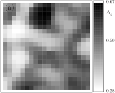
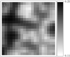
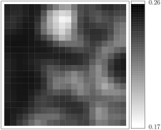
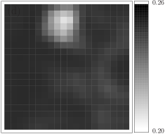
Fig. 12 demonstrates the low-temperature gap-map (panel (a)) in comparison with the maps of high-temperature zero-bias thermally smeared LDOS (panels (b)-(d)). All the maps correspond to the considered above model (A) in the mean-field approximation. High-temperature zero-bias thermally smeared LDOS is calculated according to the formula (4) at V=0 for three different temperatures: the results for $T=0.15$, where $80\%$ of the sample are still gapped, are shown in panel (b), while panel (c) is related to $T=0.19$, where only $2\%$ of the sample are gapped and panel (d) corresponds to $T=0.21$, where the entire sample is already ungapped. The anticorrelation between the maps in panel (a) from one hand and the maps in panels (b)-(d) is clearly seen. Fig. 13(a) further quantifies this anticorrelation. High-temperature zero-bias thermally smeared LDOS, measured along the vertical axis, versus low-temperature gap (horizontal axis) is plotted in this figure for all the sites of our sample.

Figure 12: (a) The low-temperature ($T=0.05$) gap map for model (A). (b)-(d) The zero-bias space distributions of the thermally-smeared LDOS for the same model: (b) $T=0.15$, (c) $T=0.19$ and (d) $T=0.21$.

As it was described above in detail, the atomic-scale OP inhomogeneity leads to the fact, that the difference between the temperature of vanishing the gap $T_{p}(i)$ and the temperature of disappearing the pair correlations, which corresponds to the critical temperature $T_{x}$ in the mean-field treatment, is considerably higher for the inhomogeneous situation as compared to the homogeneous case. The temperature evolution of thermally smeared LDOS from $T=0.15$ to $T=0.21$ is demonstrated in Figs. 13(b)-(d) for three typical space locations. Only very small part of the sample exhibits the behavior shown in panel (b), while approximately $2/3$ of the sample can be described by panel (c) and the behavior of the conductance for the last $1/3$ of the sites corresponds to panel (d).

Figure 13: (a) High-temperature zero-bias thermally-smeared LDOS, measured along the vertical axis, versus low-temperature gap (horizontal axis) for all the sites of the sample at three different temperatures: $T=0.15$, $T=0.19$ and $T=0.21$. (b)-(d) The temperature evolution of thermally smeared LDOS for three typical spatial locations. $T=0.15$ (solid black lines), $T=0.19$ (dashed lines) and $T=0.21$ (dotted lines). All the panels are related to model (A).

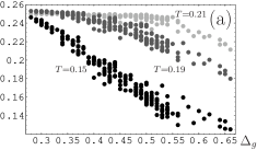
That is, although practically the entire sample is ungapped at $T=0.19$ for our model (A) and the conductance curves change only slightly or practically do not change under further increasing in the temperature, the value of the superconducting OP is not small for the most part of the sample at this temperature (see Fig. 7(a)). Even the complete vanishing of the gap at $T=0.21$ does not mean that there are no pair correlations in the system. The presence and the strength of the pair correlations is reflected in the suppression of the low-energy LDOS. It is clearly seen in Figs. 12(a)-(d) and 13(a) that the anticorrelation weakens with temperature. It is rather weak at $T=0.21$, where the pair correlations are small, and should disappear in the framework of our model when the pair correlations entirely vanish. We believe that this scenario should also work if one takes into account the thermal phase fluctuations because the same physical picture is valid for the single perturbation as well. However, a regular theory is needed for a detailed consideration of this problem.

V Conclusions

We have studied the influence of the atomic-scale inhomogeneities of the superconducting OP on the conductance spectra measured by STM. First of all, it is found that the ratio of the local low-temperature gap in differential conductance spectra to the local temperature of vanishing the gap $2\Delta_{g}/T_{p}$ can take large enough values as compared to the homogeneous OP model. While in the framework of the mean-field approximation the ratio does not strongly differ from the homogeneous one, the thermal phase fluctuations considerably enhance it. At least in the framework of a very simplified model we obtained that the ratio $2\Delta_{g}/T_{p}$ can reach the values $\sim 7-8$, which are comparable to the experimental ones. It is also demonstrated that the additional weak potential scatterers and hopping matrix element disorder do not influence qualitatively the above results. Second, the atomic-scale OP inhomogeneity results in the anticorrelation between the low-temperature gap and the high-temperature zero-bias conductance, bearing a resemblance to the recent results obtained by STM.

VI Acknowledgments

The support by the Russian Science Support Foundation (A.M.B.), RF Presidential Grant No.MK-4605.2007.2 (I.V.B.) and the programs of Physical Science Division of RAS are acknowledged.

References

- (1) T. Cren, D. Roditchev, W. Sacks, J. Klein, J.-B. Moussy, C. Deville-Cavellin, and M. Laguës, Phys. Rev. Lett. 84, 147 (2000).
- (2) S.H. Pan, J.P. O’Neal, R.L. Badzey, C. Chamon, H. Ding, J.R. Engelbrecht, Z. Wang, H. Eisaki, S. Uchida, A.K. Gupta, K.-W. Ng, E.W. Hudson, K.M. Lang, and J.C. Davis, Nature (London) 413, 282 (2001).
- (3) C. Howard, P. Fournier, and A. Kapitulnik, Phys. Rev. B 64, 100504 (2001).
- (4) K.M. Lang, V. Madhavan, J.E. Hoffman, E.W. Hudson, H. Eisaki, S. Uchida, and J.C. Davis, Nature (London) 415, 412 (2002).
- (5) K. McElroy, J. Lee, J.A. Slezak, D.H. Lee, H. Eisaki et al., Science 309, 1048 (2005).
- (6) A.C. Fang, L. Capriotti, D.J. Scalapino, S.A. Kivelson, N. Kaneko, M. Greven, and A. Kapitulnik, Phys. Rev. Lett. 96, 017007 (2006).
- (7) T. Kato, T. Maruyama, S. Okitsu, and H. Sakata, arxiv:0803.1415 (unpublished).
- (8) I. Martin and A.V. Balatsky, Physica C 357, 46 (2001).
- (9) Z. Wang, J.R. Engelbrecht, S. Wang, H. Ding, and S.H. Pan, Phys. Rev. B, 65, 064509 (2002).
- (10) Q.-H. Wang, J.H. Han, and D.-H. Lee, Phys. Rev. B, 65, 054501 (2002).
- (11) S. Zhou, H. Ding, and Z. Wang, Phys. Rev. Lett., 98, 076401 (2007).
- (12) S.A. Kivelson, I.P. Bindloss, E. Fradkin, V. Oganesyan, J.M. Tranquada, A. Kapitulnik, and C. Howald, Rev. Mod. Phys. 75, 1201 (2003).
- (13) W.A. Atkinson, Phys. Rev. B, 71, 024516, (2005).
- (14) G. Alvarez, M. Mayr, A. Moreo, and E. Dagotto, Phys. Rev. B 71, 014514 (2005).
- (15) A. Ghosal, A. Kopp, and S. Chakravarty, Phys. Rev. B 72, 220502(R) (2005).
- (16) D. Podolsky, E. Demler, K. Damle, and B.I. Halperin, Phys. Rev. B 67, 094514 (2003).
- (17) H.-D. Chen, O. Vafek, A. Yazdani, S.-C. Zhang, Phys. Rev. Lett. 93, 187002 (2004).
- (18) T. Nunner, B.M. Andersen, A. Melikyan, and P.J. Hirschfeld, Phys. Rev. Lett. 95, 177003 (2005).
- (19) T. Timusk and B. Statt, Rep. Prog. Phys. 62, 61 (1999).
- (20) M.R. Norman, D. Pines, and C. Kallin, Adv. Phys. 54, 715 (2005).
- (21) P.A. Lee, N. Nagaosa, and X.-G. Wen, Rev. Mod. Phys. 78, 17 (2006).
- (22) A.J. Millis, Science 314, 1888 (2006).
- (23) A. Cho, Science 314, 1072 (2006).
- (24) K.K. Gomes, A.N. Pasupathy, A. Pushp, S. Ono, Y. Ando, and A. Yazdani, Nature(London), 447, 569 (2007).
- (25) A.N. Pasupathy, A. Pushp, K.K. Gomes, C.V. Parker, J. Wen, Z. Xu, G. Gu, S. Ono, Y. Ando, and A. Yazdani, Science, 320, 196 (2008).
- (26) P. Monthoux and D.J. Scalapino, Phys. Rev. Lett. 72, 1874 (1994).
- (27) K. Aryanpour, E.R. Dagotto, M. Mayr, T. Paiva, W.E. Pickett, and R.T. Scalettar, Phys. Rev. B 73, 104518 (2006); K. Aryanpour, T. Paiva, W.E. Pickett, and R.T. Scalettar, Phys. Rev. B 76, 184521 (2007).
- (28) Y. Zou, I. Klich, and G. Refael, Phys. Rev. B 77, 144523 (2008).
- (29) M. Franz, C. Kallin, A.J. Berlinsky, and M.I. Salkola, Phys. Rev. B 56, 7882 (1997).
- (30) G. Alvarez and E. Dagotto, arxiv:0802.3394 (unpublished).
- (31) M. R. Norman, H. Ding, M. Randeria, J. C. Campuzano, T. Yokoya, T. Takeuchi, T. Takahashi, T. Mochiku, K. Kadowaki, P. Guptasarma, D. G. Hinks, Nature 392, 157 (1998).
- (32) A. Kanigel, M. R. Norman, M. Randeria, U. Chatterjee, S. Suoma, A. Kaminski, H. M. Fretwell, S. Rosenkranz, M. Shi, T. Sato, T. Takahashi, Z. Z. Li, H. Raffy, K. Kadowaki, D. Hinks, L. Ozyuzer, J. C. Campuzano, Nature Physics 2, 447 (2006).
- (33) A. Kanigel, U. Chatterjee, M. Randeria, M. R. Norman, S. Souma, M. Shi, Z. Z. Li, H. Raffy, J. C. Campuzano, Phys. Rev. Lett. 99, 157001 (2007).
- (34) Y. Dubi, Y. Meir, and Y. Avishai, Nature 449, 876 (2007).
- (35) Yu.N. Ovchinnikov, S.A. Wolf, and V.Z. Kresin, Phys. Rev. B 63, 064524 (2001).
- (36) B.M. Andersen, A. Melikyan, T.S. Nunner, and P.J. Hirschfeld, Phys. Rev. B 74, 060501 (2006).
- (37) I.V. Bobkova and A.M. Bobkov, in preparation.
- (38) A.V. Balatsky, I. Vekhter, and J.-X. Zhu, Rev. Mod. Phys. 78, 373 (2006).