Explicit expressions for moments of the beta Weibull distribution

Abstract

The beta Weibull distribution was introduced by Famoye et al. (2005) and studied by these authors. However, they do not give explicit expressions for the moments. We now derive explicit closed form expressions for the cumulative distribution function and for the moments of this distribution. We also give an asymptotic expansion for the moment generating function. Further, we discuss maximum likelihood estimation and provide formulae for the elements of the Fisher information matrix. We also demonstrate the usefulness of this distribution on a real data set.
Keywords: Beta Weibull distribution, Fisher information matrix, Maximum likelihood, Moment, Weibull distribution.

1 Introduction

The Weibull distribution is a popular distribution widely used for analyzing lifetime data. We work with the beta Weibull (BW) distribution because of the wide applicability of the Weibull distribution and the fact that it extends some recent developed distributions. This generalization may attract wider application in reliability and biology. We derive explicit closed form expressions for the distribution function and for the moments of the BW distribution. An application is illustrated to a real data set with the hope that it will attract more applications in reliability and biology, as well as in other areas of research.

The BW distribution stems from the following general class: if $G$ denotes the cumulative distribution function (cdf) of a random variable then a generalized class of distributions can be defined by

$$F(x)=I_{G(x)}(a,b)$$ (1)

for $a>0$ and $b>0$, where

$$I_{y}(a,b)=\frac{B_{y}(a,b)}{B(a,b)}=\frac{\int_{0}^{y}w^{a-1}(1-w)^{b-1}dw}{B(a,b)}$$

is the incomplete beta function ratio, $B_{y}(a,b)$ is the incomplete beta function, $B(a,b)=\Gamma(a)\Gamma(b)/\Gamma(a+b)$ is the beta function and $\Gamma(.)$ is the gamma function. This class of generalized distributions has been receiving increased attention over the last years, in particular after the recent works of Eugene et al. (2002) and Jones (2004). Eugene et al. (2002) introduced what is known as the beta normal distribution by taking $G(x)$ in (1) to be the cdf of the normal distribution with parameters $\mu$ and $\sigma$. The only properties of the beta normal distribution known are some first moments derived by Eugene et al. (2002) and some more general moment expressions derived by Gupta and Nadarajah (2004). More recently, Nadarajah and Kotz (2004) were able to provide closed form expressions for the moments, the asymptotic distribution of the extreme order statistics and the estimation procedure for the beta Gumbel distribution. Another distribution that happens to belong to (1) is the log$\,F$ (or beta logistic) distribution, which has been around for over 20 years (Brown et al., 2002), even if it did not originate directly from (1).

While the transformation (1) is not analytically tractable in the general case, the formulae related with the BW turn out manageable (as it is shown in the rest of this paper), and with the use of modern computer resources with analytic and numerical capabilities, may turn into adequate tools comprising the arsenal of applied statisticians. The current work represents an advance in the direction traced by Nadarajah and Kotz (2006), contrary to their belief that some mathematical properties of the BW distribution are not tractable.

Thus, following (1) and replacing $G(x)$ by the cdf of a Weibull distribution with parameters $c$ and $\lambda$, we obtain the cdf of the BW distribution

$$F(x)=I_{1-{\rm exp}\{-(\lambda x)^{c}\}}(a,b)$$ (2)

for $x>0$, $a>0$, $b>0$, $c>0$ and $\lambda>0$. The corresponding probability density function (pdf) and the hazard rate function associated with (2) are:

$$f(x)=\frac{c\lambda^{c}}{B(a,b)}x^{c-1}{\rm exp}\{-b(\lambda x)^{c}\}[1-{\rm exp}\{-(\lambda x)^{c}\}]^{a-1},$$ (3)

and

$$\tau(x)=\frac{c\lambda^{c}x^{c-1}{\rm exp}\{-b(\lambda x)^{c}\}[1-{\rm exp}\{-(\lambda x)^{c}\}]^{a-1}}{B_{1-{\rm exp}\{-(\lambda x)^{c}\}}(a,b)},$$ (4)

respectively. Simulation from (3) is easy: if $B$ is a random number following a beta distribution with parameters $a$ and $b$ then $X=\{-{\rm log}(1-B)\}^{1/c}/\lambda$ will follow a BW distribution with parameters $a,b,c$ and $\lambda$. Some mathematical properties of the BW distribution are given by Famoye et al. (2005) and Lee et al. (2006).

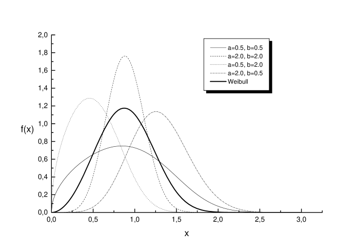
Graphical representation of equations (3) and (4) for some choices of parameters $a$ and $b$, for fixed $c=3$ and $\lambda=1$, are given in Figures 1 and 2, respectively. It should be noted that a single Weibull distribution for the particular choice of the parameters $c$ and $\lambda$ is here generalized by a family of curves with a variety of shapes, shown in these figures.

The rest of the paper is organized as follows. In Section 2, we obtain some expansions for the cdf of the BW distribution, and point out some special cases that have been considered in the literature. In Section 3, we derive explicit closed form expressions for the moments and present skewness and kurtosis for different parameter values. Section 4 gives an expansion for its moment generating function. In Section 5, we discuss the maximum likelihood estimation and provide the elements of the Fisher information matrix. In Section 6, an application to real data is presented, and finally, in Section 7, we provide some conclusions. In the appendix, two identities needed in Section 3 are derived.

Figure 1: The probability density function (3) of the BW distribution, for several values of parameters $a$ and $b$

Figure 2: The hazard function (4) of the BW distribution, for several values of parameters $a$ and $b$

2 Expansions for the distribution function

The BW distribution is an extended model to analyze more complex data and generalizes some recent developed distributions. In particular, the BW distribution contains the exponentiated Weibull distribution (for instance, see Mudholkar et al., 1995, Mudholkar and Hutson, 1996, Nassar and Eissa, 2003, Nadarajah and Gupta, 2005 and Choudhury, 2005) as special cases when $b=1$. The Weibull distribution (with parameters $c$ and $\lambda$) is clearly a special case for $a=b=1$. When $a=1$, (3) follows a Weibull distribution with parameters $\lambda\,b^{1/c}$ and $c$. The beta exponential distribution (Nadarajah and Kotz, 2006) is also a special case for $c=1$.

In what follows, we provide two simple formulae for the cdf (2), depending on whether the parameter $a>0$ is real non-integer or integer, which may be used for further analytical or numerical analysis. Starting from the explicit expression for the cdf (2)

$$F(x)=\frac{c\lambda^{c}}{B(a,b)}\int_{0}^{x}y^{c-1}\exp\{-b(\lambda y)^{c}\}[1-\exp\{-(\lambda y)^{c}\}]^{a-1}dy,$$

the change of variables $(\lambda y)^{c}=u$ yields

$$F(x)=\frac{1}{B(a,b)}\int_{0}^{(\lambda x)^{c}}e^{-bu}(1-e^{-u})^{a-1}du.$$

If $a>0$ is real non-integer we have

$$(1-z)^{a-1}=\sum_{j=0}^{\infty}\frac{(-1)^{j}\Gamma(a)z^{j}}{\Gamma(a-j)j!}.$$ (5)

It follows that

$$F(x) = \frac{1}{B(a,b)}\int_{0}^{(\lambda x)^{c}}e^{-bu}\sum_{j=0}^{\infty}\frac{(-1)^{j}\Gamma(a)e^{-ju}}{\Gamma(a-j)j!}du$$

$$= \frac{1}{B(a,b)}\sum_{j=0}^{\infty}\frac{(-1)^{j}\Gamma(a)}{\Gamma(a-j)j!}\int_{0}^{(\lambda x)^{c}}e^{-(b+j)u}du$$

$$= \frac{1}{B(a,b)}\sum_{j=0}^{\infty}\frac{(-1)^{j}\Gamma(a)}{\Gamma(a-j)j!(b+j)}\{1-e^{-(b+j)(\lambda x)^{c}}\}.$$

Finally, we obtain

$$F(x)=\frac{\Gamma(a+b)}{\Gamma(b)}\sum_{j=0}^{\infty}\frac{(-1)^{j}\{1-e^{-(b+j)(\lambda x)^{c}}\}}{\Gamma(a-j)j!(b+j)}.$$ (6)

For positive real non-integer $a$, the expansion (6) may be used for further analytical and/or numerical studies. For integer $a$ we only need to change the formula used in (5) to the binomial expansion to give

$$F(x)=\frac{1}{B(a,b)}\sum_{j=0}^{a-1}\binom{a-1}{j}\frac{(-1)^{j}\{1-e^{-(b+j)(\lambda x)^{c}}\}}{(b+j)}.$$ (7)

When both $a$ and $b=n-a+1$ are integers, the relation of the incomplete beta function to the binomial expansion gives

$$F(x)=\sum_{j=a}^{n}\binom{n}{j}[1-{\rm exp}\{-(\lambda x)^{c}\}]^{j}{\rm exp}\{-(n-j)(\lambda x)^{c}\}.$$ (8)

It can be found in the Wolfram Functions Site that for integer $a$

$$I_{y}(a,b)=1-\frac{(1-y)^{b}}{\Gamma(b)}\sum_{j=0}^{a-1}\frac{\Gamma(b+j)y^{j}}{j!},$$

and for integer $b$,

$$I_{y}(a,b)=\frac{y^{a}}{\Gamma(a)}\sum_{j=0}^{b-1}\frac{\Gamma(a+j)(1-y)^{j}}{j!}.$$

Then, if $a$ is integer, we have another equivalent form for (7)

$$F(x)=1-\frac{{\rm exp}\{-b(\lambda x)^{c}\}}{\Gamma(b)}\sum_{j=0}^{a-1}\frac{\Gamma(b+j)}{j!}[1-{\rm exp}\{-(\lambda x)^{c}\}]^{j}.$$ (9)

For integer values of $b$, we have

$$F(x)=\frac{[1-{\rm exp}\{-(\lambda x)^{c}\}]^{a}}{\Gamma(a)}\sum_{j=0}^{b-1}\frac{\Gamma(a+j)}{j!}{\rm exp}\{-j(\lambda x)^{c}\}.$$ (10)

Finally, if $a=1/2$ and $b=1/2$, we have

$$F(x)=\frac{2}{\pi}{\rm arctan}\sqrt{{\rm exp}\{(\lambda x)^{c}\}-1}.$$ (11)

The particular cases (9) and (10) were discussed generally by Jones (2004), and the expansions (6)-(11) reduce to Nadarajah and Kotz’s (2006) results for the beta exponential distribution by setting $c=1$. Clearly, the expansions for the BW density function are obtained from (6) and (7) by simple differentiation. Hence, the BW density function can be expressed in a mixture form of Weibull density functions.

3 Moments

Let $X$ be a BW random variable following the density function (3). We now derive explicit expressions for the moments of $X$. We now introduce the following notation (for any real $d$ and $a$ and $b$ positive)

$$S_{d,b,a}=\int_{0}^{\infty}x^{d-1}{\rm exp}(-bx)\{1-{\rm exp}(-x)\}^{a-1}dx.$$ (12)

The change of variables $x=-{\rm log}(z)$ immediately yields $S_{1,b,a}=B(a,b)$. On the other hand, the change of variables $x=(\lambda y)^{c}$ gives the following relation

$$\int_{0}^{\infty}y^{\gamma-1}{\rm exp}\{-b(\lambda y)^{c}\}[1-{\rm exp}\{-(\lambda y)^{c}\}]^{a-1}dy=\frac{\lambda^{-\gamma}}{c}S_{\frac{\gamma}{c},b,a},$$ (13)

from which it follows that

$$S_{\gamma/c,b,a}=B(a,b)\lambda^{\gamma-c}E(X^{\gamma-c}),$$

or, equivalently, for any real $r$

$$E(X^{r})=\frac{1}{\lambda^{r}B(a,b)}S_{r/c+1,b,a},$$ (14)

relating $S_{r/c+1,b,a}$ to the $r$th generalized moment of the beta Weibull.

First, we consider the integral (12) when $d$ is an integer. Let $U$ be a random variable following the Beta$(b,a)$ distribution with pdf $f_{U}(\cdot)$ and $W=-{\rm log}(U)$. Further, let $F_{U}(\cdot)$ and $F_{W}(\cdot)$ be the cdf’s of $U$ and $W$, respectively. It is easy to see that $F_{W}(x)=1-F_{U}(e^{-x})$. Further, by the properties of the Lebesgue-Stiltjes integral, we have

$$E(W^{d-1}) = \int_{-\infty}^{\infty}x^{d-1}dF_{W}(x)=\int_{0}^{\infty}x^{d-1}e^{-x}f_{U}(e^{-x})dx$$

$$= \frac{1}{B(a,b)}\int_{0}^{\infty}x^{d-1}e^{-bx}(1-e^{-x})^{a-1}dx$$

$$= \frac{S_{d,b,a}}{B(a,b)}.$$

Thus, the values of $S_{d,b,a}$ for integer values of $d$ can be found from the moments of $W$ if they are known. However, the moment generating function (mgf) $M_{W}(t)=E(e^{tW})$ of $W$ can be expressed as

$$M_{W}(t) = E(U^{-t})=\frac{1}{B(a,b)}\int_{0}^{1}x^{b-t-1}(1-x)^{a-1}dx$$

$$= \frac{B(b-t,a)}{B(a,b)}.$$

This formula is well defined for $t<b$. However, we are only interested in the limit $t\rightarrow 0$ and therefore this expression can be used for the current purpose. We can write

$$S_{d,b,a}=B(a,b)E(W^{d-1})=B(a,b)M_{W}^{(d-1)}(0)=\left.\frac{\partial^{d-1}}{\partial t^{d-1}}B(b-t,a)\right|_{t=0}.$$ (15)

From equations (14) and (15) for any positive integer $k$ we obtain a general formula

$$E(X^{kc})=\frac{1}{\lambda^{kc}B(a,b)}\left.\frac{\partial^{k}}{\partial t^{k}}B(b-t,a)\right|_{t=0}.$$ (16)

As particular cases, we can see directly from (15) that

$$S_{1,b,a}=B(a,b),S_{2,b,a}={B(a,b)\left\{\psi\left(a+b\right)-\psi\left(b\right)\right\}}$$

and

$$S_{3,b,a}=B\left(a,b\right)[\psi^{\prime}\left(b\right)-\psi^{\prime}\left(a+b\right)+\left\{\psi\left(a+b\right)-\psi\left(b\right)\right\}^{2}],$$

and by using (14) we find

$$E(X^{c})=\frac{\left\{\psi\left(a+b\right)-\psi\left(b\right)\right\}}{\lambda^{c}}$$

and

$$E(X^{2c})=\frac{\psi^{\prime}\left(b\right)-\psi^{\prime}\left(a+b\right)+\left\{\psi\left(a+b\right)-\psi\left(b\right)\right\}^{2}}{\lambda^{2c}}.$$

The same results can also be obtained directly from (16).

Note that the formula for $S_{1,b,a}$ matches the one just given after equation (12). Since the BW distribution for $c=1$ reduces to the beta exponential distribution, the above formulae for $E(X^{c})$ and $E(X^{2c})$ reduce to the corresponding ones obtained by Nadarajah and Kotz (2006).

Our main goal here is to give the $r$th moment of $X$ for every positive integer $r$. In fact, in what follows we obtain the $r$th generalized moment for every real $r$ which may be used for further theoretical or numerical analysis. To this end, we need to obtain a formula for $S_{d,b,a}$ that holds for every positive real $d$. In the appendix we show that for any $d>0$ the following identity holds for positive real non-integer $a$

$$S_{d,b,a}=\Gamma(a)\Gamma\left(d\right)\sum_{j=0}^{\infty}\frac{(-1)^{j}}{\Gamma(a-j)j!(b+j)^{d}}$$ (17)

and that when $a$ is positive integer

$$S_{d,b,a}=\Gamma\left(d\right)\sum_{j=0}^{a-1}\binom{a-1}{j}\frac{(-1)^{j}}{(b+j)^{d}}$$ (18)

is satisfied.

It now follows from (17) and (14) that the $r$th generalized moment of $X$ for positive real non-integer $a$ can be written as

$$E(X^{r})=\frac{\Gamma(a)\Gamma(r/c+1)}{\lambda^{r}B(a,b)}\sum_{j=0}^{\infty}\frac{(-1)^{j}}{\Gamma(a-j)j!(b+j)^{r/c+1}}.$$ (19)

When $a>0$ is integer, we obtain

$$E(X^{r})=\frac{\Gamma(r/c+1)}{\lambda^{r}B(a,b)}\sum_{j=0}^{a-1}\binom{a-1}{j}\frac{(-1)^{j}}{(b+j)^{r/c+1}}$$ (20)

When $a=b=1$, $X$ follows a Weibull distribution and (20) becomes

$$E(X^{r})=\frac{\Gamma(r/c+1)}{\lambda^{r}},$$

which is precisely the $r$th moment of a Weibull distribution with parameters $\lambda$ and $c$. Equations (16), (19) and (20) represent the main results of this section, which may serve as a starting point for applications for particular cases as well as further research.

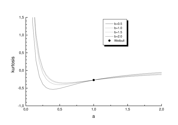
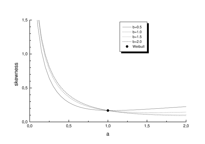
Figure 3: Skewness of the BW distribution as a function of parameter $a$, for several values of parameter $b$

Figure 4: Kurtosis of the BW distribution as a function of parameter $a$, for several values of parameter $b$

Figure 5: Skewness of the BW distribution as a function of parameter $b$, for several values of parameter $a$

Figure 6: Kurtosis of the BW distribution as a function of parameter $b$, for several values of parameter $a$

Graphical representation of skewness and kurtosis for some choices of parameter $b$ as function of parameter $a$, and for some choices of parameter $a$ as function of parameter $b$, for fixed $\lambda=1$ and $c=3$, are given in Figures 3 and 4, and 5 and 6, respectively. It can be observed from Figures 3 and 4 that the skewness and kurtosis curves cross at $a=1$, and from Figures 5 and 6 that both skewness and kurtosis are independent of $b$ for $a=1$. In addition, it should be noted that the Weibull distribution (equivalent to BW for $a=b=1$) is represented by as single point on Figures 3-6.

4 Moment Generating Function

We can give an expansion for the mgf of the BW distribution as follows

$$M(t) = \frac{c\lambda^{c}}{B(a,b)}\int_{0}^{\infty}{\rm exp}(tx)x^{c-1}{\rm exp}\{-b(\lambda x)^{c}\}[1-{\rm exp}\{-(\lambda x)^{c}\}]^{a-1}dx$$

$$= \frac{c\lambda^{c}}{B(a,b)}\sum_{r=0}^{\infty}\frac{t^{r}}{r!}\int_{0}^{\infty}x^{r+c-1}{\rm exp}\{-b(\lambda x)^{c}\}[1-{\rm exp}\{-(\lambda x)^{c}\}]^{a-1}dx$$

$$= \frac{c\lambda^{c}}{B(a,b)}\sum_{r=0}^{\infty}\frac{t^{r}}{r!}\frac{\lambda^{-(r+c)}}{c}S_{r/c+1,b,a},$$

where the last expression comes from (13). For positive real non-integer $a$ using (17) we have

$$M(t)=\frac{\Gamma(a)}{B(a,b)}\sum_{r=0}^{\infty}\sum_{j=0}^{\infty}\frac{t^{r}\Gamma(r/c+1)(-1)^{j}}{\lambda^{r}\Gamma(a-j)(b+j)^{r/c+1}r!j!},$$ (21)

and for integer $a>0$ using (18) we obtain

$$M(t)=\frac{1}{B(a,b)}\sum_{r=0}^{\infty}\frac{t^{r}\Gamma(r/c+1)}{\lambda^{r}r!}\sum_{j=0}^{a-1}\binom{a-1}{j}\frac{(-1)^{j}}{(b+j)^{r/c+1}}.$$ (22)

Note that the expression for the mgf obtained by Choudhury (2005) is a particular case of (21), when $a=\theta$, $\lambda=1/\alpha$ and $b=1$. When $c=1$, we have

$$M(t) = \sum_{r=0}^{\infty}\frac{\lambda^{-r}t^{r}}{cB(a,b)r!}S_{r+1,b,a}$$

$$= \frac{\lambda}{B(a,b)}\int_{0}^{\infty}e^{tx-b\lambda x}(1-e^{-\lambda x})^{a-1}dx.$$

Substituting $y={\rm exp}(-\lambda x)$ in the above integral yields

$$M(t)=\frac{1}{B(a,b)}\int_{0}^{1}y^{b-t/\lambda-1}(1-y)^{a-1}dy$$ (23)

and using the definition of the beta function in (23) we find

$$M(t)=\frac{B(b-t/\lambda,a)}{B(a,b)},$$

which is precisely the expression (3.1) obtained by Nadarajah and Kotz (2006).

5 Estimation and information matrix

Let $Y$ be a random variable with the BW distribution (3). The log-likelihood for a single observation $y$ of $Y$ is given by

$$\ell(\lambda,c,a,b) = {\rm log}(c)+c\,{\rm log}(\lambda)+(c-1){\rm log}(y)-{\rm log}\left\{B(a,b)\right\}-b(\lambda y)^{c}$$

$$+ (a-1){\rm log}[1-{\rm exp}\{-(\lambda y)^{c}\}].$$

The corresponding components of the score vector are:

$$\frac{\partial\ell}{\partial a}=-\left\{\psi\left(a\right)-\psi\left(a+b\right)\right\}+\log\left\{1-{e^{-\left(\lambda\,y\right)^{c}}}\right\},$$ (24)

$$\frac{\partial\ell}{\partial b}=-\left\{\psi\left(b\right)-\psi\left(a+b\right)\right\}-\left(\lambda\,y\right)^{c},$$ (25)

$$\frac{\partial\ell}{\partial c}={\frac{1}{c}}+\log\left(\lambda\,y\right)-b\left(\lambda\,y\right)^{c}\log\left(\lambda\,y\right)+{\frac{\left(a-1\right)\left(\lambda\,y\right)^{c}\log\left(\lambda\,y\right){e^{-\left(\lambda\,y\right)^{c}}}}{1-{e^{-\left(\lambda\,y\right)^{c}}}}}$$ (26)

and

$$\frac{\partial\ell}{\partial\lambda}={\frac{c}{\lambda}}-{\frac{b\,c}{\lambda}}\left(\lambda\,y\right)^{c}+\frac{c\left(a-1\right)\left(\lambda\,y\right)^{c}{e^{-\left(\lambda\,y\right)^{c}}}}{\lambda\,\left\{1-{e^{-\left(\lambda\,y\right)^{c}}}\right\}}.$$ (27)

The maximum likelihood equations derived by equating (24)-(27) to zero can be solved numerically for $a,b,c$ and $\lambda$. We can use iterative techniques such as a Newton-Raphson type algorithm to obtain the estimates of these parameters. It may be worth noting from $E(\partial\ell/\partial b)=0$, that (25) yields

$$E(Y^{c})=\frac{\psi\left(a+b\right)-\psi\left(b\right)}{\lambda^{c}},$$

which agrees with the previous calculations.

For interval estimation of $(a,b,c,\lambda)$ and hypothesis tests, the Fisher information matrix is required. For expressing the elements of this matrix it is convenient to introduce an extension of the integral (12)

$$T_{d,b,a,e}=\int_{0}^{\infty}{x^{d-1}e^{-bx}\left(1-e^{-x}\right)^{a-1}\left(\log x\right)^{e}dx},$$ (28)

so that we have

$$T_{d,b,a,0}=S_{d,b,a}.$$

As before, let $W=-\log(U)$, where $U$ is a random variable following the Beta$(b,a)$ distribution, then

$$E[W^{d-1}\{\log(W)\}^{e}] = \int_{-\infty}^{\infty}x^{d-1}(\log x)^{e}dF_{W}(x)$$

$$= \frac{1}{B(a,b)}\int_{0}^{\infty}x^{d-1}e^{bx}(1-e^{-x})^{a-1}(\log x)^{e}dx$$

$$= \frac{T_{d,b,a,e}}{B(a,b)}.$$

Hence, the equation

$$T_{d,b,a,e}=B(a,b)E[W^{d-1}\{\log(W)\}^{e}],$$ (29)

relates $T_{d,b,a,e}$ to expected values.

To simplify the expressions for some elements of the information matrix, it is useful to note the identities

$$S_{1,b+2,a}-2S_{1,b+1,a}+S_{1,b,a}=B(a+2,b)$$

and

$$bS_{2,b,a}-(a+2b+1)S_{2,b+1,a}+(a+b+1)S_{2,b+2,a}=B(a+2,b),$$

which can be easily proved.

Explicit expressions for the elements of the information matrix $K$, obtained using Maple and Mathematica algebraic manipulation software (we have used both for double checking the obtained expressions), are given below in terms of the integrals (12) and (28):

$$\kappa_{a,a}=\psi^{\prime}\left(a\right)-\psi^{\prime}\left(a+b\right),$$

$$\kappa_{a,b}=-\psi^{\prime}\left(a+b\right),~{}\kappa_{a,c}=-{\frac{T_{{2,b+1,a-1,1}}}{cB\left(a,b\right)}},~{}\kappa_{a,\lambda}=-{\frac{c\,S_{{2,b+1,a-1}}}{\lambda B\left(a,b\right)}},$$

$$\kappa_{b,b}=\psi^{\prime}\left(b\right)-\psi^{\prime}\left(a+b\right),~{}\kappa_{b,c}={\frac{T_{{2,b,a,1}}}{cB\left(a,b\right)}},~{}\kappa_{b,\lambda}=\frac{c}{\lambda}{\frac{S_{{2,b,a}}}{B\left(a,b\right)}},$$

$$\kappa_{c,c}= \frac{1}{{c}^{2}}+\frac{1}{c^{2}\,B\left(a,b\right)}\left\{\left(a-1\right)T_{{3,b+1,a-2,2}}\right.$$

$$\left.+b\,T_{{2,b,a-2,2}}-\left(a+2\,b-1\right)T_{{2,b+1,a-2,2}}+\left(a+b-1\right)T_{{2,b+2,a-2,2}}\right\},$$

$$\kappa_{c,\lambda}= \frac{1}{\lambda\,B\left(a,b\right)}\left\{\left(a-1\right)T_{{3,b+1,a-2,1}}\right.$$

$$\left.+b\,T_{{2,b,a-2,1}}-\left(a+2\,b-1\right)T_{{2,b+1,a-2,1}}+\left(a+b-1\right)T_{{2,b+2,a-2,1}}\right\}$$

and

$$\kappa_{\lambda,\lambda}= \frac{c^{2}}{{\lambda}^{2}}+\frac{{c}^{2}\left(a-1\right)}{{\lambda}^{2}B\left(a,b\right)}S_{{3,b+1,a-2}}.$$

The integrals $S_{{i,j,k}}$ and $T_{{i,j,k,l}}$ in the information matrix are easily numerically determined using MAPLE and MATHEMATICA for any $a$ and $b$.

Under conditions that are fulfilled for parameters in the interior of the parameter space but not on the boundary, the asymptotic distribution of the maximum likelihood estimates $\hat{a},\hat{b},\hat{c}$ and $\hat{\lambda}$ is multivariate normal $N_{4}(0,K^{-1})$. The estimated multivariate normal $N_{4}(0,\widehat{K}^{-1})$ distribution can be used to construct approximate confidence intervals and confidence regions for the individual parameters and for the hazard rate and survival functions. The asymptotic normality is also useful for testing goodness of fit of the BW distribution and for comparing this distribution with some of its special sub-models using one of the three well-known asymptotically equivalent test statistics - namely, the likelihood ratio (LR) statistic, Wald and Rao score statistics.

We can compute the maximum values of the unrestricted and restricted log-likelihoods to construct the LR statistics for testing some sub-models of the BW distribution. For example, we may use the LR statistic to check if the fit using the BW distribution is statistically “superior” to a fit using the exponentiated Weibull or Weibull distributions for a given data set. Mudholkar et al. (1995) in their discussion of the classical bus-motor-failure data, noted the curious aspect in which the larger EW distribution provides an inferior fit as compared to the smaller Weibull distribution.

6 Application to real data

In this section we compare the results of fitting the BW and Weibull distribution to the data set studied by Meeker and Escobar (1998, p. 383), which gives the times of failure and running times for a sample of devices from a field-tracking study of a larger system. At a certain point in time, 30 units were installed in normal service conditions. Two causes of failure were observed for each unit that failed: the failure caused by an accumulation of randomly occurring damage from power-line voltage spikes during electric storms and failure caused by normal product wear. The times are: 275, 13, 147, 23, 181, 30, 65, 10, 300, 173, 106, 300, 300, 212, 300, 300, 300, 2, 261, 293, 88, 247, 28, 143, 300, 23, 300, 80, 245, 266.

The maximum likelihood estimates and the maximized log-likelihood $\hat{l}_{BW}$ for the BW distribution are:

$$\hat{a}=0.0785,\hat{b}=0.0659,\hat{c}=7.9355,\hat{\lambda}=0.004987\hbox{~{}~{}and~{}~{}}\hat{l}_{BW}=-169.919,$$

while the maximum likelihood estimates and the maximized log-likelihood $\tilde{l}_{W}$ for the Weibull distribution are:

$$\tilde{c}=1.2650,\tilde{\lambda}=0.005318\hbox{~{}~{}and~{}~{}}\tilde{l}_{W}=-184.3138.$$

The likelihood ratio statistic for testing the hypothesis $a=b=1$ (namely, Weibull versus BW distribution) is then $w=28.7896$, which indicates that the Weibull distribution should be rejected. As an alternative test we use the Wald statistic. The asymptotic covariance matrix of the maximum likelihood estimates for the BW distribution, which comes from the inverse of the information matrix, is given by

$$\widehat{K}^{-1}=10^{-7}\times\left(\begin{array}[]{rrrr}8699.35364&4743.69977&-488130.870&87.9136383\\ 4743.69977&13079.4394&-4009.69885&-135.603333\\ -488130.870&-4009.69885&58517447.8&-16222.8149\\ 87.9136383&-135.603333&-16222.8149&6.19530131\end{array}\right).$$

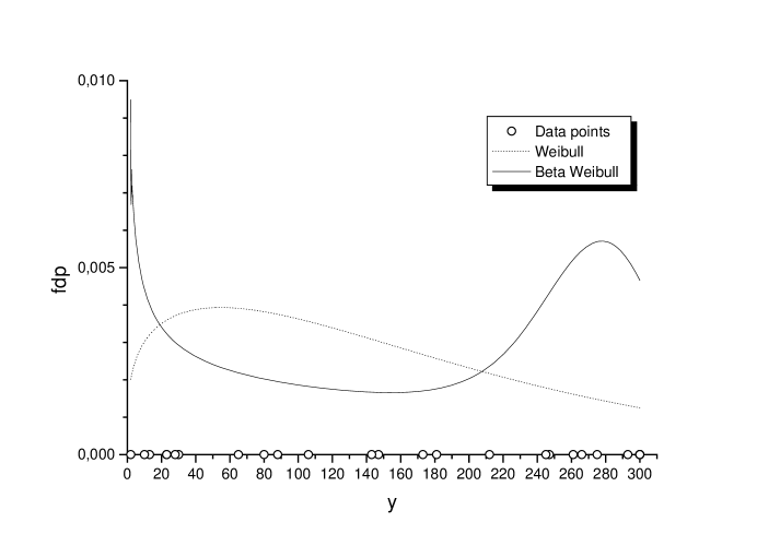
The resulting Wald statistic is found to be $W=38.4498$, again signalizing that the BW distribution conform to the above data. In Figure 7 we display the pdf of both Weibull and BW distributions fitted and the data set, where it is seen that the BW model captures the aparent bimodality of the data.

Figure 7: The probability density function (3) of the fitted BW and Weibull distributions

7 Conclusion

The Weibull distribution, having exponential and Rayleigh as special cases, is a very popular distribution for modeling lifetime data and for modeling phenomenon with monotone failure rates. In fact, the BW distribution represents a generalization of several distributions previously considered in the literature such as the exponentiated Weibull distribution (Mudholkar et al., 1995, Mudholkar and Hutson, 1996, Nassar and Eissa, 2003, Nadarajah and Gupta, 2005 and Choudhury, 2005) obtained when $b=1$. The Weibull distribution (with parameters $c$ and $\lambda$) is also another particular case for $a=1$ and $b=1$. When $a=1$, the BW distribution reduces to a Weibull distribution with parameters $\lambda\,b^{1/c}$ and $c$. The beta exponential distribution is also an important special case for $c=1$.

The BW distribution provides a rather general and flexible framework for statistical analysis. It unifies several previously proposed families of distributions, therefore yielding a general overview of these families for theoretical studies, and it also provides a rather flexible mechanism for fitting a wide spectrum of real world data sets.

We derive explicit expressions for the moments of the BW distribution, including an expansion for the moment generating function. These expressions are manageable and with the use of modern computer resources with analytic and numerical capabilities, may turn into adequate tools comprising the arsenal of applied statisticians. We discuss the estimation procedure by maximum likelihood and derive the information matrix. Finally, we demonstrate an application to real data.

Appendix

In what follows, we derive the identities (17) and (18). We start from

$$f(x)={\rm exp}(-bx)(1-e^{-x})^{a-1},$$

which yields

$$\int_{0}^{\infty}x^{d-1}f(x)dx=\int_{0}^{\infty}x^{d-1}{\rm exp}(-bx)(1-e^{-x})^{a-1}dx,$$

and substituting $z=e^{-x}$ gives

$$\int_{0}^{\infty}x^{d-1}f(x)dx=\int_{0}^{1}|{\rm log}z|^{d-1}z^{b-1}(1-z)^{a-1}dz.$$ (30)

For real non-integer $a$, we have

$$\int_{0}^{\infty}x^{d-1}f(x)dx=\Gamma(a)\sum_{j=0}^{\infty}\frac{(-1)^{j}}{\Gamma(a-j)j!}\int_{0}^{1}|{\rm log}z|^{\gamma/c-1}z^{b+j-1}dz.$$

Also, for real $p>-1$ and real $q$, we have

$$\int_{0}^{1}x^{p}|{\rm log}x|^{q}dx=\frac{\Gamma(1+q)}{(1+p)^{q+1}}.$$ (31)

Hence,

$$\int_{0}^{\infty}x^{d-1}f(x)dx=\Gamma(a)\sum_{j=0}^{\infty}\frac{(-1)^{j}\Gamma(d)}{\Gamma(a-j)j!(b+j)^{d}},$$

and, finally, we arrive at

$$\int_{0}^{\infty}x^{d-1}{\rm exp}(-bx)(1-e^{-x})^{a-1}dx=\Gamma(a)\Gamma\left(d\right)\sum_{j=0}^{\infty}\frac{(-1)^{j}}{\Gamma(a-j)j!(b+j)^{d}},$$

which represents the identity (17).

Now, let $a>0$ be an integer; then, from (30), we have

$$\int_{0}^{\infty}x^{d-1}f(x)dx=\sum_{j=0}^{a-1}\binom{a-1}{j}{(-1)^{j}}\int_{0}^{1}|{\rm log}z|^{d-1}z^{b+j-1}dz.$$

Using (31) we obtain

$$\int_{0}^{\infty}x^{d-1}f(x)dx=\sum_{j=0}^{a-1}\binom{a-1}{j}\frac{(-1)^{j}\Gamma(d)}{(b+j)^{d}},$$

and therefore we arrive at

$$\int_{0}^{\infty}x^{d-1}{\rm exp}(-bx)(1-e^{-x})^{a-1}dx=\Gamma\left(d\right)\sum_{j=0}^{a-1}\binom{a-1}{j}\frac{(-1)^{j}}{(b+j)^{d}},$$

which represents the identity (18).

References

• [1] Brown, B. W., Spears, F. M. and Levy, L. B. (2002). The log F𝐹F: a distribution for all seasons. Comput. Statist., 17, 47-58.
• [2] Choudhury, A., 2005. A simple derivation of moments of the exponentiated Weibull distribution. Metrika, 62, 17-22.
• [3] Eugene, N., Lee, C. and Famoye, F., 2002. Beta-normal distribution and its applications. Commun. Statist. - Theory and Methods, 31, 497-512.
• [4] Famoye, F., Lee, C. and Olumolade, O., 2005. The Beta-Weibull Distribution. J. Statistical Theory and Applications, 4, 121-136.
• [5] Gupta, R. D. and Kundu, D., 2001. Exponentiated Exponential Family: An Alternative to Gamma and Weibull Distributions. Biometrical Journal, 43, 117-130.
• [6] Gupta, A. K. and Nadarajah, S., 2004. On the moments of the beta normal distribution. Commun. Statist. - Theory and Methods, 33, 1-13.
• [7] Jones, M. C., 2004. Families of distributions arising from distributions of order statistics. Test, 13, 1-43.
• [8] Lawless, J. F., 1982. Statistical Models and Methods for Lifetime Data. John Wiley, New York.
• [9] Lee, C., Famoye, F. and Olumolade, O., 2007. Beta-Weibull Distribution: Some Properties and Applications to Censored Data. J. Modern Applied Statistical Methods, 6, 173-186.
• [10] Linhart, H. and Zucchini, W., 1986. Model Selection. John Wiley, New York.
• [11] Meeker, W. Q. and Escobar, L. A., 1998. Statistical Methods for Reliability Data. John Wiley, New York.
• [12] Mudholkar, G. S., Srivastava, D. K. and Freimer, M., 1995. The exponentiated Weibull family. Technometrics, 37, 436-45.
• [13] Mudholkar, G. S. and Hutson, A. D., 1996. The exponentiated Weibull family: some properties and a flood data application. Commun. Statist. - Theory and Methods, 25, 3059-3083.
• [14] Nadarajah, S. and Gupta, A. K., 2005. On the moments of the exponentiated Weibull distribution. Commun. Statist. - Theory and Methods, 34, 253-256.
• [15] Nadarajah, S. and Kotz, S., 2004. The beta Gumbel distribution. Math. Probab. Eng., 10, 323-332.
• [16] Nadarajah, S. and Kotz, S., 2006. The beta exponential distribution. Reliability Engineering and System Safety, 91, 689-697.
• [17] Nassar, M. M. and Eissa, F. H., 2003. On the exponentiated Weibull distribution. Commun. Statist. - Theory and Methods, 32, 1317-1336.