Calculation of Asymptotic and RMS
Kicks due to Higher Order Modes
in the 3.9 GHz Cavity

Abstract

FLASH plans to use a “third harmonic” ($3.9$ GHz) superconducting cavity to compensate nonlinear distortions of the longitudinal phase space due to the sinusoidal curvature of the the cavity voltage of the TESLA $1.3$ GHz cavities. Higher order modes (HOMs) in the $3.9$ GHz have a significant impact on the dynamics of the electron bunches in a long bunch train. Kicks due to dipole modes can be enhanced along the bunch train depending on the frequency and Q-value of the modes. The enhancement factor for a constant beam offset with respect to the cavity has been calculated. A simple Monte Carlo model of these effects, allowing for scatter in HOM frequencies due to manufacturing variances, has also been implemented and results for both FLASH and for an XFEL-like configuration are presented.

1 Introduction

FLASH plans to use a “third harmonic” ($3.9$ GHz) superconducting cavity to compensate nonlinear distortions of the longitudinal phase space due to the sinusoidal curvature of the the cavity voltage of the TESLA $1.3$ GHz cavities. Higher order modes (HOMs) in the $3.9$ GHz have a significant impact on the dynamics of the electron bunches in a long bunch train. The analysis here seeks to determine what level of damping, if any, is required.

In the case where the spacing of the bunches is near (but not exactly the same as) a multiple of the period of a dipole HOM, kicks from the HOM can be resonantly enhanced along the bunch train, depending on the frequency and Q-value of the modes. The enhancement factor for a constant beam offset with respect to the cavity can be expressed in a simple analytic form, which also provides the energy loss from resonance effects with a monopole mode.

A simple Monte Carlo model of these effects, allowing for scatter in HOM frequencies due to manufacturing variances, has also been implemented and results for both a FLASH-like and for an XFEL-like configuration are presented.

The beam parameters for our analyses are:

Parameter	FLASH	XFEL-like injector
Bunch spacing	$1\mu s$	$200ns$
Bunch charge	$1nC$	$1nC$
Bunch length (1$\sigma$)	$1ps$	$1ps$
Beam energy	$130\,\mathrm{M}eV$	$500\,\mathrm{M}eV$
Bunch offset at entry	$1mm$	$1mm$
Bunches per train	800	800
Number of cavities	4	32

Table 1: Beam parameters for typical FLASH and XFEL injector running.

An important issue is the specification for how much kick can be tolerated before lasing stops. At FLASH, the spot size at the location where the “third harmonic” cavities will be installed is about 0.2mm and the invariant emittance’s design value is 1 mm-mrad in both $x$ and $y$; in real operation it is often twice that. The beam divergence is thus about 20$\mu$rad in the best case. We use $\pm 10\mu$rad as our target. We do not have a target for energy loss, but find small values for these effects in all cases.

Although we are primarily concerned with FLASH, our methods are completely general and we have done some investigation of the situation for XFEL. The optics for the XFEL are in a state of flux at this writing; our selection of parameters here is perforce somewhat arbitrary. The $\pm 10\mu$rad requirement is not far from other parameter sets that are under consideration at this writing. A more detailed study of the XFEL requirements is being undertaken by Yauhen Kot and Thorsten Limberg. We do not here allow for betatron phase advance between the cavities, and this effect will be larger at the XFEL than at FLASH.

2 Wakefield due to HOMs

The purpose of this section is to define the parameters that are important for the long range wake field calculation. Our development follows reference [1] closely.

2.1 Modes in a cavity

2.1.1 The electric and magnetic fields

Consider a monopole ($m=0$) or dipole mode ($m=1$) mode with the frequency $f=\omega/(2\,\pi)$ in a cavity with cylindrical symmetry. One obtains in complex notation for the electric and magnetic field:

$$\mbox{ \boldmath$E$ }(r,\phi,z,t) = \begin{array}[t]{ll}\left(\,\,\widetilde{E_{r}^{(m)}}(r,z)\right.\,\cos(m\,\phi)&\mbox{ \boldmath$e_{r}$ }\\ \vspace*{1mm}+\,\,\widetilde{E_{\phi}^{(m)}}(r,z)\,\sin(m\,\phi)&\mbox{ \boldmath$e_{\phi}$ }\\ +\,\,\widetilde{E_{z}^{(m)}}(r,z)\,\cos(m\,\phi)&\mbox{ \boldmath$e_{z}$ }\left.\phantom{\widetilde{E_{r}^{(m)}}}\right)\,\exp(-i\,\omega\,t)\\ \end{array}$$ (4)

$$\mbox{ \boldmath$B$ }(r,\phi,z,t) = \begin{array}[t]{ll}\left(\,\,\widetilde{B_{r}^{(m)}}(r,z)\right.\,\sin(m\,\phi)&\mbox{ \boldmath$e_{r}$ }\\ +\,\,\widetilde{B_{\phi}^{(m)}}(r,z)\,\cos(m\,\phi)&\mbox{ \boldmath$e_{\phi}$ }\\ +\,\,\widetilde{B_{z}^{(m)}}(r,z)\,\sin(m\,\phi)&\mbox{ \boldmath$e_{z}$ }\left.\phantom{\widetilde{E_{r}^{(m)}}}\right)\,\exp(-i\,\omega\,t).\\ \end{array}$$ (9)

2.1.2 The loss parameter and $R/Q$

The interaction of the beam with a cavity mode is characterized by the loss parameter $k^{(m)}_{\|}(r)$ or by the quantity $R/Q$ [2]. These parameters can be determinated from the numerically calculated fields using the MAFIA post-processor [3, 4]. The longitudinal voltage for a given mode at a fixed radius $r$ is defined as

$$V^{(m)}_{\|}(r)=\int_{0}^{L}\,dz\,\widetilde{E_{z}^{(m)}}(r,z)\exp(-i\,\omega\,z/c),$$ (10)

while the total stored energy is given by:

$$U^{(m)}=\frac{\epsilon_{0}}{2}\,\,\int d^{3}r\,\,\left|\widetilde{\mbox{ \boldmath$E^{(m)}$ }}\right|^{2}.$$ (11)

From the voltage and stored energy the loss parameter and $R/Q$ can be calculated:

$$k^{(m)}(r) = \frac{\left|V^{(m)}_{\|}(r)\right|^{2}}{4\,U^{(m)}}$$

$$\frac{R^{(m)}}{Q} = \frac{1}{r^{2\,m}}\frac{2\,\,k^{(m)}(r)}{\omega}.$$

For monopole modes the superscript $(0)$ is usually omitted $R/Q=R^{(0)}/Q$. Although our definitions include a radial dependence in the loss parameter, $R^{(m)}/Q$ is independent of the radius $r$ since it can be shown (see [2, 5]) that $V^{(m)}(r)\sim r^{m}$ and therefore $k^{(m)}(r)\sim r^{2\,m}$.

2.1.3 The geometry parameter $G_{1}$ and the Q-value

The power $P_{sur}$ dissipated into the cavity wall due to the surface resistivity $R_{sur}$ can be calculated from the tangential magnetic field:

$$P_{sur}=\frac{1}{2}\,\,R_{sur}\,\,\int dA\left|H_{sur}\right|^{2}.$$ (13)

For a superconducting cavity the surface resistance is the sum of the BCS (Bardeen, Cooper, Schrieffer) resistance $R_{BCS}$, which depends on the frequency and the temperature, and a residual resistivity $R_{0}$. The BCS resistance $R_{BCS}$ scales with the square of the frequency $f$ and exponentially with the temperature $T$:

$$R_{BCS}(f,T)\propto\frac{f^{2}}{T}\,\exp(-1.76\,T_{c}/T).$$ (14)

The less-well understood residual resistance $R_{0}$ adds directly to $R_{BCS}$ but remains in the limit $T\rightarrow 0$.

The total damping of a cavity mode is not only determined by the surface losses but also by coupling to external waveguides (HOM-dampers). Therefore one has to distinguish the Q-value $Q_{0}$ which is defined above and the external Q-value $Q_{ext}$ which characterizes the coupling to external waveguides. Typically, $Q_{0}>>Q_{ext}$.

The geometry parameter $G_{1}$ [6] is defined as:

$$G_{1}=R_{sur}\,\,Q_{0}.$$ (15)

$G_{1}$ is a purely geometric quantity that is independent of the cavity material; it depends only on the mode and the shape of the cavity that creates that mode.

2.2 Wakefields

2.2.1 Wake potential

Figure 1: A point charge $q_{1}$ traversing a cavity with an offset $r_{1}$ followed by a test charge $q_{2}$ with offset $r_{2}$ .

Consider the situation shown in Figure 1. A test charge $q_{2}$ follows a point charge $q_{1}$ at a distant $s$. The distant $s$ is positive in the direction opposite to the motion of the point charge $q_{1}$. Both charges are relativistic ($v\approx c$). The Lorentz force on the test charge due to the fields generated by the point charge $q_{1}$ is

$$\mbox{ \boldmath$F$ }=\frac{d\mbox{ \boldmath$p$ }}{dt}=\,\,q_{2}\,(\mbox{ \boldmath$E$ }+c\,\mbox{ \boldmath$e_{z}$ }\times\mbox{ \boldmath$B$ }).$$ (16)

The wake potential of the point charge $q_{1}$ is defined as:

$$\mbox{ \boldmath$W$ }(x_{2},y_{2},x_{1},y_{1},s)=\frac{1}{q_{1}}\,\,\int_{0}^{L}dz(\mbox{ \boldmath$E$ }+c\,\mbox{ \boldmath$e_{z}$ }\times\mbox{ \boldmath$B$ })_{t=(z+s)/c}.$$ (17)

The wake potential is the integrated Lorentz force on a test charge. Causality requires $\mbox{ \boldmath$W$ }(s)=0$ for $s<0$.

The longitudinal and transverse components of the wake potential are connected by the Panofsky-Wenzel theorem [7]

$$\frac{\partial}{\partial s}\mbox{ \boldmath$W$ }_{\bot}(x_{2},y_{2},x_{1},y_{1},s)=-\mbox{ \boldmath$\nabla$ }_{\bot_{2}}W_{\|}(x_{2},y_{2},x_{1},y_{1},s).$$ (18)

Integration of the transverse gradient (applied to the transverse coordinates of the test charge) of the longitudinal wake potential yields the transverse wake potential.

2.2.2 Multipole expansion of the wake potential

If the structure traversed by the bunch is cylindrically symmetric then a multipole expansion can be used to describe the wake potential. The location of the bunch train in the $(r,\phi)$ plane will break the symmetry and determine the azimuthal orientation of the $m>0$ modes. Consider again the situation shown in Figure 1. Assume that the point charge $q_{1}$ traverses the cavity at position $(r_{1},\varphi_{1})$, while the test charge follows at position $(r_{2},\varphi_{2})$. The longitudinal wake potential may be expanded in multipoles:

$$W_{\|}(r_{1},r_{2},\varphi_{1},\varphi_{2},s)=\sum_{m=0}^{\infty}\,{r_{1}}^{m}\,{r_{2}}^{m}\,\,W^{(m)}_{\|}(s)\,\,\cos m\,(\varphi_{2}-\varphi_{1}).$$ (19)

The functions $W^{(m)}_{\|}(s)$ are the longitudinal $m$-pole wake potentials. There is no a-priori relation between the wake potentials of different azimuthal order $m$.

The transverse wake potential can be calculated using the Panofsky-Wenzel theorem, and the transverse $m$-pole wake potentials are defined as:

$$W^{(m)}_{\bot}(s)=-\int_{-\infty}^{s}ds^{\prime}\,W^{(m)}_{\|}(s^{\prime}),$$ (20)

for $m>0$. There is no transverse monopole wake potential. The dipole wake potential does not depend on the position of the test charge $q_{2}$. The kick on the test charge is linear in the offset of the point charge $q_{1}$.

2.2.3 Wakefields due to HOMs

It is possible to write the m-pole wake potentials $W^{(m)}_{\|}(s)$ as a sum over all modes:

$$W^{(m)}_{\|}(s) = -\sum_{n}\,\,\omega_{n}{\left(\frac{R^{(m)}}{Q}\right)}_{n}\cos(\omega_{n}\,s/c)\,\,\exp(-1/{\tau_{n}}\,\,s/c)$$

$$W^{(m)}_{\bot}(s) = c\,\sum_{n}\,\,{\left(\frac{R^{(m)}}{Q}\right)}_{n}\sin(\omega_{n}\,s/c)\,\,\exp(-1/{\tau_{n}}\,\,s/c).$$

where $\omega_{n}$ are the frequencies of the m-pole modes. A damping term has been included with the damping time $\tau_{n}$ for mode $n$. As $Q_{0}>>Q_{ext}$, the damping time of the voltage is very nearly

$$\tau_{n}\approx\frac{2\,(Q_{ext})_{n}}{\omega_{n}}.$$ (22)

3 Effects of long range wakefields on a bunch train

3.1 Energy deviations and kicks on the bunches

The long range wakes due to HOMs can cause energy deviations and kicks on the bunches. A bunch train of $N$ bunches is shown in Figure 2; the notation for the offsets with respect to the reference axis of the accelerator is $x_{i}$ and $y_{i}$ and the direction of the longitudinal coordinate $s$ ($s=0$ at the first bunch of the train) is also shown. It is assumed that all bunches have the same bunch charge $q$. In our investigation of the energy deviation and the kick on the bunch $n$ within the bunch train we profited strongly from the analysis of long range wakes and beam loading by P. Wilson [6].

Figure 2: Schematic representation of a train of bunches with offsets $x_{i}$ and $y_{i}$ with respect to the reference axis of the accelerator.

The energy deviation of bunch $n$ due to HOMs is a sum over all HOMs produced by all preceding bunches in the train. Additionally the the self-wake due to HOMs is also included ($W^{(0)}_{\|}(0)$ and $W^{(1)}_{\|}(0)$), which is the HOM equivalent of the fundamental theorem of beam loading [6].

$$\Delta E(s_{n}) = e\,q\,W^{(0)}_{\|}(0)$$

$$+e\,q\sum_{j<n}\,W^{(0)}_{\|}(s_{n}-s_{j})$$

$$+e\,q\,({x_{n}}^{2}+{y_{n}}^{2})W^{(1)}_{\|}(0)$$

$$+e\,q\sum_{j<n}\,\,(x_{n}\,x_{j}+y_{n}\,y_{j})\,\,W^{(1)}_{\|}(s_{n}-s_{j})$$

$$+\dots$$

As an example the energy deviation due the selfwake of a higher monopole mode with a frequency of $f=6$ GHz is considered. The contribution to the energy deviation for a bunch with a population of $N=6.5\times 10^{9}$ electrons is given by:

$$\Delta E=e\,1\,{\rm nC}\,\,\,2\,\pi\,\,6\,{\rm GHz}\,\,\frac{1}{2}\,\,\frac{R}{Q}.$$ (24)

An energy deviation of $196$ eV corresponds to an impedance ($R/Q$) of 10 $\Omega$ and a loss parameter of $k^{(0)}_{\|}=0.188$ V/pC. The factor $1/2$ is a consequence of the fundamental theorem of beam loading.

Now consider the transverse long range wakefields. The kick on bunch $n$ due to the dipole wake field is:

$$\mbox{ \boldmath$\theta$ }_{n} = \frac{e\,q_{bunch}}{E_{beam}}\,\,\sum_{j<n}\,\,(x_{j}\,\,\mbox{ \boldmath$e_{x}$ }+y_{j}\,\,\mbox{ \boldmath$e_{y}$ })W^{(1)}_{\bot}(s_{n}-s_{j})$$

$$+\dots,$$

where $E_{n}$ is the energy of bunch. The kick on bunch $n$ due to one dipole mode with revolution frequency $\omega_{1}$ and damping constant $\tau_{1}$ is:

$$\mbox{ \boldmath$\theta$ }_{n}=\widehat{\theta}_{n}\,\,\sum_{j<n}\,\,(\frac{x_{j}}{x_{0}}\,\,\mbox{ \boldmath$e_{x}$ }+\frac{y_{j}}{x_{0}}\,\,\mbox{ \boldmath$e_{y}$ })\sin(\omega_{1}\,(s_{n}-s_{j})/c)\,\,\exp(-1/{\tau_{1}}\,\,(s_{n}-s_{j})/c),$$ (26)

where the kick amplitude $\widehat{\theta}_{n}$ on bunch $n$ is defined as

$$\widehat{\theta}_{n}=\frac{e\,q_{bunch}}{E_{beam}}\,c\,\frac{R^{(1)}}{Q}\,r_{0},$$ (27)

with respect to an arbitrary reference offset $r_{0}$.

3.2 One dipole mode and a bunch train with constant offset

It is instructive to consider the simplified situation of a bunch with a constant offset with respect to the “third harmonic” cavity. This corresponds to an injection error or an misalignment of the cavity. Since the long range dipole wakefield is a linear superposition of HOMs it is sufficient to consider only one mode at a time in all analytical formulas.

Modes from the first 3 dipole passbands with the highest values for $R^{(1)}/Q$ are summarized in table 2, taken from reference [8], along with high $R^{(m)}/Q$ modes of other azimuthal number. The kick amplitude $\widehat{\theta}$ for the dipole modes has been calculated according to Equation 27 assuming that all bunches have the same energy of 130 MeV, bunch charge of 1 nC and reference offset of 1 mm.

$f$ / GHz $m$ $R^{(m)}/Q$ / $G_{1}$ / $k^{(m)}/r_{0}^{(2m)}$ / $\widehat{\theta}$ / $\mu$rad $\Omega/{\rm cm}^{(2m)}$ $\Omega$ ${\rm V}/({\rm pC}\,{\rm cm}^{(2m)})$ 7.506 0 23.3 475.5 0.55 4.834 1 50.7 277.3 0.77 1.22 5.443 1 20.9 426.2 0.36 0.50 7.669 1 29.5 470.7 0.71 0.71 9.133 2 11.2 402.9 0.32

Table 2: RF-parameters and kick amplitude of modes with high $R^{(m)}/Q$. For the dipole modes ($m=1$), the kick amplitude has been calculated for an beam energy of 130 MeV, a bunch charge of 1 nC and an reference offset ($r_{0}$) of 1 mm.

Furthermore it is now assumed that the bunch to bunch distance $\Delta t$ is constant:

$$\Delta t=\frac{\Delta s}{c}=n_{fb}\,\frac{1}{f_{fu}},$$ (28)

where $f_{fu}=3.9$ GHz is the frequency of the fundamental mode and $n_{fb}$ is the number of free buckets between bunches. The following bunch distances have to be considered for the operation of the injector linear accelerator:

$\Delta t$ / ns $1/\Delta t$ / MHz $n_{fb}$ 200 5.0 780 1000 1.0 3900 2000 0.5 7800 10000 0.1 39000

Table 3: Typical bunch to bunch distance for the operation of injector linear accelerator

The bunch distance can be translated into a phase distance $\delta$ between bunches:

$$\delta=\omega_{1}\,\Delta t=2\pi\frac{f_{1}}{f_{fu}}\,n_{fb},$$ (29)

where $\omega_{1}=2\pi\,f_{1}$ is the frequency of the considered dipole mode.

A small change in the dipole frequency due to fabrication tolerances will cause a large change in the bunch to bunch phase since the number of free buckets is relatively large. One obtains for a bunch distance of $1/\Delta t=1{\rm MHz}$:

$$\Delta\delta = 2\pi\frac{1}{f_{fu}}\,n_{fb}\,\,\Delta f_{1}$$ (30)

$$= 0.36^{\circ}\,\frac{\Delta f_{1}}{{\rm kHz}}$$ (31)

A change of $10^{\circ}$ in the bunch to bunch phase after $n_{fb}=3900$ free buckets corresponds to a frequency shift of about 20 kHz, which is much smaller than the expected variation due to manufacturing variations.

A bunch to bunch damping constant for the kick voltage is defined as:

$$d=\frac{\omega_{1}}{2\,Q_{1}}\,\Delta t=2\pi\frac{f_{1}}{f_{fu}}\,n_{fb}\,\frac{1}{2\,Q_{1}},$$ (32)

where $Q_{1}$ is the Q-value of the dipole mode, which is usually dominated by the external Q-value of the HOM damper. We give most of our expressions both in terms of $d$ and of $a=e^{-d}$. A plot of the damping constant as a function of the Q-value is shown in Figure 3 in a double logarithmic scale for the three modes considered in table 2 and a bunch to bunch spacing of $1/\Delta t=1$ MHz.

Figure 3: The damping constant d versus the Q-value for the three dipole modes from table 2. Additionally the damping constants $d=0.5$ and $d=0.15$ are indicated with parallel lines.

With HOM dampers Q-values of about $10^{5}$ are achieved, which corresponds to a damping constant of about $0.15$ ($1/\Delta t=1$ MHz). If no HOM-dampers are mounted on the cavity the Q-value will be larger than $10^{9}$ and the damping constant $d$ will be very small ($\sim 10^{-5}$). Some details of the damping constants for the modes from Table 2 are listed in the Table 4.

$1/\Delta t=1$ MHz $1/\Delta t=5$ MHz $f$ / GHz Q-Value Q-Value $10^{4}$ $5\times 10^{4}$ $10^{5}$ $10^{4}$ $5\times 10^{4}$ $10^{5}$ 4.834 1.5 0.30 0.15 0.30 0.06 0.04 5.443 1.7 0.34 0.17 0.34 0.07 0.03 7.669 2.4 0.48 0.24 0.48 0.10 0.05

Table 4: Damping constants $d$ for three modes and different external Q-value and bunch-to-bunch distances of $1000$ ns and $200$ ns.

Using the above defined parameters $\delta$ and $d$, the energy deviation and the kick on bunch $n\in\{1,2,3\ldots\}$ due to one dipole mode are:

$$\Delta E_{n} = \widehat{E}\left(\frac{1}{2}+\sum_{j=1}^{n-1}\cos(\delta\,(n-j))\,\exp(-d\,(n-j))\right),$$ (33)

$$\theta_{n} = \widehat{\theta}\,\,\,\sum_{j=1}^{n-1}\sin(\delta\,(n-j))\,\exp(-d\,(n-j)),$$ (34)

where

$$\widehat{E}=-e\,q\,\omega_{1}\frac{R^{(1)}}{Q}\,{r_{0}}^{2},\hskip 14.22636pt{\rm and}\hskip 14.22636pt\widehat{\theta}=\frac{e\,q}{E_{0}/c}\,\frac{R^{(1)}}{Q}\,r_{0}.$$ (35)

$r_{0}$ is a reference offset. The above expression (33) and (34) can be rewritten as

$$\Delta E_{n} = \widehat{E}\left(\frac{1}{2}+{\rm Re}\left(S_{n}\right)\right),$$

$$\theta_{n} = \widehat{\theta}\,\,\,{\rm Im}\left(S_{n}\right),$$ (36)

with a sequence of complex sums $S_{n}$, defined as

$$S_{n}=\sum_{j=1}^{n-1}\exp\left((n-j)\,D\right)=\sum_{j=1}^{n-1}\exp\left(j\,D\right).$$ (37)

The complex damping constant $D$ is defined as $D=i\,\delta-d$. The sequence $S_{n}$ may be calculated via a recurrence relation:

$$S_{1} = 0$$ (38)

$$S_{n+1} = \left(S_{n}+1\right)\exp(D),$$

or via an explicit expression for the sum of a geometric series:

$$S_{n}=\frac{1-\exp((n-1)\,D)}{\exp(-D)-1}\longrightarrow\frac{1}{\exp(-D)-1},\,\,{\rm for}\,\,n\rightarrow\infty.$$ (39)

Furthermore let $R_{n}$ be defined as:

$$R_{n}=\frac{\exp((n-1)\,D)}{\exp(-D)-1}$$ (40)

so that

$$S_{n}=\lim_{n\rightarrow\infty}S_{n}-R_{n}.$$

The explicit expressions ${\rm Re}\left(R_{n}\right)$ and ${\rm Im}\left(R_{n}\right)$ are

$${\rm Re}\left(R_{n}\right) = \frac{{\rm e}^{-n\,d}\left(\cos(n\,\delta)-{\rm e}^{-d}\,\cos((n-1)\,\delta)\right)}{1-2\,{\rm e}^{-d}\cos(\delta)+{\rm e}^{-2\,d}}$$ (41)

$${\rm Im}\left(R_{n}\right) = \frac{{\rm e}^{-n\,d}\left(\sin(n\,\delta)-{\rm e}^{-d}\,\sin((n-1)\,\delta)\right)}{1-2\,{\rm e}^{-d}\cos(\delta)+{\rm e}^{-2\,d}}.$$ (42)

3.3 The functions $F_{R,n}$ and $F_{I,n}$

The energy deviation $\Delta E_{n}$ of bunch $n$ and the kick $\theta_{n}$ on bunch number $n$ caused by the previous bunches are

$$\Delta E_{n}=\widehat{E}(\frac{1}{2}-{\rm Re}\left(S_{n}\right))=\widehat{E}F_{R,n}(\delta,d)$$

and

$$\theta_{n}=\widehat{\theta}\,{\rm Im}\left(S_{n}\right)=\widehat{\theta}F_{I,n}(\delta,d).$$

These equations define the functions $F_{R,n}(\delta,d)$ and $F_{I,n}(\delta,d)$, which depend on the bunch to bunch phase advance $\delta$ and the damping constant $d$. A plot of the functions $F_{R,n}(\delta,d)$ and $F_{I,n}(\delta,d)$ is shown in Figure 4 for bunch number 10 and for a damping constant $d=0.15$.

Figure 4: The functions $F_{R,n}(\delta,d)$ and $F_{I,n}(\delta,d)$ versus the bunch to bunch phase $\delta$ for $d=0.15$ and $n=10$ bunches.

We have the following explicit expressions for these functions:

$$F_{R,n}(\delta,d) = \frac{{\frac{(1-a^{2})}{2}-a^{n}\cos(n\delta)+a^{n+1}\cos((n-1)\delta}}{(1-2a\cos(\delta)+a^{2})}$$ (43)

$$F_{I,n}(\delta,d) = \frac{{a\sin(\delta)-a^{n}\sin(n\delta)+a^{n+1}\sin((n-1)\delta}}{(1-2a\cos(\delta)+a^{2})}.$$ (44)

The bunch to bunch phase can be regarded as a random quantity since the interbunch phase difference $\delta$ variation from expected variations in manufacturing is much larger than $\pm 2\pi$. Consequently, it is valuable to calculate the average and the rms value of $F_{R,n}(\delta,d)$ and $F_{I,n}(\delta,d)$ over the range $-\pi\leq\delta\leq\pi$. We are also interested in the absolute kick amplitude which is measured as the average of $\left|F_{I,n}(\delta,d)\right|$. These are:

$$\left<F_{R,n}\right> = \frac{1}{2\,\pi}\int_{-\pi}^{\pi}d\delta\,F_{R,n}(\delta,d)=\frac{1}{2}$$ (45)

$$\left<F_{I,n}\right> = \frac{1}{2\,\pi}\int_{-\pi}^{\pi}d\delta\,F_{I,n}(\delta,d)=0$$ (46)

$$\left<\left|F_{I,n}\right|\right> = \frac{1}{\pi}\int_{0}^{\pi}d\delta\,F_{I,n}(\delta,d)$$ (47)

$$= \frac{1}{\pi}\sum_{k=1}^{n-1}\frac{1-(-1)^{k}}{k}\exp(-k\,d)$$

$$= \frac{1}{\pi}\left(\frac{\exp(-n\,d)}{n}H(n,d)+\ln(\coth(\frac{d}{2}))\right),$$

where the function $H(n,d)$ is defined in terms of the hypergeometric function ${}_{2}F_{1}$ [9] as:

$$H(n,d)={(-1)}^{n}\,{{}_{2}F_{1}}(1,n;n+1;-\exp(-d))-\,{{}_{2}F_{1}}(1,n;n+1;\exp(-d))$$ (48)

Furthermore one obtains for the RMS-values

$${\rm RMS}(F_{R,n}) = \sqrt{\frac{1}{2\,\pi}\int_{-\pi}^{\pi}d\delta\,F_{R,n}(\delta,d)^{2}}$$ (49)

$$= \sqrt{\frac{1}{4}+\frac{\exp(-nd)}{2}\frac{\sinh((n-1)d)}{\sinh(d)}}$$

$$= \sqrt{\frac{1+a^{2}-2\,a^{2n}}{4\,(1-a^{2})}}$$

$${\rm RMS}(F_{I,n}) = \sqrt{\frac{1}{2\,\pi}\int_{-\pi}^{\pi}d\delta\,F_{I,n}(\delta,d)^{2}}$$

$$= \sqrt{\frac{\exp(-nd)}{2}\frac{\sinh((n-1)d)}{\sinh(d)}}$$

$$= \sqrt{\frac{1}{2}\frac{a^{2}-a^{2n}}{(1-a^{2})}}.$$

For small $(\ll n)$ values of $d$ we have:

$${\rm RMS}(F_{I,n})\approx\sqrt{\frac{n-1}{2}}\;\;\;{\rm for}\,\,d\rightarrow 0.$$ (51)

Because of the appearance of $n-1$ in the square root here, it is instructive to plot ${\rm RMS}(F_{I,n})$ as function of the bunch number minus 1. A plot of ${\rm RMS}(F_{I,n})$ for five different damping constants $d$ in the range from $0.1$ to $10^{-5}$ is show in Fig. 5 for bunch numbers $n-1$ from 1 to $10^{5}$.

Figure 5: The functions ${\rm RMS}(F_{I,n})$ versus $n-1$ for different damping constants $d$.

The RMS-value of $F_{I,n}$ as a function of $n$ quickly approaches the RMS-value of the asymptotic function $F_{I}$ if the damping constant is relatively large. To be more precise we define the ratio $r$ of the RMS-values as:

$$\frac{{\rm RMS}(F_{I,n})}{\lim_{n\rightarrow\infty}{\rm RMS}(F_{I,n})}=\sqrt{1-a^{2\,(n-1)}}=r<1.$$ (52)

Equation (52) can be solved for the bunch $n$:

$$n=\left\lceil 1+\frac{-\ln(1-r^{2})}{2\,d}\right\rceil,$$ (53)

where the bracket $\lceil\;\rceil$ indicates the smallest integer not less than the expression in the bracket (ceiling function). In Tab. 5 we have summarized the bunch numbers $n$ for which ${\rm RMS}(F_{I,n})/{\rm RMS}(F_{I})$ is larger or equal $r=0.95$ using the damping constants from Fig. 5.

d 0.1 0.01 0.001 0.0001 0.00001 n 13 118 1165 11641 116397

Table 5: Bunch number $n$ for which the ratio of RMS values of the function $F_{I,n}$ and $F_{I}$ is equal or larger than $r=0.95$.

For a given damping constant $d$ we can find the bunch number $n$ according to Eqn. (53) for which the RMS-value of asymptotic function $F_{I}$ is a good approximation to the RMS-value of the function $F_{I,n}$. For a bunch train with 800 bunches the asymptotic function is only a useful approximation if the damping constant is larger or equal to $0.01$ which corresponds to a Q-value which is smaller or equal than $10^{6}$.

3.4 The asymptotic functions $F_{R}$ and $F_{I}$

For nearly all cases of interest, the functions $F_{R,n}(\delta,d)$ and $F_{I,n}(\delta,d)$ reach their large-$n$ asymptotic limits $F_{R}(\delta,d)$ and $F_{I}(\delta,d)$ after only a small fraction of the bunch train has gone through the cavities. The expressions in this section are then useful.

$$F_{R}(\delta,d) = \frac{1}{2}+\lim_{n\rightarrow\infty}{\rm Re}\left(S_{n}\right)$$ (54)

$$= \frac{1-{\rm e}^{-2\,d}}{2\,(1-2\,{\rm e}^{-d}\cos(\delta)+{\rm e}^{-2\,d})}$$

$$= \frac{\sinh(d)}{2\,(\cosh(d)-\cos(\delta))}$$

$$= \frac{1-a^{2}}{2\,(1-2a\cos(\delta)+a^{2})}$$

$$F_{I}(\delta,d) = \lim_{n\rightarrow\infty}{\rm Im}\left(S_{n}\right)$$ (55)

$$= \frac{{\rm e}^{-d}\sin(\delta)}{1-2\,{\rm e}^{-d}\cos(\delta)+{\rm e}^{-2\,d}}$$

$$= \frac{\sin(\delta)}{2\,(\cosh(d)-\cos(\delta))}.$$

$$= \frac{a\sin(\delta)}{(1-2a\cos(\delta)+a^{2})}$$

A plot of these functions is shown in Figure 6 for a damping constant $d=0.15$.

Fundamentally, we are exciting a simple harmonic oscillator with a train of $\delta$-function pulses, and $F_{R}(\delta,d)$ is proportional to the response of the oscillator. It shows a characteristic resonance bell-shape, with the peak at the condition where the $\delta$ pulses arrive at any sub-harmonic of the oscillator. The functions $F_{R}(\delta,d)$ and $F_{I}(\delta,d)$ are asymptotic amplification factors along the bunch train; there is no bunch-to-bunch amplification of the energy deviation $\Delta E_{n}$ or kick $\theta_{n}$ if these functions are smaller than one.

Figure 6: The functions $F_{R}(\delta,d)$ and $F_{I}(\delta,d)$ versus the bunch to bunch phase $\delta$ for $d=0.15$.

The average and the rms values of $F_{R}(\delta,d)$ and $F_{I}(\delta,d)$ for $-\pi\leq\delta\leq\pi$ are:

$$\left<F_{R}\right> = \frac{1}{2\,\pi}\int_{-\pi}^{\pi}d\delta\,F_{R}(\delta,d)=\frac{1}{2}$$ (56)

$$\left<F_{I}\right> = \frac{1}{2\,\pi}\int_{-\pi}^{\pi}d\delta\,F_{I}(\delta,d)=0$$ (57)

By rewriting the finite series for the average of the absolute kick function as a difference of two infinite series we obtain

$$\left<\left|F_{I}\right|\right> = \frac{1}{\pi}\int_{0}^{\pi}d\delta\,F_{I}(\delta,d)=\frac{1}{\pi}\ln(\coth(\frac{d}{2}))$$

$$\approx \frac{1}{\pi}\ln(\frac{2}{d})$$

Though the expectation $\left<F_{I}\right>$ in the interval $[-\pi,\pi]$ is zero, the expectation for the absolute value of the kick gets larger as $d$ gets smaller.

Furthermore one obtains for the asymptotic RMS-values

$${\rm RMS}(F_{R}) = \sqrt{\frac{1}{2\,\pi}\int_{-\pi}^{\pi}d\delta\,F_{R}(\delta,d)^{2}}$$ (60)

$$= \frac{1}{2}\sqrt{\coth(d)}$$

$$= \sqrt{\frac{1+a^{2}}{4(1-a^{2})}}$$

$${\rm RMS}(F_{I}) = \sqrt{\frac{1}{2\,\pi}\int_{-\pi}^{\pi}d\delta\,F_{I}(\delta,d)^{2}}$$ (61)

$$= \frac{1}{2}\sqrt{(\coth(d)-1)}$$

$$= \sqrt{\frac{a^{2}}{2(1-a^{2})}}$$

$$\approx \frac{1}{2\sqrt{d}},$$

where the last approximation is valid in the small $d$ limit.

The RMS of $F_{R}$ around its mean of $1/2$ is equal to the RMS of $F_{I}$:

$$\sqrt{{\rm RMS}(F_{R})^{2}-(1/2)^{2}} = {\rm RMS}(F_{I})$$

$$= \frac{1}{2}\sqrt{\coth(d)-1}$$

$$\approx \frac{1}{2\,\sqrt{d}}-\frac{\sqrt{d}}{4}+\cdots$$

The RMS of the function $F_{R}$ and $F_{I}$ grows as $1/\sqrt{d}$ and will finally go to infinity if the damping is very small.

Figure 7 shows the dependence of $RMS(F_{I})$ upon $d$.

Figure 7: The RMS of the asymptotic $F_{I}$ as a function of $d$.

In the no-damping limit,

$$\lim_{d\rightarrow 0}F_{R}(\delta,d)\rightarrow\frac{d}{2(1-d)}\,\frac{1}{1-\delta}$$ (63)

which will go to $d/\delta^{2}$ for small $\delta$. $F_{I}(\delta,d)$ approaches the function $f_{I}(\delta)$ which is

$$f_{I}(\delta) = F_{I}(\delta,d=0)$$ (64)

$$= \frac{1}{2}\,\cot(\frac{\delta}{2})$$

This form is the result of taking the limit of Equation 39 first for large $n$ and then for small $d$. Taking just the limit for small $d$,

$$S_{n}=\frac{1-\exp(\imath(n-1)\delta)}{\exp(-\imath\delta)-1}\,\,{\rm for}\,\,d\rightarrow 0$$ (65)

is showing that at very small dampings the deflection, i.e. the imaginary part of $S_{n}$, will exhibit an oscillatory behavior before reaching equilibrium.

Plots of function $F_{I}(\delta,d)$ for different values of the damping constant $d$ ($0.1$, $0.15$, $0.5$) and the function $f_{I}(\delta)=F_{I}(\delta,d=0)$ are shown in Figure 8.

Figure 8: The function $F_{I}(\delta,d)$ versus the bunch to bunch phase $\delta$ for different values of the damping constant $d$.

The maximum of the function $F_{I}$ is not at $\delta=0$ like $F_{R}$ but at

$$\delta_{\rm max}=\arccos(\frac{1}{\cosh(d)})\approx d-\frac{d^{3}}{6}+\dots\hskip 8.53581pt.$$ (66)

The maximum of the function at $\delta=\delta_{\rm max}$ is a function of the damping constant $d$:

$${\rm Max}\left[F_{I}\right](d)=F_{I}(\delta_{\rm max},d)=\frac{1}{2\,\sinh(d)}.$$ (67)

Plots of functions ${\rm RMS}(F_{I})(d)$ and ${\rm Max}\left[F_{I}\right](d)$ versus the damping constant $d$ are shown in Fig. 9.

Figure 9: The functions ${\rm Max}\left[F_{I}\right](d)$ and ${\rm RMS}(F_{I})(d)$ are plotted versus the damping constant $d$.

The function $F_{I}(\delta,d)$ is smaller than one for all possible phases $\delta$ if the damping constant $d$ is equal or larger than

$$d_{1}=\ln\left(\frac{1}{2}\left(1+\sqrt{5}\right)\right)=0.481\hskip 5.69054pt.$$ (68)

This corresponds to a Q-value of about $3\times 10^{4}$ if a bunch to bunch spacing of $1/\Delta t=1$ MHz is considered. Such a low external Q-value is usually not achieved for all HOMs. But even if the damping constant is smaller than $d_{1}$ the function $F_{I}(\delta,d)$ will be smaller than one for most phases (see Figure 8).

For $d<d_{1}$ there exist two solutions of the equation

$$F_{I}(\delta,d)=1.$$ (69)

The larger one may be denoted as $\delta_{1}$. We have

$$\delta_{1}\approx\arccos(3/5)-d^{2}-\cdots\hskip 5.69054pt.$$ (70)

The probability $P$ that $F_{I}(\delta,d)$ is larger than one is therefore approximately

$$P_{F_{I}>1}\approx\frac{1}{\pi}\,\arccos(3/5)\approx 0.3.$$ (71)

The amplification of the kick due to one HOM is expected to be smaller than one in about 70 % of the cavities of all possible random phases. Since several modes have to be considered the overall result will be different from this optimistic one-mode scenario (see the discussion in section 3.6).

The probability that the function $F_{I}(\delta,d)$ is larger than a constant $A$ can be estimated from the proability that the function $f_{I}(\delta)$ is larger than $A$. In general we have:

$$P_{F_{I}>A}<P_{f_{I}>A}=\frac{2}{\pi}\,\arctan\left(\frac{1}{2\,A}\right).$$ (72)

For many practical cases it is $P_{F_{I}>A}\approx P_{f_{I}>A}$ if the constant $A$ is smaller than ${\rm Max}\left[F_{I}\right]$.

3.5 The RMS kick over a bunch train due to one dipole mode

In the previous section we have discussed the asymptotic kick on the bunch train. The average and RMS values of the asymptotic function $F_{R}(\delta,d)$ and $F_{I}(\delta,d)$ have been calculated for the phase $\delta$. Now we drop the asymptotic limit, and average the kick $\theta_{n}$ for finite bunch number $n$. We give the RMS kick over the bunch train as well. We retain the full form of the kick

$$\theta_{n}/\widehat{\theta}=F_{I}(\delta,d)-{\rm Im}\left(R_{n}\right),$$ (73)

where $F_{I}$ and $R_{n}$ are defined as in Equations 55 and 40. The average and the RMS of the kicks over $N$ bunches in the train, normalized with respect to the kick amplitude $\widehat{\theta}$ are

$$\left<\theta\right>/\widehat{\theta} = F_{I}-\frac{1}{N}\,\sum_{n=1}^{N}\,{\rm Im}\left(R_{n}\right)$$ (74)

$${\rm RMS}(\theta)/\widehat{\theta} = \sqrt{\frac{1}{N}\,\sum_{n=1}^{N}\,({\rm Im}\left(R_{n}\right))^{2}-{\left(\frac{1}{N}\,\sum_{n=1}^{N}\,{\rm Im}\left(R_{n}\right)\right)}^{2}}.$$ (75)

The analytic expression for the sums are:

$$\frac{1}{N}\,\sum_{n=1}^{N}\,{\rm Im}\left(R_{n}\right) = \frac{{\rm e}^{-(N+2)\,d}}{2N}\cdot\frac{1}{1+{\rm e}^{-2d}-2\,{\rm e}^{-d}\,\cos(\delta)}\cdot$$

$$\frac{1}{\cosh(d)-\cos(\delta)}\cdot\left({\rm e}^{N\,d}({\rm e}^{2\,d}-1)\sin(\delta)+\right.$$

$$\left.2\,{\rm e}^{d}\sin(N\delta)-{\rm e}^{2d}\sin((N+1)\delta)-\sin((N-1)\delta)\right)$$

$$\frac{1}{N}\,\sum_{n=1}^{N}\,({\rm Im}\left(R_{n}\right))^{2} = \frac{{\rm e}^{-(N+2)\,d}}{N}\cdot\frac{1}{{(1+{\rm e}^{-2d}-2\,{\rm e}^{-d}\,\cos(\delta))}^{2}}\cdot$$

$$\left(-\cos(\delta)+\frac{\cosh(d)}{\sinh(d)}\,\sinh(N\,d)\right)+$$

$$\frac{{\rm e}^{-2(N+3)\,d}}{2N}\cdot\frac{1}{1+{\rm e}^{-2d}-2\,{\rm e}^{-d}\,\cos(\delta)^{2}}\cdot$$

$$\frac{1}{1+{\rm e}^{-4d}-2\,{\rm e}^{-2d}\,\cos(2\,\delta)}\cdot$$

$$\left(2\,{\rm e}^{(2N+1)\,d}({\rm e}^{2\,d}-1)\cos(\delta)+\right.$$

$${\rm e}^{2N\,d}({\rm e}^{4\,d}-1)\cos(2\delta)-\cos(2\,(N-1)\,\delta)+$$

$${\rm e}^{4\,d}\cos(2\,(N+1)\,\delta)+2{\rm e}^{d}\cos((2N-1)\,\delta)-$$

$$\left.2{\rm e}^{3\,d}\cos((2N+1)\,\delta)\right)$$

While the general analytic expression for the average and the rms kick over a bunch train of $N$ bunches are rather complicated the expressions in the limit of no damping at all ($d\rightarrow 0$) are much simpler:

$$Ave_{b}(N,\delta) = \lim_{d\rightarrow 0}\left<\theta\right>/\widehat{\theta}$$

$$= \frac{1}{2\,(\cos(\delta)-1)}\left(\frac{\sin(N\delta)}{N}-\sin{\delta}\right)$$

$$Rms_{b}(N,\delta) = \lim_{d\rightarrow 0}{\rm RMS}(\theta)/\widehat{\theta}$$

$$= \frac{1}{2}\,\sqrt{\frac{2\,(1-\cos(\delta))-\frac{2\,{\sin(N\delta)}^{2}}{N^{2}}+\frac{\sin(2\,N\,\delta)\,{\tan(\delta)}^{2}}{N}}{{(1-\cos(\delta))}^{2}}}$$

Furthermore one may look for the limit of the functions $Ave_{b}(N,\delta)$ and $Rms_{b}(N,\delta)$ for long bunch trains ($N\rightarrow\infty$). Provided the limit is taken with constant $\delta$, so that$\delta N\rightarrow\infty$,

$$\lim_{N\rightarrow\infty}Ave_{b}(N,\delta) = \frac{1}{2}\cot(\frac{\delta}{2})$$

$$= \lim_{d\rightarrow 0}F_{I}(\delta,d)$$

$$\lim_{N\rightarrow\infty}Rms_{b}(N,\delta) = \frac{1}{2\sqrt{2}}\frac{\sqrt{1-\cos(\delta)}}{{(\sin(\frac{\delta}{2}))}^{2}}.$$ (81)

The limit of $Ave_{b}(N,\delta)$ with respect to $N$ is equal to the asymptotic amplification function $F_{I}(\delta,d)$ in the limit of no damping, which diverges at $\delta=0$. However, $Ave_{b}(N,\delta)$ is finite for all $\delta\geq 1/N$ even if there is no damping. The functions $Ave_{b}(N,\delta)$ and $\lim_{d\rightarrow 0}F_{I}(\delta,d)$ are shown in Figure 10 for a 100 bunch train.

Figure 10: The average kick function $Ave_{b}(N=100,\delta)$ and the asymptotic function $F_{I}(\delta,d=0)$ is plotted versus the bunch to bunch phase $\delta$.

3.6 The RMS kick due to several dipole modes in an ensemble of cavities

Based on the results of the previous subsections we want to calculate the expected kick due several modes in an ensemble of cavities. We want to find damping constants that limit the expected kick to less than the RMS beam divergence at the cavity. In this section, our estimates are based on the three dipole modes of Table 2. We assume that the electrical axis is the same for all modes and defines the axis of the cavity. The reference $r_{0}$ offset of the beam to the cavity axis is always 1 mm. Furthermore we assume that the betatron-phase advance between the cavities is small and the kicks from several cavities can be simply added.

3.6.1 An estimate based on the asymptotic RMS kick

An estimate using an RMS approach and including a sum square combination of the different modes in the cavity is:

$${\theta_{RMS}}^{2}=\sum_{k\in\{{\rm modes}\}}{\widehat{\theta}_{k}}^{2}\,\frac{1}{2\,\pi}\int_{-\pi}^{\pi}d\delta\,{F_{I}(\delta,d_{k})}^{2}.$$ (82)

If the damping constants of all modes are identical one obtains for 4 cavities:

$${\theta_{RMS}} = {\rm RMS}(F_{I})(d)\,\cdot\,\sqrt{4\,\sum_{k=1}^{3}{\widehat{\theta}_{k}}^{2}}$$ (83)

$$= {\rm RMS}(F_{I})(d)\,\cdot\,2.991\,\mu{\rm rad}$$ (84)

The value 2.991$\mu$rad is based on the values in table 2. Equation (84) can be used as a criteria to determine the damping constant $d$. If we demand that the combined RMS kick should not exceed half of the single bunch divergence:

$$2.991\,\mu{\rm rad}\,\cdot\,{\rm RMS}(F_{I})(d)<10\,\mu{\rm rad},$$ (85)

one obtains for the required damping constant $d_{rms10}$:

$$d_{rms10}=0.0219\,\,.$$ (86)

The corresponding Q-values of the modes are listed in Table 6 and the function $F_{I}(\delta,d_{rms10})$ is plotted in Figure 11 for $0\leq\delta\leq\pi$.

$f$ / GHz $Q_{ext}$ $Q_{ext}$ ($1/\Delta t=1$ MHz) ($1/\Delta t=5$ MHz) 4.834 $6.9\times 10^{5}$ $1.4\times 10^{5}$ 5.443 $7.7\times 10^{5}$ $1.5\times 10^{5}$ 7.669 $1.1\times 10^{6}$ $2.1\times 10^{5}$

Table 6: Q-values of three modes for a damping constant $d=0.0219$ and bunch-to-bunch distances of $1000$ ns and $200$ ns.

The RMS and maximum of the function $F_{I}(\delta,d)$ for the damping constant $d_{rms10}=0.0219$ are:

$${\rm RMS}(F_{I})(d_{rms10})=3.33,\,\,\,\,\,\,{\rm Max}\left[F_{I}\right](d_{rms10})=22.9\,\,.$$ (87)

So in the worst but very unlikely case the total kick can be:

$$\theta_{tot} = {\rm Max}\left[F_{I}\right](d_{rms10})\cdot\,4\,\sum_{k=1}^{3}{\widehat{\theta}_{k}}$$

$$= {\rm Max}\left[F_{I}\right](d_{rms10})\cdot\,9.71\,\mu{\rm rad}=222.4\,\mu{\rm rad}.$$

The worst case assumes that the frequency of all 3 dipole modes in all 4 cavities are tuned in a way that the bunch-to-bunch phase is just equal to $\delta_{max}$ where the function $F_{I}(\delta,d_{rms10})$ has it maximum. The probability that the function $F_{I}(\delta,d_{rms10})$ is larger than the RMS value is:

$$P_{F_{I}>3.33}=9.35\,\%.$$ (89)

Figure 11: The function $F_{I}(\delta,d)$ versus the bunch to bunch phase $\delta$ for $d=0.0219$. The RMS value ($3.33$) of the function is also shown. The function $F_{I}(\delta,d)$ is larger than the RMS value in the interval $[0.09^{\circ},16.9^{\circ}]$

3.6.2 Alternative constraints on the asymptotic kick

Instead of constraining the RMS kick one may put a constrain on the RMS value of the maximum possible kicks:

$${\Theta_{RMS}}^{2}=\sum_{k\in\{{\rm modes}\}}{\widehat{\theta}_{k}}^{2}\,\,{\left({\rm Max}\left[F_{I}\right](d_{k})\right)}^{2}.$$ (90)

If the damping constants of all modes are identical one obtains for 4 cavities:

$${\Theta_{RMS}} = {\rm Max}\left[F_{I}\right](d)\,\cdot\,\sqrt{4\,\sum_{k=1}^{3}{\widehat{\theta}_{k}}^{2}}$$

$$= {\rm Max}\left[F_{I}\right](d)\,\cdot\,2.991\,\mu{\rm rad}$$

$$< 10\mu{\rm rad}$$ (92)

The RMS value of the maximum possible kicks is smaller than $10\mu{\rm rad}$ if $d=d_{RMS}=0.15$, since

$${\rm Max}\left[F_{I}\right](d_{RMS})<3.34\,\,.$$ (93)

The corresponding Q-values are summarized in Table 7.

$f$ / GHz $Q_{ext}$ $Q_{ext}$ ($1/\Delta t=1$ MHz) ($1/\Delta t=5$ MHz) 4.834 $1.0\times 10^{5}$ $2.0\times 10^{4}$ 5.443 $1.14\times 10^{5}$ $2.3\times 10^{4}$ 7.669 $1.6\times 10^{5}$ $3.2\times 10^{4}$

Table 7: Q-values of three modes for a damping constant $d=0.15$ and bunch-to-bunch distances of $1000$ ns and $200$ ns.

The RMS of the function $F_{I}(\delta,d)$ is $1.2$ and therefore

$${\theta_{RMS}} = {\rm RMS}(F_{I})(d_{RMS})\,\cdot\,2.991\,\mu{\rm rad}$$ (94)

$$= 3.59\,\mu{\rm rad}\,\,,$$

$$\theta_{tot} = {\rm Max}\left[F_{I}\right](d_{RMS})\cdot\,9.71\,\mu{\rm rad}$$ (95)

$$= 32.2\,\mu{\rm rad}\,\,.$$

Even in the worst case the total kick will only be a factor $1.5$ larger than the single beam divergence of $20\,\mu{\rm rad}$.

One of the most strict alternatives is to constrain the worst case of the total kick to $10\,\mu{\rm rad}$:

$$\theta_{tot} \leq {\rm Max}\left[F_{I}\right](d)\,\cdot\,4\,\sum_{k=1}^{3}\widehat{\theta}_{k}$$

$$= {\rm Max}\left[F_{I}\right](d)\,\cdot\,9.71\,\mu{\rm rad}$$

$$\leq 10\,\mu{\rm rad}$$

If the damping constant $d$ is larger $d_{max}=0.47$ we obtain

$${\rm Max}\left[F_{I}\right](d)\leq 1.03\,\,,$$ (97)

and the constrain $\theta_{tot}\leq 10\,\mu{\rm rad}$ is met. The corresponding Q-values are listed in Tab. 8. For this very strict constraint we have:

$${\theta_{RMS}}={\rm RMS}(F_{I})(d_{max})\,\cdot\,2.991\,\mu{\rm rad}=1.69\,\mu{\rm rad}\,\,.$$ (98)

$f$ / GHz $Q_{ext}$ $Q_{ext}$ ($1/\Delta t=1$ MHz) ($1/\Delta t=5$ MHz) 4.834 $3.2\times 10^{4}$ $6.5\times 10^{3}$ 5.443 $3.6\times 10^{4}$ $7.3\times 10^{3}$ 7.669 $5.1\times 10^{4}$ $1.0\times 10^{4}$

Table 8: Q-values of three modes for a damping constant $d=0.47$ and bunch-to-bunch distances of $1000$ ns and $200$ ns.

4 Monte Carlo Analysis

The problem has also been attacked computationally with a simple Monte Carlo calculation. A worst-case analysis for a single cavity, and typical-case analyses for both FLASH and XFEL configurations have been made. The analysis provides, with certain assumptions, $Q_{ext}$ requirements.

The analysis does allow for the scatter of HOM frequencies that will no doubt result from variations within tolerances of the cavity dimensions and shapes that are part of the manufacturing tolerances. The analysis does not allow for the possibility that if HOM dampers fail utterly, fields may remain in the cavity for the relatively long time between bunch trains. Perhaps most importantly, there will be some active-feedback beam steering system that should ameliorate beam deflection effects and this remains still to be studied.

4.1 Method

The analysis is best explained by describing the objects from which it is made. A mode is basically a frequency, an $\frac{R^{(m)}}{Q}$ value, an azimuthal quantum number and a decay time. A cavity is a collection of modes and the corresponding wakefield functions $W_{\|}$ and $W_{\bot}$. A beamline is a set of cavities, with the kicks and energy losses from each of the cavities summed.

A technical note: the algorithm directly implements Equation 2.2.3 and for the bunch train lengths under consideration here, that requires taking the $\sin(\theta)$ and $\cos(\theta)$ for very large values of $\theta$ indeed. Care has been taken to verify the numeric precision of these functions in this specific implementation of the algorithm.

All the modes listed in Table 2 are included in the simulation, although the quadrupole mode has a negligible effect. The effect of the monopole mode on the beam energy is computed, although we have concentrated on the transverse dynamics. A sixth entry exists in the code for the 3.9 GHz operating mode, but it is switched off and is not used.

4.2 Single cavity worst-case analysis

The worst-case is where a cavity has a HOM with a peak in $F_{I}$ that is directly on beam resonance and the external dampers have failed so that damping is provided by the intrinsic power dissipation of the Nb surface alone. In this case, the asymptotic limit is not reached; the bunch train is not long relative to the wakefield time scale. The surface resistance is modeled from $3.9$ GHz with an $R_{BCS}$ of $20n\Omega$ scaled with the square of the frequency ratio, plus the residual resistance, $R_{0}$, of $20n\Omega$. The $Q$-value is then obtained by dividing $G_{1}$ of the mode by this resistance.

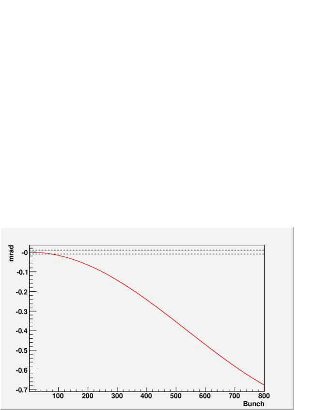
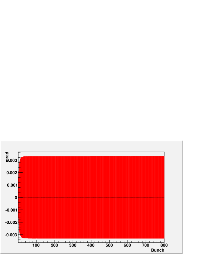
The monopole mode will, with over 800 bunches in the FLASH configuration, take about $800\,\mathrm{k}eV$ out of the last bunch in the train. The maximum of $F_{I}$ corresponds to about $468\,\mathrm{H}z$ from the exact on-resonance condition for all of the dipole modes . The deflection from the dipole mode of highest $\frac{R^{(m)}}{Q}$ in this case is shown in Figure 12; the other modes have the same shape but with the vertical scale proportional to $\frac{R^{(m)}}{Q}$. Figure 13 shows the crabbing angle, defined as the deflection angle (in the lab frame) at the $1\sigma_{z}$ bunch head minus the deflecting angle at the bunch center. This is computed by changing, in effect, the trailing distance of the witness by one bunch-length, and taking the difference in displacement from the centroid displacement.

We do not have a clear understanding as to how this can effect the lasing process, but note that the angles involved are typically smaller than the deflecting angles. The energy loss in this dipole mode at this pseudo-resonance condition is only $5keV$.

It is clear that even a single cavity hitting the worst-case will cause lasing to stop.

Figure 12: Bunch deflection as a function of bunch number, worst case analysis of the $4.834$ GHz mode. For this mode, $Q=5.4\times 10^{9}$, $d=2.77\times 10^{-6}$, and $\widehat{\theta}=1.22$ mrad.

Figure 13: Bunch crabbing as a function of bunch number, worst case analysis of the $4.834$ GHz mode.

4.3 Typical-case analysis, FLASH beamline

In the typical-case analysis we use the Monte Carlo method to examine the probability distribution for beamline performance.

A virtual beamline is constructed of 4 cavities. The frequencies of the modes are shifted from the nominal simulation results of Table 2 by drawing on a uniform random distribution. The width of the distribution spans the full range of $\delta$, corresponding to a frequency shift of $-0.5$ MHz to $+0.5$ MHz in the FLASH case, and 1/5th that for the XFEL injector. While we do not have enough cavities to really check, this is thought to be about the scale on which the scatter will actually be.

Simulated results such as in Figures 12 and 13, along with the corresponding energy loss plot are recorded. Then a new beamline, constructed with new calls to the pseudo-random number generator is created and again, variation of deflection, crabbing, and energy loss with respect to bunch number is determined. The process is repeated 5000 or in some cases, 10000 times. At each bunch number, we have an average and an RMS, over those beamlines, of deflection, crabbing, and energy loss.

The average deflection over an ensemble is easily seen to be zero, as deflection to the left is just as likely as deflection to the right. The average energy loss is also zero; the $\sin$ of Equation 2.2.3b is replaced by the $\cos$ of Equation 2.2.3a. The widths of the distributions of deflection angle, crabbing angle and energy loss describe at the $1\sigma$ level what kind of performance one can expect when the machine is actually turned on.

Clearly, a design that will keep deflection down to our $\pm 10\mu$rad goal at the 68.27% (1$\sigma$) confidence level is risky; we need the RMS to be well below the goal. How far below is a difficult decision involving overall program risk. Notwithstanding, a statistical analysis is able to provide us with a good sense of what levels of external damping we need to have.

Again, we do not obtain an acceptable result on just cavity self-damping alone. If the HOM design fails across the board, deflections of $\sim\pm 50\mu$rad appear at the $1\sigma$ level by the end of an 800 bunch train in the 4 cavity, 5 mode FLASH model, as shown in Figure  14. Next, we determine how far we smust lower $Q_{ext}$ to stabilize the beam.

Figure 14: The one-sigma deflection profile as a function of bunch number, averaged over ensemble of 5000 virtual FLASH beamlines without external dampers.

For the $7.506\,\mathrm{M}Hz$ monopole mode, lowering $Q_{ext}$ to a bit below $1\times 10^{7}$ causes the RMS of $\Delta E$ to flatten out at large bunch numbers to about $23\,\mathrm{k}eV$.

For the dipole modes, there is some allocation of the $\pm 10\mu$rad target into the three modes; we have to also allocate fractions of the deflection budget to the different deflecting modes. If we require that the RMS deflection flattens out to a level where $\pm 10\mu$rad corresponds to $3\sigma$ of the total deflection, and then allocate the deflection budget evenly among our three large dipole modes, then each mode must contribute $10\mu$rad$/(3\sqrt{(}3))=1.9\mu$rad in the asymptotic limit for the 4 cavities, as the contributions from the included modes are added in quadrature.

The Monte Carlo calculation differs from the analytic form of section 3.6.1 in that

1. In the MC method, the asymptotic limit is not assumed. It will in most cases be justified because the damping is strong.

2. In the MC method, angles are summed over modes and cavities, and then an RMS is taken; in the analytic form, the sequence of these two operations is inverted.

3. In the analytic form, the damping constants of all the modes are forced to be equal; in the MC method, the deflection in the long-bunchtrain limit are taken to be equal.

4. Equation 85 sets $10\mu{\rm rad}$ to 1 times the RMS deflection; section 3.6.2 discusses alternate, tighter constraints. The MC method uses a $3\sigma$ constraint.

The Monte Carlo results can be reproduced with analytically. With the required values of $Q_{ext}$, the asymptotic form of Equation 61 permits direct solution for $Q_{ext}$ using the definition of $\widehat{\theta}$ and $d$. These relations lead to $Q_{ext}$ for the 3 modes of $3.7\times 10^{4}$, $2.5\times 10^{5}$ and $1.7\times 10^{5}$, or about 70-80% of the MC values.

The $Q_{ext}$ values that produce deflections of the specified level in the Monte Carlo, found basically by trial and error, are shown in Table 9, along with the results of section 3.6.1 when a $3\sigma$ constraint is used, the results of Phillipe Piot’s (unpublished) calculation and the recent measurements from prototypes [10]. The system is well damped in the simulation, as shown in Figure 15.

Frequency	Azimuthal	$Q_{ext}$
(GHz)	number	MC method	$3\sigma$ Analytic	Piot spec.	Measured
7.506	0	$1.0\times 10^{7}$			$1\times 10^{4}$
4.834	1	$5.4\times 10^{4}$	$9.0\times 10^{4}$	$2.8\times 10^{3}$	$1\times 10^{4}$
5.443	1	$2.9\times 10^{5}$	$1.0\times 10^{5}$	$1.0\times 10^{5}$	$5\times 10^{4}$
7.668	1	$2.1\times 10^{5}$	$1.4\times 10^{5}$	$2.5\times 10^{5}$	$1\times 10^{4}$

Table 9: $Q_{ext}$ requirements from this Monte Carlo study, the analytic forms of 3.6.1 when calculated for a $3\sigma$ constraint, Phillipe Piot’s analysis, and measurement from prototypes. The FLASH beam parameters are used. The value of $d_{rms10}/3$ is 0.169.

Figure 15: The one sigma deflection profile as a function of bunch number, averaged over ensemble of 10000 virtual FLASH beamlines, each consisting of 4 cavities and 5 well-damped modes.

4.4 Typical-case analysis, XFEL injector beamline

The typical-case analysis for our canonical XFEL configuration shows, as expected, that the RMS deflection due to HOMs varies inversely as the beam energy and approximately as the square root of the number of cavities. This makes the deflection about 2/3 of what it would be in FLASH at the same bunch spacing.

Moving the bunch frequency up to $5\,\mathrm{M}Hz$ changes the relative contribution of the dipole modes by changing $d$ and thereby increases the accumulated deflections. Where the asymptotic RMS values of the deflections, scaled to 24 cavities in a $500\,\mathrm{M}eV$ beam would otherwise be $1.2\mu$rad, the introduction of $5\,\mathrm{M}Hz$ bunch frequency results in deflections of about $2.8\mu$rad. To restore $3\sigma$ $10\mu$rad performance, we need the $Q_{ext}$ values of table 10.

Frequency	Azimuthal	$Q_{ext}$
(GHz)	number	MC method	$3\sigma$ Analytic
7.506	0	$1.0\times 10^{7}$
4.834	1	$2.4\times 10^{4}$	$1.8\times 10^{4}$
5.443	1	$1.3\times 10^{5}$	$2.0\times 10^{4}$
7.668	1	$1.0\times 10^{5}$	$2.8\times 10^{4}$

Table 10: $Q_{ext}$ requirements from this Monte Carlo study and the analytic forms of 3.6.1 when calculated for a $3\sigma$ constraint. The XFEL beam parameters are used.

The overall deflection profile still shows a well-damped system; the asymptotic one sigma deflection of $3.39\mu$rad is reached within 60 bunches. The asymptotic energy change is $\sim 58\,\mathrm{k}eV$.

5 Conclusion

We have studied the $Q_{ext}$ requirements for the “third harmonic” cavities using sets of beam parameters typical of FLASH and XFEL operation. A key assumption is that lasing will cease when the deflection due to wakefields approaches the divergence of the beam at the cavity location. We have taken the divergence to be $\pm 10\mu$rad for both beam parameter sets. The XFEL optics in the vicinity of the “third harmonic” cavities is not finalized as we write, but the $\pm 10\mu$rad condition is of the correct scale.

The reader need also be aware of the ’program risk’ issue: what level of statistical confidence that this $\pm 10\mu$rad specification be met without component replacement or change of beam parameters is required? Here, we have selected a $3\sigma$ level of confidence. One might choose to argue that the $3\sigma$ choice is too conservative. Choosing a $1\sigma$ requirement relaxes the damping requirements by about an order of magnitude.

The results are based basically on three modes of high beam-cavity coupling. Adding in quadrature a number of other modes with lower $R^{(1)}/Q$ has little influence ($\sim$25%) on the damping required.

Both analytic and Monte-Carlo based analysis have been done. Both allow for manufacturing defects, but do not allow for the action of any kind of active beam steering system and are quite conservative in that regard.

The results of the two analyses are broadly consistent and are summarized in tables 9 and 10. It is encouraging that the $Q_{ext}$ values measured on prototypes are better than the required values.

For damping values of $Q_{EXT}$ in the $10^{5}$ range, which are typical for functioning HOM mode dampers, the deflections reach their asymptotic values after a few 10’s of bunches. In this case, our analytic results are particularly easy to use, and we summarize them here.

The angular kick on bunch $n\in\{1,2,3\ldots\}$ due to a single mode of angular frequency $\omega$ and quality number $Q$ in a train with bunches $\Delta t$ seconds apart is $\theta_{n}=\widehat{\theta}F_{I}(\delta,d)$ where

$$\widehat{\theta}_{n} = \frac{e\,q_{bunch}}{E_{beam}}\,c\,\frac{R^{(1)}}{Q}\,r_{0}$$

$$\delta = \omega\,\Delta t$$

$$d = \frac{\omega}{2\,Q}\,\Delta t.$$

The function $F_{I}$, which describes the bunch-to-bunch amplification of the wakes, has a maximum at

$$\delta_{\rm max} = \arccos(\frac{1}{\cosh(d)})\approx d-\frac{d^{3}}{6}+\dots$$

$$F_{I}(\delta_{\rm max},d) = \frac{1}{2\,\sinh(d)}$$

and an RMS of

$${\rm RMS}(F_{I}) = \sqrt{\frac{1}{2\pi}\int_{-\pi}^{\pi}d\delta F_{I}(\delta,d)^{2}}$$

$$= \frac{1}{2}\sqrt{(\coth(d)-1)}.$$

6 Acknowledgement

We thank Don Edwards for an illuminating conversation.

References

- [1] R. Wanzenberg, Monopole, Dipole and Quadrupole Passbands of the TESLA 9-cell cavity, TESLA 2001-33, Sept. 2001
- [2] T. Weiland, R. Wanzenberg, Wake fields and impedances, in: Joint US-CERN part. acc. school, Hilton Head Island, SC, USA, 7 - 14 Nov 1990 / Ed. by M Dienes, M Month and S Turner. - Springer, Berlin, 1992- (Lecture notes in physics ; 400) - pp.39-79
- [3] T. Weiland, On the numerical solution of Maxwell’s Equations and Applications in the Field of Accelerator Physics, Part. Acc. 15 (1984), 245-292
- [4] MAFIA Release 4 (V4.021) CST GmbH, Büdinger Str. 2a, 64289 Darmstadt, Germany
- [5] T. Weiland, Comment on wake field computation in time domain, DESY M-83-02, Feb. 1983
- [6] P.B. Wilson High Energy Electron Linacs: Application to Storage Ring RF Systems and Linear Colliders, AIP Conference Proceedings 87, American Institute of Physics, New York (1982),p. 450-563
- [7] W.K.H. Panofsky, W.A. Wenzel, Some considerations concerning the transverse deflection of charged particles in radio-frequency fields , Rev. Sci. Inst. Vol 27, 11 (1956), 967
- [8] W.F.O. Müller, J. Sekutowicz, R. Wanzenberg and T. Weiland, A Design of a 3rd Harmonic Cavity for the TTF 2 Photoinjector, TESLA-FEL 2002-05, July 2002. T. Khabiboulline, N. Solyak and R. Wanzenberg, Higher order modes of a 3rd harmonic cavity with an increased end-cup iris FERMILAB-TM-2210, DESY-TESLA-FEL-2003-01, May 2003.
- [9] M. Abramowitz, I.A. Stegun, (eds.) Handbook of Mathematical Functions, 9th printing, Dover, New York 1970
- [10] T. Khabiboulline, private communication.