The Stonehenge Technique. A new method for aligning coherent bremsstrahlung radiators.

Abstract

This paper describes a new technique for the alignment of crystal radiators used to produce high energy, linearly polarized photons via coherent bremsstrahlung scattering at electron beam facilities. In these experiments the crystal is mounted on a goniometer which is used to adjust its orientation relative to the electron beam. The angles and equations which relate the crystal lattice, goniometer and electron beam direction are presented here, and the method of alignment is illustrated with data taken at MAMI (the Mainz microtron). A practical guide to setting up a coherent bremsstrahlung facility and installing new crystals using this technique is also included.

1 Introduction

In the coherent bremsstrahlung technique a thin crystal oriented correctly in an electron beam can produce photons with a high degree of linear polarization [1]. A typical photon energy spectrum is shown in figure 1, where the region of high polarization is under the peak to the left of the coherent edge whose position depends on the orientation of the crystal relative to the electron beam.

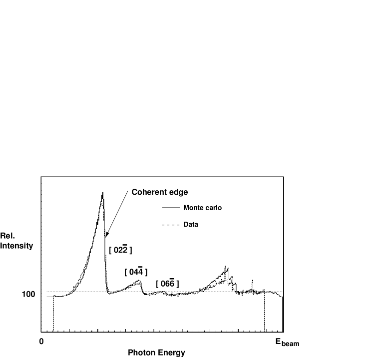
Figure 1: Typical coherent bremsstrahlung enhancement spectrum. The spectrum obtained from the crystal is divided though by a reference spectrum from an amorphous radiator and normalised to be 100 in regions where there is only a small coherent contribution.

The crystal is mounted on a goniometer to control its orientation, but in order to be able to set up coherent bremsstrahlung it is first necessary to measure an appropriate set of angular offsets between the crystal axes and electron beam direction. A method for measuring offsets and aligning the crystal was developed by Lohman et al, and has been used successfully in Mainz [2]. However, recent attempts to investigate new crystals have shown that this approach has limitations which become more serious at higher beam energies where more accurate setting of the crystal angles, which scale with $1/E_{beam}$, is required. (Eg. the recent installation of coherent bremsstrahlung facility at Jlab, with $E_{beam}\simeq$ 6GeV ) This paper describes a new alignment technique which overcomes these limitations. Wherever possible, specific examples are given to illustrate the technique, and section 7 outlines some general methods for installing new crystals and measuring the angular offsets of the electron beam in the goniometer reference frame.

2 Coherent bremsstrahlung - a simplified view.

To provide a linearly polarised photon beam for an experiment we need to be able to adjust the orientation of the polarization plane and the shape of the photon intensity distribution which determines the degree of linear polarization in the photon energy range of interest. The main coherent peak is produced by scattering from one specific set of crystal planes, represented by reciprocal lattice vector g = [$g_{x}g_{y}g_{z}]$. In practice a thin diamond crystal cut in the 100 orientation is used and the main peak is produced by scattering from the set of planes represented by the $[022]$ or $[02\overline{2}]$ reciprocal lattice vector, since this produces the highest polarization. For simplicity, formulae and examples will be presented for these conditions with some remarks on how to generalise to other crystals in different orienations, and different lattice vectors. The parameters of interest are illustrated in figure 2, where the sets of crystal planes defined by the $[022]$ and $[02\overline{2}]$ lattice vectors are represented by 2 orthogonal surfaces.

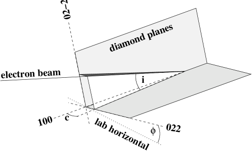
Figure 2: Illustration of the scattering angles for coherent bremsstrahlung from a diamond in the 100 orientation. The sets of planes defined by the $[022]$ and $[02\overline{2}]$ lattice vectors are represented by 2 single orthogonal planes.

The angle of the polarization plane is fixed by $\phi,$ the azimuthal orientation of the 022 axis relative to the lab horizontal, and the position of the main coherent edge (specifically, its fractional energy $x=E_{edge}/E_{beam}$) is controlled by the angle c between the electron beam and the $[02\overline{2}]$ planes. In practice then, c must be adjusted to position the main coherent peak at the region of interest. This will also set the position of subsequent harmonics. For example, in figure 1 the main peak is produced by scattering from the $[02\overline{2}]$ planes and subsequent lower strength peaks from $[04\overline{4}]$ and $[06\overline{6}]$ are also clearly visible; all of these move in-concert as the angle $c$ between the beam and the $[02\overline{2}]$ planes is adjusted. To control the remaining components of the distribution, whilst keeping the main coherent peak (and harmonics) fixed, requires adjustment of the angle $i$ between the electron beam and the direction orthogonal to $c$. This angle will generally be set higher than $c$ by a factor of about 4, to position the coherent contributions from the orthogonal planes at a high photon energy beyond the peak of interest.

Referring to figure 2, we choose the values of $\phi,c,i$ as follows:

1. $\phi$ - the angle between the 022 axis and the horizontal.
   
   This is simply selected by deciding which orientation of the polarization plane is best for the detector geometry of the experiment. Often, for systematics, experiments are run with two orthogonal settings of the polarization plane, $\phi$ and $\phi+\pi/2$. For practical reasons this is most easily achieved by swapping the values of $c$ and $i$, rather than adjusting $\phi$. With $c,i$ as show in figure 2, the polarization plane is $\phi$. Swapping them makes the polarization plane $\phi+\pi/2$. A further common simplification is to use PARA / PERP polarizations, where the polarization plane is parallel or perpendicular to the lab horizontal.
   

2. $c$ - the small angle between the beam and the $[02\overline{2}]$ planes which fixes the position of the coherent edge.
   
   For a diamond in the 100 orientation, if we restrict our interest to the position of the coherent edge from g = $[022]$,$[02\overline{2}]$,$[044]$,$[04\overline{4}]$ etc. then $c$ (in radians) can be calculated as follows:”

   $$c\simeq\frac{k}{gE_{0}^{2}[\frac{1}{E}-\frac{1}{E_{0}}]}$$ (1)

   where:
   $g$= $\pm 2,\pm 4,\pm 6$ ….
   $E$ = required position of coherent edge (MeV)
   $E_{0}$ = electron beam energy (MeV)
   $k=m_{e}a/4\sqrt{2}\pi=$ 26.5601 MeV
   $m_{e}=$ mass of electron = 0.511 MeV
   $a$ = diamond lattice constant = 923.7 (dimensionless units)
   
   In practice, the coherent edge position $E$ should be reasonably close to the calculated value, but this depends on how accurately the initial angular offsets are measured during the setup (see section 7). The position of the coherent edge is tuned by looking at enhancement spectra and making small adjustments to $c$.
   

3. $i$ - the angle between the beam and the orthogonal planes.
   
   This is set to be larger than $c$ by about a factor of 4 and then tuned using feedback from the enhancement spectra. It needs to be adjusted to ensure that the main coherent peak is as clean as possible and that there are no interfering contributions from any higher order lattice vectors.

For the purposes of comparing with bremsstrahlung calculations it is neccessary to describe the orientation in terms of the crystal angles $C_{\theta},C_{\alpha},C_{\phi}$, where $C_{\theta},C_{\alpha}$ are the polar and azimuthal angles of the electron beam in the reference frame of the crystal (defined by the 100, 010, 001 axes) and $C_{\phi}$ is the azimuth of g in the same reference frame. This is represented in figure 3, which is effectively a 2D view of figure 2 looking along the 100 axis. Here, since the polar angles between the beam and crystal are small, $c$ and $i$ are represented by two lines parallel and perpendicular to the 022 axis. This diagram shows that the relationship between $\phi,c,i$ and $C_{\theta},C_{\alpha},C_{\phi}$ is rather simple.

$$C_{\phi}=\frac{\pi}{4}$$ (2)

$$C_{\theta}=\sqrt{c^{2}+i^{2}}$$ (3)

$$C_{\alpha}=C_{\phi}+\tan^{-1}\frac{i}{c}$$ (4)

Figure 3: Diagram showing the relationship between $c,i.\phi$ and crystal angles $C_{\theta},C_{\alpha},C_{\phi}$.

In summary, for a diamond in the 100 orientation with the coherent peak coming from the $[022]$ or $[02\overline{2}]$ planes, we have a simple prescription for deciding on values of $\phi,c,i$. We also have simple set of equations (eq. 2,3,4) for calculating the corresponding angles $C_{\theta},C_{\alpha},C_{\phi}$ in the crystal reference frame; this is important for comaprision with bremsstrahlung calculations. What is also required is a fast, reliable method of setting up and calibrating the goniometer to allow the angles $c,i,\phi$ to be easily selected. A new method for doing this is described in the following sections.

3 Definition of angles and offsets

As shown in Figure 4, the diamond is attached to the inner plate of the goniometer (white circle) which can rotate azimuthally ($\phi$) inside a nested pair of frames which can rotate about vertical and horizontal axes ($v$ and $h$). The curved arrows on the figure indicate the +ve direction of motion on each of the axes. The goniometer should be set up in close alignment with the lab frame and the beam direction. Explicitly, the settings on the $v$ and $h$ axes should be zero (ie the origins defined in the goniometer setup) when these axes are aligned with the lab vertical and horizontal, and the normal to the inner plate O is aligned as closely as possible with the beam direction B. Even with careful initial setup of the goniometer there will be a small, but non-negligible, misalignment with the beam direction B, which may also vary slightly each time new beam is set up for an experiment. There will also be a misalignment of the 100 diamond crystal axis D with the normal to the inner plate O due to imperfections in the mounting and in the cutting from the original stone. These angles are typically in the range 0 - 60mrad, and are highly exaggerated in the diagram for clarity. A simple and direct way of visualising the relative orientation of the beam, goniometer and crystal is to project the vectors B and D onto a 2D plane, where a +ve rotation about the $v$ axis moves D to the right, and +ve rotation about the $h$ axis moves D upwards. The origin of this system is defined by O, the orientation of the normal to the goniometer in its zero position. The azimuthal orientation of the 022 axis relative to the lab horizontal can also be represented on this plot. The D vector sweeps out a cone of angle $\Theta$ when the goniometer is rotated about it’s azimuthal axis.

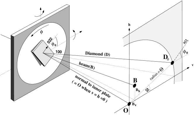
Figure 4: Diamond radiator mounted on a goniometer showing the default angles of the beam (B) and diamond (D), and definitions of angular offsets.

Figure 4 represents the crystal in its default position. Ie. the goniometer has been set up and aligned approximately with the beam direction, and a new crystal has been mounted with the 100 axis also approximately aligned with the beam direction. An appropriate set of angular offsets to describe this are:

• $\phi_{0}$ - the azimuthal offset of the crystal as defined by the angle between the 022 axis and the lab horizontal.

• B_v,B_h - the offsets between the beam direction B and the origin O.

• $\Theta,\Phi$ - the offsets of the 100 axis in the default position D₀, in terms of its polar angular displacement $\Theta$ from the origin O, and the angle $\Phi$ between D₀ and the horizontal.

If these 5 offsets are known then it is possible to position the crystal at any azimuthal angle, with any required small angular orientation of the diamond D relative to the beam B. As described in section 2, the aim is to move the diamond from its default orientation D₀ to some position D_ϕ,c,i where three angles $\phi,c,i$ are set at their required values. The movement from D₀ to D_ϕ,c,i has to be achieved by setting the appropriate angular coordinates on the goniometer’s azimuthal, vertical and horizontal axes $G_{a},G_{v},G_{h}$. The derivation of these coordinates as functions of the angular offsets and desired orientation angles ($\phi,c,i$) is illustrated in figure 5, which shows a graph in angular displacement about the v and h rotation axes.

Figure 5: Angles involved in moving from default position D₀ to an arbitrary position D_ϕ,c,i.

The movement from D₀ to D_ϕ,c,i can be thought of as a 2 step process: Firstly, the crystal needs to be rotated azimuthally by adjusting $G_{a}$ to set the correct orientation $\phi$ of the 022 axis. This has the effect of changing the angular offset between the 100 diamond axis D and the beam B, shown as movement from D₀ to D_ϕ in figure 5. Secondly, the goniometer’s vertical and horizontal rotation coordinates $G_{v},G_{h}$ must be adjusted to set the correct angle between the diamond and the beam. In terms of figure 5 this means a translation from D_ϕ to D_ϕ,c,i.

Applying simple trigonometry to figure 5 gives the following expressions for the goniometer settings $G_{a},G_{v},G_{h}$ required to achieve the diamond orientation D_ϕ,c,i.

$$G_{a}=\phi-\phi_{0}$$ (5)

$$G_{v}=c\cos\phi-i\sin\phi-\Theta\cos(G_{a}+\Phi)+B_{v}$$ (6)

$$G_{h}=c\sin\phi+i\cos\phi-\Theta\sin(G_{a}+\Phi)+B_{h}$$ (7)

Note, this will set the 022 axis at azimuthal angle $\phi$. However, since the crystal has 4 fold symmetry about the 100 axis, interchanging the values of $c$ and $i$ rotates the polarization plane by $\pi/2$, and hence all orientations of the polarization plane are possible with azimuthal rotations of $\leq\pi/4$ relative to the default orientation.

This gives a prescription for selecting the orientation of the polarization plane, and the energy of the coherent edge, provided the offsets $\phi_{0},\Phi,\Theta,B_{v},B_{h}$ are known. The challenge is to find a method of measuring these offsets by scattering electrons from the diamond and interpreting shape of the resulting photon energy spectra. The method described here is the Stonehenge Technique.

4 Lohman’s method and the need to extend it

In the alignment technique developed by Lohman et al [2], angular offsets are measured by carrying out a series of scans, each involving a sequence of small angular movements (steps) of the crystal with the corresponding accumulation of a photon energy spectrum (obtained from a tagging spectrometer). This is divided through by an incoherent spectrum from an amorphous radiator to highlight the coherent contribution and eliminate the effect of channel to channel variations in the rates on the individual counters of the tagging spectrometer. A single slice of such a scan produces an enhancement plot such as that shown in figure 1. The results of the complete scans are plotted on 2d histograms which give information information about the orientation of the crystal. This technique has been very successful, and the method described here can be considered as an extension of it. In summary, Lohman’s technique relies on scans where only a single goniometer coordinate is varied at once. The default azimuthal orientation $\phi_{0}$ is determined by scanning in $G_{a}$. The orientation of the crystal 022 vector is then selected to be $\phi=0^{\circ}$ to allow the orientation of polarization plane to be $0^{\circ}$ or $90^{\circ}$(conventionally PARA or PERP). Once the $G_{a}$ coordinate is fixed for PARA / PERP conditions are considerably simplified since the $[022]$ and $[02\overline{2}]$ reciprocal lattice vectors are now aligned with the v and h axes of the goniometer. Equations 6 and 7 reduce to:

$$G_{v}=c+k_{v}$$ (8)

$$G_{h}=i+k_{h}$$ (9)

Here, $k_{v}$ and $k_{h}$ are the angular offsets beween the beam B and diamond D in this specific PARA / PERP orientation. These offests can be simply determined with scans in $G_{v}$ and $G_{h}$. Once $k_{v}$ and $k_{h}$ have been measured the coherent peak can easily be put at any required energy setting for either PARA or PERP polarization. For brevity only the essential concepts have been described here, the full details are given in Lohman’s paper [2].

Of all the offsets defined in figures 4 and 5, only $\phi_{0}$ is measured explicitly in Lohman’s technique. There is no need to measure the others if we adhere to the special circumstance of only using the PARA / PERP orientations of the crystal. However, setting up for PARA / PERP relies on measuring $\phi_{0}$, by scanning in $G_{a}$. This is non-trivial, since any scan in $G_{a}$ makes the crystal axis D describe a cone in space (see figure 4) and therefore changes 3 parameters simultaneously ($\phi,c,i$). The resulting 2D plot can be difficult (or impossible) to interpret. In practice, the setting up of a new crystal is very time consuming, and relies on the experience and intuition of the user, who has to carry out a series of exploratory and iteratative scans until a consistent picture is obtained. This can only be done reliably if the initial misalignment between the beam B, goniometer O and crystal D is small (ie $\leq$ $1/[2E_{beam}(GeV)]^{\circ}$). A faster, more general technique is described here. This new method is still based the interpretation of scans, but can cope with a larger mounting misalignment and, since it measures all of the offsets described in section 3, allows any arbitrary orientation of the polarization plane to be selected.

5 The Stonehenge Technique

The basis of the stonehenge technique is an hv scan which sweeps the crystal axis D around in a cone of angular radius $\theta_{r}$ by stepping sinusoidally on the $v$ and $h$ axes as follows:

$$\begin{array}[]{c}G_{v}=S_{v}+\theta_{r}\cos\left(\phi_{r}\right)\\ G_{h}=S_{h}+\theta_{r}\sin\left(\phi_{r}\right)\end{array}\left\}\begin{array}[]{c}\end{array}0\leq\phi_{r}<2\pi\right.$$ (10)

where $S_{v},S_{h}$ are the coordinates of the center of the scan relative to the zero positions on the goniometer axes. For each point $G_{v},G_{h}$ in the scan an enhancement spectrum is measured, and, since the intensity is a function of $E_{\gamma,}G_{v},G_{h}$, a full representation of the data can be made by plotting it on surface of a cylinder (figure 6).

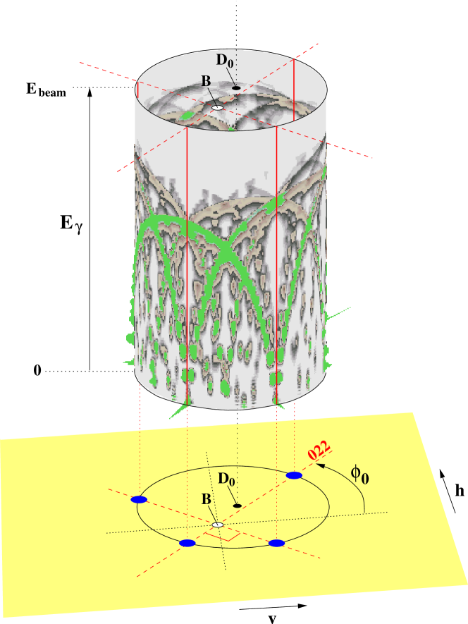
Figure 6: Simulation showing the construction of a stonehenge plot from an hv-scan on a crystal.

Regions of high intensity form sets of curves which show the coherent contributions from different sets of crystal planes as their angles change relative to the beam. The curves with the strongest intensity relate to scattering from the sets of planes defined by the $[022]$ and $[02\overline{2}]$ reciprocal lattice vectors, and the points in the scan where they converge at $E_{\gamma}=0$ indicate where the relevant set of planes is parallel to the beam. Vertical lines are drawn though these 4 points in figure 6 and projected onto the perimeter of a circle to produce a stonehenge plot. By fitting a pair of orthogonal lines to these 4 points the beam position can be identified. The azimuthal offset $\phi_{0}$ of the crystal can be measured, and the offset vector $\overrightarrow{BD_{0}}$ between the crystal axis default position D₀ and the beam direction B determined. Notice that the choice of which of the 2 lines represents the 022 axis is somewhat arbitrary due to the the 4-fold symmetry, so we choose such that $\phi_{0}$ is between 0 and $\pi/2$. For practical reasons the cylinder shown in figure 6 is flattened out onto the outer part a polar diagram with photon energy increasing in the outward radial direction . The stonehenge plot is then constructed in the center. Figures 7 and 8 show the result of such measurements carried out in Mainz using a 100$\mu$m crystal. The 100 axis was made to describe a cone in 180 x 2^∘ steps by moving the goniometer axes as described by eqn. 10, with $\theta_{r}=60$ mrad and $S_{v}=S_{h}=0.$

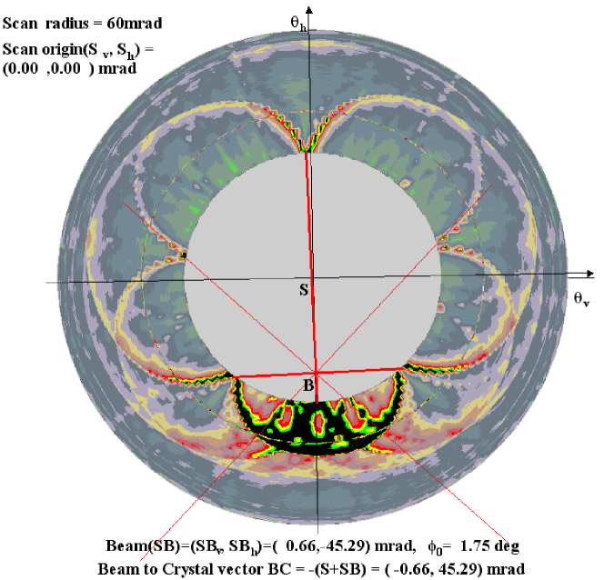
Figure 7: An hv scan and associated stonehenge plot showing calculated offsets for the 100$\mu$m Mainz crystal in the default orientation.

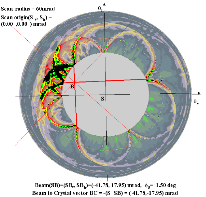
Figure 8: An hv scan and associated stonehenge plot showing calculated offsets for the Mainz 100$\mu$m crystal rotated azimuthally by 180^∘ from the default orientation.

The plotting and analysis was carried out using a ROOT macro [3, 4] which was used to superimpose lines on the polar plot on the basis of 4 selected points (corresponding to the $[022]$ and $[02\overline{2}]$ vectors). This was carried out repeatedly until a pair of orthogonal lines was found to give a good fit to the 4 points (judged by eye). The intersection of these lines defines the coordinates of the beam relative to the center of the scan. Further corroboration that the correct points have been selected is given by the lines at 45^∘ to the main pair, which pass though the points related to the [004] and [040] vectors. The crystal’s azimuthal orientation $\phi_{0}$ is found from the gradient and the vector $\overrightarrow{BD_{0}}$ calculated as follows: $\overrightarrow{BD_{0}}=-(\overrightarrow{S}+\overrightarrow{SB})$, where $\overrightarrow{S}$ ($S_{v},S_{h}$) is the origin of the center of the hv scan in relation to the goniometer origin O. Initially $\overrightarrow{S}$ will be (0,0) but if extra precision is required the scan can be repeated with $\overrightarrow{S}$ set to the first measured value of $\overrightarrow{SB}$ and a smaller radius $\theta_{r}$. Figures 7 and 8 show the output of the ROOT macro with the template correctly fitted and all the values calculated.

Initially the Stonehenge technique seems rather abstract, so it is worth pointing out some of its advantages. A single $hv$-scan with corresponding Stonehenge plot allows the simultaneous measurement of the azimuthal position of the crystal and the vertical and horizontal angles it subtends relative to the beam. With the previous method each of these had to be measured separately through a long process of iterations, with the caveat that the mounting misalignment had to be small. Here, even in conditions where there is a large mounting misalignmet, the scan can be repeated with a large enough radius to produce an unambiguous plot. Also, if only PARA / PERP running conditions are required, the azimuthal orientation is set to $0^{\circ}$ by adjusting $G_{a}$ and the scan repeated to find the offsets $k_{v},k_{h}$ from eq. 8,9 (more details are given in section 7). Furthermore, the speed and reliability of the Stonhenge technique make it practical to measure all of the offsets defined in section 3 and really allows the choice of any arbitrary values of $\phi,c,i$ (see following section). Finally, it is relatively simple to align a crystal with a different structure, or in a different orientation; we just need to calculate which lattice vectors will give the strongest contribution to the coherent bremsstrahlung and overlay a corresponding template on the Stonehenge plot. For example, figure 9 shows the data from a diamond in the 110 orientation after alignment, where the template consists of lines in the 11$\pm 1$, 220 and 004 directions.

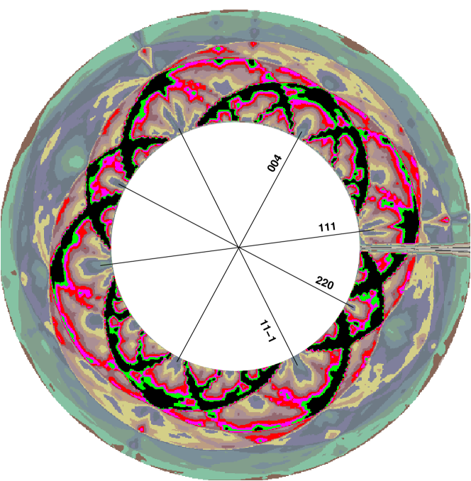
Figure 9: Stonehenge plot of a diamond in the 110 orientation. Here, the crystal was aligned with the beam and the 111 axis set at 10^∘ to the horizontal for measurements of channeling radiation.

6 Obtaining a complete set of offsets from scans

As shown in the previous section, it is possible to measure the azimuthal orientation of the crystal and the offset between the beam B and crystal axis D with a single scan. For many experiments this may provide enough information to run at all the required conditions - eg. only in PARA / PERP mode. However, we can achieve more generality.

We represent the offset between the beam B and crystal axis D with a vector $\overrightarrow{BD_{0}}$, measured from an initial scan. If the goniometer is rotated azimuthally by some known amount $\phi_{s}$, another scan can be carried out to determine a different offset $\overrightarrow{BD_{1}}$ . The vectors $\overrightarrow{BD_{0}}$, $\overrightarrow{BD_{1}}$ with a known angular separation $\phi_{s}$($=\angle D_{0}OD_{1}$) provide the information to locate the origin, construct figure 5 and yield the required offsets. This relationship between $O,\overrightarrow{BD_{0}},\overrightarrow{BD_{1}},\Theta,\Phi$and $\phi_{s}$is shown in figure 10.

Figure 10: Illustration of how to determine derive the offsets $\Phi,\Theta$ and the beam position $B$ from the values of $\overrightarrow{BD_{0}}$ and $\overrightarrow{BD_{1}}$ obtained from two $hv$ scans carried out with an azimuthal separation of $\phi_{s}$.

If the vector components in $v,h$ are $\overrightarrow{BD_{0}}=(v_{0},h_{0})$, $\overrightarrow{BD_{1}}=(v_{1},h_{1})$ then the offsets $B_{v},B_{h},\Theta,\Phi$ are calculated as follows:

$$B_{v}=-\left[\frac{(v_{0}+v_{1})}{2}-\frac{(h_{1}-h_{0})}{2\tan(\phi_{s}/2)}\right]$$ (11)

$$B_{h}=-\left[\frac{(h_{0}+h_{1})}{2}+\frac{(v_{1}-v_{0})}{2\tan(\phi_{s}/2)}\right]$$ (12)

$$\Phi=\arctan\left[\frac{B_{h}+h_{0}}{B_{v}+v_{0}}\right]$$ (13)

$$\Theta=\sqrt{(B_{v}+v_{0})^{2}+(B_{h}+h_{0})^{2}}$$ (14)

In practice, this means carrying out an initial scan to determine $\overrightarrow{BD_{0}}$, rotating by an angle $\phi_{s}$ on the goniometer’s azimuthal axis, and repeating the scan to determine $\overrightarrow{BD_{1}}$. Figures 7 and 8 show the results of such a pair of scans, where the crystal was rotated azimuthally by $\phi_{s}=180^{\circ}$ between scans. As would be expected, the position of the crystal relative to the beam has changed considerably, but both scans agree (to within 0.5^∘) on the azimuthal orientation of the crystal. The components of $\overrightarrow{BD_{0}}$ and $\overrightarrow{BD_{1}}$ obtained from the two corresponding stonehenge plots are inserted into eqns 11-14 to calculate the offsets and construct specific version of the diagram shown in figure 10. The result obtained from the analysis of the 2 example plots (figures 7 and 8) is shown in figure 11, which was generated from a ROOT macro [3, 4].

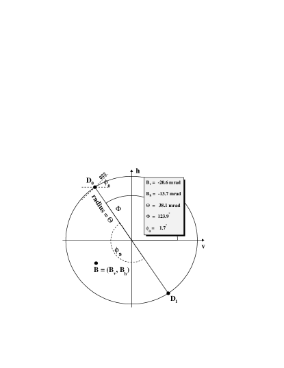
Figure 11: Calculation of the crystal offsets from the results of two hv scans on the Mainz [100]$\mu$m diamond.

With the offsets measured, eqns 5 - 7 can be to used to calculate the goniometer settings required to position the crystal at any desired azimuthal angle ($\phi$) and any desired orientation of the $[022]$ and $[02\overline{2}]$ vectors relative to the beam (ie any values of c and i). To confirm this, we can attempt to set $\phi=0^{\circ}$ , align the crystal perfectly with the beam and carry out another $hv$ scan, which should have symmetry about the $v$ and $h$ axes. An example is shown in figure 12.

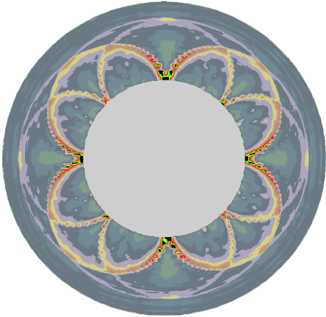
Figure 12: An hv scan of the Mainz $\mu$m crystal in the $\phi_{d}=0$ orientation with all offsets installed (ie center aligned perfectly with the beam).

The Stonehenge Technique has now been used successfully at MAMI in Mainz, CB-ELSA in Bonn, and CLAS at Jefferson Laboratory to align several diamonds. Based on experience at these facilities, the final section is practical, step by step guide on how to setup a linearly polarised photon beam using a combination of the Stonehenge Technique and the methods described by Lohman et al. [2].

7 A step by step guide.

The equations and example plots presented in the earlier sections of this article give a prescription for aligning the crystal relative to the beam for the most general circumstances; ie it is assumed that none of the offsets ($\phi_{0},\Phi,\Theta,B_{v},B_{h}$) are known, and that it is desirable to be able to select any arbitrary orientation of the polarization plane. In practice, this full generality is seldom required. For example, the crystal may have already been installed for an earlier running period, or only the PARA / PERP orientations of the polarization plane may be required. Hence, the steps described below give a suggested procedure for the initial installation and setup of the goniometer, subsequent alignment of new crystals and re-calibration prior to each new run period, and some shortcuts which can be taken for certain specific conditions. It is assumed here that there is a combination of software and hardware in place to move the goniometer in small angular increments and acquire the corresponding photon energy spectra (ie carry out the scans). Several ROOT macros [3] have been developed to carry out the analysis of scans and calculate the goniometer settings. These are available on the web [4], or by sending an email to the author.

Collimation - before and after.

The bremsstrahlung photon beam is tightly collimated to increase the enhancement and the degree of polarization. Ideally it should be collimated to less that half the characteristic angle of the bremsstrahlung cone (eg. 2mm diameter at 23m at CLAS where $E_{beam}\sim 5GeV$). For a true picture of the collimated beam on target, the enhancement needs to be derived from event by event data, where the DAQ is triggered by the photon, and the energy derived by looking at the electron which makes a timing coincidence with the tagger focal plane. Even at a DAQ rate of $\sim 5kHz$ it takes of the order of 30min to build up enough statistics for a reasonable enhancement spectrum. This is certainly useful for measuring the degree of polarization of the beam, but is not adquate for anything requiring fast feedback, such as setup scans, or steering the beam throught the collimator.

The scans described in this paper are based on scalers attached to the tagger focal plane. These count at a high rate (eg $\sim 10^{5}Hz$ per counter) and show the distributions of the scattered bremsstrahlung electrons. They give a very fast enhancement spectrum for the puposes of setup scans, and for setting the coherent edge to the correct position in the photon energy spectrum. The can also provide a fast online monitor that the coherent peak is stable. However, this scaler-derived information does not tell us whether any of the photons made it through the collimator to the experiment.

The distinction between this scaler-based enhancement and a DAQ-based enhancement is important. Just because the coherent peak is in the correct place doesn’t mean the polarized photons are getting through the collimator to the experiment, and there must be adequate other diagnostics in place to ensure that this happens.

Setup of the goniometer

1. The positive directions of rotation of the goniometer should be defined in software to correspond to the directions indicated in figure 4, and the settings on the $v$ and $h$ axes should be zero (ie define $G_{v}=G_{h}=0$) when these axes are aligned with the lab vertical and horizontal, and hence the normal to the inner plate is aligned as closely as possible with the beam direction (generally using a laser and a mirror mounted flat on the plate).

2. Despite the best efforts to setup the goniometer, it is likely that there will still be non-negligible offsets ($B_{v},B_{h}$) between the beam direction and the goniometer. If the beam position is well defined by demanding that it pass through a small collimator, these offsets can be measured during the installation of the first crystal (see below) and used to redefine the zero positions (ie redefine $G_{v}=G_{h}=0$ on the $v$ and $h$ axes of the goniometer. This will mean give a better default alignment between the beam and goniometer.

Reference spectrum

As with the method described by Lohman et al [2], all photon energy spectra obtained with the crystal should be divided though by a reference spectrum obtained with an amorphous radiator, which should be taken immediately prior to attempting to align any crystals. This divides out most of the incoherent bremsstrahlung contribution to the spectrum and highlights the coherent peaks. It also smooths out spikes which are due to the differences in efficiency of the counters to produce a relatively smooth enhancement spectrum. In a highly segmented counter there are likely to be several counters which are dead, or have very low efficiency, and it is recommended that these channels are flagged by entering zeros as appropriate in the reference spectrum. It is then a simple matter to ignore them in the division part of the software and copy the the value from the adjacent (or nearest good) channel. To compare successive steps in the scans it is also necessary to normalize the divided spectra to the same baseline (eg.$\sim 100$). This should be done by multiplying the value in all channels by a normalization factor of [100] $\div$ X, where X is the value of the lowest non-zero channel in the divided spectrum (ie corresponding to a point where there is the smallest possible coherent contribution). This channel will in general be different, and has to be recalculated, for each step in the scan.

Setting up the first crystal

This describes the full alignment procedure on the assumption that all offsets are to be measured, and that is is desireable to be able to dial up any reasonable set of $\phi,c,i$ values. In general only some subset of these steps will be required depending on the required running conditions and on information from any previous alignment.

1. The crystal should be mounted with its face parallel to the goniometer’s inner plate. Experience has shown that is reasonable to expect to mount this to better than 2^∘ (35mrad).

2. An initial hv scan should be carried out (eqn 10) with a radius of $\theta_{r}$ = 60mrad, using 180$\times 2^{\circ}$ steps in $\phi_{r}$, and setting $S_{v}=S_{h}=0$. The resulting data should be used to construct a stonehenge plot as described in section 5, which should give the default azimuthal orientation of the crystal $\phi_{0}$ and the offset between the [100] axis and the beam direction $\overrightarrow{BD_{0}}$. If there is ambiguity in this plot, it is likely to be because the offset between the crystal and the beam is greater than 60mrad and the beam spot lies outside the circle of the stonehenge plot. The scan should be repeated with a greater value of $\theta_{r}$, eg. 120mrad. Once an initial value for $\overrightarrow{BD_{0}}$ has been obtained, it is useful to zoom in and repeat the scan to obtain more accurate value of $\overrightarrow{BD_{0}}$. This is done by setting $\vec{S}=-\overrightarrow{BD_{0}}$ (ie $S_{v}=-v_{0},S_{h}=-h_{0}$) and redoing the original scan with smaller value of $\theta_{r}$. In most situations an initial scan at $\theta_{r}$ = 60mrad, followed by a second scan and $\theta_{r}$ = 20mrad is adequate.

3. The goniometer should be rotated by a known amount $\phi_{s}$ (ideally = 180^∘ if the goniometer and cabling allows), and step 2 repeated. The azimuthal angle measured from the stonehenge plot should be $\phi_{0}$+ $\phi_{s}$, and should yield the same value of $\phi_{0}$ as measured in step 2, to within about 0.5^∘. The second offset between the [100] axis and the beam direction $\overrightarrow{BD_{1}}$ should also obtained from plot.

4. The values of $\overrightarrow{BD_{0}}$ and $\overrightarrow{BD_{1}}$ and $\phi_{s}$ should be used to construct a plot like the one shown in figure 11 and calculate all the offsets ($\phi_{0},\Phi,\Theta,B_{v},B_{h}$)

5. The values of $\phi_{0},\Phi,\Theta$ are specific to this installation of the crystal and should not change unless the crystal is remounted. They should be recorded.

6. The values $B_{v},B_{h}$ describe the offset of the beam. At this point it is sensible redefine the origin of the goniometer to coincide with the beam. Ie. move the goniometer to $G_{v}=B_{v}$ and $G_{h}=B_{h}$ and redefine the zero positions in the goniometer software at these positions. The default values of the beam offsets can now be set to zero ($B_{v}=B_{h}=0$) and should only change if the beam position changes or the goniometer is re-installed.

7. To confirm that the offsets have been correctly measured a final $hv$ scan should be carried out with the crystal in the required azimuthal setting (say $\phi=0$), and the center of rotation aligned with the beam. Setting $\phi=i=c=0$ in eqns 5-7 gives the coordinates $G_{\phi},G_{v},G_{h}$ for the center of scan ($S_{v},S_{h})$.

Installation of other crystals

Other crystals should be aligned in a similar way to the first crystal but with step 6 omitted since the goniometer’s zero setting should now be consistent with the beam direction. Scans on new crystals should confirm the beam position, which should be very close to the origin.

Setting the polarization plane

Since there is 4-fold rotational symmetry about the azimuthal axis, the goniometer need never be rotated by more than $\pm 45^{\circ}$ to position the crystal lattice for any required orientation of the polarization plane. For example, if we select $\phi=30^{\circ}$ (the azimuthal angle of the $022$ crystal axis from the horizontal) and select $c$ and $i$ to be the scattering angles from the $02\overline{2}$ and $022$ axes respectively, as shown in figure 4c, then the polarization plane with be at 30^∘. Interchanging $c$ and $i$ will rotate the plane by 90^∘ to 120^∘ (or -60^∘). Eqn 5 should be used to find the goniometer value $G_{\phi}$ to set the correct azimuthal orientation of the crystal.

Calibrating the crystal.

Once the required azimuthal angle $\phi$ has been set and the required orientation of the polarization plane chosen ($\phi_{pol}=\phi$ or $\phi_{pol}=\phi\pm 90^{\circ}$ ), an energy calibration scan should be carried out to produce a table of goniometer angles vs. coherent edge. This involves fixing the incoherent scattering angle $i$ and stepping through a range of coherent angles $c$. For example, in Mainz where $E_{beam}=855MeV$, the incoherent scattering angle $i$ is set to 60mrad and a typical energy scan would be from -1mrad to +10mrad in steps of 0.25mrad in $c$. In the simplest situation, where the polarization plane is vertical or horizontal, it requires motion on only a single axis, $v$ or $h$, and is described in Lohman’s paper [2]. However, in the more general situation keeping $i$ fixed and stepping in $c$ requires movements on both the $v$ and $h$ axes. Here eqns 5-7 can be used to generate a table of the goniometer settings $G_{v},G_{h}$ corresponding to each $c$ value in the scan. The goniometer settings $G_{v},G_{h}$ required to set the position of the coherent edge to the required photon energy are found by interpolating between the closest points in the table. It is worth stressing here that this calibration is appropriate only for the selected value of the polarization plane $\phi_{pol}$. If this changes, then a new calibration run must be made.

Re-tuning and re-calibrating

If the position of the coherent peak drifts by a small amount during running (eg. due to drift in the beam position) it can be compensated for by making small adjustments to $c$, which in general means adjusting the values to both the $G_{v}$, $G_{h}$ settings, again by interpolation in the calibration table. If there is a large drift in the coherent peak position then it is worth carrying out an hv scan with $\phi$ remaining in its current position and the center $S_{v},S_{h}$ corresponding to $c=i=0$ (see eqns 6,7). The resulting stonehenge plot should confirm the value of the current azimuthal orientation $\phi$, but should be give a non-zero value for $\overrightarrow{SB}$; ie beam position should be offset from the center of the scan. Note that on this information alone it is not possible to say whether the crystal has moved in some way (eg. a from expansion of a mounting wire) or the beam position has changed. However, provided we want to keep the current azimuthal orientation of the crystal $\phi$, this is not important. The components of $\overrightarrow{SB}$ (labeled $SB_{v},SB_{h}$ in figures 7 and 8) can be added to the current beam offsets $B_{v},B_{h}$ and the calibration scan described above can be repeated.

Shortcuts

A single azimuthal orientation.

In many experimental situations it is only necessary to select a single azimuthal orientation $\phi$ of the crystal and to set the polarization plane. This will then be used for one specific orientation of the polarization plane, or for the pair of orthogonal settings which are parallel and perpendicular to this direction ( ie setting $\phi_{para}=\phi$ and $\phi_{perp}=\phi+90^{\circ}$ and interchanging the coherent and incoherent angles $c,i$ ). Here, once the default azimuthal orientation of the crystal $\phi_{0}$ has been determined, the desired azimuthal orientation $\phi$ can be set, and the offset between the beam B and crystal axis D measured specifically for this value of $\phi$. This is achieved by carrying out a procedure similar to that outlined as the first step for installing the first crystal. However, as soon as the default azimuthal orientation $\phi_{0}$ of the crystal is found with adequate precision, the goniometer setting $G_{a}$ should be adjusted to set the crystal to the desired azimuthal orientation ($G_{a}=\phi-\phi_{0}$). The hv scan should then be repeated in this new azimuthal orientation and the value of $\overrightarrow{BD_{0}}(v_{0},h_{0})$ found using the stonehenge plot. The beam offsets are now $B_{v}=-v_{0}$ and $B_{h}=-h_{0}$, and eqns 6 and 7 simplified as follows:

$$G_{v}=c\cos\phi-i\sin\phi+B_{v}$$ (15)

$$G_{h}=c\sin\phi+i\cos\phi+B_{h}$$ (16)

The crystal can now be calibrated as described above, this time using eqns 15 and 16 to generate a series of goniometer settings for a scan in $c$ at a polarization plane of $\phi_{pol}=\phi$. Again, interchanging $c$ and $i$ in eqns 15 and 16 will give the appropriate values for the $\phi_{pol}=\phi+90^{\circ}$.

PARA and PERP

Notice, that if the PARA / PERP settings are being used (ie $\phi=0^{\circ}$ or $\phi=90^{\circ}$) eqns 15 and 16 become simplified further and $c,i$ are related independently to $G_{{}_{V}},G_{h}$.

8 Conclusions

A new method of aligning crystals for coherent bremstrahlung facilities has been described. As with previous methods it still based the interpretation of scans, but can cope with a relatively large mounting misalignment and allows any arbitrary orientation of the polarization plane to be selected. The technique has now become the standard method used for setting up coherent bremsstrahlung at the several of world’s main coherent bremsstrahlung facilities (MAMI at Mainz, CLAS at Jefferson Lab, ELSA at Bonn and MAXLab at Lunz).

The work presented here was funded by the Engineering and Physical Sciences Research Council (EPSRC) and by Eurotag, a Joint Research Activity within the Eurpean Framework 6 I3HP initiative.

References

- [1] Timm U 1969 Fortschritte der Physik. 17 65.
- [2] Lohman D, Schumacher M et al. 1994 Nucl. Instr. and Meth. A 343 494
- [3] Brun R, Rademakers F. ROOT 1996 Nucl. Inst. & Meth. in Phys. Res. A 389 81 See also http://root.cern.ch/.
- [4] http://nuclear.gla.ac.uk/~kl/Eurotag/Software/CoherentBrem
- [5] Natter F, Grabmayr P, Hehl T, Owens R and Wunderlich S 2003 Nucl. Instr. Meth. B 211 465