Dynamical correlations in the Sherrington-Kirkpatrick model in a transverse field

Abstract

We calculate the real-time-correlation function of the Sherrington-Kirkpatrick spin-glass model in a transverse field. Using a careful analysis of the perturbative expansion of the functional-integral representation, we derive the asymptotic form of the correlation function. In contrast to the previous works, we find for large transverse field a power-law decay of the correlation with time $t$ as $t^{-3/2}$ at zero temperature and $t^{-2}$ at infinite temperature. At the small field region, we also find a significant change in the correlation which comes from the structural difference between two paramagnetic phases.

I Introduction

Among disordered systems, spin glasses MPV are of great interest and have been investigated over decades because of the simplicity of the models, the rich resulting properties, and a large amount of applications to a variety of problems such as neural networks and information processing. Nishimori The Sherrington-Kirkpatrick (SK) model SK is one of the objectives which has been intensively investigated and is also known as the most successful example which yields a large number of notable consequences by mean-field approach.

Quantum random magnets are also the objectives of challenge and of significance due to their relevance to the physics of real disordered magnetic compounds at low temperature. However there is an obstacle. Combination of randomness and quantum fluctuation makes the analytical approach complicated. Physically it is expected that spin-glass state may be disturbed by quantum fluctuations at low temperature and the system exhibits quantum phase transitions, which was discussed in several former works. BM ; CDS ; Sachdev

In this paper we single out the SK model in a transverse field among a variety of quantum random magnet models because this is the simplest quantum model exhibiting the spin-glass phase transition and is believed to have direct relationship with the physics of a real disordered compound ${\rm LiHo}_{x}{\rm Y}_{1-x}{\rm F}_{4}$. We concentrate on clarifying the role of the quantum fluctuations for spin-glass systems similar to former works. We use the path-integral formalism for dealing with the quantum fluctuation. The effect of quantum fluctuation can be incorporated as (imaginary) time-dependent order parameters. In Ref. KT, , one of the authors proposed a method for treating such fluctuation effect, where the time dependence of the order parameters is integrated out for deriving a renormalized effective free energy expressed in terms of classically defined time-independent order parameters. This approach is sufficient for extracting static properties of the system, e.g., the phase diagram or time-independent quantities, which can be assessed by the resulting effective free energy. However in this paper we look closely at the time dependence of the order parameter to investigate the dynamical properties of the system. Therefore we resort to another approach to assess time-dependent quantities.

We analyze the local dynamical correlation function at an arbitrary temperature $T=1/\beta$, which is defined as

$$\chi(t)=\left[\frac{1}{Z}\mbox{Tr}\,e^{-\beta\hat{H}}e^{i\hat{H}t}\sigma^{z}_{i}e^{-i\hat{H}t}\sigma^{z}_{i}\right],$$ (1)

where $\sigma^{z}_{i}$ is the $z$ component Pauli-spin operator on site $i$ and $Z=\mbox{Tr}\,\exp(-\beta\hat{H})$ is the partition function with a Hamiltonian $\hat{H}$. In the analysis of quantum systems, the calculation of the dynamical correlation functions is one of the main topics and a variety of analytical techniques have been developed for it. Sachdev ; GKKR As stated above, we consider the SK model in a transverse field $\Gamma$,

$$\hat{H}=-\frac{1}{2}\sum_{i,j=1}^{N}J_{ij}\sigma^{z}_{i}\sigma^{z}_{j}-\Gamma\sum_{i=1}^{N}\sigma^{x}_{i},$$ (2)

where the averaging of the spin coupling $J_{ij}$, denoted by the square brackets in Eq.(1), is taken with the Gaussian distribution.

With regard to the behavior of dynamical correlation function there are many preceding analytical MH ; YSR ; RG ; GR and numerical ARi ; AR works, where Eq.(1) with imaginary time $t=-i\tau$ is analyzed. Their analytical results show that the correlation decays asymptotically as power law of $\tau^{-2}$ at the zero-temperature critical point. Furthermore the authors of Refs. RG, and GR, pointed out the relevance of $\tau^{-2}$ decay to the same behavior of time-correlation function in the single-impurity Kondo model Kondo by making use of the mapping between two models, which seems to enforce the validity of their result. However, the numerical calculation in Ref. ARi, indicates a somewhat smaller value for the power-law index and some argument is required for the discrepancy. All of the former analytical results are based on perturbative expansion, and in this paper we reexamine this calculation by using a careful analysis of the expansion. We arrive at a different conclusion for the value of the power index, which stems from how to deal with multipoint correlation function appearing in the form of expansion.

The paper is organized as follows. In Sec. II, we calculate the imaginary-time-correlation function at zero temperature by using the perturbative expansion. By referring to the diagrammatic expansion method utilized for other quantum systems, we calculate the asymptotic form of the correlation function and make the comparison of it with the known results. In addition the result is confirmed by the numerical calculation. In Sec. III we move on to the correlation at finite temperature. We investigate it numerically and give some considerations to the result, which suggest different asymptotic behaviors of the correlation at high-temperature region from the case of zero temperature. Section IV is devoted to conclusions.

II Correlations at zero temperature

II.1 Imaginary-time formalism

The real-time correlation (1) is obtained by the analytic continuation of the imaginary-time-correlation function,

$$\chi(\tau)=\left[\frac{1}{Z}\mbox{Tr}\,e^{-(\beta-\tau)\hat{H}}\sigma^{z}_{i}e^{-\tau\hat{H}}\sigma^{z}_{i}\right].$$ (3)

The time-independent static part of $\chi(\tau)$, $\chi=\int_{0}^{\beta}d\tau\chi(\tau)/\beta$, was studied in detail in Ref. KT, as a measure of quantum fluctuations. In order to deal with quantum operators analytically, we use the imaginary-time path-integral representation. Following the standard technique we introduce replica to perform the ensemble average. The correlation function is expressed with the path integral of normalized vector,

$$\chi(\tau) = \lim_{n\to 0}\left[\mbox{Tr}\,\exp\left(-\beta\sum_{\alpha=1}^{n}\hat{H}^{(\alpha)}\right)\sigma^{(1)}_{zi}(\tau)\sigma^{(1)}_{zi}(0)\right]$$ (4)

$$= \lim_{n\to 0}\left[\int{\cal D}{\mbox{\boldmath{$s$}}}\,s^{(1)}_{zi}(\tau)s^{(1)}_{zi}(0)\exp\left(\sum_{\alpha=1}^{n}\int_{0}^{\beta}d\tau^{\prime}\left\{i\Phi[\mbox{\boldmath{$s$}}^{(\alpha)}(\tau^{\prime})]-H[\mbox{\boldmath{$s$}}^{(\alpha)}(\tau^{\prime})]\right\}\right)\right],$$ (5)

where the superscript $\alpha$ is the replica index running from 1 to $n$, and the limit $n\to 0$ is taken afterward. $s$ is the unit vector on the Bloch sphere and $\Phi$ is the Berry phase term. Then we put the Hamiltonian of the transverse SK model (2) into the above formula and take the Gaussian average with respect to the interaction $J_{ij}$. After performing the Hubbard-Stratonovich transformation, we have the path integral form of one-body Hamiltonian,

$$\chi(\tau)=\left<s^{(1)}_{z}(\tau)s^{(1)}_{z}(0)\exp\left\{\frac{J^{2}}{2}\sum_{\alpha=1}^{n}\int_{0}^{\beta}d\tau_{1}\int_{0}^{\beta}d\tau_{2}\,s_{z}^{(\alpha)}(\tau_{1})\chi(\tau_{1}-\tau_{2})s_{z}^{(\alpha)}(\tau_{2})\right\}\right>_{\Gamma},$$ (6)

where the angular bracket denotes the path integral over $\mbox{\boldmath{$s$}}^{(\alpha)}(\tau)$ as

$$\langle\cdots\rangle_{\Gamma}=\lim_{n\to 0}\int{\cal D}\mbox{\boldmath{$s$}}\left(\cdots\right)\exp\left(\sum_{\alpha=1}^{n}\int_{0}^{\beta}d\tau^{\prime}\left\{i\Phi[\mbox{\boldmath{$s$}}^{(\alpha)}(\tau^{\prime})]+\Gamma s_{x}^{(\alpha)}(\tau^{\prime})\right\}\right).$$ (7)

The Hubbard-Stratonovich field $\chi(\tau_{1}-\tau_{2})\sim\langle s_{z}^{(\alpha)}(\tau_{1})s_{z}^{(\alpha)}(\tau_{2})\rangle$ is nothing but the time-correlation function (3) and is taken to be free from the replica index. Here we neglect the time correlation between different replicas, or in other words time-dependent spin-glass parameter $q^{\alpha\alpha^{\prime}}(\tau_{1},\tau_{2})\sim\langle s_{z}^{(\alpha)}(\tau_{1})s_{z}^{(\alpha^{\prime})}(\tau_{2})\rangle$ $(\alpha\neq\alpha^{\prime})$ is taken to be zero, which means we are in paramagnetic phase. Our goal is to solve this self-consistent equation for $\chi(\tau)$.

II.2 Self-consistent equation in linear order

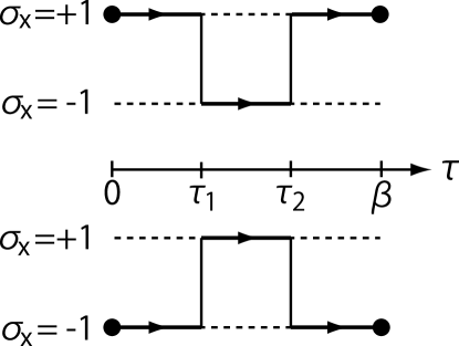
Figure 1: The pictorial representation of the two-point correlation function $D_{\Gamma}(\tau_{2}-\tau_{1})=\langle s_{z}(\tau_{2})s_{z}(\tau_{1})\rangle_{\Gamma}$ with $\tau_{2}>\tau_{1}$.

We expand Eq.(6) as a power series of $J^{2}$ in order to perform the spin integration afterward. Up to the first order, we find the self-consistent linear equation for $\chi(\tau)$,

$$\chi(\tau)=D_{\Gamma}(\tau)+\frac{J^{2}}{2}\int_{0}^{\beta}d\tau_{1}\int_{0}^{\beta}d\tau_{2}\left\{D_{\Gamma}(\tau,\tau_{1},\tau_{2},0)-D_{\Gamma}(\tau)D_{\Gamma}(|\tau_{1}-\tau_{2}|)\right\}\chi(\tau_{1}-\tau_{2}),$$ (8)

where the two-point correlation function $D_{\Gamma}(|\tau_{1}-\tau_{2}|)=\langle s_{z}^{(1)}(\tau_{1})s_{z}^{(1)}(\tau_{2})\rangle_{\Gamma}$ is given by

$$D_{\Gamma}(|\tau_{1}-\tau_{2}|)=\frac{e^{\beta\Gamma-2\Gamma|\tau_{1}-\tau_{2}|}+e^{-\beta\Gamma+2\Gamma|\tau_{1}-\tau_{2}|}}{e^{\beta\Gamma}+e^{-\beta\Gamma}}.$$ (9)

We can easily find how two $s_{z}$’s contribute to this propagator by drawing pictorial spin-flip representation as in Fig. 1. The spin pointing along the $x$ direction is flipped two times by the spin operator $\sigma_{z}$ while propagating from $\tau=0$ to $\tau=\beta$. It is necessary to go back to the original state due to the boundary condition $\mbox{\boldmath{$s$}}(0)=\mbox{\boldmath{$s$}}(\beta)$. KT In the same way, for the four-point function $D_{\Gamma}(\tau_{1},\tau_{2},\tau_{3},\tau_{4})=\langle s_{z}^{(1)}(\tau_{1})s_{z}^{(1)}(\tau_{2})s_{z}^{(1)}(\tau_{3})s_{z}^{(1)}(\tau_{4})\rangle_{\Gamma}$, the spin is flipped four times and we obtain

$$D_{\Gamma}(\tau_{1},\tau_{2},\tau_{3},\tau_{4})=D_{\Gamma}(\tau_{1}-\tau_{2}+\tau_{3}-\tau_{4}),$$ (10)

where we assume $\tau_{1}>\tau_{2}>\tau_{3}>\tau_{4}$. As we see from Fig. 1, it is important to take notice of the time ordering of the spin operators.

The integral equation (8) can be solved by the differential equation for $\chi(\tau)$,

$$\partial_{\tau}^{4}\chi(\tau)-8\Gamma^{2}\partial_{\tau}^{2}\chi(\tau)+16(\Gamma^{4}-\Gamma^{2}J^{2})\chi(\tau)=0,$$ (11)

which is obtained by taking derivatives of Eq.(8) several times and constructing the closed-form equation in terms of $\chi(\tau)$. With the boundary condition it can be solved as

$$\chi(\tau)=\frac{1}{2}\left[D_{\Gamma_{+}}(\tau)+D_{\Gamma_{-}}(\tau)\right],$$ (12)

where $\Gamma_{\pm}=\sqrt{\Gamma^{2}\pm\Gamma J}$. At the zero-temperature limit, this function goes to

$$\chi(\tau)\to\frac{1}{2}\left(e^{-2\Gamma_{+}\tau}+e^{-2\Gamma_{-}\tau}\right),$$ (13)

where we assume $\tau<\beta/2$ in taking the limit $\beta\to\infty$. This result shows that, due to disorder, the energy level splits into two as $\Gamma\to\sqrt{\Gamma^{2}\pm\Gamma J}$. Proceeding further to the higher order correlations, we expect energy levels split into many and finally form a broad distribution, as we see in the following.

However, we must note that this interpretation is valid only when $\Gamma>J$. Solution (12) changes its behavior in the case of smaller transverse fields, which is attributed to the phase transition between the paramagnetic and the spin-glass phases. MH When $\Gamma<J$, the time-independent part $\chi=\int_{0}^{\beta}d\tau\chi(\tau)/\beta$ is nonzero even at zero temperature and nonperturbative analysis is required for the zero mode. KT This sharp change in behavior could be an artifact of the perturbative expansion. Although this change survives even if we take the higher-order correlations into account as we show in the following, it is not clear whether it corresponds to the phase-transition point or not. For example, in the random energy model REM the corresponding phase transition is of first order and it is not possible to determine the transition point from perturbative calculation (see Sec. III.3 for detailed calculations). In the present analytical calculation, we assume that $\Gamma$ is large enough such that the zero mode gives no contribution. Then the correlation asymptotically decays to zero in time and the perturbative expansion is justified. The behavior at small $\Gamma$ is analyzed numerically in Sec. II.5.

II.3 Asymptotic behavior at zero temperature

We take higher-order correlations into account in the following. In general $\chi(\tau)$ including all of such corrections is not tractable, but in the case of the zero-temperature limit the evaluation turns out to be considerably simpler. The integral in Eq.(8) consists of contributions from (i) $\tau_{1,2}<\tau$, (ii) $\tau_{1,2}>\tau$, and (iii) $\tau_{1}<\tau<\tau_{2}$ or $\tau_{2}<\tau<\tau_{1}$. As we found above, the first-order result (13) is short range and decays exponentially with respect to $\tau$. Then we expect that the asymptotic form of $\chi(\tau)$ is dominated by contributions from (i) and (ii) since the constraint in (iii), $\tau_{1}\sim\tau_{2}\sim\tau$, is harder than that in (i) and (ii), $\tau_{1}\sim\tau_{2}$, in performing double integral, which makes the contribution from (iii) negligible. At the limit $T=0$, the contribution from (i) is written as

$$J^{2}\int_{0}^{\tau}d\tau_{1}\int_{0}^{\tau_{1}}d\tau_{2}\left[g(\tau-\tau_{1})\chi(\tau_{1}-\tau_{2})g(\tau_{2})-g(\tau-\tau_{2})\chi(\tau_{1}-\tau_{2})g(\tau_{1})\right],$$ (14)

where $g(\tau)=\exp(-2\Gamma\tau)$. Similarly the contribution from (ii) is given by

$$J^{2}\int_{\tau}^{\beta}d\tau_{2}\int_{\tau_{2}}^{\beta}d\tau_{1}\left[g(\beta-\tau_{1})\chi(\tau_{1}-\tau_{2})g(\tau_{2}-\tau)-g(\beta-\tau_{2})\chi(\tau_{1}-\tau_{2})g(\tau_{1}-\tau)\right].$$ (15)

Using the relation $\chi(\tau)=\chi(\beta-\tau)$, we find that Eq.(15) is given by Eq.(14) with the replacement $\tau$ by $\beta-\tau$. Comparing each term in above two equations we arrive at the conclusion that the main contribution comes from the first term in Eq.(14). We have an approximated form now,

$$\chi(\tau)\sim g(\tau)+J^{2}\int_{0}^{\tau}d\tau_{1}\int_{0}^{\tau_{1}}d\tau_{2}g(\tau-\tau_{1})\chi(\tau_{1}-\tau_{2})g(\tau_{2}).$$ (16)

This equation is solved as

$$\chi(\tau)=\frac{1}{2}\left[e^{-2(\Gamma+J/2)\tau}+e^{-2(\Gamma-J/2)\tau}\right],$$ (17)

which is a good approximation for Eq.(13) when $\Gamma\gg J$.

Higher-order contributions can be incorporated in the same way. We find

$$\chi=g+J^{2}g*\chi*g+J^{4}g*\chi*g*\chi*g+\cdots=\frac{1}{1-J^{2}g*\chi}*g,$$ (18)

where the asterisk $*$ represents a time integral in convolution form,

$$f*g(\tau)=\int^{\tau}_{0}d\tau^{\prime}f(\tau-\tau^{\prime})g(\tau^{\prime}).$$ (19)

This function product satisfies commutativity $f*g=g*f$ and can be treated similar to ordinary product. Solving Eq.(18) we obtain

$$\chi=\frac{1}{2J^{2}g}\left(1-\sqrt{1-4J^{2}g^{2}}\right)=\sum_{n=0}^{\infty}\frac{(2n-1)!!}{(2n+2)!!}2^{2n+1}J^{2n}g^{2n+1},$$ (20)

where we omitted the asterisk $*$. Using the $n$th convolution product of $g$ given by

$$g^{n}(\tau)=\frac{\tau^{n-1}}{(n-1)!}e^{-2\Gamma\tau},$$ (21)

we obtain the result for the imaginary correlation function at zero temperature,

$$\chi(\tau)=\frac{1}{J\tau}I_{1}(2J\tau)e^{-2\Gamma\tau},$$ (22)

where $I_{1}$ is the modified Bessel function of order 1. This function has an asymptotic form of exponential decay,

$$\chi(\tau)\sim\frac{1}{\sqrt{4\pi}(J\tau)^{3/2}}e^{-2(\Gamma-J)\tau},$$ (23)

at $\Gamma>J$, which changes to a power decay $\tau^{-3/2}$ at $\Gamma=J$.

The analytic continuation to the real time is obtained as

$$\chi(t)=\frac{1}{Jt}J_{1}(2Jt)e^{-2i\Gamma t},$$ (24)

where $J_{1}$ is the Bessel function of order 1. This shows $t^{-3/2}$ decay for arbitrary $\Gamma$ as

$$\chi(t)\sim\frac{1}{\sqrt{\pi}(Jt)^{3/2}}e^{-2i\Gamma t}\cos\left(2Jt-\frac{3\pi}{4}\right).$$ (25)

In the Fourier-transformed space, the spectrum forms a semicircle with the center $\omega=2\Gamma$ as

$$\chi(\omega)=\frac{\sqrt{4J^{2}-(\omega-2\Gamma)^{2}}}{J^{2}}\theta(2J-|\omega-2\Gamma|).$$ (26)

It is worth stressing here that the real-time correlation always shows a power-law asymptotic decay (25), while the imaginary-time correlation (23) exhibits a power-law behavior only at $\Gamma=J$. However, as we explained in Sec. II.2, we must be careful about identifying the point $\Gamma=J$ as a critical one. Actually, it is known by preceding works KT ; MH ; AR that the value of $\Gamma$ at the critical point should be a larger one $\Gamma\sim 1.5J$. In order to observe the power-law decay numerically in imaginary-time framework, we must identify the critical point, which turns out to be a troublesome task. ARi On the other hand, in the real-time framework the power-law behavior can be observed not only in the critical point but also in a broad range of large $\Gamma$ where our perturbative calculation is justified. Therefore, we can check the universal power-law index of 3/2 in the paramagnetic phase at zero temperature by observing the semicircle form of the spectrum.

II.4 Comparison with previous results

Our result shows that the correlation decays in power as $t^{-3/2}$. On the other hand, the authors of Ref. MH, have the conclusion of $t^{-2}$ decay via a rather general argument. Their argument is based on a perturbative expansion as we did in the present paper. Actually we obtained the same form (20) as theirs, though there is a minor but crucial difference. The difference originates from the evaluation of the $n$-point correlations with $n\geq 4$. For example, let us recall that we have the four-point correlation $D_{\Gamma}(\tau_{1},\tau_{2},\tau_{3},\tau_{4})=\langle s_{z}^{(1)}(\tau_{1})s_{z}^{(1)}(\tau_{2})s_{z}^{(1)}(\tau_{3})s_{z}^{(1)}(\tau_{4})\rangle_{\Gamma}$ obtained in Eq.(10). In the previous works, MH ; YSR ; RG ; GR the Wick theorem,

$$D_{\Gamma}(\tau_{1},\tau_{2},\tau_{3},\tau_{4})\to D_{\Gamma}(|\tau_{1}-\tau_{2}|)D_{\Gamma}(|\tau_{3}-\tau_{4}|)+D_{\Gamma}(|\tau_{1}-\tau_{3}|)D_{\Gamma}(|\tau_{2}-\tau_{4}|)+D_{\Gamma}(|\tau_{1}-\tau_{4}|)D_{\Gamma}(|\tau_{2}-\tau_{3}|),$$ (27)

was applied to the evaluation of this four-point correlation. However, this expression is not compatible with the exact one (10). It is evident that the integration of the spin variable is not a Gaussian one, and accordingly Eq.(27) is not justified. In order to show that the use of the Wick theorem leads to a wrong result, we examine the self-consistent equation in linear order (8). In our approach we have the solution as Eq.(12), and we should recall that the form of four-point correlation in Eq.(10) was used there. On the other hand, let us suppose that factorization (27) by two-point correlation is correct. Then we can perform the Fourier transformation of $\chi(\tau)$ to find

$$\chi(\omega_{n}=2\pi n/\beta)=D_{\Gamma}(\omega_{n})+\beta^{2}J^{2}D_{\Gamma}^{2}(\omega_{n})\chi(\omega_{n})=\frac{D_{\Gamma}(\omega_{n})}{1-\beta^{2}J^{2}D_{\Gamma}^{2}(\omega_{n})},$$ (28)

where $n$ is an integer and

$$D_{\Gamma}(\omega_{n})=\frac{\tanh\beta\Gamma}{\beta\Gamma}\frac{(\beta\Gamma)^{2}}{(\beta\Gamma)^{2}+(\pi n)^{2}}.$$ (29)

Performing the Fourier transformation again for going back to the imaginary-time representation, we obtain

$$\chi(\tau)=\frac{1}{2}\left[\frac{\Gamma\tanh\beta\Gamma}{\tilde{\Gamma}_{+}\tanh\beta\tilde{\Gamma}_{+}}D_{\tilde{\Gamma}_{+}}(\tau)+\frac{\Gamma\tanh\beta\Gamma}{\tilde{\Gamma}_{-}\tanh\beta\tilde{\Gamma}_{-}}D_{\tilde{\Gamma}_{-}}(\tau)\right],$$ (30)

where $\tilde{\Gamma}_{\pm}=\sqrt{\Gamma^{2}\pm\Gamma J\tanh\beta\Gamma}$. This does not coincide with the exact result (12), which indicates that factorization (27) is not valid. In addition, Eq.(30) does not satisfy the normalization condition $\chi(\tau=0)=1$. The authors of Refs. MH, ; YSR, ; RG, ; GR, introduced a Lagrange multiplier to cure this defect. However, we can show that the correct result is not reproduced even if the Lagrange multiplier is introduced. Consequently we conclude that the factorization is not a correct procedure in evaluating the time-correlation function.

Suppose again that we can apply the Wick theorem to the analysis here, then the integration range of the convolution in Eq.(19) is bounded by $\beta$, not by $\tau$, which means that the time ordering is not respected. Hence we may consider Fourier transformation of Eq.(20) as

$$\chi(\omega_{n})=\frac{1}{2\beta^{2}J^{2}D_{\Gamma}(\omega_{n})}\left(1-\sqrt{1-4\beta^{2}J^{2}D_{\Gamma}^{2}(\omega_{n})}\right),$$ (31)

which was found in Ref. GR, . This has the same form as Eq.(20), but the time ordering is not treated properly and a different result from Eq.(26) is obtained.

The imaginary-time correlation was investigated numerically in Ref. ARi, using the Monte Carlo method. The asymptotic form was obtained as $t^{-\alpha}$ with $\alpha\sim 1.2$, which was considerably smaller than the previously predicted value $\alpha=2$. Although the authors of Ref. ARi, interpreted this value as the one which is close to $\alpha=1$, we consider this supports our result $\alpha=1.5$, rather than the ones by former works.

II.5 Numerical calculation

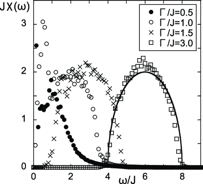
Figure 2: The correlation function $\chi(\omega)$ at $T=0$ for $N=10$. The solid line represents Eq.(26) with $\Gamma/J=3$.

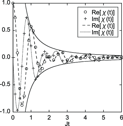
Figure 3: $\chi(t)$ at $T=0$ and $\Gamma/J=3$ obtained from the Fourier transformation of the data in Fig. 2. The points denote numerical data and the lines are analytical results. The solid lines are envelope curves $\pm\pi^{-1/2}(Jt)^{-3/2}$.

In order to check the analytical result at $T=0$ we carry out numerical calculation. The method of numerical analysis is based on the spectral decomposition of the correlation function $\chi(\omega)=\int dt\chi(t)\exp(i\omega t)$ as

$$\chi(\omega)=\left[\frac{\sum_{nm}e^{-\beta E_{n}}\delta\left(\omega-(E_{m}-E_{n})\right)\left|\langle n|\sigma^{z}_{i}|m\rangle\right|^{2}}{\sum_{n}e^{-\beta E_{n}}}\right],$$ (32)

where $n$ and $m$ denote energy eigenstates. This expression means that components in the summations contribute to $\chi(\omega)$ only when $\omega$ is equal to a difference of energies between two levels. At $T=0$, it is clear that only non-negative excitations are allowed and $\chi(\omega)$ forms a spectrum only in the range of positive $\omega$ as we showed above.

The quantity $\chi(\omega)$ is evaluated numerically by the diagonalization of the Hamiltonian. The number of sites is taken to be $N=10$, and the averaging is performed over more than 10000 samples. The zero-temperature results are shown in Fig. 2 and are compared with the analytical result (26). When the transverse field $\Gamma$ is not so small, we find a good agreement despite the fact that Eq.(26) is the Fourier transformation of the asymptotic form (24). We also note that a similar form of $\chi(\omega)$ has already been obtained in larger system sizes in Ref. AR, , which supports our analytical result as well.

We also show the correlation in real-time space in Fig. 3 by using numerical Fourier transformation of $\chi(\omega)$. The power index is estimated by linear fitting of $\ln|{\rm Re}\,\chi(t)|$ and $\ln|{\rm Im}\,\chi(t)|$ peaks versus $\ln t$. Due to the finite-size effect, the plot in Fig. 2 shows small oscillations and smooth tails, which leads to large deviations at large $t$ in Fig. 3. For this reason, the fitting is carried out within the region $t<5$. The power index is roughly estimated as 1.6, which is consistent with the analytical result, 1.5. We expect the small deviation from the analytical one also arises from the finite-size effect in small $t$ region, which is relatively smaller than in large $t$ region.

As in Fig. 2, when the transverse field $\Gamma$ is decreased the spectral band around $\omega=2\Gamma$ approaches the origin. We also observe a small sharp peak in the band around a certain value of $\omega$ with $\omega<2\Gamma$. This peak grows up and approaches the origin with increasing system size $N$. We expect this peak finally reaches the origin in infinite system size limit. Since the spin-glass order parameter $q$ is equal to the static part of $\chi(\tau)$ at $T=0$, KT $\chi(\omega=0)>0$ implies the spin-glass phase. Therefore we can interpret the emergence of the peak as a sign of the phase transition from the paramagnetic phase to the spin-glass phase. MH ; AR Although our system size $N=10$ is not large enough to find the transition point, the transition seems to happen at a value around $\Gamma\sim 1.5J$, which is consistent with the previous analyses. Since the main aim of the present paper is not to determine the precise value of the transition point, we defer the detailed analysis to a future work.

III Correlations at finite temperature

III.1 Numerical results

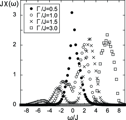
Figure 4: $\chi(\omega)$ at $T=2.0J$ for $N=10$.

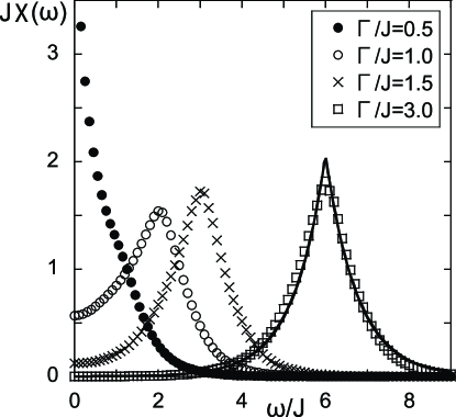
Figure 5: $\chi(\omega)$ at $T=\infty$ for $N=10$. The result is symmetric in $\omega$ as $\chi(-\omega)=\chi(\omega)$. The solid line is the result of the fitting using the function in Eq.(33) with $\bar{J}=0.76J$.

Next we move on to the finite temperature case. When the temperature is nonzero, the negative excitations are allowed and we expect double peaks around $\omega=\pm 2\Gamma$. These peaks finally become symmetric in the limit of $T\rightarrow\infty$, which can be understood from the spectral decomposition (32). The behavior at finite temperature is difficult to analyze since many energy levels contribute to the correlation function. In the imaginary-time path-integral formalism, the length of the integral path shrinks as the temperature is increased and the assumption of asymptotic decay in $\tau$ becomes invalid. For these reasons we do not apply imaginary-time path-integral formalism to finite temperature case.

We first observe the shape of $\chi(\omega)$ by the numerical method instead. The results at $T=2.0J$ and $T=\infty$ are shown in Figs. 4 and 5, respectively. As we expect, the double peaks are formed at finite temperature. When $\Gamma$ is not so small, the result at $T=\infty$ can be well fitted by the function

$$\chi(\omega)=\frac{\pi}{2\bar{J}}\left(e^{-|\omega-2\Gamma|/\bar{J}}+e^{-|\omega+2\Gamma|/\bar{J}}\right),$$ (33)

with a parameter $\bar{J}$. The result of fitting is also shown in Fig. 5. The parameter is taken as $\bar{J}=0.76J$, irrespective of the value of $\Gamma$. This form of fitting function is interpreted in the following.

III.2 Behavior at infinite temperature

Let us consider a perturbative analysis of the spectral representation at $T=\infty$

$$\chi(\omega)=\left[\frac{1}{2^{N}}\sum_{nm}\delta\left(\omega-(E_{m}-E_{n})\right)\left|\langle n|\sigma^{z}_{i}|m\rangle\right|^{2}\right].$$ (34)

In the limit of $J=0$, the eigenstates of the unperturbed Hamiltonian $\hat{H}_{0}=-\Gamma\sum_{i=1}^{N}\sigma_{i}^{x}$ are expressed by the eigenstates of $\sigma_{i}^{x}$. When the numbers of the spins pointing in the negative and the positive $x$ directions are $k$ and $N-k$, respectively, the unperturbed eigenenergy is given by $E^{(0)}_{k}=-(N-2k)\Gamma$ and the degree of degeneracy is ${}_{N}C_{k}=N!/k!(N-k)!$. The operator $\sigma_{i}^{z}$ flips the $i$th site spin and changes the number $k$ to $k\pm 1$, which determines the selection rule between the state $n$ and $m$ in Eq.(34). In the first order of perturbation theory, the Hamiltonian is diagonalized in a subspace characterized by the quantum number $k$. With this quantum number we obtain the approximate expression,

$$\chi(\omega) = \biggl{[}\frac{1}{2^{N}}\sum_{k=0}^{N-1}\sum_{\mu=1}^{{}_{N}C_{k}}\sum_{\nu=1}^{{}_{N}C_{k+1}}\left\{\delta\left(\omega-2\Gamma-(E_{k+1,\nu}^{(1)}-E_{k,\mu}^{(1)})\right)+\delta\left(\omega+2\Gamma+(E_{k+1,\nu}^{(1)}-E_{k,\mu}^{(1)})\right)\right\}$$ (35)

$$\times\left|\langle k+1,\nu|\sigma^{z}_{i}|k,\mu\rangle\right|^{2}\biggr{]},$$

where $\mu$ and $\nu$ denote the indices of degeneracy and the ranges depend on $k$. $E^{(1)}_{k,\mu}$ are eigenvalues at the first order and may be expressed by linear combinations of $J_{ij}$ as $E^{(1)}_{k,\mu}=\sum_{ij}m_{ij}^{(k,\mu)}J_{ij}$. Another form of $E^{(1)}_{k,\mu}$ as a function of $J_{ij}$ will not change the conclusion here. The averaging of Eq.(35) with respect to $J_{ij}$ yields a Gaussian factor as

$$\left[\delta\left(\omega-2\Gamma-\sum_{ij}m_{ij}J_{ij}\right)\right]\propto\exp\left\{-\frac{N(\omega-2\Gamma)^{2}}{2J^{2}\sum_{ij}m_{ij}^{2}}\right\}.$$ (36)

The contribution of Eq.(35) mainly comes from the sector with $k\sim N/2$, which is understood in conjunction with the factor $1/2^{N}$ in Eq.(35). For example, in the case of $k=0$ the number of the elements in the $\mu\nu$ sum is equal to $N$ and is negligible at $N\to\infty$ due to the multiplication by the factor $1/2^{N}$, whereas it is not suppressed when $k\sim N/2$.

Although it is hard to perform explicitly the perturbative calculation even at the first order, we easily see that the result is expressed by a linear combination of Gaussian functions as

$$\chi(\omega)=2\pi\int d\sigma P(\sigma)\left[\exp\left\{-\frac{(\omega-2\Gamma)^{2}}{2\sigma^{2}}\right\}+\exp\left\{-\frac{(\omega+2\Gamma)^{2}}{2\sigma^{2}}\right\}\right],$$ (37)

where $P(\sigma)$ is the distribution function of the variance $\sigma$. From this expression, we find that result (33) can be reproduced by assuming the Gaussian distribution $P(\sigma)\propto\exp(-\sigma^{2}/2\bar{J}^{2})$. The Fourier transformation of Eq.(33) gives

$$\chi(t)=\frac{\cos(2\Gamma t)}{1+\bar{J}^{2}t^{2}}.$$ (38)

This shows that the correlation asymptotically decays as $t^{-2}$. We must note that this index is obtained by a different mechanism as Ref. MH, where the same value of the index is concluded at zero temperature.

III.3 Classical and quantum paramagnetic phase

At finite temperature, the spin-glass phase is suppressed in increasing $T$ and disappears at $T=J$. MPV ; Nishimori The second-order phase-transition curve, namely, the spin-glass phase boundary, runs from $T=0$, $\Gamma\sim 1.5J$ to $T=J$, $\Gamma=0$ on $T$-$\Gamma$ plane. On the other hand, in Sec. II we saw the change in the behavior of $\chi(t)$ at zero temperature when $\Gamma$ is varied, and this change is expected to be persistent up to higher-temperature region than the spin-glass phase boundary. We can attribute this change to the one in moving across the boundary between the quantum paramagnetic (QP) and the classical paramagnetic (CP) phases, rather than between the spin-glass phase and one of the paramagnetic phases.

The existence of the phase transition between the CP and the QP phases has already been found in the $p$-body interaction spin-glass model in a transverse field defined by the Hamiltonian

$$\hat{H}=-\sum_{i_{1}<i_{2}<\cdots<i_{p}}J_{i_{1}i_{2}\cdots i_{p}}\sigma^{z}_{i_{1}}\sigma^{z}_{i_{2}}\cdots\sigma^{z}_{i_{p}}-\Gamma\sum_{i}\sigma^{x}_{i}.$$ (39)

The interaction $J_{i_{1}i_{2}\cdots i_{p}}$ is random and the average is taken with Gaussian probability distribution. At $p\to\infty$ this model is known as the random energy model and exhibits first-order phase transition between the CP and the QP phases. REM The imaginary-time-correlation function at the QP phase can be calculated from the self-consistent equation in terms of $\chi(\tau)$,

$$\chi(\tau)=\left<s^{(1)}_{z}(\tau)s^{(1)}_{z}(0)\exp\left\{\frac{pJ^{2}}{4}\sum_{\alpha=1}^{n}\int_{0}^{\beta}d\tau_{1}\int_{0}^{\beta}d\tau_{2}\,s_{z}^{(\alpha)}(\tau_{1})\chi^{p-1}(\tau_{1}-\tau_{2})s_{z}^{(\alpha)}(\tau_{2})\right\}\right>_{\Gamma}.$$ (40)

The factor $\chi^{p-1}$ goes to zero at $p\to\infty$ unless $\chi=1$. From this, it is clear the zeroth-order calculation becomes exact,

$$\chi(\tau)=D_{\Gamma}(\tau)=\frac{e^{\beta\Gamma-2\Gamma\tau}+e^{-\beta\Gamma+2\Gamma\tau}}{e^{\beta\Gamma}+e^{-\beta\Gamma}}.$$ (41)

The phase-transition point cannot be determined from this equation for the QP phase but can be determined by the static part of the correlation function for the CP phase. Considering the condition of the vanishing static part, we obtain a discontinuous change from $\chi(\tau)=1$ to Eq.(41), which also tells us the boundary between the CP and the QP phases reaches $T=\infty$. When $p$ takes a large but finite value, the phase-transition line is terminated at a certain finite temperature value and the transition between the CP and the QP phases turns to crossover. p

Our numerical analysis for the SK ($p=2$) model shows that the semicircle form changes to a broader one at finite temperature. The long tail of the spectrum reaches the origin $\omega=0$, just as Eq.(33). We also observe that a sharp peak around the origin, which was considered a precursor of the spin-glass transition for finite systems, is suppressed at finite temperature. These observations imply that the spectrum change at finite temperature indicates a crossover between the CP and the QP phases. This picture is supported by the analysis in Ref. KT, where a smooth change in the static part of the correlation function was obtained at $T>0$. However, it is known in a Langevin dynamics model of $p$-body interaction spin glass p2 that the behavior at $p>2$ should be distinguished from the one with $p=2$. Our numerical calculation is carried out for rather small systems, and it is fair to say that our analysis is not conclusive and further studies are required to determine the properties of the finite temperature phase diagram.

IV Conclusions

In conclusion, we have calculated the dynamical correlation function (1) in the transverse SK model (2). Our main results are Eqs.(24) and (26) at $T=0$, and Eqs.(33) and (38) at $T=\infty$. For large transverse field, the correlation function asymptotically decays in time $t$ as $t^{-3/2}$ at $T=0$ and $t^{-2}$ at $T=\infty$. The results of our analysis are different from those of previous works at $T=0$. MH ; YSR ; RG ; GR In the present spin system, it is the crucial point in the analysis that the simple Wick theorem cannot be applied to the multicorrelations of the spin operators. It was shown in Ref. WSC, that the factorization for Gaussian variables is modified in the case of spin operators and a sign factor is introduced to respect time ordering of operators. We showed that the correct procedure leads to a different form of real-time correlation from the known one.

In the present paper, we have analyzed the infinite range model to focus on the time dependence of the correlation function. It is important to study how the present result is changed at finite-dimensional models with finite range interactions. Spatial correlation can be related to time correlation; therefore the result of such study will be useful. With regard to critical exponent, there is an argument that the dynamic critical exponent $z$ is related to the power index of the time-correlation function discussed in the present paper. ARi In addition, in low-dimensional systems it is inferred from the general considerations Sachdev that correlation function is significantly affected by Griffiths-McCoy singularities. GM

Application to other random quantum systems is also an interesting future work. For the random quantum Heisenberg model, the correlation function in Fourier-transformed space, $\chi(\omega)$, was numerically analyzed in Refs. AR, and AR2, . It is interesting to analyze the correlation in real-time space by using the analytical method developed here, and this will be our future work.

References

- (1) M. Mézard, G. Parisi, and M.A. Virasoro, Spin Glass Theory and Beyond (World Scientific, Singapore, 1987).
- (2) H. Nishimori, Statistical Physics of Spin Glasses and Information Processing: An Introduction (Oxford University Press, Oxford, 2001).
- (3) D. Sherrington and S. Kirkpatrick, Phys. Rev. Lett. 35, 1792 (1975).
- (4) A.J. Bray and M.A. Moore, J. Phys. C 13, L655 (1980).
- (5) B.S. Chakrabarti, A. Dutta, and P. Sen, Quantum Ising Phases and Transitions in Transverse Ising Models (Springer, Berlin, 1996).
- (6) S. Sachdev, Quantum Phase Transitions (Cambridge University Press, Cambridge, 1999).
- (7) K. Takahashi, Phys. Rev. B 76, 184422 (2007).
- (8) A. Georges, G. Kotliar, W. Krauth, and M.J. Rozenberg, Rev. Mod. Phys. 68, 13 (1996).
- (9) J. Miller and D.A. Huse, Phys. Rev. Lett. 70, 3147 (1993).
- (10) J. Ye, S. Sachdev, and N. Read, Phys. Rev. Lett. 70, 4011 (1993).
- (11) M.J. Rozenberg and D.R. Grempel, Phys. Rev. Lett. 81, 2550 (1998).
- (12) D.R. Grempel and M.J. Rozenberg, Phys. Rev. B 60, 4702 (1999).
- (13) J.V. Alvarez and F. Ritort, J. Phys. A 29, 7355 (1996).
- (14) L. Arrachea and M.J. Rozenberg, Phys. Rev. Lett. 86, 5172 (2001).
- (15) P.W. Anderson and G. Yuval, Phys. Rev. Lett. 23, 89 (1969); G. Yuval and P.W. Anderson, Phys. Rev. B 1, 1522 (1970); P.W. Anderson, G. Yuval, and D.R. Hamann, ibid. 1, 4464 (1970).
- (16) Y.Y. Goldschmidt, Phys. Rev. B 41, 4858 (1990); T. Obuchi, H. Nishimori, and D. Sherrington, J. Phys. Soc. Jpn. 76, 054002 (2007).
- (17) L. De Cesare, K. Lukierska-Walasek, I. Rabuffo, and K. Walasek, J. Phys. A 29, 1605 (1996); T.M. Nieuwenhuizen and F. Ritort, Physica A 250, 8 (1998).
- (18) T.R. Kirkpatrick and D. Thirumalai, Phys. Rev. Lett. 58, 2091 (1987); Phys. Rev. B 36, 5388 (1987); A. Crisanti, H. Horner, and H.-J. Sommers, Z. Phys. B: Condens. Matter 92, 257 (1993).
- (19) Y.L. Wang, S. Shtrikman, and H. Callen, Phys. Rev. 148, 419 (1966).
- (20) R.B. Griffiths, Phys. Rev. Lett. 23, 17 (1969); B.M. McCoy, ibid. 23, 383 (1969).
- (21) L. Arrachea and M.J. Rozenberg, Phys. Rev. B 65, 224430 (2002).