Convergence of the critical finite-range contact process
to super-Brownian motion above the upper critical dimension:
I. The higher-point functions

Abstract

We consider the critical spread-out contact process in ${{{\mathbb{Z}}}^{d}}$ with $d\geq 1$, whose infection range is denoted by $L\geq 1$. In this paper, we investigate the higher-point functions $\tau_{\vec{t}}^{\scriptscriptstyle(r)}(\vec{x})$ for $r\geq 3$, where $\tau_{\vec{t}}^{\scriptscriptstyle(r)}(\vec{x})$ is the probability that, for all $i=1,\dots,r-1$, the individual located at $x_{i}\in{{{\mathbb{Z}}}^{d}}$ is infected at time $t_{i}$ by the individual at the origin $o\in{{{\mathbb{Z}}}^{d}}$ at time 0. Together with the results of the 2-point function in [15], on which our proofs crucially rely, we prove that the $r$-point functions converge to the moment measures of the canonical measure of super-Brownian motion above the upper critical dimension 4. We also prove partial results for $d\leq 4$ in a local mean-field setting.

The proof is based on the lace expansion for the time-discretized contact process, which is a version of oriented percolation in ${{{\mathbb{Z}}}^{d}}\times\varepsilon{\mathbb{Z}}_{+}$, where $\varepsilon\in(0,1]$ is the time unit. For ordinary oriented percolation (i.e., $\varepsilon=1$), we thus reprove the results of [19]. The lace expansion coefficients are shown to obey bounds uniformly in $\varepsilon\in(0,1]$, which allows us to establish the scaling results also for the contact process (i.e., $\varepsilon\downarrow 0$). We also show that the main term of the vertex factor $V$, which is one of the non-universal constants in the scaling limit, depends explicitly on the time unit as $2-\varepsilon$, while the main terms of the other non-universal constants are independent of $\varepsilon$.

The lace expansion we develop in this paper is adapted to both the $r$-point function and the survival probability. This unified approach makes it easier to relate the expansion coefficients derived in this paper and the expansion coefficients for the survival probability, which will be reported in Part II [17].

1 Introduction and results

1.1 Introduction

The contact process is a model for the spread of an infection among individuals in the $d$-dimensional integer lattice ${\mathbb{Z}}^{d}$. Suppose that the origin $o\in{{{\mathbb{Z}}}^{d}}$ is the only infected individual at time 0, and assume for now that every infected individual may infect a healthy individual at a distance less than $L\geq 1$. We refer to this type of model as the spread-out contact process. The rate of infection is denoted by $\lambda$, and it is well known that there is a phase transition in $\lambda$ at a critical value $\lambda_{\rm c}\in(0,\infty)$ (see, e.g., [21]).

In the previous paper [15], and following the idea of [22], we proved the 2-point function results for the contact process for $d>4$ via a time discretization, as well as a partial extension to $d\leq 4$. The discretized contact process is a version of oriented percolation in ${{{\mathbb{Z}}}^{d}}\times\varepsilon{\mathbb{Z}}_{+}$, where $\varepsilon\in(0,1]$ is the time unit. The proof is based on the strategy for ordinary oriented percolation ($\varepsilon=1$), i.e., on the application of the lace expansion and an adaptation of the inductive method so as to deal with the time discretization.

In this paper, we use the 2-point function results in [15] as a key ingredient to show that, for any $r\geq 3$, the $r$-point functions of the critical contact process for $d>4$ converge to those of the canonical measure of super-Brownian motion, as was proved in [19] for ordinary oriented percolation. We follow the strategy in [19] to analyze the lace expansion, but derive an expansion which is different from the expansion used in [19]. The lace expansion used in this paper is closely related to the expansion in [14] for the oriented-percolation survival probability. The latter was used in [13] to show that the probability that the oriented-percolation cluster survives up to time $n$ decays proportionally to $1/n$. Due to this close relation, we can reprove an identity relating the constants arising in the scaling limit of the 3-point function and the survival probability, as was stated in [12, Theorem 1.5] for oriented percolation.

The main selling points of this paper in comparison to other papers on the topic are the following:

1. Our proof yields a simplification of the expansion argument, which is still inherently difficult, but has been simplified as much as possible, making use of and extending the combined insights of [9, 14, 15, 19].

2. The expansion for the higher-point functions yields similar expansion coefficients to those for the survival probability in [14], thus making the investigation of the contact-process survival probability more efficient and allowing for a direct comparison of the various constants arising in the 2- and 3-point functions and the survival probability. This was proved for oriented percolation in [12, Theorem 1.5], which, on the basis of the expansion in [18], was not directly possible.

3. The extension of the results to certain local mean-field limit type results in low dimensions, as was initiated in [5] and taken up again in [15].

4. A simplified argument for the continuum limit of the discretized model, which was performed in [15] through an intricate weak convergence argument, and which in the current paper is replaced by a soft argument on the basis of subsequential limits and uniformity of our bounds.

The investigation of the contact-process survival probability is deferred to Part II of this paper [17], in which we also discuss the implications of our results for the convergence of the critical spread-out contact process towards super-Brownian motion, in the sense of convergence of finite-dimensional distributions [20]. See also [11] and [24] for more expository discussions of the various results for oriented percolation and the contact process for $d>4$, and [25] for a detailed discussion of the applications of the lace expansion.

1.2 Main results

We define the spread-out contact process as follows. Let ${\bf C}_{t}\subseteq{\mathbb{Z}}^{d}$ be the set of infected individuals at time $t\in{\mathbb{R}}_{+}$, and let ${\bf C}_{0}=\{o\}.$ An infected site $x$ recovers in a small time interval $[t,t+\varepsilon]$ with probability $\varepsilon+o(\varepsilon)$ independently of $t$, where $o(\varepsilon)$ is a function that satisfies $\lim_{\varepsilon\downarrow 0}o(\varepsilon)/\varepsilon=0$. In other words, $x\in{\bf C}_{t}$ recovers at rate 1. A healthy site $x$ gets infected, depending on the status of its neighboring sites, at rate $\lambda\sum_{y\in{\bf C}_{t}}D(x-y)$, where $\lambda\geq 0$ is the infection rate. We denote the associated probability measure by ${\mathbb{P}}^{\lambda}$. We assume that the function $D:{{{\mathbb{Z}}}^{d}}\to[0,1]$ is a probability distribution which is symmetric with respect to the lattice symmetries. Further assumptions on $D$ involve a parameter $L\geq 1$ which serves to spread out the infections, and will be taken to be large. In particular, we require that $D(o)=0$ and $\|D\|_{\infty}\equiv\sup_{x\in{{{\mathbb{Z}}}^{d}}}D(x)\leq CL^{-d}$. Moreover, with $\sigma$ defined as

$$\sigma^{2}=\sum_{x}|x|^{2}D(x),$$ (1.1)

where $|\cdot|$ denotes the Euclidean norm on ${\mathbb{R}}^{d}$, we require that $C_{1}L\leq\sigma\leq C_{2}L$ and that there exists a $\Delta>0$ such that

$$\sum_{x}|x|^{2+2\Delta}D(x)\leq CL^{2+2\Delta}.$$ (1.2)

See [15, Section 5] for the precise assumptions on $D$. A simple example of $D$ is

$$D(x)=\frac{\mathbbm{1}{\scriptstyle\{0<\|x\|_{\infty}\leq L\}}}{(2L+1)^{d}-1},$$ (1.3)

which is the uniform distribution on the cube of radius $L$.

For $r\geq 2$, $\vec{t}=(t_{1},\dots,t_{r-1})\in{\mathbb{R}}_{+}^{r-1}$ and $\vec{x}=(x_{1},\dots,x_{r-1})\in{\mathbb{Z}}^{(r-1)d}$, we define the $r$-point function as

$$\tau_{\vec{t}}^{\lambda}(\vec{x})={\mathbb{P}}^{\lambda}(x_{i}\in{\bf C}_{t_{i}}~{}\forall i=1,\dots,r-1).$$ (1.4)

For a summable function $f\colon{\mathbb{Z}}^{d}\to{\mathbb{R}}$, we define its Fourier transform for $k\in[-\pi,\pi]^{d}$ by

$$\hat{f}(k)=\sum_{x\in{\mathbb{Z}}^{d}}e^{ik\cdot x}f(x).$$ (1.5)

By the results in [8] and the extension in [2] to the spread-out model, there exists a unique critical point $\lambda_{\rm c}\in(0,\infty)$ such that

$$\int_{0}^{\infty}dt\;\hat{\tau}_{t}^{\lambda}(0)\begin{cases}<\infty,&\mbox{if }\lambda<\lambda_{\rm c},\\ =\infty,&\mbox{otherwise},\end{cases} \lim_{t\uparrow\infty}{\mathbb{P}}^{\lambda}({\bf C}_{t}\neq\varnothing)\begin{cases}=0,&\mbox{if }\lambda\leq\lambda_{\rm c},\\ >0,&\mbox{otherwise}.\end{cases}$$ (1.6)

We will next investigate the sufficiently spread-out contact process at the critical value $\lambda_{\rm c}$ for $d>4$, as well as a local mean-field limit when $d\leq 4$.

1.3 Previous results for the 2-point function

We first state the results for the 2-point function proved in [15]. Those results will be crucial for the current paper. In the statements, $\sigma$ is defined in (1.1) and $\Delta$ in (1.2).

Besides the high-dimensional setting for $d>4$, we also consider a low-dimensional setting, i.e., $d\leq 4$. In this case, the contact process is not believed to be in the mean-field regime, and Gaussian asymptotics are thus not expected to hold as long as $L$ remains finite. However, following the rescaling of Durrett and Perkins in [5], we have proved Gaussian asymptotics when range and time grow simultaneously [15]. We suppose that the infection range grows as

$$L_{{\scriptscriptstyle T}}=L_{1}\,T^{b},$$ (1.7)

where $L_{1}\geq 1$ is the initial infection range and $T\geq 1$. We denote by $\sigma_{{\scriptscriptstyle T}}^{2}$ the variance of ${D=D_{{\scriptscriptstyle T}}}$ in this situation. We will assume that

$$\alpha=bd+\frac{d-4}{2}>0.$$ (1.8)

Theorem 1.1 (Gaussian asymptotics two-point function).

1. Let $d>4$, $\delta\in(0,1\wedge\Delta\wedge\frac{d-4}{2})$ and $L\gg 1$. There exist positive and finite constants $v,A$ (depending on $d$ and $L$) and $C_{1},C_{2}$ (depending only on $d$) such that

   $$\hat{\tau}_{t}^{\lambda_{\rm c}}\big{(}\tfrac{k}{\sqrt{v\sigma^{2}t}}\big{)}=A\,e^{-\frac{|k|^{2}}{2d}}\Big{(}1+O\big{(}|k|^{2}(1+t)^{-\delta}\big{)}+O\big{(}(1+t)^{-(d-4)/2}\big{)}\Big{)},$$ (1.9)

   $$\frac{1}{\hat{\tau}_{t}^{\lambda_{\rm c}}(0)}\sum_{x}|x|^{2}\tau_{t}^{\lambda_{\rm c}}(x)=v\sigma^{2}t\Big{(}1+O\big{(}(1+t)^{-\delta}\big{)}\Big{)},$$ (1.10)

   $$C_{1}L^{-d}(1+t)^{-d/2}\leq\|\tau_{t}^{\lambda_{\rm c}}\|_{\scriptscriptstyle\infty}\leq e^{-t}+C_{2}L^{-d}(1+t)^{-d/2},$$ (1.11)

   with the error estimate in (1.9) uniform in $k\in{\mathbb{R}}^{d}$ with ${|k|^{2}/\log(2+t)}$ sufficiently small. Moreover,

   $$\lambda_{\rm c}=1+O(L^{-d}), A=1+O(L^{-d}), v=1+O(L^{-d}).$$ (1.12)

2. Let $d\leq 4$, $\delta\in(0,1\wedge\Delta\wedge\alpha)$ and $L_{1}\gg 1$. There exist $\lambda_{{\scriptscriptstyle T}}=1+O(T^{-\mu})$ for some $\mu\in(0,\alpha-\delta)$ and $C_{1},C_{2}\in(0,\infty)$ (depending only on $d$) such that, for every $0<t\leq\log T$,

   $$\hat{\tau}_{Tt}^{\lambda_{T}}\big{(}\tfrac{k}{\sqrt{\sigma_{{\scriptscriptstyle T}}^{2}Tt}}\big{)}=e^{-\frac{|k|^{2}}{2d}}\Big{(}1+O(T^{-\mu})+O\big{(}|k|^{2}(1+Tt)^{-\delta}\big{)}\Big{)},$$ (1.13)

   $$\frac{1}{\hat{\tau}_{Tt}^{\lambda_{{\scriptscriptstyle T}}}(0)}\sum_{x}|x|^{2}\tau_{Tt}^{\lambda_{{\scriptscriptstyle T}}}(x)=\sigma_{{\scriptscriptstyle T}}^{2}Tt\Big{(}1+O(T^{-\mu})+O\big{(}(1+Tt)^{-\delta}\big{)}\Big{)},$$ (1.14)

   $$C_{1}L_{{\scriptscriptstyle T}}^{-d}(1+Tt)^{-d/2}\leq\|\tau_{Tt}^{\lambda_{T}}\|_{\scriptscriptstyle\infty}\leq e^{-Tt}+C_{2}L_{{\scriptscriptstyle T}}^{-d}(1+Tt)^{-d/2},$$ (1.15)

   with the error estimate in (1.13) uniform in $k\in{\mathbb{R}}^{d}$ with ${|k|^{2}/\log(2+Tt)}$ sufficiently small.

In the rest of the paper, we will always work at the critical value, i.e., we take $\lambda=\lambda_{\rm c}$ for $d>4$ and $\lambda=\lambda_{\scriptscriptstyle T}$ as in Theorem 1.1(ii) for $d\leq 4$. We will often omit the $\lambda$-dependence and write $\tau_{\vec{t}}^{{\scriptscriptstyle{({r}})}}(\vec{x})=\tau_{\vec{t}}^{\lambda}(\vec{x})$ to emphasize the number of arguments of $\tau_{\vec{t}}^{\lambda}(\vec{x})$.

While $\tau_{t}^{\lambda_{\rm c}}(x)$ tells us what paths in a critical cluster look like, the critical $r$-point functions give us information about the branching structure of critical clusters. Our goal in this paper is to prove that the suitably scaled critical $r$-point functions converge to those of the canonical measure of super-Brownian motion (SBM).

1.4 The $r$-point function for $r\geq 3$

To state the result for the $r$-point function for $r\geq 3$, we begin by describing the Fourier transforms of the moment measures of SBM. These are most easily defined recursively, and will serve as the limits of the $r$-point functions. We define

$$\hat{M}_{t}^{{\scriptscriptstyle{({1}})}}(k)=e^{-\frac{|k|^{2}}{2d}t},\qquad k\in{\mathbb{R}}^{d},\,t\in{\mathbb{R}}_{+},$$ (1.16)

and define recursively, for $l\geq 2$,

$$\hat{M}_{\vec{t}}^{{\scriptscriptstyle{({l}})}}(\vec{k})=\int_{0}^{\underline{t}}dt\,\hat{M}_{t}^{{\scriptscriptstyle{({1}})}}(k_{1}+\cdots+k_{l})\sum_{I\subset J_{1}:|I|\geq 1}\hat{M}_{\vec{t}_{I}-t}^{{\scriptscriptstyle{({|I|}})}}(\vec{k}_{I})\,\hat{M}_{\vec{t}_{J\setminus I}-t}^{{\scriptscriptstyle{({l-|I|}})}}(\vec{k}_{J\setminus I}),\qquad\vec{k}\in{\mathbb{R}}^{dl},\,\vec{t}\in{\mathbb{R}}_{+}^{l},$$ (1.17)

where $J=\{1,\dots,l\}$, $J_{1}=J\setminus\{1\}$, $\underline{t}=\min_{i}t_{i}$, $\vec{t}_{I}$ is the vector consisting of $t_{i}$ with $i\in I$, and $\vec{t}_{I}-t$ is subtraction of $t$ from each component of $\vec{t}_{I}$. The quantity $\hat{M}_{\vec{t}}^{{\scriptscriptstyle{({l}})}}(\vec{k})$ is the Fourier transform of the $l^{\rm th}$ moment measure of the canonical measure of SBM (see [19, Sections 1.2.3 and 2.3] for more details on the moment measures of SBM).

The following is the result for the $r$-point function for $r\geq 3$ linking the critical contact process and the canonical measure of SBM:

Theorem 1.2 (Convergence of $r$-point functions to SBM moment measures).

1. Let $d>4$, $\lambda=\lambda_{\rm c}$, $\vec{k}\in{\mathbb{R}}^{d(r-1)}$, $\vec{t}\in(0,\infty)^{r-1}$ and $\delta,L,v,A$ be the same as in Theorem 1.1(i). There exists $V=V(d,L)$ such that, for every $r\geq 2$ and as $T\uparrow\infty$,

   $$\hat{\tau}_{T\vec{t}}^{\scriptscriptstyle(r)}\big{(}\tfrac{\vec{k}}{\sqrt{v\sigma^{2}T}}\big{)}=A\,(A^{2}VT)^{r-2}\Big{(}\hat{M}_{\vec{t}}^{\scriptscriptstyle(r-1)}(\vec{k})+O(T^{-\delta})\Big{)},$$ (1.18)

   uniformly in $\vec{k}\in{\mathbb{R}}^{d(r-1)}$ with $\sum_{i=1}^{r-1}|k_{i}|^{2}$ bounded. Moreover, $V=2+O(L^{-d})$.

2. Let $d\leq 4$, $\vec{k}\in{\mathbb{R}}^{d(r-1)}$, $\vec{t}\in(0,\infty)^{r-1}$ and let $\delta,L_{1},\lambda_{{\scriptscriptstyle T}},\mu$ be the same as in Theorem 1.1(ii). For every $r\geq 2$, $0<\max_{i}s_{i}\leq\log T$ and as $T\uparrow\infty$,

   $$\hat{\tau}_{T\vec{t}}^{{\scriptscriptstyle{({r}})}}\big{(}\tfrac{\vec{k}}{\sqrt{\sigma_{{\scriptscriptstyle T}}^{2}T}}\big{)}=(2T)^{r-2}\Big{(}\hat{M}_{\vec{t}}^{{\scriptscriptstyle{({r-1}})}}(\vec{k})+O(T^{-\mu\wedge\delta})\Big{)},$$ (1.19)

   uniformly in $\vec{k}\in{\mathbb{R}}^{d(r-1)}$ with $\sum_{i=1}^{r-1}|k_{i}|^{2}$ bounded.

Since the statements for $r=2$ in Theorem 1.2 follow from Theorem 1.1, we only need prove Theorem 1.2 for $r\geq 3$. As described in more detail in Part II [17], Theorems 1.1–1.2 can be rephrased to say that, under their hypotheses, the moment measures of the rescaled critical contact process converge to those of the canonical measure of SBM. The consequences of this result for the convergence of the critical contact process towards SBM will be deferred to [17].

Theorem 1.2 will be proved using the lace expansion, which perturbs the $r$-point functions for the critical contact process around those for critical branching random walk. To derive the lace expansion, we use a time-discretization. The time-discretized contact process has a parameter $\varepsilon\in(0,1]$. The boundary case $\varepsilon=1$ corresponds to ordinary oriented percolation, while the limit $\varepsilon\downarrow 0$ yields the contact process. We will prove Theorem 1.2 for the time-discretized contact process and prove that the error terms are uniform in the discretization parameter $\varepsilon$. As a consequence, we will reprove Theorem 1.2 for oriented percolation. The first proof of Theorem 1.2 for oriented percolation appeared in [19].

In [3, 4], spread-out oriented percolation is investigated in the setting where the finite variance condition (1.2) fails, and it was shown that for certain infinite variance step distributions $D$ in the domain of attraction of an $\alpha$-stable distribution, the Fourier transform of two-point function converges to the one of an $\alpha$-stable random variable, when $d>2\alpha$ and $\alpha\in(0,2)$. We conjecture that, in this case, the limits of the $r$-point functions satisfy a limiting result similarly to (1.18) when the argument in the $r$-point function in (1.18) is replaced by $\tfrac{\vec{k}}{vT^{1/\alpha}}$ for some $v>0$, and where the limit corresponds to the moment measures of a super-process where the motion is $\alpha$-stable and the branching has finite variance (in the terminology of [6, Definition 1.33, p. 22], this corresponds to the $(\alpha,d,1)$-superprocess and SBM corresponds to $\alpha=2$). These limiting moment measures should satisfy (1.17), but (1.16) is replaced by $e^{-|k|^{\alpha}t}$, which is the Fourier transform of an $\alpha$-stable motion at time $t$.

1.5 Organization

The paper is organised as follows. In Section 2, we will describe the time-discretization, state the results for the time-discretized contact process and give an outline of the proof. In this outline, the proof of Theorem 1.2 will be reduced to Propositions 2.2 and 2.4. In Proposition 2.2, we state the bounds on the expansion coefficients arising in the expansion for the $r$-point function. In Proposition 2.4, we state and prove that the sum of these coefficients converges, when appropriately scaled and as $\varepsilon\downarrow 0$. The rest of the paper is devoted to the proof of Propositions 2.2 and 2.4. In Sections 3–4, we derive the lace expansion for the $r$-point function, thus identifying the lace-expansion coefficients. In Sections 5–7, we prove the bounds on the coefficients and thus prove Proposition 2.2.

2 Outline of the proof

In this section, we give an outline of the proof of Theorem 1.2, and reduce this proof to Propositions 2.2 and 2.4. This section is organized as follows. In Section 2.1, we describe the time-discretized contact process. In Section 2.2, we outline the lace expansion for the $r$-point functions and state the bounds on the coefficients in Proposition 2.2. In Section 2.4, we prove Theorem 1.2 for the time-discretized contact process subject to Propositions 2.2. Finally, in Section 2.5, we prove Proposition 2.4, and complete the proof of Theorem 1.2 for the contact process.

2.1 Discretization

In this section, we introduce the discretized contact process, which is an interpolation between oriented percolation on the one hand, and the contact process on the other. This section contains the same material as [15, Section 2.1]. We shall also use the notation ${\mathbb{N}}=\{1,2,\ldots\}$, ${\mathbb{Z}}_{+}=\{0\}~{}\dot{\cup}~{}{\mathbb{N}}$ and ${\mathbb{R}}_{+}=[0,\infty)$.

The contact process can be constructed using a graphical representation as follows. We consider ${{{\mathbb{Z}}}^{d}}\times{\mathbb{R}}_{+}$ as space-time. Along each time line $\{x\}\times{\mathbb{R}}_{+}$, we place points according to a Poisson process with intensity 1, independently of the other time lines. For each ordered pair of distinct time lines from $\{x\}\times{\mathbb{R}}_{+}$ to $\{y\}\times{\mathbb{R}}_{+}$, we place directed bonds $((x,\,t),(y,\,t))$, $t\geq 0$, according to a Poisson process with intensity $\lambda\,D(y-x)$, independently of the other Poisson processes. A site $(x,s)$ is said to be connected to $(y,t)$ if either $(x,s)=(y,t)$ or there is a non-zero path in ${{{\mathbb{Z}}}^{d}}\times{\mathbb{R}}_{+}$ from $(x,s)$ to $(y,t)$ using the Poisson bonds and time line segments traversed in the increasing time direction without traversing the Poisson points. The law of $\{{\bf C}_{t}\}_{t\in{\mathbb{R}}_{+}}$ defined in Section 1.2 is equal to that of $\big{\{}\{x\in{{{\mathbb{Z}}}^{d}}:(o,\,0)$ is connected to $(x,\,t)\}\big{\}}_{t\in{\mathbb{R}}_{+}}$.

We follow [22] and consider an oriented percolation process in ${{{\mathbb{Z}}}^{d}}\times\varepsilon{\mathbb{Z}}_{+}$ with $\varepsilon\in(0,1]$ being a discretization parameter as follows. A directed pair $b=((x,t),(y,t+\varepsilon))$ of sites in ${{{\mathbb{Z}}}^{d}}\times\varepsilon{\mathbb{Z}}_{+}$ is called a bond. In particular, $b$ is said to be temporal if $x=y$, otherwise spatial. Each bond is either occupied or vacant independently of the other bonds, and a bond $b=((x,t),(y,t+\varepsilon))$ is occupied with probability

$$p_{\varepsilon}(y-x)=\begin{cases}1-\varepsilon,&\mbox{if }x=y,\\ \lambda\varepsilon\,D(y-x),&\mbox{otherwise},\end{cases}$$ (2.1)

provided that $\sup_{x}p_{\varepsilon}(x)\leq 1$. We denote the associated probability measure by ${\mathbb{P}}_{\varepsilon}^{\lambda}$. It has been proved in [2] that ${\mathbb{P}}_{\varepsilon}^{\lambda}$ weakly converges to ${\mathbb{P}}^{\lambda}$ as $\varepsilon\downarrow 0$. See Figure 1 for a graphical representation of the contact process and the discretized contact process. As explained in more detail in Section 2.2, we prove our main results by proving the results first for the discretized contact process, and then taking the continuum limit $\varepsilon\downarrow 0$.

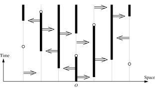
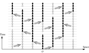
Figure 1: Graphical representation of the contact process and the discretized contact process.

We denote by $(x,s)\longrightarrow(y,t)$ the event that $(x,s)$ is connected to $(y,t)$, i.e., either $(x,s)=(y,t)$ or there is a non-zero path in ${{{\mathbb{Z}}}^{d}}\times\varepsilon{\mathbb{Z}}_{+}$ from $(x,s)$ to $(y,t)$ consisting of occupied bonds. The $r$-point functions, for $r\geq 2$, $\vec{t}=(t_{1},\ldots,t_{r-1})\in\varepsilon{\mathbb{Z}}_{+}^{r-1}$ and $\vec{x}=(x_{1},\ldots,x_{r-1})\in{\mathbb{Z}}^{d(r-1)}$, are defined as

$$\tau_{\vec{t};\varepsilon}^{\scriptscriptstyle(r)}(\vec{x})={\mathbb{P}}_{\varepsilon}^{\lambda}\big{(}(o,0)\longrightarrow(x_{i},t_{i})~{}~{}\forall i=1,\ldots,r-1\big{)}.$$ (2.2)

Similarly to (1.6), the discretized contact process has a critical value $\lambda_{\rm c}^{{\scriptscriptstyle{({\varepsilon}})}}$ satisfying

$$\varepsilon\sum_{t\in\varepsilon{\mathbb{Z}}_{+}}\hat{\tau}_{t;\varepsilon}^{\lambda}(0)\begin{cases}<\infty,&\mbox{if }\lambda<\lambda_{\rm c}^{\scriptscriptstyle(\varepsilon)},\\ =\infty,&\mbox{otherwise},\end{cases} \lim_{t\uparrow\infty}{\mathbb{P}}_{\varepsilon}^{\lambda}({\bf C}_{t}\neq\varnothing)\begin{cases}=0,&\mbox{if }\lambda\leq\lambda_{\rm c}^{\scriptscriptstyle(\varepsilon)},\\ >0,&\mbox{otherwise}.\end{cases}$$ (2.3)

The discretization procedure will be essential in order to derive the lace expansion for the $r$-point functions for $r\geq 3$, as it was for the 2-point function in [15].

Note that for $\varepsilon=1$ the discretized contact process is simply oriented percolation. Our main result for the discretized contact process is the following theorem, similar to Theorem 1.2:

Theorem 2.1 (Convergence of time-discretized $r$-point functions to SBM moment measures).

1. Let $d>4$, $\lambda=\lambda_{\rm c}^{\scriptscriptstyle(\varepsilon)}$, $\vec{k}\in{\mathbb{R}}^{d(r-1)}$, $\vec{t}\in(0,\infty)^{r-1}$, $\delta\in(0,1\wedge\Delta\wedge\frac{d-4}{2})$ and $L\gg 1$, as in Theorem 1.1(i). There exist $A^{\scriptscriptstyle(\varepsilon)}=A^{\scriptscriptstyle(\varepsilon)}(d,L)$, $v^{\scriptscriptstyle(\varepsilon)}=v^{\scriptscriptstyle(\varepsilon)}(d,L)$, $V^{\scriptscriptstyle(\varepsilon)}=V^{\scriptscriptstyle(\varepsilon)}(d,L)$ such that, for every $r\geq 2$ and as $T\uparrow\infty$,

   $$\hat{\tau}_{T\vec{t}}^{\scriptscriptstyle(r)}\big{(}\tfrac{\vec{k}}{\sqrt{v\sigma^{2}T}}\big{)}=A^{\scriptscriptstyle(\varepsilon)}\big{(}(A^{\scriptscriptstyle(\varepsilon)})^{2}V^{\scriptscriptstyle(\varepsilon)}T\big{)}^{r-2}\Big{(}\hat{M}_{\vec{t}}^{\scriptscriptstyle(r-1)}(\vec{k})+O(T^{-\delta})\Big{)},$$ (2.4)

   uniformly in $\varepsilon\in(0,1]$ and $\vec{k}\in{\mathbb{R}}^{d(r-1)}$ with $\sum_{i=1}^{r-1}|k_{i}|^{2}$ bounded. Moreover, for any $\varepsilon\in(0,1]$,

   $$\lambda_{\rm c}^{\scriptscriptstyle(\varepsilon)}=1+O(L^{-d}), A^{\scriptscriptstyle(\varepsilon)}=1+O(L^{-d}), v^{\scriptscriptstyle(\varepsilon)}=1+O(L^{-d}), V^{\scriptscriptstyle(\varepsilon)}=2-\varepsilon+O(L^{-d}).$$ (2.5)

2. Let $d\leq 4$, $\vec{k}\in{\mathbb{R}}^{d(r-1)}$, $\vec{t}\in(0,\infty)^{r-1}$ and let $\delta,L_{1},\lambda_{\scriptscriptstyle T},\mu$ be as in Theorem 1.1(ii). For every $r\geq 2$, $0<\max_{i}s_{i}\leq\log T$ and as $T\uparrow\infty$,

   $$\hat{\tau}_{T\vec{t}}^{\scriptscriptstyle(r)}\big{(}\tfrac{\vec{k}}{\sqrt{\sigma_{{\scriptscriptstyle T}}^{2}T}}\big{)}=\big{(}(2-\varepsilon)T\big{)}^{r-2}\Big{(}\hat{M}_{\vec{t}}^{\scriptscriptstyle(r-1)}(\vec{k})+O(T^{-\mu\wedge\delta})\Big{)},$$ (2.6)

   uniformly in $\varepsilon\in(0,1]$ and $\vec{k}\in{\mathbb{R}}^{d(r-1)}$ with $\sum_{i=1}^{r-1}|k_{i}|^{2}$ bounded.

For $r=2$, the claims in Theorem 2.1 were proved in [15, Propositions 2.1–2.2]. We will only prove the statements for $r\geq 3$.

For oriented percolation for which $\varepsilon=1$, Theorem 2.1(i) reproves [18, Theorem 1.2]. The uniformity in $\varepsilon$ in Theorem 2.1 is crucial in order for the continuum limit $\varepsilon\downarrow 0$ to be performed, and to extend the results to the contact process.

2.2 Overview of the expansion for the higher-point functions

In this section, we give an introduction to the expansion methods of Sections 3–4. For this, it will be convenient to introduce new notation for sites in ${\mathbb{Z}}^{d}\times\varepsilon{\mathbb{Z}}_{+}$. We write

$$\Lambda={{{\mathbb{Z}}}^{d}}\times\varepsilon{\mathbb{Z}}_{+},$$ (2.7)

and we write a typical element of $\Lambda$ as $\boldsymbol{x}$ rather than $(x,t)$ as was used until now. We fix $\lambda=\lambda_{\rm c}^{\scriptscriptstyle(\varepsilon)}$ throughout Section 2.2 for simplicity, though the discussion also applies without change when $\lambda<\lambda_{\rm c}^{\scriptscriptstyle(\varepsilon)}$. We begin by discussing the underlying philosophy of the expansion. This philosophy is identical to the one described in [19, Section 2.2.1].

As explained in more detail in [15], the basic picture underlying the expansion for the 2-point function is that a cluster connecting $\boldsymbol{o}$ and $\boldsymbol{x}$ can be viewed as a string of sausages. In this picture, the strings joining sausages are the occupied pivotal bonds for the connection from $\boldsymbol{o}$ to $\boldsymbol{x}$. Pivotal bonds are the essential bonds for the connection from $\boldsymbol{o}$ to $\boldsymbol{x}$, in the sense that each occupied path from $\boldsymbol{o}$ to $\boldsymbol{x}$ must use all the pivotal bonds. Naturally, these pivotal bonds are ordered in time. Each sausage corresponds to an occupied cluster from the endpoint of a pivotal bond, containing the starting point of the next pivotal bond. Moreover, a sausage consists of two parts: the backbone, which is the set of sites that are along occupied paths from the top of the lower pivotal bond to the bottom of the upper pivotal bond, and the hairs, which are the parts of the cluster that are not connected to the bottom of the upper pivotal bond. The backbone may consist of a single site, but may also consist of sites on at least two bond-disjoint connections. We say that both these cases correspond to double connections. We now extend this picture to the higher-point functions.

For connections from the origin to multiple points $\vec{\boldsymbol{x}}=(\boldsymbol{x}_{1},\ldots,\boldsymbol{x}_{r-1})$, the corresponding picture is a “tree of sausages” as depicted in Figure 2. In the tree of sausages, the strings represent the union over $i=1,\ldots,r-1$ of the occupied pivotal bonds for the connections $\boldsymbol{o}\longrightarrow\boldsymbol{x}_{i}$, and the sausages are again parts of the cluster between successive pivotal bonds. Some of them may be pivotal for $\{\boldsymbol{o}\longrightarrow\boldsymbol{x}_{j}~{}\forall j\in J\}$, while others are pivotal only for $\{\boldsymbol{o}\longrightarrow\boldsymbol{x}_{j}\}$ for some $j\in J$.

We regard this picture as corresponding to a kind of branching random walk. In this correspondence, the steps of the walk are the pivotal bonds, while the sites of the walk are the backbones between subsequent pivotal bonds. Of course, the pivotal bonds introduce an avoidance interaction on the branching random walk. Indeed, the sausages are not allowed to share sites with the later backbones (since otherwise the pivotal bonds in between would not be pivotal).

When $d>4$ or when $d\leq 4$ and the range of the contact process is sufficiently large as described in (1.7)–(1.8), the interaction is weak and, in particular, the different parts of the backbone in between different pivotal bonds are small and the steps of the walk are effectively independent. Thus, we can think of the higher-point functions of the critical time-discretized contact process as “small perturbations” of the higher-point functions of critical branching random walk. We will use this picture now to give an informal overview of the expansions we will derive in Sections 3–4.

Figure 2: (a) A configuration for the discretized contact process. Both $\blacktriangle$ and $\vartriangle$ denote occupied temporal bonds; $\blacktriangle$ is connected from $\boldsymbol{o}$, while $\vartriangle$ is not. The arrows are occupied spatial bonds, representing the spread of an infection to neighbours. (b) Schematic depiction of the configuration as a “string of sausages.”

We start by introducing some notation. For $r\geq 3$, let

$$J=\{1,2,\ldots,r-1\}, J_{j}=J\setminus\{j\}\qquad(j\in J).$$ (2.8)

For $I=\{i_{1},\ldots,i_{s}\}\subset J$, we write $\vec{\boldsymbol{x}}_{I}=\{\boldsymbol{x}_{i_{1}},\ldots,\boldsymbol{x}_{i_{s}}\}$ and $\vec{\boldsymbol{x}}_{I}-\boldsymbol{y}=\{\boldsymbol{x}_{i_{1}}-\boldsymbol{y},\ldots,\boldsymbol{x}_{i_{s}}-\boldsymbol{y}\}$, and abuse notation by writing

$$p_{\varepsilon}((x,t))=p_{\varepsilon}(x)\,\delta_{t,\varepsilon}.$$ (2.9)

From the sausage at the origin, there may be anywhere from zero to $r-1$ pivotal bonds for $\{\boldsymbol{o}\longrightarrow\vec{\boldsymbol{x}}_{J}\}$ emerging, where we let

$$\{\boldsymbol{o}\longrightarrow\vec{\boldsymbol{x}}_{J}\}=\{\boldsymbol{v}\longrightarrow\boldsymbol{x}_{j}~{}~{}\forall j\in J\}.$$ (2.10)

Configurations with zero or more than two pivotal bonds will turn out to constitute an error term. Indeed, when there are zero pivotal bonds, this means that $\boldsymbol{o}\Longrightarrow\boldsymbol{x}_{i}$ for some $i$, which constitutes an error term. When there are more than two pivotal bonds, the sausage at the origin has at least three disjoint connections to different $\boldsymbol{x}_{i}$’s, which also turns out to constitute an error term. Therefore, we are left with configurations which have one or two branches emerging from the sausage at the origin. When there is one branch, then this branch contains $\vec{\boldsymbol{x}}_{J}$. When there are two branches, one branch will contain $\vec{\boldsymbol{x}}_{I}$ for some nonempty $I\subseteq J_{1}$ and the other branch will contain $\vec{\boldsymbol{x}}_{J\setminus I}$, where we require $1\in J\setminus I$ to make the identification unique.

The first expansion deals with the case where there is a single branch from the origin. It serves to decouple the interaction between that single branch and the branches of the tree of sausages leading to $\vec{\boldsymbol{x}}_{J}$. The expansion writes $\tau(\vec{\boldsymbol{x}}_{J})$ in the form

$$\tau(\vec{\boldsymbol{x}}_{J})=A(\vec{\boldsymbol{x}}_{J})+(B{\scriptstyle\,\star\,}\tau)(\vec{\boldsymbol{x}}_{J})=A(\vec{\boldsymbol{x}}_{J})+\sum_{\boldsymbol{v}\in\Lambda}B(\boldsymbol{v})~{}\tau(\vec{\boldsymbol{x}}_{J}-\boldsymbol{v}),$$ (2.11)

where $(f{\scriptstyle\,\star\,}g)(\boldsymbol{x})$ represents the space-time convolution of two function $f,g\colon\Lambda\to{\mathbb{R}}$ given by

$$(f{\scriptstyle\,\star\,}g)(\boldsymbol{x})=\sum_{\boldsymbol{y}\in\Lambda}f(\boldsymbol{y})g(\boldsymbol{x}-\boldsymbol{y}).$$ (2.12)

For details, see Section 3, where (2.11) is derived. We have that

$$B(\boldsymbol{x})=(\pi{\scriptstyle\,\star\,}p_{\varepsilon})(\boldsymbol{x}),$$ (2.13)

where $\pi(\boldsymbol{x})$ is the expansion coefficient for the 2-point function as derived in [15, Section 3]. Moreover, for $r=2$,

$$A(\boldsymbol{x})=\pi(\boldsymbol{x}),$$ (2.14)

so that (2.11) becomes

$$\tau(\boldsymbol{x})=\pi(\boldsymbol{x})+(\pi{\scriptstyle\,\star\,}p_{\varepsilon}{\scriptstyle\,\star\,}\tau)(\boldsymbol{x}).$$ (2.15)

This is the lace expansion for the 2-point function, which serves as the key ingredient in the analysis of the 2-point function in [15].

The next step is to write $A(\vec{\boldsymbol{x}}_{J})$ as

$$A(\vec{\boldsymbol{x}}_{J})=\sum_{I\subset J_{1}:I\neq\varnothing}\sum_{\boldsymbol{y}_{1}}B(\boldsymbol{y}_{1},\vec{\boldsymbol{x}}_{I})\tau(\vec{\boldsymbol{x}}_{J\backslash I}-\boldsymbol{y}_{1})+a(\vec{\boldsymbol{x}}_{J};1),$$ (2.16)

where, to leading order, $J\setminus I$ consists of those $j$ for which the first pivotal of $\boldsymbol{x}_{j}$ is the same as the one for $\boldsymbol{x}_{1}$, while for $i\in I$, this first pivotal is different. The equality (2.16) is the result of the first expansion for $A(\vec{\boldsymbol{x}}_{J})$. In this expansion, we wish to treat the connections from the top of the first pivotal to $\vec{\boldsymbol{x}}_{J\backslash I}$ as being independent from the connections from $\boldsymbol{o}$ to $\vec{\boldsymbol{x}}_{I}$ that do not use the first pivotal bond. In the second expansion for $A(\vec{\boldsymbol{x}}_{J})$, we wish to extract a factor $\tau(\vec{\boldsymbol{x}}_{I}-\boldsymbol{y}_{2})$ for some $\boldsymbol{y}_{2}$ from the connection from $\boldsymbol{o}$ to $\vec{\boldsymbol{x}}_{I}$ that is still present in $B(\boldsymbol{y}_{1},\vec{\boldsymbol{x}}_{I})$. This leads to a result of the form

$$\sum_{\boldsymbol{y}_{1}}B(\boldsymbol{y}_{1},\vec{\boldsymbol{x}}_{I})\tau(\vec{\boldsymbol{x}}_{J\backslash I}-\boldsymbol{y}_{1})=\sum_{\boldsymbol{y}_{1},\boldsymbol{y}_{2}}C(\boldsymbol{y}_{1},\boldsymbol{y}_{2})~{}\tau(\vec{\boldsymbol{x}}_{J\setminus I}-\boldsymbol{y}_{1})~{}\tau(\vec{\boldsymbol{x}}_{I}-\boldsymbol{y}_{2})+a(\vec{\boldsymbol{x}}_{J\backslash I},\vec{\boldsymbol{x}}_{I}),$$ (2.17)

where $a(\vec{\boldsymbol{x}}_{J\backslash I},\vec{\boldsymbol{x}}_{I})$ is an error term, and, to first approximation, $C(\boldsymbol{y}_{1},\boldsymbol{y}_{2})$ represents the sausage at $\boldsymbol{o}$ together with the pivotal bonds ending at $\boldsymbol{y}_{1}$ and $\boldsymbol{y}_{2}$, with the two branches removed. In particular, $C(\boldsymbol{y}_{1},\boldsymbol{y}_{2})$ is independent of $I$. The leading contribution to $C(\boldsymbol{y}_{1},\boldsymbol{y}_{2})$ is $p_{\varepsilon}(\boldsymbol{y}_{1})\,p_{\varepsilon}(\boldsymbol{y}_{2})$ with $\boldsymbol{y}_{1}\neq\boldsymbol{y}_{2}$, corresponding to the case where the sausage at $\boldsymbol{o}$ is the single point $\boldsymbol{o}$. For details, see Section 4, where (2.17) is derived.

We will use a new expansion for the higher-point functions, which is a simplification of the expansion for oriented percolation in ${{{\mathbb{Z}}}^{d}}\times{\mathbb{Z}}_{+}$ in [19]. The difference resides mainly in the second expansion, i.e., the expansion of $A(\vec{\boldsymbol{x}}_{J})$.

In the course of the expansion, in Section 4.4, we shall also describe a close relation between the expansion coefficients for the $r$-point functions derived in this paper and the ones for the survival probability of the descritized contact process derived in [14]. See [17] for a more detailed discussion of this relation and its consequences.

2.3 The main identity and estimates

In this section, we solve the recursion (2.11) by iteration, so that on the right-hand side no $r$-point function appears. Instead, only $s$-point functions with $s<r$ appear, which opens up the possibility for an inductive analysis in $r$. The argument in this section is virtually identical to the argument in [18, Section 2.3], and we add it to make the paper self-contained.

We define

$$\nu(\boldsymbol{x})=\sum_{n=0}^{\infty}B^{{\scriptstyle\,\star\,}n}(\boldsymbol{x}),$$ (2.18)

where $B^{{\scriptstyle\,\star\,}n}$ denotes the $n$-fold space-time convolution of $B$ with itself, with $B^{{\scriptstyle\,\star\,}0}(\boldsymbol{x})=\delta_{\boldsymbol{o},\boldsymbol{x}}$. The sum over $n$ in (2.18) terminates after finitely many terms, since by definition $B((x,t))\neq 0$ only if $t\in\varepsilon{\mathbb{N}}$, so that in particular $B((x,0))=0$. Therefore, $B^{{\scriptstyle\,\star\,}n}(\boldsymbol{x})=0$ if $n>t_{\boldsymbol{x}}/\varepsilon$, where, for $\boldsymbol{x}=(x,t)\in\Lambda$, $t_{\boldsymbol{x}}=t$ denotes the time coordinate of $\boldsymbol{x}$. Then (2.11) can be solved to give

$$\tau(\vec{\boldsymbol{x}}_{J})=(\nu{\scriptstyle\,\star\,}A)(\vec{\boldsymbol{x}}_{J}).$$ (2.19)

The function $\nu$ can be identified as follows. We note that (2.19) for $r=2$ yields that

$$\tau(\boldsymbol{x})=(\nu{\scriptstyle\,\star\,}A)(\boldsymbol{x}).$$ (2.20)

Thus, extracting the $n=0$ term from (2.18), using (2.14) to write one factor of $B$ as $A{\scriptstyle\,\star\,}p_{\varepsilon}$ (cf., (2.13)) for the terms with $n\geq 1$, it follows from (2.20) that

$$\nu(\boldsymbol{x})=\delta_{\boldsymbol{o},\boldsymbol{x}}+(\nu{\scriptstyle\,\star\,}B)(\boldsymbol{x})=\delta_{\boldsymbol{o},\boldsymbol{x}}+(\nu{\scriptstyle\,\star\,}A{\scriptstyle\,\star\,}p_{\varepsilon})(\boldsymbol{x})=\delta_{\boldsymbol{o},\boldsymbol{x}}+(\tau{\scriptstyle\,\star\,}p_{\varepsilon})(\boldsymbol{x}).$$ (2.21)

Substituting (2.21) into (2.19), the solution to (2.11) is then given by

$$\tau(\vec{\boldsymbol{x}}_{J})=A(\vec{\boldsymbol{x}}_{J})+(\tau{\scriptstyle\,\star\,}p_{\varepsilon}{\scriptstyle\,\star\,}A)(\vec{\boldsymbol{x}}_{J}),$$ (2.22)

which recovers (2.15) when $r=2$, using (2.14). For $r\geq 3$, we further substitute (2.16)–(2.17) into (2.22). Let

$$\psi(\boldsymbol{y}_{1},\boldsymbol{y}_{2}) =\sum_{\boldsymbol{v}}p_{\varepsilon}(\boldsymbol{v})~{}C(\boldsymbol{y}_{1}-\boldsymbol{v},\boldsymbol{y}_{2}-\boldsymbol{v}),$$ (2.23)

$$\zeta^{\scriptscriptstyle(r)}(\vec{\boldsymbol{x}}_{J}) =A(\vec{\boldsymbol{x}}_{J})+(\tau{\scriptstyle\,\star\,}p_{\varepsilon}{\scriptstyle\,\star\,}a)(\vec{\boldsymbol{x}}_{J}),$$ (2.24)

where

$$a(\vec{\boldsymbol{x}}_{J})=a(\vec{\boldsymbol{x}}_{J};1)+\sum_{I\subset J_{1}:I\neq\varnothing}a(\vec{\boldsymbol{x}}_{J\setminus I},\vec{\boldsymbol{x}}_{I}).$$ (2.25)

Then, (2.22) becomes

$$\tau^{\scriptscriptstyle(r)}(\vec{\boldsymbol{x}}_{J})=\sum_{\boldsymbol{v},\boldsymbol{y}_{1},\boldsymbol{y}_{2}}\tau^{\scriptscriptstyle(2)}(\boldsymbol{v})~{}\psi(\boldsymbol{y}_{1}-\boldsymbol{v},\boldsymbol{y}_{2}-\boldsymbol{v})\sum_{I\subset J_{1}:I\neq\varnothing}\tau^{\scriptscriptstyle(r_{1})}(\vec{\boldsymbol{x}}_{J\setminus I}-\boldsymbol{y}_{1})~{}\tau^{\scriptscriptstyle(r_{2})}(\vec{\boldsymbol{x}}_{I}-\boldsymbol{y}_{2})+\zeta^{\scriptscriptstyle(r)}(\vec{\boldsymbol{x}}_{J}),$$ (2.26)

where we recall that $r_{1}=|J\setminus I|+1$ and $r_{2}=|I|+1$, and we write the superscripts of the $r$-point functions explicitly. Since $1\leq|I|\leq r-2$, we have that $r_{1},r_{2}\leq r-1$, which opens up the possibility for induction in $r$.

The first term on the right side of (2.26) is the main term. The leading contribution to $\psi(\boldsymbol{y}_{1},\boldsymbol{y}_{2})$ is

$$\psi_{2\varepsilon,2\varepsilon}(y_{1},y_{2})=\sum_{u}p_{\varepsilon}(u)\,p_{\varepsilon}(y_{1}-u)\,p_{\varepsilon}(y_{2}-u)\,(1-\delta_{y_{1},y_{2}}),$$ (2.27)

using the leading contribution to $C$ described below (2.17). Here, we are writing $\psi_{s_{1},s_{2}}(y_{1},y_{2})$ for $\psi((y_{1},s_{1}),(y_{2},s_{2}))$.

We will analyse (2.26) using the Fourier transform. For brevity, we write $\vec{t}=(t_{1},\ldots,t_{r-1})$ and $\vec{k}=(k_{1},\ldots,k_{r-1})$. For $I\subset\{1,2,\ldots,r-1\}$, we also write $\vec{k}_{I}=(k_{i})_{i\in I}$, $k_{I}=\sum_{i\in I}k_{i}$ and $k=\sum_{i=1}^{r-1}k_{i}$. For $I\subseteq J$, we further write $\underline{t}_{I}=\min_{i\in I}t_{i}$ and $\underline{t}=\underline{t}_{J}$. With this notation, the Fourier transform of (2.26) becomes

$$\hat{\tau}_{\vec{t}}^{\scriptscriptstyle(r)}(\vec{k})=\sideset{}{{}^{\bullet}}{\sum}_{s_{0}=0}^{\underline{t}-2\varepsilon}\hat{\tau}_{s_{0}}^{\scriptscriptstyle(2)}(k)\sum_{\varnothing\neq I\subset J_{1}}~{}\sideset{}{{}^{\bullet}}{\sum}_{s_{1}=2\varepsilon}^{\underline{t}_{J\setminus I}-s_{0}}~{}\sideset{}{{}^{\bullet}}{\sum}_{s_{2}=2\varepsilon}^{\underline{t}_{I}-s_{0}}\hat{\psi}_{s_{1},s_{2}}(k_{J\setminus I},k_{I})~{}\hat{\tau}_{\vec{t}_{J\setminus I}-s_{1}-s_{0}}^{\scriptscriptstyle(r_{1})}(\vec{k}_{J\setminus I})~{}\hat{\tau}_{\vec{t}_{I}-s_{2}-s_{0}}^{\scriptscriptstyle(r_{2})}(\vec{k}_{I})+\hat{\zeta}_{\vec{t}}^{\scriptscriptstyle(r)}(\vec{k}),$$ (2.28)

where $\sum^{\bullet}_{t\leq s\leq t^{\prime}}$ is an abbreviation for $\sum_{s\in[t,t^{\prime}]\cap\varepsilon{\mathbb{Z}}_{+}}$. The identity (2.28) is our main identity and will be our point of departure for analysing the $r$-point functions for $r\geq 3$. Apart from $\psi$ and $\zeta^{\scriptscriptstyle{({r}})}$, the right-hand side of (2.26) involves the $s$-point functions with $s=2,r_{1},r_{2}$. As discussed below (2.26), we can use an inductive analysis, with the $r=2$ case given by the result of Theorem 1.1 proved in [15]. The term involving $\psi$ is the main term, whereas $\zeta^{\scriptscriptstyle{({r}})}$ will turn out to be an error term.

The analysis will be based on the following important proposition, whose proof is deferred to Sections 5–7. In its statement, we use the notation

$$b_{s_{1},s_{2}}^{\scriptscriptstyle(\varepsilon)}=\frac{\varepsilon^{n_{s_{1},s_{2}}}\,\mathbbm{1}{\scriptstyle\{s_{1}\leq s_{2}\}}}{(1+s_{1})^{(d-2)/2}}\times\begin{cases}(1+s_{2}-s_{1})^{-(d-2)/2}\quad&(d>2),\\[1.0pt] \log(1+s_{2})&(d=2),\\[2.0pt] (1+s_{2})^{(2-d)/2}&(d<2),\end{cases}$$ (2.29)

where

$$n_{s_{1},s_{2}}=3-\delta_{s_{1},s_{2}}-\delta_{s_{1},2\varepsilon}\delta_{s_{2},2\varepsilon}.$$ (2.30)

We note that the number of powers of $\varepsilon$ is precisely such that, for $d>4$,

$$\sideset{}{{}^{\bullet}}{\sum}_{s_{1},s_{2}=2\varepsilon}^{\infty}b_{s_{1},s_{2}}^{{\scriptscriptstyle{({\varepsilon}})}}=O(\varepsilon).$$ (2.31)

We also rely on the notation

$$\beta=L^{-d},$$ (2.32)

and, for $d\leq 4$, we write $\beta_{{\scriptscriptstyle T}}=L_{{\scriptscriptstyle T}}^{-d}$. Then, the main bounds on the lace-expansion coefficients are as follows:

Proposition 2.2 (Bounds on the lace-expansion coefficients).

The lace-expansion coefficients satisfy the following properties:

$$\psi_{2\varepsilon,2\varepsilon}(y_{1},y_{2})=\sum_{u}p_{\varepsilon}(u)\,p_{\varepsilon}(y_{1}-u)\,p_{\varepsilon}(y_{2}-u)\,(1-\delta_{y_{1},y_{2}}).$$ (2.33)

1. Let $d>4$, $\kappa\in(0,1\wedge\Delta\wedge\frac{d-4}{2})$ and $\lambda=\lambda_{\rm c}^{\scriptscriptstyle(\varepsilon)}$. Let $\bar{t}$ denote the second-largest element of $\{t_{1},\dots,t_{r-1}\}$. There exist $C_{\psi},C_{\zeta}^{\scriptscriptstyle(r)}>0$ (independent of $L$) and $L_{0}=L_{0}(d)$ such that, for all $L\geq L_{0}$, $q\in\{0,2\}$, $s_{i}\geq 0$, $\vec{t}$, $r\geq 3$ and $k_{i}\in[-\pi,\pi]^{d}$, and uniformly in $\varepsilon\in(0,1]$, the following bounds hold:

   $$|\nabla_{k_{i}}^{q}\hat{\psi}_{s_{1},s_{2}}(k_{1},k_{2})| \leq C_{\psi}\,\sigma^{q}(1+s_{i})^{q/2}(\delta_{s_{1},s_{2}}+\beta)\beta(b_{s_{1},s_{2}}^{\scriptscriptstyle(\varepsilon)}+b_{s_{2},s_{1}}^{\scriptscriptstyle(\varepsilon)}),$$ (2.34)

   $$|\hat{\zeta}_{\vec{t}}^{\scriptscriptstyle(r)}(\vec{k})| \leq C_{\zeta}^{\scriptscriptstyle(r)}\,(1+\bar{t})^{r-2-\kappa}.$$ (2.35)

2. Let $d\leq 4$ with $\alpha\equiv bd-\frac{4-d}{2}>0$ and $\kappa\in(0,\alpha)$, and let $\beta_{{\scriptscriptstyle T}}=\beta_{1}T^{-bd}$. Let $\lambda_{{\scriptscriptstyle T}}=1+O(L_{{\scriptscriptstyle T}}^{-\mu})$ and $\mu\in(0,\alpha-\delta)$ be as in Theorem 1.1(i). There exist $C_{\psi},C_{\zeta}^{\scriptscriptstyle(r)}>0$ (independent of $L$) and $L_{0}=L_{0}(d)$ such that, for $L_{1}\geq L_{0}$ with $L_{{\scriptscriptstyle T}}$ defined as in (1.7), $r\geq 2$, $0<s\leq\log{T}$, as $T\uparrow\infty$, and uniformly in $\varepsilon\in(0,1]$, the following bounds hold:

   $$|\nabla_{k_{i}}^{q}\hat{\psi}_{s_{1},s_{2}}(k_{1},k_{2})| \leq C_{\psi}\,\sigma^{q}(1+s_{i})^{q/2}(\delta_{s_{1},s_{2}}+\beta_{{\scriptscriptstyle T}})\beta_{{\scriptscriptstyle T}}(b_{s_{1},s_{2}}^{\scriptscriptstyle(\varepsilon)}+b_{s_{2},s_{1}}^{\scriptscriptstyle(\varepsilon)}),$$ (2.36)

   $$|\hat{\zeta}_{\vec{t}}^{\scriptscriptstyle(r)}(\vec{k})| \leq C_{\zeta}^{\scriptscriptstyle(r)}T^{r-2-\kappa}.$$ (2.37)

It follows from (2.34) and (2.31) that for $d>4$, the constant $V^{{\scriptscriptstyle{({\varepsilon}})}}$ defined by

$$V^{{\scriptscriptstyle{({\varepsilon}})}}=\frac{1}{\varepsilon}\sideset{}{{}^{\bullet}}{\sum}_{s_{1},s_{2}=2\varepsilon}^{\infty}\hat{\psi}_{s_{1},s_{2}}(0,0),$$ (2.38)

with $\lambda=\lambda_{\rm c}^{{\scriptscriptstyle{({\varepsilon}})}}$, is finite uniformly in $\varepsilon>0$. The constant $V$ of Theorem 1.2 should then be given by $\lim_{\varepsilon\downarrow 0}V^{{\scriptscriptstyle{({\varepsilon}})}}$. In Proposition 2.4 below, we will prove the existence of the limit $\lim_{\varepsilon\downarrow 0}V^{{\scriptscriptstyle{({\varepsilon}})}}$. Since $\hat{\psi}_{2\varepsilon,2\varepsilon}(0,0)\approx 2\varepsilon\lambda_{\rm c}(1-\varepsilon\lambda_{\rm c})=\varepsilon[2-\varepsilon+O(\beta)]$ by (2.27), it follows from Proposition 2.2 that uniformly in $\varepsilon>0$,

$$V^{{\scriptscriptstyle{({\varepsilon}})}}=2-\varepsilon+O(\beta).$$ (2.39)

This establishes the claim on $V$ of Theorem 1.2(i). For $d\leq 4$, on the other hand, $\beta=\beta_{{\scriptscriptstyle T}}$ converges to zero as $T\uparrow\infty$, so that $V^{{\scriptscriptstyle{({\varepsilon}})}}$ is replaced by $2-\varepsilon$ in Theorem 2.1(ii).

2.4 Induction in $r$

In this section, we prove Theorem 2.1 for $\varepsilon\in(0,1]$ fixed, assuming (2.28) and Proposition 2.2. We fix $\lambda=\lambda_{\rm c}^{{\scriptscriptstyle{({\varepsilon}})}}$ throughout this section. The argument in this section is an adaptation of the argument in [18, Section 2.4], adapted so as to deal with the uniformity in the time discretization. In particular, in this section, we prove Theorem 2.1 for oriented percolation for which $\varepsilon=1$.

We start by giving the proof for $d>4$. Let $\bar{t}$ denote the second-largest element of $\{t_{1},\ldots,t_{r-1}\}$. We will prove that for $d>4$ there are positive constants $L_{0}=L_{0}(d)$ and $V^{\scriptscriptstyle(\varepsilon)}=V^{\scriptscriptstyle(\varepsilon)}(d,L)$ such that for $\lambda=\lambda_{\rm c}^{\scriptscriptstyle(\varepsilon)}$, $L\geq L_{0}$ and $\kappa\in(0,1\wedge\Delta\wedge\frac{d-4}{2})$, we have

$$\hat{\tau}_{\vec{t}}^{\scriptscriptstyle{({r}})}(\tfrac{\vec{k}}{\sqrt{v^{\scriptscriptstyle(\varepsilon)}\sigma^{2}t}})={A^{\scriptscriptstyle(\varepsilon)}\big{(}(A^{\scriptscriptstyle(\varepsilon)})^{2}V^{\scriptscriptstyle(\varepsilon)}t)^{r-2}}\left[\hat{M}_{\vec{t}/t}^{{\scriptscriptstyle{({r-1}})}}(\vec{k})+O((\bar{t}+1)^{-\kappa})\right]\quad(r\geq 3)$$ (2.40)

uniformly in $t\geq\bar{t}$ and in $\vec{k}\in{\mathbb{R}}^{(r-1)d}$ with $\sum_{i=1}^{r-1}|k_{i}|^{2}$ bounded, and uniformly in $\varepsilon>0$. Since the $\hat{M}_{\vec{t}}^{\scriptscriptstyle{({r-1}})}(\vec{k})$ are smooth functions of $\vec{t}$ (cf., [19, (2.51)]), proving the above is sufficient to prove Theorem 2.1(i).

We will prove (2.40) by induction in $r$, with the case $r=2$ given by Theorem 2.1(i) for $r=2$. Indeed, Theorem 2.1(i) for $r=2$ gives

$${\hat{\tau}_{t_{1}}(\tfrac{k}{\sqrt{v^{\scriptscriptstyle(\varepsilon)}\sigma^{2}t}})}=\hat{\tau}_{t_{1}}\Big{(}(\tfrac{t_{1}}{t})^{\scriptscriptstyle 1/2}\tfrac{k}{\sqrt{{v^{\scriptscriptstyle(\varepsilon)}}\sigma^{2}t_{1}}}\Big{)}={A^{\scriptscriptstyle(\varepsilon)}}\left[e^{-\tfrac{|k|^{2}t_{1}}{2dt}}+O((t_{1}+1)^{-\kappa})\right],$$ (2.41)

using the facts that $|k|^{2}$ is bounded, $t_{1}\leq t$, and $\kappa<\frac{d-4}{2}$.

Proof of Theorem 2.1(i) assuming Proposition 2.2. Let $r\geq 3$. The proof is by induction in $r$, with the induction hypothesis that (2.40) holds for $\tau^{\scriptscriptstyle(s)}$ with $2\leq s<r$. We have seen in (2.41) that (2.40) does hold for $r=2$. The induction will be advanced using (2.28). By (2.35), $\hat{\varphi}^{\scriptscriptstyle{({r}})}_{\vec{n}}(\vec{k})$ is an error term. Thus, we are left to determine the asymptotic behaviour of the first term on the right side of (2.28).

Fix $\vec{k}$ with $\sum_{i=1}^{r-1}|k_{i}|^{2}$ bounded. To abbreviate the notation, we write $\vec{k}^{\scriptscriptstyle(t)}=\vec{k}/\sqrt{{v^{\scriptscriptstyle(\varepsilon)}}\sigma^{2}t}$. Recall the notation $\underline{t}=\min\{t_{1},\ldots,t_{r-1}\}$. Given $0\leq s_{0}\leq\underline{t}$, let $\underline{t}_{0}=\min\{s_{0},\underline{t}-s_{0}\}$. We will show that for every nonempty subset $I\subset J_{1}$,

$$\Bigg{|}~{}\sideset{}{{}^{\bullet}}{\sum}_{s_{1}=2\varepsilon}^{\underline{t}_{J\setminus I}-s_{0}}~{}\sideset{}{{}^{\bullet}}{\sum}_{s_{2}=2\varepsilon}^{\underline{t}_{I}-s_{0}}\hat{\psi}_{s_{1},s_{2}}(k^{\scriptscriptstyle(t)}_{J\setminus I},k^{\scriptscriptstyle(t)}_{I})~{}\hat{\tau}_{\vec{t}_{J\setminus I}-s_{1}-s_{0}}^{\scriptscriptstyle(r_{1})}(\vec{k}^{\scriptscriptstyle(t)}_{J\setminus I})~{}\hat{\tau}_{\vec{t}_{I}-s_{2}-s_{0}}^{\scriptscriptstyle(r_{2})}(\vec{k}^{\scriptscriptstyle(t)}_{I})-V^{\scriptscriptstyle(\varepsilon)}\,\hat{\tau}_{\vec{t}_{J\setminus I}-s_{0}}^{\scriptscriptstyle(r_{1})}(\vec{k}^{\scriptscriptstyle(t)}_{J\setminus I})~{}\hat{\tau}_{\vec{t}_{I}-s_{0}}^{\scriptscriptstyle(r_{2})}(\vec{k}^{\scriptscriptstyle(t)}_{I})\Bigg{|}$$

$$\leq C\varepsilon t^{r-3}(\underline{t}_{0}+1)^{-\kappa}.$$ (2.42)

Before establishing (2.42), we first show that it implies (2.40). Since $|\hat{\tau}_{s_{0}}(k^{\scriptscriptstyle(t)})|$ is uniformly bounded by Theorem 2.1 for $r=2$, inserting (2.42) into (2.28) and applying (2.35) gives

$$\hat{\tau}^{\scriptscriptstyle{({r}})}_{\vec{t}}(\vec{k}^{\scriptscriptstyle(t)}) ={V^{\scriptscriptstyle(\varepsilon)}}\varepsilon\sideset{}{{}^{\bullet}}{\sum}_{s_{0}=0}^{\underline{t}}\hat{\tau}_{s_{0}}(k^{\scriptscriptstyle(t)})\sum_{I\subset J_{1}:|I|\geq 1}\hat{\tau}_{\vec{t}_{J\setminus I}-s_{0}}^{{\scriptscriptstyle{({r_{1}}})}}(\vec{k}^{\scriptscriptstyle(t)}_{J\setminus I})\hat{\tau}_{\vec{t}_{I}-s_{0}}^{{\scriptscriptstyle{({r_{2}}})}}(\vec{k}^{\scriptscriptstyle(t)}_{I})+O(t^{r-3})\varepsilon\sideset{}{{}^{\bullet}}{\sum}_{s_{0}=0}^{\underline{t}}(\underline{t}_{0}+1)^{-\kappa}+O(t^{r-2-\kappa}).$$ (2.43)

Using the fact that $\kappa<1$, the summation in the error term can be seen to be bounded by a multiple of $\underline{t}^{1-\kappa}\leq t^{1-\kappa}$. With the induction hypothesis and the identity $r_{1}+r_{2}=r+1$, (2.43) then implies that

$$\hat{\tau}^{\scriptscriptstyle{({r}})}_{\vec{t}}(\vec{k}^{\scriptscriptstyle(t)}) =A^{\scriptscriptstyle(\varepsilon)}\big{(}(A^{\scriptscriptstyle(\varepsilon)})^{2}V^{\scriptscriptstyle(\varepsilon)}t\big{)}^{r-2}\varepsilon\sideset{}{{}^{\bullet}}{\sum}_{s_{0}=0}^{\underline{t}}\hat{M}_{s_{0}/t}^{{\scriptscriptstyle{({1}})}}(k)\sum_{I\subset J_{1}:|I|\geq 1}\hat{M}_{(\vec{t}_{J\setminus I}-s_{0})/t}^{{\scriptscriptstyle{({r_{1}-1}})}}(\vec{k}_{J\setminus I})~{}\hat{M}_{(\vec{t}_{I}-s_{0})/t}^{{\scriptscriptstyle{({r_{2}-1}})}}(\vec{k}_{I})+O(t^{r-2-\kappa}),$$ (2.44)

where the error arising from the error terms in the induction hypothesis again contributes an amount $O(t^{r-3})\varepsilon\sideset{}{{}^{\bullet}}{\sum}_{s_{0}=0}^{\underline{t}}(\underline{t}_{0}+1)^{-\kappa}\leq O(t^{r-2-\kappa})$. The summation on the right-hand side of (2.44), divided by $t$, is the Riemann sum approximation to an integral. The error in approximating the integral by this Riemann sum is $O(\varepsilon t^{-1})$. Therefore, using (1.17), we obtain

$$\hat{\tau}^{\scriptscriptstyle{({r}})}_{\vec{t}}(\vec{k}^{\scriptscriptstyle(t)}) ={A^{\scriptscriptstyle(\varepsilon)}\big{(}(A^{\scriptscriptstyle(\varepsilon)})^{2}V^{\scriptscriptstyle(\varepsilon)}t\big{)}^{r-2}}\int_{0}^{\underline{t}/t}ds_{0}\;\hat{M}_{s_{0}}^{{\scriptscriptstyle{({1}})}}(k)\sum_{I\subset J_{1}:|I|\geq 1}\hat{M}_{t^{-1}\vec{t}_{J\setminus I}-s_{0}}^{{\scriptscriptstyle{({r_{1}-1}})}}(\vec{k}_{J\setminus I})\hat{M}_{t^{-1}\vec{t}_{I}-s_{0}}^{{\scriptscriptstyle{({r_{2}-1}})}}(\vec{k}_{I})+O(t^{r-2-\kappa})$$

$$={A^{\scriptscriptstyle(\varepsilon)}\big{(}(A^{\scriptscriptstyle(\varepsilon)})^{2}V^{\scriptscriptstyle(\varepsilon)}t\big{)}^{r-2}}\hat{M}_{\vec{t}/t}^{{\scriptscriptstyle{({r-1}})}}(\vec{k})+O(t^{r-2-\kappa}).$$ (2.45)

Since $t\geq\bar{t}$, it follows that $t^{r-2-\kappa}\leq Ct^{r-2}(\bar{t}+1)^{-\kappa}$. Thus, it suffices to establish (2.42).

To prove (2.42), we write the quantity inside the absolute value signs on the left-hand side as

$$\left[~{}\sideset{}{{}^{\bullet}}{\sum}_{s_{1}=2\varepsilon}^{\underline{t}_{J\setminus I}-s_{0}}\sideset{}{{}^{\bullet}}{\sum}_{s_{2}=2\varepsilon}^{\underline{t}_{I}-{s}_{0}}\hat{\psi}_{s_{1},s_{2}}(k^{\scriptscriptstyle(t)}_{J\setminus I},k^{\scriptscriptstyle(t)}_{I})\hat{\tau}_{\vec{t}_{J\setminus I}-s_{1}-s_{0}}^{{\scriptscriptstyle{({r_{1}}})}}(\vec{k}^{\scriptscriptstyle(t)}_{J\setminus I})\hat{\tau}_{\vec{t}_{I}-s_{2}-s_{0}}^{{\scriptscriptstyle{({r_{2}}})}}(\vec{k}^{\scriptscriptstyle(t)}_{I})\right]-V^{\scriptscriptstyle(\varepsilon)}\hat{\tau}_{\vec{t}_{J\setminus I}-s_{0}}^{{\scriptscriptstyle{({r_{1}}})}}(\vec{k}^{\scriptscriptstyle(t)}_{J\setminus I})\hat{\tau}_{\vec{t}_{I}-s_{0}}^{{\scriptscriptstyle{({r_{2}}})}}(\vec{k}^{\scriptscriptstyle(t)}_{I})$$

$$\hskip 28.45274pt=T_{1}+T_{2}+T_{3},$$ (2.46)

with

$$T_{1} =\left[~{}\sideset{}{{}^{\bullet}}{\sum}_{s_{1}=2\varepsilon}^{\underline{t}_{J\setminus I}-s_{0}}\sideset{}{{}^{\bullet}}{\sum}_{s_{2}=2\varepsilon}^{\underline{t}_{I}-{s}_{0}}\hat{\psi}_{s_{1},s_{2}}(0,0)-{V^{\scriptscriptstyle(\varepsilon)}}\right]\hat{\tau}_{\vec{t}_{J\setminus I}-s_{0}}^{{\scriptscriptstyle{({r_{1}}})}}(\vec{k}^{\scriptscriptstyle(t)}_{J\setminus I})\hat{\tau}_{\vec{t}_{I}-s_{0}}^{{\scriptscriptstyle{({r_{2}}})}}(\vec{k}^{\scriptscriptstyle(t)}_{I}),$$ (2.47)

$$T_{2} =\sideset{}{{}^{\bullet}}{\sum}_{s_{1}=2\varepsilon}^{\underline{t}_{J\setminus I}-s_{0}}\sideset{}{{}^{\bullet}}{\sum}_{s_{2}=2\varepsilon}^{\underline{t}_{I}-{s}_{0}}\left[\hat{\psi}_{s_{1},s_{2}}(k^{\scriptscriptstyle(t)}_{J\setminus I},k^{\scriptscriptstyle(t)}_{I})-\hat{\psi}_{s_{1},s_{2}}(0,0)\right]\hat{\tau}_{\vec{t}_{J\setminus I}-s_{0}}^{{\scriptscriptstyle{({r_{1}}})}}(\vec{k}^{\scriptscriptstyle(t)}_{J\setminus I})\hat{\tau}_{\vec{t}_{I}-s_{0}}^{{\scriptscriptstyle{({r_{2}}})}}(\vec{k}^{\scriptscriptstyle(t)}_{I}),$$ (2.48)

$$T_{3} =\sideset{}{{}^{\bullet}}{\sum}_{s_{1}=2\varepsilon}^{\underline{t}_{J\setminus I}-s_{0}}\sideset{}{{}^{\bullet}}{\sum}_{s_{2}=2\varepsilon}^{\underline{t}_{I}-{s}_{0}}\hat{\psi}_{s_{1},s_{2}}(k^{\scriptscriptstyle(t)}_{J\setminus I},k^{\scriptscriptstyle(t)}_{I})$$

$$\hskip 28.45274pt\times\left[\hat{\tau}^{{\scriptscriptstyle{({r_{1}}})}}_{\vec{t}_{J\setminus I}-s_{1}-s_{0}}(\vec{k}^{\scriptscriptstyle(t)}_{J\setminus I})\hat{\tau}^{{\scriptscriptstyle{({r_{2}}})}}_{\vec{t}_{I}-s_{2}-s_{0}}(\vec{k}^{\scriptscriptstyle(t)}_{I})-\hat{\tau}_{\vec{t}_{J\setminus I}-s_{0}}^{{\scriptscriptstyle{({r_{1}}})}}(\vec{k}^{\scriptscriptstyle(t)}_{J\backslash I})\hat{\tau}_{\vec{t}_{I}-s_{0}}^{{\scriptscriptstyle{({r_{2}}})}}(\vec{k}^{\scriptscriptstyle(t)}_{I})\right].$$ (2.49)

To complete the proof, it suffices to show that for each nonempty $I\subset J_{1}$, the absolute value of each $T_{i}$ is bounded above by the right-hand side of (2.42).

In the course of the proof, we will make use of some bounds on sums involving $b_{s_{1},s_{2}}^{{\scriptscriptstyle{({\varepsilon}})}}$:

Lemma 2.3 (Bounds on sums involving $b_{s_{1},s_{2}}^{{\scriptscriptstyle{({\varepsilon}})}}$).

1. Let $d>4$. For every $\kappa\in[0,1\wedge\frac{d-4}{2})$, there exists a constant $C=C(\kappa,d)$ such that the following bounds hold uniformly in $\varepsilon\in(0,1]$

   $$\sideset{}{{}^{\bullet}}{\sum}_{\stackrel{{\scriptstyle s_{1},s_{2}=2\varepsilon}}{{s_{1}\vee s_{2}\leq s}}}s_{i}(b_{s_{1},s_{2}}^{{\scriptscriptstyle{({\varepsilon}})}}+b_{s_{2},s_{1}}^{{\scriptscriptstyle{({\varepsilon}})}})\leq C\varepsilon s^{1-\kappa},\qquad\sideset{}{{}^{\bullet}}{\sum}_{\stackrel{{\scriptstyle s_{1},s_{2}=2\varepsilon}}{{s_{1}\vee s_{2}\geq s}}}^{\infty}b_{s_{1},s_{2}}^{{\scriptscriptstyle{({\varepsilon}})}}\leq C\varepsilon s^{-\kappa}.$$ (2.50)

2. Let $d\leq 4$ with $\alpha\equiv bd-\frac{4-d}{2}>0$ and fix $\underline{\alpha}\in(0,\alpha)$, recall that $\beta_{{\scriptscriptstyle T}}=\beta_{1}T^{-bd}$ and let $\hat{\beta}_{{\scriptscriptstyle T}}=\beta_{1}T^{-\underline{\alpha}}$. There exists a constant $C=C(\kappa,d)$ such that the following bound holds uniformly in $\varepsilon\in(0,1]$

   $$\beta_{{\scriptscriptstyle T}}\sideset{}{{}^{\bullet}}{\sum}_{\stackrel{{\scriptstyle s_{1},s_{2}=2\varepsilon}}{{s_{1}\vee s_{2}>2\varepsilon}}}^{T\log{T}}(\delta_{s_{1},s_{2}}+\beta_{{\scriptscriptstyle T}})(b_{s_{1},s_{2}}^{{\scriptscriptstyle{({\varepsilon}})}}+b_{s_{2},s_{1}}^{{\scriptscriptstyle{({\varepsilon}})}})\leq C\hat{\beta}_{{\scriptscriptstyle T}}\varepsilon.$$ (2.51)

Proof.

$(i)$ This is straightforward from (2.29), when we pay special attention to the number of powers of $\varepsilon$ present in $b_{s_{1},s_{2}}^{{\scriptscriptstyle{({\varepsilon}})}}$ and use the fact that the power of $(1+s_{1})$ and of $(1+s_{2}-s_{1})$ is $(d-2)/2>1$.
$(ii)$ We shall only perform the proof for $d\leq 4$ with $d\neq 2$, the proof for $d=2$ being a slight modification of the argument below. Using (2.29), we can perform the sum to obtain

$${\rm LHS}~{}\eqref{e:bdsumd12lowdim} \leq C\beta_{{\scriptscriptstyle T}}\sideset{}{{}^{\bullet}}{\sum}_{s_{1}>2\varepsilon}^{T\log{T}}\varepsilon^{2}(1+s_{1})^{(2-d)/2}+C\beta_{{\scriptscriptstyle T}}^{2}\sideset{}{{}^{\bullet}}{\sum}_{\stackrel{{\scriptstyle 2\varepsilon\leq s_{1}<s_{2}\leq T\log{T}}}{{s_{2}>2\varepsilon}}}\varepsilon^{3}(1+s_{1})^{(2-d)/2}(1+s_{2}-s_{1})^{(2-d)/2}$$

$$\leq C\varepsilon\beta_{{\scriptscriptstyle T}}\big{(}T\log{T}\big{)}^{(4-d)/2}\big{(}1+\beta_{{\scriptscriptstyle T}}\big{(}T\log{T}\big{)}^{(4-d)/2}\big{)}\leq C\varepsilon\hat{\beta}_{{\scriptscriptstyle T}}(1+\hat{\beta}_{{\scriptscriptstyle T}}),$$ (2.52)

as long as $\underline{\alpha}\in(0,\alpha)$. Using that $\hat{\beta}_{{\scriptscriptstyle T}}$ converges to 0 as $T\uparrow\infty$, this proves (2.51). ∎

By the induction hypothesis and the fact that $\bar{t}_{I_{i}}\leq t$, it follows that $|\hat{\tau}_{\vec{t}_{I_{i}}}^{{\scriptscriptstyle{({r_{i}}})}}(\vec{k}_{I_{i}})|\leq O(t^{r_{i}-2})$, uniformly in $\vec{t}_{I_{i}}$ and $\vec{k}_{I_{i}}$. Therefore, it follows from (2.34) and the definition of $V^{\scriptscriptstyle(\varepsilon)}$ in (2.38) that

$$|T_{1}|\leq\sideset{}{{}^{\bullet}}{\sum}_{\begin{subarray}{c}s_{1}\geq\underline{t}_{J\setminus I}-s_{0}\\ \text{or }s_{2}\geq\underline{t}_{I}-s_{0}\end{subarray}}O(t^{r-3})b_{s_{1},s_{2}}^{{\scriptscriptstyle{({\varepsilon}})}}\leq O(\varepsilon t^{r-3}(\underline{t}_{0}+1)^{-(d-4)/2}),$$ (2.53)

where the final bound follows from the second bound in (2.50).

Similarly, by (2.34) with $q=2$, now using the first bound in (2.50),

$$|T_{2}|\leq\sideset{}{{}^{\bullet}}{\sum}_{s_{1}=2\varepsilon}^{\underline{t}_{J\setminus I}-s_{0}}\sideset{}{{}^{\bullet}}{\sum}_{s_{2}=2\varepsilon}^{\underline{t}_{I}-{s}_{0}}(s_{1}|k^{\scriptscriptstyle(t)}_{J\setminus I}|^{2}+s_{2}|k^{\scriptscriptstyle(t)}_{I}|^{2})O(t^{r-3})b_{s_{1},s_{2}}^{{\scriptscriptstyle{({\varepsilon}})}}\leq O(\varepsilon t^{r-3}(\underline{t}_{0}+1)^{-\kappa}),$$ (2.54)

using that $t^{r-4}(\underline{t}_{0}+1)^{1-\kappa}\leq t^{r-3}(\underline{t}_{0}+1)^{-\kappa}$ since $t\geq\underline{t}_{0}$. It remains to prove that

$$|T_{3}|\leq O(\varepsilon t^{r-3}(\underline{t}_{0}+1)^{-\kappa}).$$ (2.55)

To begin the proof of (2.55), we note that the domain of summation over $s_{1},s_{2}$ in (2.4) is contained in $\cup_{j=0}^{2}\mathcal{S}_{j}(\vec{t})$, where

$$\mathcal{S}_{0}(\vec{t}) =[0,{\textstyle\frac{1}{2}}(\underline{t}_{J\setminus I}-s_{0})]\times[0,{\textstyle\frac{1}{2}}(\underline{t}_{I}-s_{0})],$$

$$\mathcal{S}_{1}(\vec{t}) =[{\textstyle\frac{1}{2}}(\underline{t}_{J\setminus I}-s_{0}),\underline{t}_{J\setminus I}-s_{0}]\times[0,\underline{t}_{I}-s_{0}],$$

$$\mathcal{S}_{2}(\vec{t}) =[0,\underline{t}_{J\setminus I}-s_{0}]\times[{\textstyle\frac{1}{2}}(\underline{t}_{I}-s_{0}),\underline{t}_{I}-s_{0}].$$

Therefore, $|T_{3}|$ is bounded by

$$\sum_{j=0}^{2}\sideset{}{{}^{\bullet}}{\sum}_{\vec{s}\in\mathcal{S}_{j}(\vec{t})}\left|\hat{\psi}_{s_{1},s_{2}}(k^{\scriptscriptstyle(t)}_{J\setminus I},k^{\scriptscriptstyle(t)}_{I})\right|\,\left|\hat{\tau}^{{\scriptscriptstyle{({r_{1}}})}}_{\vec{t}_{J\setminus I}-s_{1}-s_{0}}(\vec{k}^{\scriptscriptstyle(t)}_{J\setminus I})\hat{\tau}^{{\scriptscriptstyle{({r_{2}}})}}_{\vec{t}_{I}-s_{2}-s_{0}}(\vec{k}^{\scriptscriptstyle(t)}_{I})-\hat{\tau}_{\vec{t}_{J\setminus I}-s_{0}}^{{\scriptscriptstyle{({r_{1}}})}}(\vec{k}^{\scriptscriptstyle(t)}_{J\backslash I})\hat{\tau}_{\vec{t}_{I}-s_{0}}^{{\scriptscriptstyle{({r_{2}}})}}(\vec{k}^{\scriptscriptstyle(t)}_{I})\right|.$$ (2.56)

The terms with $j=1,2$ in (2.56) can be estimated as in the bound (2.53) on $T_{1}$, after using the triangle inequality and bounding the $r_{i}$-point functions by $O(t^{r_{i}-2})$.

For the $j=0$ term of (2.56), we write

$$\hat{\tau}^{{\scriptscriptstyle{({r_{1}}})}}_{\vec{t}_{J\setminus I}-s_{1}-s_{0}}(\vec{k}^{\scriptscriptstyle(t)}_{J\setminus I}) =\hat{\tau}^{{\scriptscriptstyle{({r_{1}}})}}_{\vec{t}_{J\setminus I}-s_{0}}(\vec{k}^{\scriptscriptstyle(t)}_{J\setminus I})+\left[\hat{\tau}^{{\scriptscriptstyle{({r_{1}}})}}_{\vec{t}_{J\setminus I}-s_{1}-s_{0}}(\vec{k}^{\scriptscriptstyle(t)}_{J\setminus I})-\hat{\tau}^{{\scriptscriptstyle{({r_{1}}})}}_{\vec{t}_{J\setminus I}-s_{0}}(\vec{k}^{\scriptscriptstyle(t)}_{J\setminus I})\right],$$ (2.57)

$$\hat{\tau}^{{\scriptscriptstyle{({r_{2}}})}}_{\vec{t}_{I}-s_{2}-s_{0}}(\vec{k}^{\scriptscriptstyle(t)}_{I}) =\hat{\tau}^{{\scriptscriptstyle{({r_{2}}})}}_{\vec{t}_{I}-s_{0}}(\vec{k}^{\scriptscriptstyle(t)}_{I})+\left[\hat{\tau}^{{\scriptscriptstyle{({r_{2}}})}}_{\vec{t}_{I}-s_{2}-s_{0}}(\vec{k}^{\scriptscriptstyle(t)}_{I})-\hat{\tau}^{{\scriptscriptstyle{({r_{2}}})}}_{\vec{t}_{I}-s_{0}}(\vec{k}^{\scriptscriptstyle(t)}_{I})\right].$$ (2.58)

We expand the product of (2.57) and (2.58). This gives four terms, one of which is cancelled by $\hat{\tau}_{\vec{t}_{J\setminus I}-s_{0}}^{{\scriptscriptstyle{({r_{1}}})}}(\vec{k}^{\scriptscriptstyle(t)}_{J\setminus I})\hat{\tau}_{\vec{t}_{I}-s_{0}}^{{\scriptscriptstyle{({r_{2}}})}}(\vec{k}^{\scriptscriptstyle(t)}_{I})$ in (2.56). Three terms remain, each of which contains at least one factor from the second terms in (2.57)–(2.58). In each term we retain one such factor and bound the other factor by a power of $t$, and we estimate $\hat{\psi}$ using (2.34). This gives a bound for the $j=0$ contribution to (2.56) equal to the sum of

$$\sideset{}{{}^{\bullet}}{\sum}_{(s_{1},s_{2})\in\mathcal{S}_{0}(\vec{n})}O(t^{r_{2}-2})b_{s_{1},s_{2}}^{{\scriptscriptstyle{({\varepsilon}})}}\left|\hat{\tau}^{{\scriptscriptstyle{({r_{1}}})}}_{\vec{t}_{J\setminus I}-s_{1}-s_{0}}(\vec{k}^{\scriptscriptstyle(t)}_{J\setminus I})-\hat{\tau}^{{\scriptscriptstyle{({r_{1}}})}}_{\vec{t}_{J\setminus I}-s_{0}}(\vec{k}^{\scriptscriptstyle(t)}_{J\setminus I})\right|$$ (2.59)

plus a similar term with $J\setminus I$ replaced by $I$.

By the induction hypothesis, the difference of $r_{1}$-point functions in (2.59) is equal to

$${A^{\scriptscriptstyle(\varepsilon)}\big{(}(A^{\scriptscriptstyle(\varepsilon)})^{2}V^{\scriptscriptstyle(\varepsilon)}t\big{)}^{r_{1}-2}}\left[f\big{(}(\vec{t}_{J\setminus I}-s_{1}-s_{0})/t\big{)}-f\big{(}(\vec{t}_{J\setminus I}-s_{0})/t\big{)}\right]+O(t^{r_{1}-2}(\underline{t}_{0}+1)^{-\kappa})$$ (2.60)

with $f(\vec{t})=\hat{M}_{\vec{t}}^{{\scriptscriptstyle{({r_{1}-1}})}}(\vec{k}_{J\setminus I})$. Using (1.17), the difference in (2.60) can be seen to be at most $O(s_{1}t^{-1})$. Therefore, (2.59) is bounded above, using (2.50), by

$$\sideset{}{{}^{\bullet}}{\sum}_{(s_{1},s_{2})\in\mathcal{S}_{0}(\vec{t})}\big{(}O(s_{1}t^{r-4})+O(t^{r-3}(\underline{t}_{0}+1)^{-\kappa})\big{)}(b_{s_{1},s_{2}}^{{\scriptscriptstyle{({\varepsilon}})}}+b_{s_{2},s_{1}}^{{\scriptscriptstyle{({\varepsilon}})}})\leq O(\varepsilon t^{r-3}(\underline{t}_{0}+1)^{-\kappa}).$$ (2.61)

This establishes (2.55).

Combining (2.53), (2.54), and (2.55) yields (2.42). This completes the proof of Theorem 2.1(i), assuming Proposition 2.2(i).

The proof of Theorem 2.1(ii) is similar, now using Proposition 2.2(ii) instead of Proposition 2.2(i) and Lemma 2.3(ii) instead of Lemma 2.3(i). For $d\leq 4$, we will prove that for there are positive constants $L_{0}=L_{0}(d)$ and such that for $\lambda_{{\scriptscriptstyle T}}$ and $\mu$ as in Theorem 1.1(ii), $L_{1}\geq L_{0}$, with $L_{{\scriptscriptstyle T}}$ defined as in (1.7), and $\delta\in(0,1\wedge\Delta\wedge\alpha)$, we have

$$\hat{\tau}_{\vec{t}}^{\scriptscriptstyle{({r}})}(\tfrac{\vec{k}}{\sqrt{\sigma^{2}_{{\scriptscriptstyle T}}T}})=\big{(}(2-\varepsilon)T)^{r-2}\left[\hat{M}_{\vec{t}/T}^{{\scriptscriptstyle{({r-1}})}}(\vec{k})+O(T^{-\mu\wedge\delta})\right]\quad(r\geq 3)$$ (2.62)

uniformly in $T\geq\bar{t}$, in $\vec{t}$ such that $\max_{i=1}^{r-1}t_{i}\leq T\log{T}$, and in $\vec{k}\in{\mathbb{R}}^{(r-1)d}$ with $\sum_{i=1}^{r-1}|k_{i}|^{2}$ bounded, and uniformly in $\varepsilon>0$.

We will again prove (2.62) by induction in $r$, with the case $r=2$ given by Theorem 2.1(ii) for $r=2$. This part is a straightforward adaptation of the argument in (2.41), and is omitted.

We now advance the induction hypothesis. By (2.28) and (2.37),

$$\hat{\tau}_{\vec{t}}^{\scriptscriptstyle(r)}(\vec{k})=\sideset{}{{}^{\bullet}}{\sum}_{s_{0}=0}^{\underline{t}-2\varepsilon}\hat{\tau}_{s_{0}}^{\scriptscriptstyle(2)}(k)\sum_{\varnothing\neq I\subset J_{1}}~{}\sideset{}{{}^{\bullet}}{\sum}_{s_{1}=2\varepsilon}^{\underline{t}_{J\setminus I}-s_{0}}~{}\sideset{}{{}^{\bullet}}{\sum}_{s_{2}=2\varepsilon}^{\underline{t}_{I}-s_{0}}\hat{\psi}_{s_{1},s_{2}}(k_{J\setminus I},k_{I})~{}\hat{\tau}_{\vec{t}_{J\setminus I}-s_{1}-s_{0}}^{\scriptscriptstyle(r_{1})}(\vec{k}_{J\setminus I})~{}\hat{\tau}_{\vec{t}_{I}-s_{2}-s_{0}}^{\scriptscriptstyle(r_{2})}(\vec{k}_{I})+O(T^{r-2-\kappa}),$$ (2.63)

where, since, by Theorem 1.1(i), $\mu\in(0,\alpha-\delta)$ and since, by Proposition 2.2(ii), $\kappa\in(0,\alpha)$ is arbitrary, without loss of generality, we may assume that $\kappa\geq\mu$.

By Lemma 2.3(ii), using the fact that $\hat{\beta}_{{\scriptscriptstyle T}}=\beta_{1}T^{-\mu}$ and the tree-graph inequality, we can bound

$$\sideset{}{{}^{\bullet}}{\sum}_{s_{0}=0}^{\underline{t}-2\varepsilon}\hat{\tau}_{s_{0}}^{\scriptscriptstyle(2)}(k)\sum_{\varnothing\neq I\subset J_{1}}~{}\sideset{}{{}^{\bullet}}{\sum}_{s_{1}=2\varepsilon}^{\underline{t}_{J\setminus I}-s_{0}}~{}\sideset{}{{}^{\bullet}}{\sum}_{s_{2}=2\varepsilon}^{\underline{t}_{I}-s_{0}}\mathbbm{1}{\scriptstyle\{(s_{1},s_{2})\neq(2\varepsilon,2\varepsilon)\}}\hat{\psi}_{s_{1},s_{2}}(k_{J\setminus I},k_{I})~{}\hat{\tau}_{\vec{t}_{J\setminus I}-s_{1}-s_{0}}^{\scriptscriptstyle(r_{1})}(\vec{k}_{J\setminus I})~{}\hat{\tau}_{\vec{t}_{I}-s_{2}-s_{0}}^{\scriptscriptstyle(r_{2})}(\vec{k}_{I}^{)}$$ (2.64)

$$\qquad\leq C_{\psi}(\bar{t}+1)^{r-3}\sideset{}{{}^{\bullet}}{\sum}_{s_{0}=0}^{\underline{t}-2\varepsilon}\sideset{}{{}^{\bullet}}{\sum}_{\stackrel{{\scriptstyle s_{1},s_{2}=2\varepsilon}}{{s_{1}\vee s_{2}>2\varepsilon}}}^{T\log{T}}(\delta_{s_{1},s_{2}}+\beta_{{\scriptscriptstyle T}})(b_{s_{1},s_{2}}^{{\scriptscriptstyle{({\varepsilon}})}}+b_{s_{2},s_{1}}^{{\scriptscriptstyle{({\varepsilon}})}})\leq O(T^{r-2-\kappa}).$$

Fix $\vec{k}$ with $\sum_{i=1}^{r-1}|k_{i}|^{2}$ bounded. To abbreviate the notation, we now write $\vec{k}^{\scriptscriptstyle(T)}=\vec{k}/\sqrt{\sigma^{2}_{{\scriptscriptstyle T}}T}$. By (2.27) and (1.2),

$$\hat{\psi}_{2\varepsilon,2\varepsilon}(\vec{k}^{\scriptscriptstyle(T)}_{J\setminus I},\vec{k}^{\scriptscriptstyle(T)}_{I})-\hat{\psi}_{2\varepsilon,2\varepsilon}(0,0)=O(\varepsilon|k|^{2}T^{-1}),$$ (2.65)

and, by (2.27) and the fact that $\lambda_{{\scriptscriptstyle T}}=1+O(T^{-\mu})$,

$$\hat{\psi}_{2\varepsilon,2\varepsilon}(0,0)=\lambda_{{\scriptscriptstyle T}}\varepsilon(2-\varepsilon)=\varepsilon(2-\varepsilon)+O(\varepsilon T^{-\mu}).$$ (2.66)

As a result, we obtain that

$$\hat{\tau}_{\vec{t}}^{\scriptscriptstyle(r)}(\vec{k}^{\scriptscriptstyle(T)}) =\varepsilon(2-\varepsilon)\sideset{}{{}^{\bullet}}{\sum}_{s_{0}=0}^{\underline{t}-2\varepsilon}\hat{\tau}_{s_{0}}^{\scriptscriptstyle(2)}(k^{\scriptscriptstyle(T)})\sum_{\varnothing\neq I\subset J_{1}}~{}\hat{\tau}_{\vec{t}_{J\setminus I}-2\varepsilon-s_{0}}^{\scriptscriptstyle(r_{1})}(\vec{k}^{\scriptscriptstyle(T)}_{J\setminus I})~{}\hat{\tau}_{\vec{t}_{I}-2\varepsilon-s_{0}}^{\scriptscriptstyle(r_{2})}(\vec{k}^{\scriptscriptstyle(T)}_{I})+O(T^{r-2-\mu})+O(|k|^{2}T^{r-3}).$$ (2.67)

The remainder of the argument can now be completed as in (2.43)–(2.45), using the induction hypothesis in (2.62) instead of the one in (2.40). ∎

2.5 The continuum limit

In this section we state the results concerning the continuum limit when $\varepsilon\downarrow 0$. This proof will crucially rely on the convergence of $A^{{\scriptscriptstyle{({\varepsilon}})}},V^{{\scriptscriptstyle{({\varepsilon}})}}$ and $v^{{\scriptscriptstyle{({\varepsilon}})}}$ when $\varepsilon\downarrow 0$. The convergence of $A^{{\scriptscriptstyle{({\varepsilon}})}}$ and $v^{{\scriptscriptstyle{({\varepsilon}})}}$ was proved in [15, Proposition 2.6], so we are left to study $V^{{\scriptscriptstyle{({\varepsilon}})}}$. When $1\leq d\leq 4$, we have that the role of $A^{{\scriptscriptstyle{({\varepsilon}})}},V^{{\scriptscriptstyle{({\varepsilon}})}}$ and $v^{{\scriptscriptstyle{({\varepsilon}})}}$ are taken by $A^{{\scriptscriptstyle{({\varepsilon}})}}=1,V^{{\scriptscriptstyle{({\varepsilon}})}}=2-\varepsilon$ and $v^{{\scriptscriptstyle{({\varepsilon}})}}=1$, so there is nothing to prove. Thus, we are left to study the convergence of $V^{{\scriptscriptstyle{({\varepsilon}})}}$ when $\varepsilon\downarrow 0$ for $d>4$.

Proposition 2.4 (Continuum limit).

Fix $d>4$. Suppose that $\lambda^{{\scriptscriptstyle{({\varepsilon}})}}\rightarrow\lambda$ and $\lambda^{{\scriptscriptstyle{({\varepsilon}})}}\leq\lambda^{{\scriptscriptstyle{({\varepsilon}})}}_{\rm c}$ for $\varepsilon$ sufficiently small. Then, there exists a finite and positive constant $V=2+O(\beta)$ such that

$$\lim_{\varepsilon\downarrow 0}V^{{\scriptscriptstyle{({\varepsilon}})}}=V.$$ (2.68)

Before proving Proposition 2.4, we first complete the proof of Theorem 1.2.

Proof of Theorem 1.2. We start by proving Theorem 1.2(i). We first claim that $\lim_{\varepsilon\downarrow 0}\hat{\tau}_{\vec{t};\varepsilon}^{\lambda_{\rm c}^{{\scriptscriptstyle{({\varepsilon}})}}}(\vec{k})=\hat{\tau}_{\vec{t}}^{\lambda_{\rm c}}(\vec{k})$. For this, the argument in [15, Section 2.5] can easily be adapted from the 2-point function to the higher-point functions.

Using the convergence of $\hat{\tau}_{\vec{t};\varepsilon}^{\lambda_{\rm c}^{{\scriptscriptstyle{({\varepsilon}})}}}(\vec{k})$, together with Theorem 2.1(i) and the uniformity of the error term in (2.4) in $\varepsilon\in(0,1]$, to obtain

$$\hat{\tau}_{T\vec{t}}^{\lambda_{\rm c}}\big{(}\tfrac{\vec{k}}{\sqrt{v\sigma^{2}T}}\big{)} =\lim_{\varepsilon\downarrow 0}\hat{\tau}_{T\vec{t};\varepsilon}^{\lambda_{\rm c}^{(\varepsilon)}}\big{(}\tfrac{\vec{k}}{\sqrt{v\sigma^{2}T}}\big{)}=\lim_{\varepsilon\downarrow 0}\hat{\tau}_{T\vec{t};\varepsilon}^{\lambda_{\rm c}^{(\varepsilon)}}\Big{(}\tfrac{\sqrt{v^{(\varepsilon)}}}{\sqrt{v}}\tfrac{\vec{k}}{\sqrt{v^{(\varepsilon)}\sigma^{2}T}}\Big{)}$$

$$=\lim_{\varepsilon\downarrow 0}A^{{\scriptscriptstyle{({\varepsilon}})}}((A^{{\scriptscriptstyle{({\varepsilon}})}})^{2}V^{{\scriptscriptstyle{({\varepsilon}})}}T)^{r-2}\big{[}\hat{M}_{\vec{t}}^{{\scriptscriptstyle{({r-1}})}}\big{(}\tfrac{\sqrt{v^{(\varepsilon)}}}{\sqrt{v}}\vec{k}\big{)}+O(T^{-\delta})\big{]}$$

$$=A(A^{2}Vt)^{r-2}\big{[}\hat{M}_{\vec{t}}^{{\scriptscriptstyle{({r-1}})}}(\vec{k})+O(T^{-\delta})\big{]},$$ (2.69)

where we have made use of the convergence of $v^{{\scriptscriptstyle{({\varepsilon}})}}$ to $v$, and the fact that $\vec{k}\mapsto\hat{M}_{\vec{t}}^{{\scriptscriptstyle{({r-1}})}}(\vec{k})$ is continuous. This proves (1.18).

The proof of Theorem 2.1(ii) is similar, where on the right-hand side of (2.69) we need to replace $A,A^{{\scriptscriptstyle{({\varepsilon}})}},v$ and $v^{{\scriptscriptstyle{({\varepsilon}})}}$ by 1, $V^{{\scriptscriptstyle{({\varepsilon}})}}$ by $2-\varepsilon$, $V$ by 2 and $\delta$ by $\mu\wedge\delta$. ∎

Proof of Proposition 2.4. The proof of the continuum limit is substantially different from the proof used in [15], where, among other things, it was shown that $A^{{\scriptscriptstyle{({\varepsilon}})}}$ and $v^{{\scriptscriptstyle{({\varepsilon}})}}$ converge as $\varepsilon\downarrow 0$. The main idea behind the argument in this paper also applies to the convergence of $A^{{\scriptscriptstyle{({\varepsilon}})}}$ and $v^{{\scriptscriptstyle{({\varepsilon}})}}$, as we first show. This simpler argument leads to an alternative proof of the convergence of $A^{{\scriptscriptstyle{({\varepsilon}})}}$ and $v^{{\scriptscriptstyle{({\varepsilon}})}}$.

For this proof, we use [15, Proposition 2.1], which states that, uniformly in $\varepsilon\in(0,1]$,

$$\hat{\tau}_{t;\varepsilon}^{\lambda_{\rm c}^{(\varepsilon)}}(0)=A^{{\scriptscriptstyle{({\varepsilon}})}}[1+O(t^{-(d-4)/2})].$$ (2.70)

The uniformity of the error term can be reformulated by saying that

$$\hat{\tau}_{t;\varepsilon}^{\lambda_{\rm c}^{(\varepsilon)}}(0)=A^{{\scriptscriptstyle{({\varepsilon}})}}[1+\gamma_{\varepsilon}(t)],$$ (2.71)

where

$$\gamma(t)=\sup_{\varepsilon\in(0,1]}|\gamma_{\varepsilon}(t)|=O((t+1)^{-(d-4)/2}).$$ (2.72)

Therefore, we obtain that, uniformly in $\varepsilon\in(0,1]$ and $t\geq 0$,

$$\hat{\tau}_{t;\varepsilon}^{\lambda_{\rm c}^{(\varepsilon)}}(0)[1+\gamma(t)]^{-1}\leq A^{{\scriptscriptstyle{({\varepsilon}})}}\leq\hat{\tau}_{t;\varepsilon}^{\lambda_{\rm c}^{(\varepsilon)}}(0)[1-\gamma(t)]^{-1}.$$ (2.73)

Now we take the limit $\varepsilon\downarrow 0$, and use that, as proved in [15, Section 2.4], we have $\lim_{\varepsilon\downarrow 0}\hat{\tau}_{t;\varepsilon}^{\lambda_{\rm c}^{{\scriptscriptstyle{({\varepsilon}})}}}(0)=\hat{\tau}_{t}^{\lambda_{\rm c}}(0)$, to obtain that

$$\hat{\tau}_{t}^{\lambda_{\rm c}}(0)\frac{1}{1+\gamma(t)}\leq\liminf_{\varepsilon\downarrow 0}A^{{\scriptscriptstyle{({\varepsilon}})}}\leq\limsup_{\varepsilon\downarrow 0}A^{{\scriptscriptstyle{({\varepsilon}})}}\leq\hat{\tau}_{t}^{\lambda_{\rm c}}(0)\frac{1}{1-\gamma(t)}.$$ (2.74)

Since $A^{{\scriptscriptstyle{({\varepsilon}})}}=1+O(\beta)$, uniformly in $\varepsilon\in(0,1]$, we see from (2.71) that $t\mapsto\hat{\tau}_{t;\varepsilon}^{\lambda_{\rm c}}(0)$ is a bounded sequence. Therefore, we conclude that also $\hat{\tau}_{t}^{\lambda_{\rm c}}(0)$ is uniformly bounded in $t\geq 0$. Therefore, there exists a subsequence of times $\{t_{l}\}_{l=1}^{\infty}$ satisfying $t_{l}\rightarrow\infty$ such that $\hat{\tau}_{t_{l}}^{\lambda_{\rm c}}(0)$ converges as $l\rightarrow\infty$. Denote the limit of $\hat{\tau}_{t_{l}}^{\lambda_{\rm c}}(0)$ by $A$. Then we obtain from (2.72) and (2.74) that

$$A\leq\liminf_{\varepsilon\downarrow 0}A^{{\scriptscriptstyle{({\varepsilon}})}}\leq\limsup_{\varepsilon\downarrow 0}A^{{\scriptscriptstyle{({\varepsilon}})}}\leq A,$$ (2.75)

so that $\lim_{\varepsilon\downarrow 0}A^{{\scriptscriptstyle{({\varepsilon}})}}=A$. This completes the proof of convergence of $A^{{\scriptscriptstyle{({\varepsilon}})}}$. A similar proof can also be used to prove that the limit $\lim_{\varepsilon\downarrow 0}v^{{\scriptscriptstyle{({\varepsilon}})}}=v$ exists.

On the other hand, the proof in [15] was based on the explicit formula for $A^{\scriptscriptstyle(\varepsilon)}$, which reads

$$A^{\scriptscriptstyle(\varepsilon)}=\frac{\displaystyle 1+\sideset{}{{}^{\bullet}}{\sum}_{s=2\varepsilon}^{\infty}\hat{\pi}_{s;\varepsilon}^{\lambda_{\rm c}^{(\varepsilon)}}\!(0)}{\displaystyle 1+\frac{1}{\varepsilon}\sideset{}{{}^{\bullet}}{\sum}_{s=2\varepsilon}^{\infty}s\;\hat{\pi}^{\lambda_{\rm c}^{{\scriptscriptstyle{({\varepsilon}})}}}_{s;\varepsilon}\!(0)\,\hat{p}_{\varepsilon}^{\lambda_{\rm c}^{(\varepsilon)}}\!(0)},$$ (2.76)

where $\hat{p}_{\varepsilon}^{\lambda}(k)=1-\varepsilon+\lambda\varepsilon\hat{D}(k)$, and on the fact that $\frac{1}{\varepsilon^{2}}\hat{\pi}_{s;\varepsilon}^{\lambda_{\rm c}^{(\varepsilon)}}(0)$ converges as $\varepsilon\downarrow 0$ for every $s>0$. This proof was much more involved, but also allowed us to give a formula for $A$ in terms of the pointwise limits of $\frac{1}{\varepsilon^{2}}\hat{\pi}_{s;\varepsilon}^{\lambda_{\rm c}^{(\varepsilon)}}(0)$ as $\varepsilon\downarrow 0$.

For the convergence of $V^{{\scriptscriptstyle{({\varepsilon}})}}$, we adapt the above simple argument proving convergence of $A^{\scriptscriptstyle(\varepsilon)}$. We use (2.4) for $r=3$, $\vec{t}=(t,t)$ and $\vec{k}=0$, rewritten in the following way:

$$\hat{\tau}_{(t,t);\varepsilon}^{\scriptscriptstyle{({3}})}(0,0)=\big{(}A^{{\scriptscriptstyle{({\varepsilon}})}}\big{)}^{3}V^{{\scriptscriptstyle{({\varepsilon}})}}t\big{(}1+\gamma_{\varepsilon}(t)\big{)},$$ (2.77)

where the error term satisfies $\gamma_{\varepsilon}(t)=O((t+1)^{-\delta})$ uniformly in $\varepsilon$. Therefore,

$$\gamma(t)=\sup_{\varepsilon\in(0,1]}|\gamma_{\varepsilon}(t)|=O\big{(}(t+1)^{-\delta}\big{)}.$$ (2.78)

We conclude that

$$\frac{(A^{\scriptscriptstyle(\varepsilon)})^{-3}}{(1+\gamma(t))\,t}\,\hat{\tau}_{(t,t);\varepsilon}^{\scriptscriptstyle(3)}(0,0)\leq V^{\scriptscriptstyle(\varepsilon)}\leq\frac{(A^{\scriptscriptstyle(\varepsilon)})^{-3}}{(1-\gamma(t))\,t}\,\hat{\tau}_{(t,t);\varepsilon}^{\scriptscriptstyle(3)}(0,0)$$ (2.79)

We next let $\varepsilon\downarrow 0$, and use that the limits

$$\lim_{\varepsilon\downarrow 0}\hat{\tau}_{(t,t);\varepsilon}^{\scriptscriptstyle(3)}(0,0)=\hat{\tau}_{(t,t)}^{\scriptscriptstyle(3)}(0,0), \lim_{\varepsilon\downarrow 0}A^{\scriptscriptstyle(\varepsilon)}=A$$ (2.80)

both exist, so that

$$\frac{A^{-3}}{(1+\gamma(t))\,t}\,\hat{\tau}_{(t,t)}^{\scriptscriptstyle(3)}(0,0)\leq\liminf_{\varepsilon\downarrow 0}V^{\scriptscriptstyle(\varepsilon)}\leq\limsup_{\varepsilon\downarrow 0}V^{\scriptscriptstyle(\varepsilon)}\leq\frac{A^{-3}}{(1-\gamma(t))\,t}\,\hat{\tau}_{(t,t)}^{\scriptscriptstyle(3)}(0,0).$$ (2.81)

The above bounds are true for any $t$. Moreover, by the tree-graph inequality and the fact that $\hat{\tau}_{t}^{\scriptscriptstyle{({2}})}(0)$ is uniformly bounded in $t$, we know that $\frac{1}{t}\hat{\tau}_{(t,t)}^{\scriptscriptstyle{({3}})}(0,0)$ is uniformly bounded in $t$. Indeed, the tree-graph inequality yields that

$$\hat{\tau}_{(t,t)}^{\scriptscriptstyle{({3}})}(0,0)\leq 2\int_{0}^{t}\hat{\tau}_{s}^{\scriptscriptstyle{({2}})}(0)(\lambda D{\scriptstyle\,\star\,}\hat{\tau}_{t-s}^{\scriptscriptstyle{({2}})})(0)\hat{\tau}_{t-s}^{\scriptscriptstyle{({2}})}(0)ds.$$ (2.82)

Since $\hat{\tau}_{s}^{\scriptscriptstyle{({2}})}(0)$ is uniformly bounded in $s$ by $K$, say, we obtain that, uniformly in $t$,

$$\hat{\tau}_{(t,t)}^{\scriptscriptstyle{({3}})}(0,0)\leq 2\lambda K^{3}t.$$ (2.83)

Therefore, there exists a subsequence $\{t_{l}\}_{l=1}^{\infty}$ with $\lim_{l\rightarrow\infty}t_{l}=\infty$ such that the limit

$$\lim_{l\rightarrow\infty}\frac{1}{t_{l}}\hat{\tau}_{(t_{l},t_{l})}^{\scriptscriptstyle{({3}})}(0,0)\equiv A^{3}V$$ (2.84)

exists. Then, using that $\gamma(t)=o(1)$ as $t\rightarrow\infty$, we come to the conclusion that

$$V=A^{-3}(A^{3}V)\leq\liminf_{\varepsilon\downarrow 0}V^{{\scriptscriptstyle{({\varepsilon}})}}\leq\limsup_{\varepsilon\downarrow 0}V^{{\scriptscriptstyle{({\varepsilon}})}}\leq A^{-3}(A^{3}V)=V,$$ (2.85)

that is, $\lim_{\varepsilon\downarrow 0}V^{\scriptscriptstyle(\varepsilon)}=V$. This completes the proof of Proposition 2.4. ∎

3 Linear expansion for the $r$-point function

In this section, we derive the expansion (2.11) which extracts an explicit $r$-point function $\tau(\vec{\boldsymbol{x}}_{J}-\boldsymbol{v})$, and an unexpanded contribution $A(\vec{\boldsymbol{x}}_{J})$. In Section 4, we investigate $A(\vec{\boldsymbol{x}}_{J})$ using two expansions. The first of these expansions extracts a factor $\tau(\vec{\boldsymbol{x}}_{J\setminus I}-\boldsymbol{y}_{1})$ from $A(\vec{\boldsymbol{x}}_{J})$ in (2.17), and the second expansion extracts a factor $\tau(\vec{\boldsymbol{x}}_{I}-\boldsymbol{y}_{2})$ from $A(\vec{\boldsymbol{x}}_{J})$. This will lead to (2.16)–(2.17).

From now on, we suppress the dependence on $\lambda$ and $\varepsilon$ when no confusion can arise. The $r$-point function is defined by

$$\tau(\vec{\boldsymbol{x}}_{J})={\mathbb{P}}(\boldsymbol{o}\longrightarrow\vec{\boldsymbol{x}}_{J}),$$ (3.1)

where we recall the notation (2.8) and (2.10). Rather than expanding (3.1), we expand a generalized version of the $r$-point function defined below.

Definition 3.1 (Connections through ${\bf C}$).

Given a configuration and a set of sites ${\bf C}$, we say that $\boldsymbol{y}$ is connected to $\boldsymbol{x}$ through ${\bf C}$, if every occupied path from $\boldsymbol{y}$ to $\boldsymbol{x}$ has at least one bond with an endpoint in ${\bf C}$. This event is written as $\boldsymbol{y}\stackrel{{\scriptstyle{\bf C}}}{{\longrightarrow}}\boldsymbol{x}$. Similarly, we write

$$\big{\{}\boldsymbol{y}\stackrel{{\scriptstyle{\bf C}}}{{\longrightarrow}}\vec{\boldsymbol{x}}_{J}\big{\}}=\{\boldsymbol{y}\longrightarrow\vec{\boldsymbol{x}}_{J}\}\cap\big{\{}\exists\,j\in J\text{ such that }\boldsymbol{y}\stackrel{{\scriptstyle{\bf C}}}{{\longrightarrow}}\boldsymbol{x}_{j}\big{\}}.$$ (3.2)

Below, we derive an expansion for ${\mathbb{P}}\big{(}\boldsymbol{v}\stackrel{{\scriptstyle{\bf C}}}{{\longrightarrow}}\vec{\boldsymbol{x}}_{J}\big{)}$. This is more general than an expansion for the $r$-point function $\tau(\vec{\boldsymbol{x}}_{J})$, since

$$\tau(\vec{\boldsymbol{x}}_{J})={\mathbb{P}}\big{(}\boldsymbol{o}\xrightarrow{\{\boldsymbol{o}\}}\vec{\boldsymbol{x}}_{J}\big{)}.$$ (3.3)

Thus, to obtain the linear expansion for the $r$-point function, we need to specialize to $\boldsymbol{y}=\boldsymbol{o}$ and ${\bf C}=\{\boldsymbol{o}\}$. Before starting with the expansion, we introduce some further notation.

Definition 3.2 (Clusters and pivotal bonds).

Let ${\bf C}(\boldsymbol{x})=\{\boldsymbol{y}\in\Lambda:\boldsymbol{x}\longrightarrow\boldsymbol{y}\}$ denote the forward cluster of $\boldsymbol{x}\in\Lambda$. Given a bond $b$, we define $\tilde{\bf C}^{b}(\boldsymbol{x})\subseteq{\bf C}(\boldsymbol{x})$ to be the set of sites to which $\boldsymbol{x}$ is connected in the (possibly modified) configuration in which $b$ is made vacant. We say that $b$ is pivotal for $\boldsymbol{x}\longrightarrow\boldsymbol{y}$ if $\boldsymbol{y}\in{\bf C}(\boldsymbol{x})\setminus\tilde{\bf C}^{b}(\boldsymbol{x})$, i.e., if $\boldsymbol{x}$ is connected to $\boldsymbol{y}$ in the possibly modified configuration in which the bond is made occupied, whereas $\boldsymbol{x}$ is not connected to $\boldsymbol{y}$ in the possibly modified configuration in which the bond is made vacant.

Remark (Clusters as collections of bonds).

We shall also often view ${\bf C}(\boldsymbol{x})$ and $\tilde{\bf C}^{b}(\boldsymbol{x})$ as collections of bonds, and abuse notation to write, for a bond $a$, that $a\in{\bf C}(\boldsymbol{x})$ (resp. $a\in\tilde{\bf C}^{b}(\boldsymbol{x})$) when $\underline{a}\in{\bf C}(\boldsymbol{x})$ and $a$ is occupied (resp. $\underline{a}\in\tilde{\bf C}^{b}(\boldsymbol{x})$ and $a$ is occupied).

We now start the first step of the expansion. For a bond $b=(\boldsymbol{x},\boldsymbol{y})$, we write $\underline{b}=\boldsymbol{x}$ and $\overline{b}=\boldsymbol{y}$. The event $\{\boldsymbol{v}\stackrel{{\scriptstyle{\bf C}}}{{\longrightarrow}}\vec{\boldsymbol{x}}_{J}\}$ can be decomposed into two disjoint events depending on whether there is or is not a common pivotal bond $b$ for $\boldsymbol{v}\longrightarrow\boldsymbol{x}_{j}$ for all $j\in J$ such that $\boldsymbol{v}\stackrel{{\scriptstyle{\bf C}}}{{\longrightarrow}}\underline{b}$. Let

$$E^{\prime}(\boldsymbol{v},\vec{\boldsymbol{x}}_{J};{\bf C}) =\big{\{}\boldsymbol{v}\stackrel{{\scriptstyle{\bf C}}}{{\longrightarrow}}\vec{\boldsymbol{x}}_{J}\big{\}}\cap\big{\{}\nexists\text{ pivotal bond $b$ for }\boldsymbol{v}\longrightarrow\boldsymbol{x}_{j}~{}\forall j\in J\text{ such that }\boldsymbol{v}\stackrel{{\scriptstyle{\bf C}}}{{\longrightarrow}}\underline{b}\big{\}}.$$ (3.4)

See Figure 3 for schematic representations of $E^{\prime}(\boldsymbol{v},\boldsymbol{x};{\bf C})$ and $E^{\prime}(\boldsymbol{v},\vec{\boldsymbol{x}}_{J};{\bf C})$.

$$E^{\prime}(\boldsymbol{v},\boldsymbol{x};{\bf C})~{}=\quad\raisebox{-42.0pt}{\includegraphics[scale={0.20}]{edef}} E^{\prime}(\boldsymbol{v},\vec{\boldsymbol{x}}_{J};{\bf C})~{}=\raisebox{-48.0pt}{\includegraphics[scale={0.20}]{eedef}}$$

Figure 3: Schematic representations of $E^{\prime}(\boldsymbol{v},\boldsymbol{x};{\bf C})$ and $E^{\prime}(\boldsymbol{v},\vec{\boldsymbol{x}}_{J};{\bf C})$. The vertices at the top of the right figure are the components of $\vec{\boldsymbol{x}}_{J}$.

If there are such pivotal bonds, then we take the first bond among them. This leads to the following partition:

Lemma 3.3 (Partition).

For every $\boldsymbol{v}\in\Lambda$, $\vec{\boldsymbol{x}}_{J}\in\Lambda^{r-1}$ and ${\bf C}\subseteq\Lambda$,

$$\big{\{}\boldsymbol{v}\stackrel{{\scriptstyle{\bf C}}}{{\longrightarrow}}\vec{\boldsymbol{x}}_{J}\big{\}}=E^{\prime}(\boldsymbol{v},\vec{\boldsymbol{x}}_{J};{\bf C})~{}\dot{\cup}~{}\underset{b}{\dot{\bigcup}}~{}\Big{\{}E^{\prime}(\boldsymbol{v},\underline{b};{\bf C})\cap\{b\text{ is occupied \& pivotal for }\boldsymbol{v}\longrightarrow\boldsymbol{x}_{j}~{}\forall j\in J\}\Big{\}}.$$ (3.5)

Proof.

See [14, Lemma 3.3]. ∎

Defining

$$A^{\scriptscriptstyle(0)}(\boldsymbol{v},\vec{\boldsymbol{x}}_{J};{\bf C})={\mathbb{P}}(E^{\prime}(\boldsymbol{v},\vec{\boldsymbol{x}}_{J};{\bf C})),$$ (3.6)

we obtain

$${\mathbb{P}}\big{(}\boldsymbol{v}\stackrel{{\scriptstyle{\bf C}}}{{\longrightarrow}}\vec{\boldsymbol{x}}_{J}\big{)}=A^{\scriptscriptstyle(0)}(\boldsymbol{v},\vec{\boldsymbol{x}}_{J};{\bf C})+\sum_{b}{\mathbb{P}}\Big{(}E^{\prime}(\boldsymbol{v},\underline{b};{\bf C})\cap\{b\text{ is occupied \& pivotal for }\boldsymbol{v}\longrightarrow\boldsymbol{x}_{j}~{}\forall j\in J\}\Big{)}.$$ (3.7)

For the second term, we will use a Factorization Lemma (see [10], and, in particular, [14, Lemma 2.2]). To state that lemma below, we first introduce some notation.

Definition 3.4 (Occurring in and on).

For a bond configuration $\omega$ and a certain set of bonds ${\mathbb{B}}$, we denote by $\omega|_{\mathbb{B}}$ the bond configuration which agrees with $\omega$ for all bonds in ${\mathbb{B}}$, and which has all other bonds vacant. Given a (deterministic or random) set of vertices ${\bf C}$, we let ${\mathbb{B}}_{\bf C}=\big{\{}b:\{\underline{b},\overline{b}\}\subset{\bf C}\big{\}}$ and say that, for events $E$,

$$\{E\text{ occurs in }{\bf C}\}=\{\omega:\,\omega|_{{\mathbb{B}}_{\bf C}}\!\in E\}.$$ (3.8)

We adopt the convenient convention that $\{\boldsymbol{x}\longrightarrow\boldsymbol{x}$ in ${\bf C}\}$ occurs if and only if $\boldsymbol{x}\in{\bf C}$.

We will often omit “occurs” and simply write $\{E$ in ${\bf C}\}$. For example, we define the restricted $r$-point function $\tau^{\scriptscriptstyle{\bf C}}(\boldsymbol{v},\vec{\boldsymbol{x}}_{J})$ by

$$\tau^{\scriptscriptstyle{\bf C}}(\boldsymbol{v},\vec{\boldsymbol{x}}_{J})={{\mathbb{P}}(\boldsymbol{v}\longrightarrow\vec{\boldsymbol{x}}_{J}\text{ in }\Lambda\setminus{\bf C})},$$ (3.9)

where we emphasize that, by the convention below (3.8), $\tau^{\scriptscriptstyle{\bf C}}(\boldsymbol{v},\vec{\boldsymbol{x}}_{J})=0$ when $\boldsymbol{v}\in{\bf C}$. Note that, by Definition 3.1,

$$\tau^{\scriptscriptstyle{\bf C}}(\boldsymbol{v},\vec{\boldsymbol{x}}_{J})=\tau(\vec{\boldsymbol{x}}_{J}-\boldsymbol{v})-{\mathbb{P}}\big{(}\boldsymbol{v}\stackrel{{\scriptstyle{\bf C}}}{{\longrightarrow}}\vec{\boldsymbol{x}}_{J}\big{)}.$$ (3.10)

A nice property of the notion of occurring “in” is its compatibility with operations in set theory (see [10, Lemma 2.3]):

$$\{E^{\rm c}\text{ in }{\bf C}\}=\{E\text{ in }{\bf C}\}^{\rm c}, \{E\cap F\text{ in }{\bf C}\}=\{E\text{ in }{\bf C}\}\cap\{F\text{ in }{\bf C}\}.$$ (3.11)

The statement of the Factorization Lemma is in terms of two independent percolation configurations. The laws of these independent configurations are indicated by subscripts, i.e., ${\mathbb{E}}_{\scriptscriptstyle 0}$ denotes the expectation with respect to the first percolation configuration, and ${\mathbb{E}}_{\scriptscriptstyle 1}$ denotes the expectation with respect to the second percolation configuration. We also use the same subscripts for random variables, to indicate which law describes their distribution. Thus, the law of ${\bf C}^{b}_{\scriptscriptstyle 0}(\boldsymbol{w})$ is described by ${\mathbb{E}}_{\scriptscriptstyle 0}$.

Lemma 3.5 (Factorization Lemma [14, Lemma 2.2]).

Given a site $\boldsymbol{w}\in\Lambda$, fix $\lambda\geq 0$ such that ${\bf C}(\boldsymbol{w})$ is almost surely finite. For a bond $b$ and events $E,F$ determined by the occupation status of bonds with time variables less than or equal to $t$ for some $t<\infty$,

$${\mathbb{E}}\big{[}\mathbbm{1}{\scriptstyle\{E\text{ in }\tilde{\bf C}^{b}(\boldsymbol{w})\}}\;\mathbbm{1}{\scriptstyle\{F\text{ in }\Lambda\setminus\tilde{\bf C}^{b}(\boldsymbol{w})\}}\big{]}={\mathbb{E}}_{\scriptscriptstyle 0}\Big{[}\mathbbm{1}{\scriptstyle\{E\text{ in }\tilde{\bf C}^{b}_{\scriptscriptstyle 0}(\boldsymbol{w})\}}\;{\mathbb{E}}_{\scriptscriptstyle 1}\big{[}\mathbbm{1}{\scriptstyle\{F\text{ in }\Lambda\setminus\tilde{\bf C}^{b}_{\scriptscriptstyle 0}(\boldsymbol{w})\}}\big{]}\Big{]}.$$ (3.12)

Moreover, when $E\subset\{\underline{b}\in\tilde{\bf C}^{b}(\boldsymbol{w})\}\cap\{\overline{b}\notin\tilde{\bf C}^{b}(\boldsymbol{w})\}$, the event in the left-hand side is independent of the occupation status of $b$.

We now apply this lemma to the second term in (3.7). First, we note that

$$E^{\prime}(\boldsymbol{v},\underline{b};{\bf C})\cap\{b\text{ is occupied \& pivotal for }\boldsymbol{v}\longrightarrow\boldsymbol{x}_{j}~{}\forall j\in J\}$$

$$~{}=\big{\{}E^{\prime}(\boldsymbol{v},\underline{b};{\bf C})\text{ in }\tilde{\bf C}^{b}(\boldsymbol{v})\big{\}}\cap\{b\text{ is occupied}\}\cap\big{\{}\overline{b}\longrightarrow\vec{\boldsymbol{x}}_{J}\text{ in }\Lambda\setminus\tilde{\bf C}^{b}(\boldsymbol{v})\big{\}}.$$ (3.13)

Since $E^{\prime}(\boldsymbol{v},\underline{b};{\bf C})\subset\{\underline{b}\in\tilde{\bf C}^{b}(\boldsymbol{v})\}$ and since the event $\{\overline{b}\longrightarrow\vec{\boldsymbol{x}}_{J}\text{ in }\Lambda\setminus\tilde{\bf C}^{b}(\boldsymbol{v})\}$ ensures that $\overline{b}\notin\tilde{\bf C}^{b}(\boldsymbol{v})$, as required in Lemma 3.5, the occupation status of $b$ is independent of the other two events in (3). Therefore, when we abbreviate $p_{b}=p_{\varepsilon}(\overline{b}-\underline{b})$ (recall (2.9)) and make use of (3.9)–(3.10) as well as (3.12), we obtain

$${\mathbb{P}}\Big{(}E^{\prime}(\boldsymbol{v},\underline{b};{\bf C})\cap\{b\text{ is occupied \& pivotal for }\boldsymbol{v}\longrightarrow\boldsymbol{x}_{j}~{}\forall j\in J\}\Big{)}$$

$$~{}={\mathbb{E}}\Big{[}\mathbbm{1}{\scriptstyle\{E^{\prime}(\boldsymbol{v},\underline{b};{\bf C})\text{ in }\tilde{\bf C}^{b}(\boldsymbol{v})\}}\;\mathbbm{1}{\scriptstyle\{b\text{ is occupied}\}}\;\mathbbm{1}{\scriptstyle\{\overline{b}\longrightarrow\vec{\boldsymbol{x}}_{J}\text{ in }\Lambda\setminus\tilde{\bf C}^{b}(\boldsymbol{v})\}}\Big{]}$$

$$~{}=p_{b}\,{\mathbb{E}}\Big{[}\mathbbm{1}{\scriptstyle\{E^{\prime}(\boldsymbol{v},\underline{b};{\bf C})\text{ in }\tilde{\bf C}^{b}(\boldsymbol{v})\}}~{}{\mathbb{E}}\big{[}\mathbbm{1}{\scriptstyle\{\overline{b}\longrightarrow\vec{\boldsymbol{x}}_{J}\text{ in }\Lambda\setminus\tilde{\bf C}^{b}(\boldsymbol{v})\}}\big{]}\Big{]}$$

$$~{}=p_{b}\,{\mathbb{E}}\Big{[}\mathbbm{1}_{E^{\prime}(\boldsymbol{v},\underline{b};{\bf C})}\;\tau^{\scriptscriptstyle\tilde{\bf C}^{b}(\boldsymbol{v})}(\overline{b},\vec{\boldsymbol{x}}_{J})\Big{]}=p_{b}\,{\mathbb{E}}\Big{[}\mathbbm{1}_{E^{\prime}(\boldsymbol{v},\underline{b};{\bf C})}\,\Big{(}\tau(\vec{\boldsymbol{x}}_{J}-\overline{b})-{\mathbb{P}}\big{(}\overline{b}\xrightarrow{\scriptscriptstyle\tilde{\bf C}^{b}(\boldsymbol{v})}\vec{\boldsymbol{x}}_{J}\big{)}\Big{)}\Big{]},$$ (3.14)

where we omit “in $\tilde{\bf C}^{b}(\boldsymbol{v})$” in the third equality, since $E^{\prime}(\boldsymbol{v},\underline{b};{\bf C})$ depends only on bonds before time $t_{\underline{b}}$ (where, for $\boldsymbol{x}=(x,t)\in\Lambda$, $t_{\boldsymbol{x}}=t$ denotes the temporal component of $\boldsymbol{x}$).

Substituting (3) in (3.7), we have

$${\mathbb{P}}\big{(}\boldsymbol{v}\stackrel{{\scriptstyle{\bf C}}}{{\longrightarrow}}\vec{\boldsymbol{x}}_{J}\big{)}=A^{\scriptscriptstyle(0)}(\boldsymbol{v},\vec{\boldsymbol{x}}_{J};{\bf C})+\sum_{b}p_{b}\,{\mathbb{E}}\Big{[}\mathbbm{1}_{E^{\prime}(\boldsymbol{v},\underline{b};{\bf C})}\,\Big{(}\tau(\vec{\boldsymbol{x}}_{J}-\overline{b})-{\mathbb{P}}\big{(}\overline{b}\xrightarrow{\scriptscriptstyle\tilde{\bf C}^{b}(\boldsymbol{v})}\vec{\boldsymbol{x}}_{J}\big{)}\Big{)}\Big{]}.$$ (3.15)

On the right-hand side of (3.15), again a generalised $r$-point function appears, which allows us to iterate (3.15), by substituting the expansion for ${\mathbb{P}}\big{(}\overline{b}\xrightarrow{\scriptscriptstyle\tilde{\bf C}^{b}(\boldsymbol{v})}\vec{\boldsymbol{x}}_{J}\big{)}$ into the right-hand side of (3.15).

In order to simplify the expressions arising in the expansion, we first introduce some useful notation. For a (random or deterministic) variable $X$, we let

$$M^{\scriptscriptstyle(1)}_{\boldsymbol{v},\vec{\boldsymbol{x}}_{J};{\bf C}}(X)={\mathbb{E}}\big{[}\mathbbm{1}_{E^{\prime}(\boldsymbol{v},\vec{\boldsymbol{x}}_{J};{\bf C})}\;X\big{]}, B^{\scriptscriptstyle(0)}(\boldsymbol{v},\boldsymbol{y};{\bf C})=\sum_{b:\overline{b}=\boldsymbol{y}}M^{\scriptscriptstyle(1)}_{\boldsymbol{v},\underline{b};{\bf C}}(1)\;p_{b}.$$ (3.16)

Note that, by this notation,

$$A^{\scriptscriptstyle(0)}(\boldsymbol{v},\vec{\boldsymbol{x}}_{J};{\bf C})=M^{\scriptscriptstyle(1)}_{\boldsymbol{v},\vec{\boldsymbol{x}}_{J};{\bf C}}(1).$$ (3.17)

Then, (3.15) equals

$${\mathbb{P}}\big{(}\boldsymbol{v}\stackrel{{\scriptstyle{\bf C}}}{{\longrightarrow}}\vec{\boldsymbol{x}}_{J}\big{)}=A^{\scriptscriptstyle(0)}(\boldsymbol{v},\vec{\boldsymbol{x}}_{J};{\bf C})+\sum_{\boldsymbol{y}}B^{\scriptscriptstyle(0)}(\boldsymbol{v},\boldsymbol{y};{\bf C})\,\tau(\vec{\boldsymbol{x}}_{J}-\boldsymbol{y})-\sum_{b}p_{b}\,M^{\scriptscriptstyle(1)}_{\boldsymbol{v},\underline{b};{\bf C}}\Big{(}{\mathbb{P}}\big{(}\overline{b}\xrightarrow{\scriptscriptstyle\tilde{\bf C}^{b}(\boldsymbol{v})}\vec{\boldsymbol{x}}_{J}\big{)}\Big{)}.$$ (3.18)

This completes the first step of the expansion. We first take stock of what we have achieved so far. In (3.18), we see that the generalized $r$-point function ${\mathbb{P}}\big{(}\boldsymbol{v}\stackrel{{\scriptstyle{\bf C}}}{{\longrightarrow}}\vec{\boldsymbol{x}}_{J}\big{)}$ is written as the sum of $A^{\scriptscriptstyle(0)}(\boldsymbol{v},\vec{\boldsymbol{x}}_{J};{\bf C})$, a term which is a convolution of some expansion term $B^{\scriptscriptstyle(0)}(\boldsymbol{v},\boldsymbol{y};{\bf C})$ with an ordinary $r$-point function $\tau(\vec{\boldsymbol{x}}_{J}-\boldsymbol{y})$ and a remainder term. The remainder term again involves a generalized $r$-point function ${\mathbb{P}}\big{(}\overline{b}\xrightarrow{\scriptscriptstyle\tilde{\bf C}^{b}(\boldsymbol{v})}\vec{\boldsymbol{x}}_{J}\big{)}$. Thus, we can iterate the above procedure, until no more generalized $r$-point functions are present. This will prove (2.11).

$$B^{\scriptscriptstyle(0)}(\boldsymbol{v},\boldsymbol{x};{\bf C})~{}:~{}~{}\raisebox{-48.0pt}{\includegraphics[scale={0.20}]{b0}} B^{\scriptscriptstyle(1)}(\boldsymbol{v},\boldsymbol{x};{\bf C})~{}:~{}~{}\raisebox{-48.0pt}{\includegraphics[scale={0.20}]{b1}}$$

Figure 4: Schematic representations of $B^{\scriptscriptstyle(0)}(\boldsymbol{v},\boldsymbol{x};{\bf C})$ and $B^{\scriptscriptstyle(1)}(\boldsymbol{v},\boldsymbol{x};{\bf C})$.

In order to facilitate this iteration, and expand the right-hand side in (3.18) further, we first introduce some more notation. For $N\geq 1$, we define

$$M^{\scriptscriptstyle(N+1)}_{\boldsymbol{v},\vec{\boldsymbol{x}}_{J};{\bf C}}(X) =\sum_{b_{N}}p_{b_{N}}M^{\scriptscriptstyle(N)}_{\boldsymbol{v},\underline{b}_{N};{\bf C}}\Big{(}M^{\scriptscriptstyle(1)}_{\overline{b}_{N},\vec{\boldsymbol{x}}_{J};\tilde{\bf C}_{N-1}}(X)\Big{)}$$

$$=\sum_{\vec{b}_{N}=(b_{1},\dots,b_{N})}\prod_{i=1}^{N}p_{b_{i}}\,M^{\scriptscriptstyle(1)}_{\boldsymbol{v},\underline{b}_{1};{\bf C}}\bigg{(}M^{\scriptscriptstyle(1)}_{\overline{b}_{1},\underline{b}_{2};\tilde{\bf C}_{0}}\Big{(}\cdots M^{\scriptscriptstyle(1)}_{\overline{b}_{N},\vec{\boldsymbol{x}}_{J};\tilde{\bf C}_{N-1}}(X)\cdots\Big{)}\bigg{)},$$ (3.19)

where the superscript $n$ of $M^{\scriptscriptstyle(n)}$ denotes the number of involved nested expectations, and, for $n\geq 0$, we abbreviate $\tilde{\bf C}^{b_{n+1}}(\overline{b}_{n})=\tilde{\bf C}_{n}$, where we use the convention that $\overline{b}_{0}=\boldsymbol{v}$, which is the initial vertex in $M^{\scriptscriptstyle(N+1)}_{\boldsymbol{v},\vec{\boldsymbol{x}}_{J};{\bf C}}$.

Let

$$A^{\scriptscriptstyle(N)}(\boldsymbol{v},\vec{\boldsymbol{x}}_{J};{\bf C})=M^{\scriptscriptstyle(N+1)}_{\boldsymbol{v},\vec{\boldsymbol{x}}_{J};{\bf C}}(1), B^{\scriptscriptstyle(N)}(\boldsymbol{v},\boldsymbol{y};{\bf C})=\sum_{b:\overline{b}=\boldsymbol{y}}M^{\scriptscriptstyle(N+1)}_{\boldsymbol{v},\underline{b};{\bf C}}(1)\,p_{b},$$ (3.20)

which agree with (3.16)–(3.17) when $N=0$. Note that $A^{\scriptscriptstyle(N)}(\boldsymbol{v},\vec{\boldsymbol{x}}_{J};{\bf C})=B^{\scriptscriptstyle(N)}(\boldsymbol{v},\boldsymbol{y};{\bf C})=0$ for $N\varepsilon>\min_{j\in J}t_{\boldsymbol{x}_{j}}-t_{\boldsymbol{v}}$, since, by the recursive definition (3), the operation $M^{\scriptscriptstyle(N+1)}$ eats up at least $N$ time-units (where one time-unit is $\varepsilon$).

We now resume the expansion of the right-hand side of (3.18). As we notice, we have ${\mathbb{P}}(\boldsymbol{v}\stackrel{{\scriptstyle{\bf C}}}{{\longrightarrow}}\vec{\boldsymbol{x}}_{J})$ again in the right-hand side of (3.18), but now with $\boldsymbol{v}$ and ${\bf C}$ being replaced by $\overline{b}$ and $\tilde{\bf C}^{b}(\boldsymbol{v})$, respectively. Applying (3.18) to its own right-hand side, we obtain

$${\mathbb{P}}\big{(}\boldsymbol{v}\stackrel{{\scriptstyle{\bf C}}}{{\longrightarrow}}\vec{\boldsymbol{x}}_{J}\big{)}=\Big{(}A^{\scriptscriptstyle(0)}(\boldsymbol{v},\vec{\boldsymbol{x}}_{J};{\bf C})-A^{\scriptscriptstyle(1)}(\boldsymbol{v},\vec{\boldsymbol{x}}_{J};{\bf C})\Big{)} +\sum_{\boldsymbol{y}}\Big{(}B^{\scriptscriptstyle(0)}(\boldsymbol{v},\boldsymbol{y};{\bf C})-B^{\scriptscriptstyle(1)}(\boldsymbol{v},\boldsymbol{y};{\bf C})\Big{)}~{}\tau(\vec{\boldsymbol{x}}_{J}-\boldsymbol{y})$$

$$+\sum_{b_{2}}p_{b_{2}}\,M^{\scriptscriptstyle(2)}_{\boldsymbol{v},\underline{b}_{2};{\bf C}}\Big{(}{\mathbb{P}}\big{(}\overline{b}_{2}\xrightarrow{\scriptscriptstyle\tilde{\bf C}_{1}}\vec{\boldsymbol{x}}_{J}\big{)}\Big{)}.$$ (3.21)

Define

$$A(\boldsymbol{v},\vec{\boldsymbol{x}}_{J};{\bf C})=\sum_{N=0}^{\infty}(-1)^{N}A^{\scriptscriptstyle(N)}(\boldsymbol{v},\vec{\boldsymbol{x}}_{J};{\bf C}), B(\boldsymbol{v},\boldsymbol{y};{\bf C})=\sum_{N=0}^{\infty}(-1)^{N}B^{\scriptscriptstyle(N)}(\boldsymbol{v},\boldsymbol{y};{\bf C}).$$ (3.22)

By repeated application of (3.18) to (3) until the remainder vanishes (which happens after a finite number of iterations, see below (3.20)), we arrive at the following conclusion, which is the linear expansion for the generalised $r$-point function:

Proposition 3.6 (Linear expansion).

For any $J\neq\varnothing$, $\lambda\leq\lambda_{\rm c}$ and $\vec{\boldsymbol{x}}_{J}\in\Lambda^{|J|}$,

$${\mathbb{P}}\big{(}\boldsymbol{v}\stackrel{{\scriptstyle{\bf C}}}{{\longrightarrow}}\vec{\boldsymbol{x}}_{J}\big{)}=A(\boldsymbol{v},\vec{\boldsymbol{x}}_{J};{\bf C})+\sum_{\boldsymbol{y}}B(\boldsymbol{v},\boldsymbol{y};{\bf C})\,\tau(\vec{\boldsymbol{x}}_{J}-\boldsymbol{y}).$$ (3.23)

$${\mathbb{P}}\big{(}\boldsymbol{v}\stackrel{{\scriptstyle{\bf C}}}{{\longrightarrow}}\vec{\boldsymbol{x}}_{J}\big{)}~{}=~{}\left(~{}\raisebox{-48.0pt}{\includegraphics[scale={0.17}]{rptC2}}~{}-\raisebox{-48.0pt}{\includegraphics[scale={0.17}]{rptC3}}~{}~{}+~{}\cdots~{}~{}\right)~{}+~{}\sum_{\boldsymbol{y}}\left(~{}\raisebox{-48.0pt}{\includegraphics[scale={0.17}]{rptC4}}~{}~{}-~{}\raisebox{-48.0pt}{\includegraphics[scale={0.17}]{rptC5}}~{}~{}+~{}\cdots~{}~{}\right)$$

Figure 5: A schematic representation of the expansion (3.23). The vertices at the top of each diagram are the components of $\vec{\boldsymbol{x}}_{J}$, as in Figure 3. In the second parentheses, the connection from $\boldsymbol{y}$ to $\vec{\boldsymbol{x}}_{J}$ in each diagram (depicted in bold dashed lines) represents $\tau(\vec{\boldsymbol{x}}_{J}-\boldsymbol{y})$.

Applying Proposition 3.6 to the $r$-point function in (3.3), we arrive at

$$\tau(\vec{\boldsymbol{x}}_{J})=A(\vec{\boldsymbol{x}}_{J})+\sum_{\boldsymbol{y}}B(\boldsymbol{y})\,\tau(\vec{\boldsymbol{x}}_{J}-\boldsymbol{y}),$$ (3.24)

where we abbreviate

$$A(\vec{\boldsymbol{x}}_{J})=A(\boldsymbol{o},\vec{\boldsymbol{x}}_{J};\{\boldsymbol{o}\}), B(\boldsymbol{y})=B(\boldsymbol{o},\boldsymbol{y};\{\boldsymbol{o}\}),$$ (3.25)

and similarly for $A^{\scriptscriptstyle(N)}(\vec{\boldsymbol{x}}_{J})=A^{\scriptscriptstyle(N)}(\boldsymbol{o},\vec{\boldsymbol{x}}_{J};\{\boldsymbol{o}\})$ and $B^{\scriptscriptstyle(N)}(\boldsymbol{y})=B^{\scriptscriptstyle(N)}(\boldsymbol{o},\boldsymbol{y};\{\boldsymbol{o}\})$. In the remainder of this paper, we will specialise to the case where $\boldsymbol{v}=\boldsymbol{o}$ and ${\bf C}=\{\boldsymbol{o}\}$, and abbreviate

$$M^{\scriptscriptstyle(N)}_{\vec{\boldsymbol{x}}_{J}}(X)=M^{\scriptscriptstyle(N)}_{\boldsymbol{o},\vec{\boldsymbol{x}}_{J};\{\boldsymbol{o}\}}(X)\qquad(N\geq 1).$$ (3.26)

This completes the proof of (2.11). In the next section, we will use Proposition 3.6 for a general set ${\bf C}$ in order to obtain the expansion for $A(\vec{\boldsymbol{x}}_{J})$.

For future reference, we state a convenient recursion formula for $M^{\scriptscriptstyle(N+M)}_{\boldsymbol{v},\vec{\boldsymbol{x}}_{J};{\bf C}}(X)$, valid for $N\geq 0,M\geq 1$:

$$M^{\scriptscriptstyle(N+M+1)}_{\boldsymbol{v},\vec{\boldsymbol{x}}_{J};{\bf C}}(X) =\sum_{b_{\scriptscriptstyle N}}p_{b_{\scriptscriptstyle N}}\,M^{\scriptscriptstyle(N+1)}_{\boldsymbol{v},\underline{b}_{\scriptscriptstyle N};{\bf C}}\Big{(}M^{\scriptscriptstyle(M)}_{\overline{b}_{\scriptscriptstyle N},\vec{\boldsymbol{x}}_{J};\tilde{\bf C}^{b_{\scriptscriptstyle N}}(\overline{b}_{\scriptscriptstyle N-1})}(X)\Big{)},$$ (3.27)

which follows immediately from the second representation in (3).

4 Expansion for $A(\vec{\boldsymbol{x}}_{J})$

We now consider $A(\vec{\boldsymbol{x}}_{J})$ in (3.24). Our goal is to extract two factors $\tau(\vec{\boldsymbol{x}}_{J\setminus I}-\boldsymbol{y}_{1})$ and $\tau(\vec{\boldsymbol{x}}_{I}-\boldsymbol{y}_{2})$ from $A(\vec{\boldsymbol{x}}_{J})$, for some $I\subsetneq J$ with $I\neq\varnothing$ and some $\boldsymbol{y}_{1},\boldsymbol{y}_{2}\in\Lambda$. Let $r_{1}=|J\setminus I|+1$ and $r_{2}=|I|+1$. We devote Section 4.1 to the extraction of the first $r_{1}$-point function $\tau(\vec{\boldsymbol{x}}_{J\setminus I}-\boldsymbol{y}_{1})$, and Section 4.2 to the extraction of the second $r_{2}$-point function $\tau(\vec{\boldsymbol{x}}_{I}-\boldsymbol{y}_{2})$.

4.1 First cutting bond and decomposition of $A^{\scriptscriptstyle(N)}(\vec{\boldsymbol{x}}_{J})$

First, we recall (3.17) and, by the recursive definition (3) for $N\geq 1$,

$$A^{\scriptscriptstyle(N)}(\vec{\boldsymbol{x}}_{J}) =M^{\scriptscriptstyle(N+1)}_{\vec{\boldsymbol{x}}_{J}}(1)=\sum_{b_{N}}p_{b_{N}}\,M^{\scriptscriptstyle(N)}_{\underline{b}_{N}}\Big{(}{\mathbb{P}}_{\scriptscriptstyle N}\big{(}E^{\prime}(\overline{b}_{\scriptscriptstyle N},\vec{\boldsymbol{x}}_{J};\tilde{\bf C}_{\scriptscriptstyle N-1})\big{)}\Big{)},$$ (4.1)

where the subscripts indicate which probability measure describes the distribution of which cluster. For example, $\tilde{\bf C}_{\scriptscriptstyle N-1}\equiv\tilde{\bf C}^{b_{N}}(\overline{b}_{\scriptscriptstyle N-1})$ is a random variable for ${\mathbb{P}}_{\scriptscriptstyle N-1}$ that is hidden in the operation $M^{\scriptscriptstyle(N)}_{\underline{b}_{N}}$ (cf., (3)), but is deterministic for ${\mathbb{P}}_{\scriptscriptstyle N}$. Therefore, to obtain an expansion for $A^{\scriptscriptstyle(N)}(\vec{\boldsymbol{x}}_{J})$, it suffices to investigate ${\mathbb{P}}(E^{\prime}(\boldsymbol{v},\vec{\boldsymbol{x}}_{J};{\bf C}))$ for given $\boldsymbol{v}\in\Lambda$ and ${\bf C}\subset\Lambda$. In this section, we shall extract an $r_{1}$-point function $\tau(\vec{\boldsymbol{x}}_{J\setminus I}-\boldsymbol{y}_{1})$ from ${\mathbb{P}}(E^{\prime}(\boldsymbol{v},\vec{\boldsymbol{x}}_{J};{\bf C}))$.

Recall (3.2) and (3.4) to see that there must be a $j\in J$ such that $\boldsymbol{v}\stackrel{{\scriptstyle{\bf C}}}{{\longrightarrow}}\boldsymbol{x}_{j}$. We partition $E^{\prime}(\boldsymbol{v},\vec{\boldsymbol{x}}_{J};{\bf C})$ according to the first component $\boldsymbol{x}_{j}$ which is connected from $\boldsymbol{v}$ through ${\bf C}$, i.e.,

$$E^{\prime}(\boldsymbol{v},\vec{\boldsymbol{x}}_{J};{\bf C}) =~{}\underset{j\in J}{\dot{\bigcup}}~{}\Big{\{}\{\boldsymbol{v}\longrightarrow\vec{\boldsymbol{x}}_{J}\}\cap\big{\{}\boldsymbol{v}\stackrel{{\scriptstyle{\bf C}}}{{\longrightarrow}}(\boldsymbol{x}_{1},\dots,\boldsymbol{x}_{j-1})\big{\}}^{\rm c}\cap\big{\{}\boldsymbol{v}\stackrel{{\scriptstyle{\bf C}}}{{\longrightarrow}}\boldsymbol{x}_{j}\big{\}}\Big{\}}$$

$$\quad~{}~{}\cap\big{\{}\nexists\text{ pivotal bond $b$ for }\boldsymbol{v}\longrightarrow\boldsymbol{x}_{i}~{}\forall i\in J\text{ such that }\boldsymbol{v}\stackrel{{\scriptstyle{\bf C}}}{{\longrightarrow}}\underline{b}\big{\}},$$ (4.2)

where we use the convention that

$$\{\boldsymbol{v}\stackrel{{\scriptstyle\scriptscriptstyle{\bf C}}}{{\longrightarrow}}(\boldsymbol{x}_{1},\dots,\boldsymbol{x}_{j-1})\}=\varnothing\qquad\quad\text{if $j=1$.}$$ (4.3)

Because of this convention, for $j=1$, the event $\{\boldsymbol{v}\stackrel{{\scriptstyle\scriptscriptstyle{\bf C}}}{{\longrightarrow}}(\boldsymbol{x}_{1},\dots,\boldsymbol{x}_{j-1})\}^{c}$ is the whole probability space. If $j\geq 2$, then we can ignore the intersection in the second line of (4.1), because $\{\boldsymbol{v}\longrightarrow\vec{\boldsymbol{x}}_{J}\}\cap\{\boldsymbol{v}\stackrel{{\scriptstyle{\bf C}}}{{\longrightarrow}}(\boldsymbol{x}_{1},\dots,\boldsymbol{x}_{j-1})\}^{\text{c}}$ implies that $\boldsymbol{v}\longrightarrow\boldsymbol{x}_{i}$ in $\Lambda\setminus{\bf C}$ for $i=1,\dots,j-1$, so that the event in the second line is automatically satisfied. We now define the first cutting bond:

Definition 4.1 (First cutting bond).

Given that $\boldsymbol{v}\stackrel{{\scriptstyle{\bf C}}}{{\longrightarrow}}\boldsymbol{x}_{j}$, we say that a bond $b$ is the $\boldsymbol{x}_{j}$-cutting bond if it is the first occupied pivotal bond for $\boldsymbol{v}\longrightarrow\boldsymbol{x}_{j}$ such that $\boldsymbol{v}\stackrel{{\scriptstyle{\bf C}}}{{\longrightarrow}}\underline{b}$.

Let

$$F^{\prime}(\boldsymbol{v},\vec{\boldsymbol{x}}_{J};{\bf C}) =~{}\underset{j\in J}{\dot{\bigcup}}~{}\Big{\{}\{\boldsymbol{v}\longrightarrow\vec{\boldsymbol{x}}_{J}\}\cap\big{\{}\boldsymbol{v}\stackrel{{\scriptstyle{\bf C}}}{{\longrightarrow}}(\boldsymbol{x}_{1},\dots,\boldsymbol{x}_{j-1})\big{\}}^{\rm c}\cap\big{\{}\boldsymbol{v}\stackrel{{\scriptstyle{\bf C}}}{{\longrightarrow}}\boldsymbol{x}_{j}\big{\}}\cap\{\nexists\text{ $\boldsymbol{x}_{j}$-cutting bond}\}\Big{\}}$$

$$\quad~{}~{}\cap\big{\{}\nexists\text{ pivotal bond $b$ for }\boldsymbol{v}\longrightarrow\boldsymbol{x}_{i}~{}\forall i\in J\text{ such that }\boldsymbol{v}\stackrel{{\scriptstyle{\bf C}}}{{\longrightarrow}}\underline{b}\big{\}},$$ (4.4)

which, by definition and (3.4), equals

$$F^{\prime}(\boldsymbol{v},\vec{\boldsymbol{x}}_{J};{\bf C}) =~{}\underset{j\in J}{\dot{\bigcup}}~{}\Big{\{}\{\boldsymbol{v}\longrightarrow\vec{\boldsymbol{x}}_{J}\}\cap\big{\{}\boldsymbol{v}\stackrel{{\scriptstyle{\bf C}}}{{\longrightarrow}}(\boldsymbol{x}_{1},\dots,\boldsymbol{x}_{j-1})\big{\}}^{\rm c}\cap E^{\prime}(\boldsymbol{v},\boldsymbol{x}_{j};{\bf C})\Big{\}}$$

$$\quad~{}~{}\cap\big{\{}\nexists\text{ pivotal bond $b$ for }\boldsymbol{v}\longrightarrow\boldsymbol{x}_{i}~{}\forall i\in J\text{ such that }\boldsymbol{v}\stackrel{{\scriptstyle{\bf C}}}{{\longrightarrow}}\underline{b}\big{\}}.$$ (4.5)

Then, $E^{\prime}(\boldsymbol{v},\vec{\boldsymbol{x}}_{J};{\bf C})$ equals

$$E^{\prime}(\boldsymbol{v},\vec{\boldsymbol{x}}_{J};{\bf C}) =F^{\prime}(\boldsymbol{v},\vec{\boldsymbol{x}}_{J};{\bf C})$$

$$\quad~{}\dot{\cup}~{}\underset{b}{\dot{\bigcup}}~{}~{}\underset{j\in J}{\dot{\bigcup}}~{}\Big{\{}\{\boldsymbol{v}\longrightarrow\vec{\boldsymbol{x}}_{J}\}\cap\big{\{}\boldsymbol{v}\stackrel{{\scriptstyle{\bf C}}}{{\longrightarrow}}(\boldsymbol{x}_{1},\dots,\boldsymbol{x}_{j-1})\big{\}}^{\rm c}\cap\big{\{}\boldsymbol{v}\stackrel{{\scriptstyle{\bf C}}}{{\longrightarrow}}\boldsymbol{x}_{j}\big{\}}\cap\{b\text{ is $\boldsymbol{x}_{j}$-cutting}\}\Big{\}}$$

$$\hskip 72.0pt\cap\big{\{}\nexists\text{ pivotal bond $b$ for }\boldsymbol{v}\longrightarrow\boldsymbol{x}_{i}~{}\forall i\in J\text{ such that }\boldsymbol{v}\stackrel{{\scriptstyle{\bf C}}}{{\longrightarrow}}\underline{b}\big{\}}.$$ (4.6)

The contribution due to $F^{\prime}(\boldsymbol{v},\vec{\boldsymbol{x}}_{J};{\bf C})$ will turn out to be an error term.

Next, we consider the union over $j\in J$ in (4.1). When $b$ is the $\boldsymbol{x}_{j}$-cutting bond, there is a unique nonempty set $I\subset J_{j}\equiv J\setminus\{j\}$ such that $b$ is pivotal for $\boldsymbol{v}\longrightarrow\boldsymbol{x}_{i}$ for all $i\in J\setminus I$, but not pivotal for $\boldsymbol{v}\longrightarrow\boldsymbol{x}_{i}$ for any $i\in I$. On this event, the intersection in the third line of (4.1) can be ignored. For a nonempty set $I\subsetneq J$, we let $j_{I}$ be the minimal element in $J\setminus I$, i.e.,

$$j_{I}=\min_{j\in J\setminus I}j.$$ (4.7)

Then, the union over $j\in J$ in (4.1) is rewritten as

$$~{}\underset{j\in J}{\dot{\bigcup}}~{}\!~{}\underset{\begin{subarray}{c}\varnothing\neq I\subset J_{j}\\ j_{I}=j\end{subarray}}{\dot{\bigcup}}~{}\Big{\{}\{\boldsymbol{v}\longrightarrow\vec{\boldsymbol{x}}_{J}\}\cap\big{\{}\boldsymbol{v}\stackrel{{\scriptstyle{\bf C}}}{{\longrightarrow}}(\boldsymbol{x}_{1},\dots,\boldsymbol{x}_{j-1})\big{\}}^{\rm c}\cap\big{\{}\boldsymbol{v}\stackrel{{\scriptstyle{\bf C}}}{{\longrightarrow}}\boldsymbol{x}_{j}\big{\}}\cap\{b\text{ is $\boldsymbol{x}_{j}$-cutting}\}$$

$$\hskip 60.0pt\cap\big{\{}b\text{ is not pivotal for }\boldsymbol{v}\longrightarrow\boldsymbol{x}_{i}~{}\forall i\in I\big{\}}\cap\big{\{}b\text{ is pivotal for }\boldsymbol{v}\longrightarrow\boldsymbol{x}_{i}~{}\forall i\in J\setminus I\big{\}}\Big{\}}$$

$$=~{}\underset{\varnothing\neq I\subsetneq J}{\dot{\bigcup}}~{}\Big{\{}\{\boldsymbol{v}\longrightarrow\vec{\boldsymbol{x}}_{J}\}\cap\big{\{}\boldsymbol{v}\stackrel{{\scriptstyle{\bf C}}}{{\longrightarrow}}(\boldsymbol{x}_{1},\dots,\boldsymbol{x}_{j_{I}-1})\big{\}}^{\rm c}\cap\big{\{}\boldsymbol{v}\stackrel{{\scriptstyle{\bf C}}}{{\longrightarrow}}\boldsymbol{x}_{j_{I}}\big{\}}\cap\{b\text{ is $\boldsymbol{x}_{j_{I}}$-cutting}\}$$

$$\hskip 60.0pt\cap\big{\{}b\text{ is not pivotal for }\boldsymbol{v}\longrightarrow\boldsymbol{x}_{i}~{}\forall i\in I\big{\}}\cap\big{\{}b\text{ is pivotal for }\boldsymbol{v}\longrightarrow\boldsymbol{x}_{i}~{}\forall i\in J\setminus I\big{\}}\Big{\}}.$$ (4.8)

To this event, we will apply Lemma 3.5 and extract a factor $\tau(\vec{\boldsymbol{x}}_{J\setminus I}-\overline{b})$. To do so, we first rewrite this event in a similar fashion to (3) as follows:

Proposition 4.2 (Setting the stage for the factorization I).

For all $\vec{\boldsymbol{x}}_{J}\in\Lambda^{r-1}$, any $I\subsetneq J$ with $I\neq\varnothing$ and any bond $b$,

$$\{\boldsymbol{v}\longrightarrow\vec{\boldsymbol{x}}_{J}\}\cap\big{\{}\boldsymbol{v}\stackrel{{\scriptstyle{\bf C}}}{{\longrightarrow}}(\boldsymbol{x}_{1},\dots,\boldsymbol{x}_{j_{I}-1})\big{\}}^{\rm c}\cap\big{\{}\boldsymbol{v}\stackrel{{\scriptstyle{\bf C}}}{{\longrightarrow}}\boldsymbol{x}_{j_{I}}\big{\}}\cap\{b\text{ is $\boldsymbol{x}_{j_{I}}$-cutting}\}$$

$$\qquad\qquad\cap\{b\text{ is not pivotal for }\boldsymbol{v}\longrightarrow\boldsymbol{x}_{i}~{}\forall i\in I\}\cap\{b\text{ is pivotal for }\boldsymbol{v}\longrightarrow\boldsymbol{x}_{i}~{}\forall i\in J\setminus I\}$$

$$~{}=\Big{\{}\{\boldsymbol{v}\longrightarrow\vec{\boldsymbol{x}}_{I}\}\cap\big{\{}\boldsymbol{v}\stackrel{{\scriptstyle{\bf C}}}{{\longrightarrow}}(\boldsymbol{x}_{1},\dots,\boldsymbol{x}_{j_{I}-1})\big{\}}^{\rm c}\cap E^{\prime}(\boldsymbol{v},\underline{b};{\bf C})\text{ in }\tilde{\bf C}^{b}(\boldsymbol{v})\Big{\}}$$

$$\qquad\qquad\cap\{b\text{ is occupied}\}\cap\big{\{}\overline{b}\longrightarrow\vec{\boldsymbol{x}}_{J\setminus I}\text{ in }\Lambda\setminus\tilde{\bf C}^{b}(\boldsymbol{v})\big{\}},$$ (4.9)

where the first and third events in the right-hand side are independent of the occupation status of $b$.

Proof.

Since $\{\boldsymbol{v}\longrightarrow\vec{\boldsymbol{x}}_{J}\}=\{\boldsymbol{v}\longrightarrow\vec{\boldsymbol{x}}_{I}\}\cap\{\boldsymbol{v}\longrightarrow\vec{\boldsymbol{x}}_{J\setminus I}\}$, the left-hand side of (4.2) equals $\bigcap_{i=1}^{3}H_{i}$, where

$$H_{1} =\{\boldsymbol{v}\longrightarrow\vec{\boldsymbol{x}}_{I}\}\cap\big{\{}\boldsymbol{v}\stackrel{{\scriptstyle{\bf C}}}{{\longrightarrow}}(\boldsymbol{x}_{1},\dots,\boldsymbol{x}_{j_{I}-1})\big{\}}^{\rm c}\cap\{b\text{ is not pivotal for }\boldsymbol{v}\longrightarrow\boldsymbol{x}_{i}~{}\forall i\in I\},$$ (4.10)

$$H_{2} =\{\boldsymbol{v}\longrightarrow\vec{\boldsymbol{x}}_{J\setminus I}\}\cap\{b\text{ is pivotal for }\boldsymbol{v}\longrightarrow\boldsymbol{x}_{i}~{}\forall i\in J\setminus I\},$$ (4.11)

$$H_{3} =\big{\{}\boldsymbol{v}\stackrel{{\scriptstyle{\bf C}}}{{\longrightarrow}}\boldsymbol{x}_{j_{I}}\big{\}}\cap\{b\text{ is $\boldsymbol{x}_{j_{I}}$-cutting}\}.$$ (4.12)

Similarly to (3), $H_{2}$ and $H_{3}$ can be written as

$$H_{2} =\big{\{}\boldsymbol{v}\longrightarrow\underline{b}\text{ in }\tilde{\bf C}^{b}(\boldsymbol{v})\big{\}}\cap\{b\text{ is occupied}\}\cap\big{\{}\overline{b}\longrightarrow\vec{\boldsymbol{x}}_{J\setminus I}\text{ in }\Lambda\setminus\tilde{\bf C}^{b}(\boldsymbol{v})\big{\}},$$ (4.13)

$$H_{3} =\big{\{}E^{\prime}(\boldsymbol{v},\underline{b};{\bf C})\text{ in }\tilde{\bf C}^{b}(\boldsymbol{v})\big{\}}\cap\{b\text{ is occupied}\}\cap\big{\{}\overline{b}\longrightarrow\boldsymbol{x}_{j_{I}}\text{ in }\Lambda\setminus\tilde{\bf C}^{b}(\boldsymbol{v})\big{\}},$$ (4.14)

so that, also using that $E^{\prime}(\boldsymbol{v},\underline{b};{\bf C})\subseteq\{\boldsymbol{v}\longrightarrow\underline{b}\}$ and $j_{I}\in J\setminus I$,

$$H_{2}\cap H_{3}=\big{\{}E^{\prime}(\boldsymbol{v},\underline{b};{\bf C})\text{ in }\tilde{\bf C}^{b}(\boldsymbol{v})\big{\}}\cap\{b\text{ is occupied}\}\cap\big{\{}\overline{b}\longrightarrow\vec{\boldsymbol{x}}_{J\setminus I}\text{ in }\Lambda\setminus\tilde{\bf C}^{b}(\boldsymbol{v})\big{\}}.$$ (4.15)

To prove (4.2), it remains to show that

$$H_{1}=\Big{\{}\{\boldsymbol{v}\longrightarrow\vec{\boldsymbol{x}}_{I}\}\cap\big{\{}\boldsymbol{v}\stackrel{{\scriptstyle{\bf C}}}{{\longrightarrow}}(\boldsymbol{x}_{1},\dots,\boldsymbol{x}_{j_{I}-1})\big{\}}^{\rm c}\text{ in }\tilde{\bf C}^{b}(\boldsymbol{v})\Big{\}}.$$ (4.16)

Due to (3.11) and $\{1,\dots,j_{I}-1\}\subset I$, (4.10) equals

$$H_{1} =\bigcap_{i=1}^{j_{I}-1}\big{\{}\{\boldsymbol{v}\longrightarrow\boldsymbol{x}_{i}\text{ in }\Lambda\setminus{\bf C}\}\cap\{b\text{ is not pivotal for }\boldsymbol{v}\longrightarrow\boldsymbol{x}_{i}\}\big{\}}$$

$$\qquad\cap\bigcap_{\begin{subarray}{c}i^{\prime}\in I\\ i^{\prime}>j_{I}\end{subarray}}\big{\{}\{\boldsymbol{v}\longrightarrow\boldsymbol{x}_{i^{\prime}}\}\cap\{b\text{ is not pivotal for }\boldsymbol{v}\longrightarrow\boldsymbol{x}_{i^{\prime}}\}\big{\}}.$$ (4.17)

When $j_{I}=1$, which is equivalent to $1\in I$, then the first intersection is an empty intersection, so that, by convention, it is equal to the whole probability space. We use that

$$\{\boldsymbol{v}\longrightarrow\boldsymbol{x}_{i}\text{ (in }\Lambda\setminus{\bf C})\}\cap\{b\text{ is not pivotal for }\boldsymbol{v}\longrightarrow\boldsymbol{x}_{i}\}$$

$$=\{\boldsymbol{v}\longrightarrow\boldsymbol{x}_{i}\text{ (in }\Lambda\setminus{\bf C})\}\cap\big{\{}\boldsymbol{v}\longrightarrow\boldsymbol{x}_{i}\text{ in }\tilde{\bf C}^{b}(\boldsymbol{v})\big{\}}=\big{\{}\{\boldsymbol{v}\longrightarrow\boldsymbol{x}_{i}\text{ (in }\Lambda\setminus{\bf C})\}\text{ in }\tilde{\bf C}^{b}(\boldsymbol{v})\big{\}},$$ (4.18)

where we write $(\text{in }\Lambda\setminus{\bf C})$ to indicate that the equality is true with and without the restriction that the connections take place in $\Lambda\setminus{\bf C}$. Therefore, we can rewrite (4.1) as

$$H_{1}=\bigcap_{i=1}^{j_{I}-1}\big{\{}\{\boldsymbol{v}\longrightarrow\boldsymbol{x}_{i}\text{ in }\Lambda\setminus{\bf C}\}\text{ in }\tilde{\bf C}^{b}(\boldsymbol{v})\big{\}}\cap\bigcap_{\begin{subarray}{c}i^{\prime}\in I\\ i^{\prime}>j_{I}\end{subarray}}\big{\{}\{\boldsymbol{v}\longrightarrow\boldsymbol{x}_{i^{\prime}}\}\text{ in }\tilde{\bf C}^{b}(\boldsymbol{v})\big{\}},$$ (4.19)

which equals (4.16). This proves (4.2).

As argued below (3), since $E^{\prime}(\boldsymbol{v},\underline{b};{\bf C})\subset\{\underline{b}\in\tilde{\bf C}^{b}(\boldsymbol{v})\}$ and since $\{\overline{b}\longrightarrow\vec{\boldsymbol{x}}_{J\setminus I}\text{ in }\Lambda\setminus\tilde{\bf C}^{b}(\boldsymbol{v})\}$ insures that $\overline{b}{\,\not\in\,}\tilde{\bf C}^{b}(\boldsymbol{v})$, by the independence statement in lemma 3.5, the occupation status of $b$ is independent of the first and third events in the right-hand side of (4.2). This completes the proof of Proposition 4.2. ∎

We continue with the expansion of ${\mathbb{P}}(E^{\prime}(\boldsymbol{v},\vec{\boldsymbol{x}}_{J};{\bf C}))$. By (4.1) and (4.1), as well as Lemma 3.5, Proposition 4.2 and (3.10), we obtain

$${\mathbb{P}}(E^{\prime}(\boldsymbol{v},\vec{\boldsymbol{x}}_{J};{\bf C}))-{\mathbb{P}}(F^{\prime}(\boldsymbol{v},\vec{\boldsymbol{x}}_{J};{\bf C}))$$ (4.20)

$$~{}=\sum_{\varnothing\neq I\subsetneq J}\sum_{b}p_{b}\,{\mathbb{E}}\Big{[}\mathbbm{1}{\scriptstyle\{\{\boldsymbol{v}\longrightarrow\vec{\boldsymbol{x}}_{I}\}\,\cap\,\{\boldsymbol{v}\stackrel{{\scriptstyle{\bf C}}}{{\longrightarrow}}(\boldsymbol{x}_{1},\dots,\boldsymbol{x}_{j_{I}-1})\}^{\rm c}\,\cap\,E^{\prime}(\boldsymbol{v},\underline{b};{\bf C})\,\text{ in }\tilde{\bf C}^{b}(\boldsymbol{v})\}}\;\mathbbm{1}{\scriptstyle\{\overline{b}\longrightarrow\vec{\boldsymbol{x}}_{J\setminus I}\text{ in }\Lambda\setminus\tilde{\bf C}^{b}(\boldsymbol{v})\}}\Big{]}$$

$$~{}=\sum_{\varnothing\neq I\subsetneq J}\sum_{b}p_{b}\,{\mathbb{E}}\Big{[}\mathbbm{1}_{E^{\prime}(\boldsymbol{v},\underline{b};{\bf C})}\;\mathbbm{1}{\scriptstyle\{\{\boldsymbol{v}\longrightarrow\vec{\boldsymbol{x}}_{I}\}\,\cap\,\{\boldsymbol{v}\stackrel{{\scriptstyle{\bf C}}}{{\longrightarrow}}(\boldsymbol{x}_{1},\dots,\boldsymbol{x}_{j_{I}-1})\}^{\rm c}\text{ in }\tilde{\bf C}^{b}(\boldsymbol{v})\}}\;\tau^{\scriptscriptstyle\tilde{\bf C}^{b}(\boldsymbol{v})}(\overline{b},\vec{\boldsymbol{x}}_{J\setminus I})\Big{]}$$

$$~{}=\sum_{\varnothing\neq I\subsetneq J}\sum_{b}p_{b}\,M^{\scriptscriptstyle(1)}_{\boldsymbol{v},\underline{b};{\bf C}}\bigg{(}\mathbbm{1}{\scriptstyle\{\{\boldsymbol{v}\longrightarrow\vec{\boldsymbol{x}}_{I}\}\,\cap\,\{\boldsymbol{v}\stackrel{{\scriptstyle{\bf C}}}{{\longrightarrow}}(\boldsymbol{x}_{1},\dots,\boldsymbol{x}_{j_{I}-1})\}^{\rm c}\text{ in }\tilde{\bf C}^{b}(\boldsymbol{v})\}}\,\Big{(}\tau(\vec{\boldsymbol{x}}_{J\setminus I}-\overline{b})-{\mathbb{P}}\big{(}\overline{b}\xrightarrow{\scriptscriptstyle\tilde{\bf C}^{b}(\boldsymbol{v})}\vec{\boldsymbol{x}}_{J\setminus I}\big{)}\Big{)}\bigg{)},$$

where, in the second equality, we omit “in $\tilde{\bf C}^{b}(\boldsymbol{v})$” for the event $E^{\prime}(\boldsymbol{v},\underline{b};{\bf C})$ due to the fact that $E^{\prime}(\boldsymbol{v},\underline{b};{\bf C})$ depends only on bonds before time $t_{\underline{b}}$. Applying Proposition 3.6 to ${\mathbb{P}}(\overline{b}\xrightarrow{\scriptscriptstyle\tilde{\bf C}^{b}(\boldsymbol{v})}\vec{\boldsymbol{x}}_{J\setminus I})$ and using the notation

$$B_{\delta}(\overline{b},\boldsymbol{y}_{1};\tilde{\bf C}^{b}(\boldsymbol{o}))=\delta_{\overline{b},\boldsymbol{y}_{1}}-B(\overline{b},\boldsymbol{y}_{1};\tilde{\bf C}^{b}(\boldsymbol{o})),$$ (4.21)

we obtain

$${\mathbb{P}}(E^{\prime}(\boldsymbol{v},\vec{\boldsymbol{x}}_{J};{\bf C}))-{\mathbb{P}}(F^{\prime}(\boldsymbol{v},\vec{\boldsymbol{x}}_{J};{\bf C}))$$

$$~{}=\sum_{\varnothing\neq I\subsetneq J}\sum_{\boldsymbol{y}_{1}}\sum_{b}p_{b}\,M^{\scriptscriptstyle(1)}_{\boldsymbol{v},\underline{b};{\bf C}}\Big{(}\mathbbm{1}{\scriptstyle\{\{\boldsymbol{v}\longrightarrow\vec{\boldsymbol{x}}_{I}\}\,\cap\,\{\boldsymbol{v}\stackrel{{\scriptstyle{\bf C}}}{{\longrightarrow}}(\boldsymbol{x}_{1},\dots,\boldsymbol{x}_{j_{I}-1})\}^{\rm c}\text{ in }\tilde{\bf C}^{b}(\boldsymbol{v})\}}\;B_{\delta}(\overline{b},\boldsymbol{y}_{1};\tilde{\bf C}^{b}(\boldsymbol{v}))\Big{)}\;\tau(\vec{\boldsymbol{x}}_{J\setminus I}-\boldsymbol{y}_{1})$$

$$\qquad-\sum_{\varnothing\neq I\subsetneq J}\sum_{b}p_{b}\,M^{\scriptscriptstyle(1)}_{\boldsymbol{v},\underline{b};{\bf C}}\Big{(}\mathbbm{1}{\scriptstyle\{\{\boldsymbol{v}\longrightarrow\vec{\boldsymbol{x}}_{I}\}\,\cap\,\{\boldsymbol{v}\stackrel{{\scriptstyle{\bf C}}}{{\longrightarrow}}(\boldsymbol{x}_{1},\dots,\boldsymbol{x}_{j_{I}-1})\}^{\rm c}\text{ in }\tilde{\bf C}^{b}(\boldsymbol{v})\}}\;A(\overline{b},\vec{\boldsymbol{x}}_{J\setminus I};\tilde{\bf C}^{b}(\boldsymbol{v}))\Big{)}.$$ (4.22)

The first step of the expansion for $A^{\scriptscriptstyle(N)}(\vec{\boldsymbol{x}}_{J})$ is completed by substituting (4.1) into (4.1) as follows. Let (see Figure 6)

$$a^{\scriptscriptstyle(0)}(\vec{\boldsymbol{x}}_{J};1)={\mathbb{P}}_{\scriptscriptstyle 0}\big{(}F^{\prime}(\boldsymbol{o},\vec{\boldsymbol{x}}_{J};\{\boldsymbol{o}\})\big{)},$$ (4.23)

and, for $N\geq 1$,

$$a^{\scriptscriptstyle(N)}(\vec{\boldsymbol{x}}_{J};1)=\sum_{b_{N}}p_{b_{N}}M^{\scriptscriptstyle(N)}_{\underline{b}_{N}}\Big{(}{\mathbb{P}}_{\scriptscriptstyle N}\big{(}F^{\prime}(\overline{b}_{\scriptscriptstyle N},\vec{\boldsymbol{x}}_{J};\tilde{\bf C}_{\scriptscriptstyle N-1})\big{)}\Big{)}.$$ (4.24)

Define, furthermore, for $N\geq 0$,

$$\tilde{B}^{\scriptscriptstyle(N)}(\boldsymbol{y}_{1},\vec{\boldsymbol{x}}_{I}) =\sum_{b_{N+1}}p_{b_{N+1}}\,M^{\scriptscriptstyle(N+1)}_{\underline{b}_{N+1}}\Big{(}\mathbbm{1}{\scriptstyle\{\{\overline{b}_{N}\longrightarrow\vec{\boldsymbol{x}}_{I}\}\,\cap\,\{\overline{b}_{N}\xrightarrow{\scriptscriptstyle\tilde{\bf C}_{N-1}}(\boldsymbol{x}_{1},\dots,\boldsymbol{x}_{j_{I}-1})\}^{\rm c}\text{ in }\tilde{\bf C}_{N}\}}\;B_{\delta}(\overline{b}_{\scriptscriptstyle N+1},\boldsymbol{y}_{1};\tilde{\bf C}_{\scriptscriptstyle N})\Big{)},$$ (4.25)

$$a^{\scriptscriptstyle(N)}(\vec{\boldsymbol{x}}_{J\setminus I},\vec{\boldsymbol{x}}_{I};2) =-\sum_{b_{N+1}}p_{b_{N+1}}\,M^{\scriptscriptstyle(N+1)}_{\underline{b}_{N+1}}\Big{(}\mathbbm{1}{\scriptstyle\{\{\overline{b}_{N}\longrightarrow\vec{\boldsymbol{x}}_{I}\}\,\cap\,\{\overline{b}_{N}\xrightarrow{\scriptscriptstyle\tilde{\bf C}_{N-1}}(\boldsymbol{x}_{1},\dots,\boldsymbol{x}_{j_{I}-1})\}^{\rm c}\text{ in }\tilde{\bf C}_{N}\}}\;A(\overline{b}_{\scriptscriptstyle N+1},\vec{\boldsymbol{x}}_{J\setminus I};\tilde{\bf C}_{\scriptscriptstyle N})\Big{)},$$ (4.26)

where we use the convention that, for $N=0$,

$$\overline{b}_{\scriptscriptstyle 0}=\boldsymbol{o}, \tilde{\bf C}_{\scriptscriptstyle-1}=\{\boldsymbol{o}\}.$$ (4.27)

Here $a^{\scriptscriptstyle(N)}(\vec{\boldsymbol{x}}_{J};1)$ and $a^{\scriptscriptstyle(N)}(\vec{\boldsymbol{x}}_{J\setminus I},\vec{\boldsymbol{x}}_{I};2)$ will turn out to be error terms. Then, using (4.1), (4.1), and the definitions in (4.23)–(4.26), we arrive at the statement that for all $N\geq 0$,

$$A^{\scriptscriptstyle(N)}(\vec{\boldsymbol{x}}_{J})=a^{\scriptscriptstyle(N)}(\vec{\boldsymbol{x}}_{J};1)+\sum_{\varnothing\neq I\subsetneq J}\bigg{(}\sum_{\boldsymbol{y}_{1}}\tilde{B}^{\scriptscriptstyle(N)}(\boldsymbol{y}_{1},\vec{\boldsymbol{x}}_{I})\;\tau(\vec{\boldsymbol{x}}_{J\setminus I}-\boldsymbol{y}_{1})+a^{\scriptscriptstyle(N)}(\vec{\boldsymbol{x}}_{J\setminus I},\vec{\boldsymbol{x}}_{I};2)\bigg{)},$$ (4.28)

where we further make use of the recursion relation in (3).

$$a^{\scriptscriptstyle(1)}(\vec{\boldsymbol{x}}_{J};1)\;:\raisebox{-36.0pt}{\includegraphics[scale={0.18}]{aa1}} \tilde{B}^{\scriptscriptstyle(1)}(\boldsymbol{y}_{1},\vec{\boldsymbol{x}}_{I})\;:\raisebox{-48.0pt}{\includegraphics[scale={0.18}]{tb1}} a^{\scriptscriptstyle(1)}(\vec{\boldsymbol{x}}_{J\setminus I},\vec{\boldsymbol{x}}_{I};2)\;:\raisebox{-50.39996pt}{\includegraphics[scale={0.18}]{a31}}$$

Figure 6: Schematic representations of $a^{\scriptscriptstyle(1)}(\vec{\boldsymbol{x}}_{J};1)$, $\tilde{B}^{\scriptscriptstyle(1)}(\boldsymbol{y}_{1},\vec{\boldsymbol{x}}_{I})$ and $a^{\scriptscriptstyle(1)}(\vec{\boldsymbol{x}}_{J\setminus I},\vec{\boldsymbol{x}}_{I};2)$, where $B_{\delta}(\overline{b}_{2},\boldsymbol{y}_{1};\tilde{\bf C}_{1})$ in $\tilde{B}^{\scriptscriptstyle(1)}(\boldsymbol{y}_{1},\vec{\boldsymbol{x}}_{I})$ and $A(\overline{b}_{2},\vec{\boldsymbol{x}}_{J\setminus I};\tilde{\bf C}_{1})$ in $a^{\scriptscriptstyle(1)}(\vec{\boldsymbol{x}}_{J\setminus I},\vec{\boldsymbol{x}}_{I};2)$ are reduced to $B^{\scriptscriptstyle(0)}(\overline{b}_{2},\boldsymbol{y}_{1};\tilde{\bf C}_{1})$ and $A^{\scriptscriptstyle(0)}(\overline{b}_{2},\vec{\boldsymbol{x}}_{J\setminus I};\tilde{\bf C}_{1})$, respectively (depicted in dashed lines).

In Section 4.2, we extract a factor $\tau(\vec{\boldsymbol{x}}_{I}-\boldsymbol{y}_{2})$ out of $\tilde{B}^{\scriptscriptstyle(N)}(\boldsymbol{y}_{1},\vec{\boldsymbol{x}}_{I})$ and complete the expansion for $A^{\scriptscriptstyle(N)}(\vec{\boldsymbol{x}}_{J})$.

4.2 Second cutting bond and decomposition of $\tilde{B}^{\scriptscriptstyle(N)}(\boldsymbol{y}_{1},\vec{\boldsymbol{x}}_{I})$

First, we recall that, for $N=0$,

$$\tilde{B}^{\scriptscriptstyle(0)}(\boldsymbol{y}_{1},\vec{\boldsymbol{x}}_{I}) =\!\sum_{b_{1}}p_{b_{1}}M^{\scriptscriptstyle(1)}_{\underline{b}_{1}}\Big{(}\mathbbm{1}{\scriptstyle\{\{\boldsymbol{o}\longrightarrow\vec{\boldsymbol{x}}_{I}\}\,\cap\,\{\boldsymbol{o}\longrightarrow(\boldsymbol{x}_{1},\dots,\boldsymbol{x}_{j_{I}-1})\}^{\rm c}\text{ in }\tilde{\bf C}_{\scriptscriptstyle 0}\}}\;B_{\delta}(\overline{b}_{\scriptscriptstyle 1},\boldsymbol{y}_{1};\tilde{\bf C}_{\scriptscriptstyle 0})\Big{)}\bigg{)},$$ (4.29)

where, by (4.3), for $j_{I}=1$, $\{\boldsymbol{o}\longrightarrow(\boldsymbol{x}_{1},\dots,\boldsymbol{x}_{j_{I}-1})\}^{\rm c}$ is the whole probability space, while, for $j_{I}>1$ and since $j_{I}-1\in I$ by (4.7), $\tilde{B}^{\scriptscriptstyle(0)}(\boldsymbol{y}_{1},\vec{\boldsymbol{x}}_{I})\equiv 0$. For $N\geq 1$, we recall that

$$\tilde{B}^{\scriptscriptstyle(N)}(\boldsymbol{y}_{1},\vec{\boldsymbol{x}}_{I})$$ (4.30)

$$=\!\sum_{b_{N},b_{N+1}}\!\!p_{b_{N}}p_{b_{N+1}}M^{\scriptscriptstyle(N)}_{\underline{b}_{N}}\bigg{(}M^{\scriptscriptstyle(1)}_{\overline{b}_{N},\underline{b}_{N+1};\tilde{\bf C}_{\scriptscriptstyle N-1}}\Big{(}\mathbbm{1}{\scriptstyle\{\{\overline{b}_{N}\longrightarrow\vec{\boldsymbol{x}}_{I}\}\,\cap\,\{\overline{b}_{N}\xrightarrow{\scriptscriptstyle\tilde{\bf C}_{N-1}}(\boldsymbol{x}_{1},\dots,\boldsymbol{x}_{j_{I}-1})\}^{\rm c}\text{ in }\tilde{\bf C}_{N}\}}\;B_{\delta}(\overline{b}_{\scriptscriptstyle N+1},\boldsymbol{y}_{1};\tilde{\bf C}_{\scriptscriptstyle N})\Big{)}\bigg{)}.$$

Therefore, to decompose $\tilde{B}^{\scriptscriptstyle(N)}(\boldsymbol{y}_{1},\vec{\boldsymbol{x}}_{I})$ and extract $\tau(\vec{\boldsymbol{x}}_{I}-\boldsymbol{y}_{2})$, it suffices to consider

$$M^{\scriptscriptstyle(1)}_{\boldsymbol{v},\underline{b};{\bf C}}\Big{(}\mathbbm{1}{\scriptstyle\{\{\boldsymbol{v}\longrightarrow\vec{\boldsymbol{x}}_{I}\}\,\cap\,\{\boldsymbol{v}\stackrel{{\scriptstyle\scriptscriptstyle{\bf C}}}{{\longrightarrow}}(\boldsymbol{x}_{1},\dots,\boldsymbol{x}_{j_{I}-1})\}^{\rm c}\text{ in }\tilde{\bf C}^{b}(\boldsymbol{v})\}}\;B_{\delta}(\overline{b},\boldsymbol{y}_{1};\tilde{\bf C}^{b}(\boldsymbol{v}))\Big{)}$$

$$~{}=M^{\scriptscriptstyle(1)}_{\boldsymbol{v},\underline{b};{\bf C}}\Big{(}\mathbbm{1}{\scriptstyle\{\{\boldsymbol{v}\longrightarrow\vec{\boldsymbol{x}}_{I}\}\text{ in }\tilde{\bf C}^{b}(\boldsymbol{v})\}}\;B_{\delta}(\overline{b},\boldsymbol{y}_{1};\tilde{\bf C}^{b}(\boldsymbol{v}))\Big{)}$$

$$~{}~{}\quad-M^{\scriptscriptstyle(1)}_{\boldsymbol{v},\underline{b};{\bf C}}\Big{(}\mathbbm{1}{\scriptstyle\{\{\boldsymbol{v}\longrightarrow\vec{\boldsymbol{x}}_{I}\}\,\cap\,\{\boldsymbol{v}\stackrel{{\scriptstyle\scriptscriptstyle{\bf C}}}{{\longrightarrow}}(\boldsymbol{x}_{1},\dots,\boldsymbol{x}_{j_{I}-1})\}\text{ in }\tilde{\bf C}^{b}(\boldsymbol{v})\}}\;B_{\delta}(\overline{b},\boldsymbol{y}_{1};\tilde{\bf C}^{b}(\boldsymbol{v}))\Big{)},$$ (4.31)

for any fixed $I\subsetneq J$ with $I\neq\varnothing$, $\boldsymbol{v}\in\Lambda$, ${\bf C}\subset\Lambda$ and a bond $b$, where the second term is zero if $j_{I}=1$ (see (4.3)). If $j_{I}>1$, then both terms in the right-hand side are of the form

$$M^{\scriptscriptstyle(1)}_{\boldsymbol{v},\underline{b};{\bf C}}\Big{(}\mathbbm{1}{\scriptstyle\{\{\boldsymbol{v}\longrightarrow\vec{\boldsymbol{x}}_{I}\}\,\cap\,\{\boldsymbol{v}\stackrel{{\scriptstyle\scriptscriptstyle{\bf A}}}{{\longrightarrow}}(\boldsymbol{x}_{1},\dots,\boldsymbol{x}_{j_{I}-1})\}\text{ in }\tilde{\bf C}^{b}(\boldsymbol{v})\}}\;B_{\delta}(\overline{b},\boldsymbol{y}_{1};\tilde{\bf C}^{b}(\boldsymbol{v}))\Big{)}$$

$$~{}={\mathbb{E}}\Big{[}\mathbbm{1}_{E^{\prime}(\boldsymbol{v},\underline{b};{\bf C})}\;\mathbbm{1}{\scriptstyle\{\{\boldsymbol{v}\longrightarrow\vec{\boldsymbol{x}}_{I}\}\,\cap\,\{\boldsymbol{v}\stackrel{{\scriptstyle\scriptscriptstyle{\bf A}}}{{\longrightarrow}}(\boldsymbol{x}_{1},\dots,\boldsymbol{x}_{j_{I}-1})\}\text{ in }\tilde{\bf C}^{b}(\boldsymbol{v})\}}\;B_{\delta}(\overline{b},\boldsymbol{y}_{1};\tilde{\bf C}^{b}(\boldsymbol{v}))\Big{]},$$ (4.32)

with ${\bf A}=\{\boldsymbol{v}\}$ and ${\bf A}={\bf C}$, respectively. To treat the case of $j_{I}=1$ simultaneously, we temporarily adopt the convention that

$$\{\boldsymbol{v}\stackrel{{\scriptstyle\{\boldsymbol{v}\}}}{{\longrightarrow}}(\boldsymbol{x}_{1},\dots,\boldsymbol{x}_{j_{I}-1})\}=\Omega\qquad\qquad\text{for $j_{I}=1$},$$ (4.33)

where $\Omega$ is the whole probability space. (Do not be confused with the convention in (4.3).)

We note that the random variables in the above expectation depend only on bonds, other than $b$, whose both end-vertices are in $\tilde{\bf C}^{b}(\boldsymbol{v})$, and are independent of the occupation status of $b$. For an event $E$ and a random variable $X$, we let

$$\tilde{\mathbb{P}}^{b}(E)={\mathbb{P}}\big{(}E\,\big{|}\,b\text{ is vacant}\big{)}, \tilde{\mathbb{E}}^{b}[X]={\mathbb{E}}\big{[}X\big{|}\,b\text{ is vacant}\big{]}.$$ (4.34)

Since $\tilde{\bf C}^{b}(\boldsymbol{v})={\bf C}(\boldsymbol{v})$ almost surely with respect to $\tilde{\mathbb{P}}^{b}$, we can simplify (4.2) as

$$\tilde{\mathbb{E}}^{b}\Big{[}\mathbbm{1}_{E^{\prime}(\boldsymbol{v},\underline{b};{\bf C})}\;\mathbbm{1}{\scriptstyle\{\boldsymbol{v}\longrightarrow\vec{\boldsymbol{x}}_{I}\}\,\cap\,\{\boldsymbol{v}\stackrel{{\scriptstyle\scriptscriptstyle{\bf A}}}{{\longrightarrow}}(\boldsymbol{x}_{1},\dots,\boldsymbol{x}_{j_{I}-1})\}}\;B_{\delta}(\overline{b},\boldsymbol{y}_{1};{\bf C}(\boldsymbol{v}))\Big{]}.$$ (4.35)

To investigate (4.35), we now introduce a second cutting bond:

Definition 4.3 (Second cutting bond).

For $t\geq t_{\boldsymbol{v}}$, we say that a bond $e$ is the $t$-cutting bond for $\boldsymbol{v}\xrightarrow{{\bf A}}\vec{\boldsymbol{x}}_{I}$ if it is the first occupied pivotal bond for $\boldsymbol{v}\longrightarrow\boldsymbol{x}_{i}$ for all $i\in I$ such that $\boldsymbol{v}\stackrel{{\scriptstyle{\bf A}}}{{\longrightarrow}}\underline{e}$ and $t_{\overline{e}}\geq t$.

Let

$$H_{t}(\boldsymbol{v},\vec{\boldsymbol{x}}_{I};{\bf A})=\{\boldsymbol{v}\longrightarrow\vec{\boldsymbol{x}}_{I}\}\cap\big{\{}\boldsymbol{v}\stackrel{{\scriptstyle{\bf A}}}{{\longrightarrow}}(\boldsymbol{x}_{1},\dots,\boldsymbol{x}_{j_{I}-1})\big{\}}\cap\{\nexists\text{ $t$-cutting bond for }\boldsymbol{v}\xrightarrow{{\bf A}}\vec{\boldsymbol{x}}_{I}\},$$ (4.36)

which, for $\vec{\boldsymbol{x}}_{I}=\boldsymbol{x}$, equals

$$H_{t}(\boldsymbol{v},\boldsymbol{x};{\bf A})=\big{\{}\boldsymbol{v}\stackrel{{\scriptstyle{\bf A}}}{{\longrightarrow}}\boldsymbol{x}\big{\}}\cap\{\nexists\text{ $t$-cutting bond for }\boldsymbol{v}\xrightarrow{{\bf A}}\boldsymbol{x}\}.$$ (4.37)

Note in (4.35), due to (4.34), $b$ is $\tilde{\mathbb{P}}^{b}$-a.s. vacant. Also, by Definition 4.3, when $e$ is a cutting bond, then $e$ is occupied. Thus, we must have that $e\neq b$. Using (4.35)–(4.36), we have, for $j_{I}>1$,

$$\tilde{\mathbb{E}}^{b}\Big{[}\mathbbm{1}_{E^{\prime}(\boldsymbol{v},\underline{b};{\bf C})}\,\mathbbm{1}{\scriptstyle\{\boldsymbol{v}\longrightarrow\vec{\boldsymbol{x}}_{I}\}\,\cap\,\{\boldsymbol{v}\stackrel{{\scriptstyle\scriptscriptstyle{\bf A}}}{{\longrightarrow}}(\boldsymbol{x}_{1},\dots,\boldsymbol{x}_{j_{I}-1})\}}\,B_{\delta}(\overline{b},\boldsymbol{y}_{1};{\bf C}(\boldsymbol{v}))\Big{]}-\tilde{\mathbb{E}}^{b}\Big{[}\mathbbm{1}_{E^{\prime}(\boldsymbol{v},\underline{b};{\bf C})}\,\mathbbm{1}_{H_{t_{\boldsymbol{y}_{1}}}(\boldsymbol{v},\vec{\boldsymbol{x}}_{I};{\bf A})}\,B_{\delta}(\overline{b},\boldsymbol{y}_{1};{\bf C}(\boldsymbol{v}))\Big{]}$$

$$=\sum_{e(\neq b)}\tilde{\mathbb{E}}^{b}\Big{[}\mathbbm{1}_{E^{\prime}(\boldsymbol{v},\underline{b};{\bf C})}\,\mathbbm{1}{\scriptstyle\{\boldsymbol{v}\longrightarrow\vec{\boldsymbol{x}}_{I}\}\,\cap\,\{\boldsymbol{v}\stackrel{{\scriptstyle\scriptscriptstyle{\bf A}}}{{\longrightarrow}}(\boldsymbol{x}_{1},\dots,\boldsymbol{x}_{j_{I}-1})\}\,\cap\,\{e\text{ is $t_{\boldsymbol{y}_{1}}$-cutting for }\boldsymbol{v}\xrightarrow{{\bf A}}\vec{\boldsymbol{x}}_{I}\}}\,B_{\delta}(\overline{b},\boldsymbol{y}_{1};{\bf C}(\boldsymbol{v}))\Big{]}$$

$$=\sum_{e(\neq b)}\tilde{\mathbb{E}}^{b}\Big{[}\mathbbm{1}_{E^{\prime}(\boldsymbol{v},\underline{b};{\bf C})}\,\mathbbm{1}{\scriptstyle\{\boldsymbol{v}\stackrel{{\scriptstyle{\bf A}}}{{\longrightarrow}}\boldsymbol{x}_{i}\;\forall i\in I\}\,\cap\,\{e\text{ is $t_{\boldsymbol{y}_{1}}$-cutting for }\boldsymbol{v}\xrightarrow{{\bf A}}\vec{\boldsymbol{x}}_{I}\}}\,B_{\delta}(\overline{b},\boldsymbol{y}_{1};{\bf C}(\boldsymbol{v}))\Big{]}.$$ (4.38)

By the convention (4.33), this equality also holds when $j_{I}=1$ and ${\bf A}=\{\boldsymbol{v}\}$, so that in both cases we are left to analyse (4.2). To the right-hand side, we will apply Lemma 3.5 and extract a factor $\tau(\vec{\boldsymbol{x}}_{I}-\boldsymbol{y}_{2})$. To do so, we first rewrite the event in the second indicator on the right-hand side as follows:

Proposition 4.4 (Setting the stage for the factorization II).

For ${\bf A}\subset\Lambda$, $t\geq t_{\boldsymbol{v}}$ and a bond $e$,

$$\{\boldsymbol{v}\stackrel{{\scriptstyle{\bf A}}}{{\longrightarrow}}\boldsymbol{x}_{i}~{}\forall i\in I\}\cap\{e\text{ is $t$-cutting for }\boldsymbol{v}\xrightarrow{{\bf A}}\vec{\boldsymbol{x}}_{I}\}$$

$$\quad=\big{\{}H_{t}(\boldsymbol{v},\underline{e};{\bf A})\text{ in }\tilde{\bf C}^{e}(\boldsymbol{v})\big{\}}\cap\{e\text{ is occupied}\}\cap\big{\{}\overline{e}\longrightarrow\vec{\boldsymbol{x}}_{I}\text{ in }\Lambda\setminus\tilde{\bf C}^{e}(\boldsymbol{v})\big{\}},$$ (4.39)

where the first and third events in the right-hand side are independent of the occupation status of $b$.

Proof.

By definition, we immediately obtain (cf., (3) and (4.14))

$$\{\boldsymbol{v}\stackrel{{\scriptstyle{\bf A}}}{{\longrightarrow}}\boldsymbol{x}_{i}~{}\forall i\in I\}\cap\{e\text{ is $t$-cutting for }\boldsymbol{v}\xrightarrow{{\bf A}}\vec{\boldsymbol{x}}_{I}\}$$

$$=\Big{\{}\big{\{}\boldsymbol{v}\stackrel{{\scriptstyle{\bf A}}}{{\longrightarrow}}\underline{e}\big{\}}\cap\{\nexists\text{ $t$-cutting bond for }\boldsymbol{v}\xrightarrow{{\bf A}}\underline{e}\}\text{ in }\tilde{\bf C}^{e}(\boldsymbol{v})\Big{\}}\cap\{e\text{ is occupied}\}\cap\big{\{}\overline{e}\longrightarrow\vec{\boldsymbol{x}}_{I}\text{ in }\Lambda\setminus\tilde{\bf C}^{e}(\boldsymbol{v})\big{\}}$$

$$=\big{\{}H_{t}(\boldsymbol{v},\underline{e};{\bf A})\text{ in }\tilde{\bf C}^{e}(\boldsymbol{v})\big{\}}\cap\{e\text{ is occupied}\}\cap\big{\{}\overline{e}\longrightarrow\vec{\boldsymbol{x}}_{I}\text{ in }\Lambda\setminus\tilde{\bf C}^{e}(\boldsymbol{v})\big{\}},$$ (4.40)

which proves (4.4).

The statement below (4.4) also holds, since $H_{t}(\boldsymbol{v},\underline{e};{\bf A})\subset\{\underline{e}\in\tilde{\bf C}^{e}(\boldsymbol{v})\}$, while $\overline{e}\longrightarrow\vec{\boldsymbol{x}}_{I}\text{ in }\Lambda\setminus\tilde{\bf C}^{e}(\boldsymbol{v})$ ensures that $\overline{e}\notin\tilde{\bf C}^{e}(\boldsymbol{v})$ occurs (see the similar arguments below (3) and (4.14)). This completes the proof of Proposition 4.4. ∎

We continue with the expansion of the right-hand side of (4.2). First, we note that $B_{\delta}(\overline{b},\boldsymbol{y}_{1};{\bf C}(\boldsymbol{v}))$ is random only when $t_{\boldsymbol{y}_{1}}$ is strictly larger than $t_{\overline{b}}$, and depends only on bonds whose both endvertices are in ${\bf C}(\boldsymbol{v};t_{\boldsymbol{y}_{1}}-\varepsilon)$, where we define, for $T\geq t_{\boldsymbol{v}}$,

$${\bf C}(\boldsymbol{v};T)={\bf C}(\boldsymbol{v})\cap\big{(}{{{\mathbb{Z}}}^{d}}\times[t_{\boldsymbol{v}},T]\big{)},$$ (4.41)

which is almost surely finite as long as the interval $[t_{\boldsymbol{v}},T]$ is finite. As a result, we claim that, a.s.,

$$B_{\delta}(\overline{b},\boldsymbol{y}_{1};{\bf C}(\boldsymbol{v}))=B_{\delta}(\overline{b},\boldsymbol{y}_{1};{\bf C}(\boldsymbol{v};t_{\boldsymbol{y}_{1}}-\varepsilon)).$$ (4.42)

Indeed, this follows since the first term of $B_{\delta}(\overline{b},\boldsymbol{y}_{1};{\bf C}(\boldsymbol{v}))$ in (4.21) does not depend on ${\bf C}(\boldsymbol{v})$ at all, while the other term, due to the definition of $B(\overline{b},\boldsymbol{y}_{1};{\bf C}(\boldsymbol{v}))$ in (3.20) only depends on ${\bf C}(\boldsymbol{v})$ up to time $t_{\boldsymbol{y}_{1}}-\varepsilon$.

As a result, by conditioning on ${\bf C}(\boldsymbol{v};t_{\boldsymbol{y}_{1}}-\varepsilon)$ and using Proposition 4.4, the summand in (4.2) for $e\neq b$ can be written as

$$\sum_{{\bf B}\subset\Lambda}\tilde{\mathbb{E}}^{b}\Big{[}\mathbbm{1}_{E^{\prime}(\boldsymbol{v},\underline{b};{\bf C})}\;\mathbbm{1}{\scriptstyle\{H_{t_{\boldsymbol{y}_{1}}}(\boldsymbol{v},\underline{e};{\bf A})\text{ in }\tilde{\bf C}^{e}(\boldsymbol{v})\}}\;\mathbbm{1}{\scriptstyle\{{\bf C}(\boldsymbol{v};t_{\boldsymbol{y}_{1}}-\varepsilon)={\bf B}\}}\;B_{\delta}(\overline{b},\boldsymbol{y}_{1};{\bf B})\mathbbm{1}{\scriptstyle\{e\text{ is occupied}\}}\;\mathbbm{1}{\scriptstyle\{\overline{e}\longrightarrow\vec{\boldsymbol{x}}_{I}\text{ in }\Lambda\setminus\tilde{\bf C}^{e}(\boldsymbol{v})\}}\Big{]}\;$$

$$=p_{e}\sum_{{\bf B}\subset\Lambda}B_{\delta}(\overline{b},\boldsymbol{y}_{1};{\bf B})\;\tilde{\mathbb{E}}^{b}\Big{[}\mathbbm{1}{\scriptstyle\{E^{\prime}(\boldsymbol{v},\underline{b};{\bf C})\,\cap\,H_{t_{\boldsymbol{y}_{1}}}(\boldsymbol{v},\underline{e};{\bf A})\,\cap\,\{{\bf C}(\boldsymbol{v};t_{\boldsymbol{y}_{1}}-\varepsilon)={\bf B}\}\text{ in }\tilde{\bf C}^{e}(\boldsymbol{v})\}}\mathbbm{1}{\scriptstyle\{\overline{e}\longrightarrow\vec{\boldsymbol{x}}_{I}\text{ in }\Lambda\setminus\tilde{\bf C}^{e}(\boldsymbol{v})\}}\Big{]},$$ (4.43)

where the second expression is obtained by using $t_{\overline{b}}\leq t_{\boldsymbol{y}_{1}}\leq t_{\overline{e}}$ and the fact that the event $\{e$ is occupied} is independent of the other events. To the expectation on the right-hand side of (4.2), we apply Lemma 3.5 with ${\mathbb{E}}$ in (3.12) being replaced by $\tilde{\mathbb{E}}^{b}\,$, which, we recall, is the expectation for oriented percolation defined over the bonds other than $b$. Then, (4.2) equals

$$p_{e}\sum_{{\bf B}\subset\Lambda}B_{\delta}(\overline{b},\boldsymbol{y}_{1};{\bf B})\,\tilde{\mathbb{E}}^{b}\Big{[}\mathbbm{1}{\scriptstyle\{E^{\prime}(\boldsymbol{v},\underline{b};{\bf C})\,\cap\,H_{t_{\boldsymbol{y}_{1}}}(\boldsymbol{v},\underline{e};{\bf A})\,\cap\,\{{\bf C}(\boldsymbol{v};t_{\boldsymbol{y}_{1}}-\varepsilon)={\bf B}\}\text{ in }\tilde{\bf C}^{e}(\boldsymbol{v})\}}\,\tilde{\mathbb{E}}^{b}\big{[}\mathbbm{1}{\scriptstyle\{\overline{e}\longrightarrow\vec{\boldsymbol{x}}_{I}\text{ in }\Lambda\setminus\tilde{\bf C}^{e}(\boldsymbol{v})\}}\big{]}\Big{]}$$ (4.44)

$$=p_{e}\sum_{{\bf B}\subset\Lambda}\tilde{\mathbb{E}}^{b}\Big{[}\mathbbm{1}_{E^{\prime}(\boldsymbol{v},\underline{b};{\bf C})}\,\mathbbm{1}{\scriptstyle\{H_{t_{\boldsymbol{y}_{1}}}(\boldsymbol{v},\underline{e};{\bf A})\text{ in }\tilde{\bf C}^{e}(\boldsymbol{v})\}}\,\mathbbm{1}{\scriptstyle\{{\bf C}(\boldsymbol{v};t_{\boldsymbol{y}_{1}}-\varepsilon)={\bf B}\}}\,B_{\delta}(\overline{b},\boldsymbol{y}_{1};{\bf B}){\mathbb{E}}\big{[}\mathbbm{1}{\scriptstyle\{\overline{e}\longrightarrow\vec{\boldsymbol{x}}_{I}\text{ in }\Lambda\setminus\tilde{\bf C}^{e}(\boldsymbol{v})\}}\big{]}\Big{]}$$

$$=p_{e}\sum_{{\bf B}\subset\Lambda}\tilde{\mathbb{E}}^{b}\Big{[}\mathbbm{1}_{E^{\prime}(\boldsymbol{v},\underline{b};{\bf C})}\,\mathbbm{1}{\scriptstyle\{H_{t_{\boldsymbol{y}_{1}}}(\boldsymbol{v},\underline{e};{\bf A})\text{ in }\tilde{\bf C}^{e}(\boldsymbol{v})\}}\,\mathbbm{1}{\scriptstyle\{{\bf C}(\boldsymbol{v};t_{\boldsymbol{y}_{1}}-\varepsilon)={\bf B}\}}\,B_{\delta}(\overline{b},\boldsymbol{y}_{1};{\bf B})\,\Big{(}\tau(\vec{\boldsymbol{x}}_{I}-\overline{e})-{\mathbb{P}}\big{(}\overline{e}\xrightarrow{\scriptscriptstyle\tilde{\bf C}^{e}(\boldsymbol{v})}\vec{\boldsymbol{x}}_{I}\big{)}\Big{)}\Big{]},$$

where the first equality is due to the fact that the event $\{\overline{e}\longrightarrow\vec{\boldsymbol{x}}_{I}$ in $\Lambda\setminus\tilde{\bf C}^{e}(\boldsymbol{v})\}$ depends only on bonds after $t_{\overline{e}}\;(\geq t_{\overline{b}})$, so that $\tilde{\mathbb{E}}^{b}$ can be replaced by ${\mathbb{E}}$, and the second equality is obtained by using (3.9)–(3.10). By performing the sum over ${\bf B}\subset\Lambda$ and using (4.42), (4.44) equals

$$p_{e}\,\tilde{\mathbb{E}}^{b}\Big{[}\mathbbm{1}_{E^{\prime}(\boldsymbol{v},\underline{b};{\bf C})}\;\mathbbm{1}{\scriptstyle\{H_{t_{\boldsymbol{y}_{1}}}(\boldsymbol{v},\underline{e};{\bf A})\text{ in }\tilde{\bf C}^{e}(\boldsymbol{v})\}}\;B_{\delta}(\overline{b},\boldsymbol{y}_{1};{\bf C}(\boldsymbol{v}))\;\Big{(}\tau(\vec{\boldsymbol{x}}_{I}-\overline{e})-{\mathbb{P}}\big{(}\overline{e}\xrightarrow{\scriptscriptstyle\tilde{\bf C}^{e}(\boldsymbol{v})}\vec{\boldsymbol{x}}_{I}\big{)}\Big{)}\Big{]}.$$ (4.45)

For notational convenience, we define

$$\tilde{M}^{b}_{\boldsymbol{v},\underline{b};{\bf C}}(X)=\tilde{\mathbb{E}}^{b}\big{[}\mathbbm{1}_{E^{\prime}(\boldsymbol{v},\underline{b};{\bf C})}\;X\big{]}.$$ (4.46)

Note that $\tilde{M}^{b}_{\boldsymbol{v},\underline{b};{\bf C}}(X)=M^{\scriptscriptstyle(1)}_{\boldsymbol{v},\underline{b};{\bf C}}(X)$ if $X$ depends only on bonds before $t_{\underline{b}}$. As in the derivation of (4.1) from (4.20), we use Proposition 3.6 to conclude that, by (4.2) and (4.45)–(4.46),

$$\tilde{M}^{b}_{\boldsymbol{v},\underline{b};{\bf C}}\Big{(}\mathbbm{1}{\scriptstyle\{\boldsymbol{v}\longrightarrow\vec{\boldsymbol{x}}_{I}\}\,\cap\,\{\boldsymbol{v}\stackrel{{\scriptstyle\scriptscriptstyle{\bf A}}}{{\longrightarrow}}(\boldsymbol{x}_{1},\dots,\boldsymbol{x}_{j_{I}-1})\}}\;B_{\delta}(\overline{b},\boldsymbol{y}_{1};{\bf C}(\boldsymbol{v}))\Big{)}-\tilde{M}^{b}_{\boldsymbol{v},\underline{b};{\bf C}}\Big{(}\mathbbm{1}_{H_{t_{\boldsymbol{y}_{1}}}(\boldsymbol{v},\vec{\boldsymbol{x}}_{I};{\bf A})}\;B_{\delta}(\overline{b},\boldsymbol{y}_{1};{\bf C}(\boldsymbol{v}))\Big{)}$$

$$=\sum_{\boldsymbol{y}_{2}}\sum_{e(\neq b)}p_{e}\,\tilde{M}^{b}_{\boldsymbol{v},\underline{b};{\bf C}}\Big{(}\mathbbm{1}{\scriptstyle\{H_{t_{\boldsymbol{y}_{1}}}(\boldsymbol{v},\underline{e};{\bf A})\text{ in }\tilde{\bf C}^{e}(\boldsymbol{v})\}}\;B_{\delta}(\overline{b},\boldsymbol{y}_{1};{\bf C}(\boldsymbol{v}))\;B_{\delta}(\overline{e},\boldsymbol{y}_{2};\tilde{\bf C}^{e}(\boldsymbol{v}))\Big{)}\;\tau(\vec{\boldsymbol{x}}_{I}-\boldsymbol{y}_{2})$$

$$\quad-\sum_{e(\neq b)}p_{e}\,\tilde{M}^{b}_{\boldsymbol{v},\underline{b};{\bf C}}\Big{(}\mathbbm{1}{\scriptstyle\{H_{t_{\boldsymbol{y}_{1}}}(\boldsymbol{v},\underline{e};{\bf A})\text{ in }\tilde{\bf C}^{e}(\boldsymbol{v})\}}\;B_{\delta}(\overline{b},\boldsymbol{y}_{1};{\bf C}(\boldsymbol{v}))\;A(\overline{e},\vec{\boldsymbol{x}}_{I};\tilde{\bf C}^{e}(\boldsymbol{v}))\Big{)}.$$ (4.47)

$$a^{\scriptscriptstyle(1)}(\boldsymbol{y}_{1},\vec{\boldsymbol{x}}_{I};3)_{\scriptscriptstyle+}:\raisebox{-48.0pt}{\includegraphics[scale={0.17}]{a131}}\hskip 60.0pta^{\scriptscriptstyle(1)}(\boldsymbol{y}_{1},\vec{\boldsymbol{x}}_{I};3)_{\scriptscriptstyle-}:\raisebox{-48.0pt}{\includegraphics[scale={0.17}]{a132}}\qquad+\quad\raisebox{-48.0pt}{\includegraphics[scale={0.17}]{a133}}$$

Figure 7: Schematic representations of $a^{\scriptscriptstyle(1)}(\boldsymbol{y}_{1},\vec{\boldsymbol{x}}_{I};3)_{\scriptscriptstyle\pm}$. The random variable $B_{\delta}(\overline{b}_{\scriptscriptstyle N+1},\boldsymbol{y}_{1};{\bf C}(\overline{b}_{\scriptscriptstyle N}))$ in (4.50) for $N=1$ is reduced to $B^{\scriptscriptstyle(0)}(\overline{b}_{2},\boldsymbol{y}_{1};{\bf C}(\overline{b}_{1}))$ (in bold dashed lines).

$$\phi^{\scriptscriptstyle(1)}(\boldsymbol{y}_{1},\boldsymbol{y}_{2})_{\scriptscriptstyle+}:\raisebox{-60.0pt}{\includegraphics[scale={0.17}]{c11}}\hskip 60.0pt\phi^{\scriptscriptstyle(1)}(\boldsymbol{y}_{1},\boldsymbol{y}_{2})_{\scriptscriptstyle-}:\raisebox{-60.0pt}{\includegraphics[scale={0.17}]{c12}}\qquad+~{}\quad\raisebox{-60.0pt}{\includegraphics[scale={0.17}]{c13}}$$

$$a^{\scriptscriptstyle(1)}(\boldsymbol{y}_{1},\vec{\boldsymbol{x}}_{I};4)_{\scriptscriptstyle+}:\raisebox{-60.0pt}{\includegraphics[scale={0.17}]{a141}}\hskip 60.0pta^{\scriptscriptstyle(1)}(\boldsymbol{y}_{1},\vec{\boldsymbol{x}}_{I};4)_{\scriptscriptstyle-}:\raisebox{-60.0pt}{\includegraphics[scale={0.17}]{a142}}\qquad+~{}\quad\raisebox{-60.0pt}{\includegraphics[scale={0.17}]{a143}}$$

Figure 8: Schematic representations of $\phi^{\scriptscriptstyle(1)}(\boldsymbol{y}_{1},\boldsymbol{y}_{2})_{\scriptscriptstyle\pm}$ and $a^{\scriptscriptstyle(1)}(\boldsymbol{y}_{1},\vec{\boldsymbol{x}}_{I};4)_{\scriptscriptstyle\pm}$. The random variables $B_{\delta}(\overline{b}_{\scriptscriptstyle N+1},\boldsymbol{y}_{1};{\bf C}(\overline{b}_{\scriptscriptstyle N}))$, $B_{\delta}(\overline{e},\boldsymbol{y}_{2};\tilde{\bf C}^{e}(\overline{b}_{\scriptscriptstyle N}))$ and $A(\overline{e},\vec{\boldsymbol{x}}_{I};\tilde{\bf C}^{e}(\overline{b}_{\scriptscriptstyle N}))$ in (4.49)–(4.52) for $N=1$ are reduced, respectively, to $B^{\scriptscriptstyle(0)}(\overline{b}_{2},\boldsymbol{y}_{1};{\bf C}(\overline{b}_{1}))$, $B^{\scriptscriptstyle(0)}(\overline{e},\boldsymbol{y}_{2};\tilde{\bf C}^{e}(\overline{b}_{1}))$ and $A^{\scriptscriptstyle(0)}(\overline{e},\vec{\boldsymbol{x}}_{I};\tilde{\bf C}^{e}(\overline{b}_{1}))$ (depicted in bold dashed lines).

The expansion for $\tilde{B}^{\scriptscriptstyle(N)}(\boldsymbol{y}_{1},\vec{\boldsymbol{x}}_{I})$ is completed by using (4.30)–(4.2) and (4.2) as follows. For convenience, we let

$$\tilde{M}_{b_{1}}^{\scriptscriptstyle(1)}(X)=\tilde{M}^{b_{1}}_{\boldsymbol{o},\underline{b}_{1};\{\boldsymbol{o}\}}(X), \tilde{M}_{b_{N+1}}^{\scriptscriptstyle(N+1)}(X)=\sum_{b_{N}}p_{b_{N}}M_{\underline{b}_{N}}^{\scriptscriptstyle(N)}\Big{(}\tilde{M}^{b_{N+1}}_{\overline{b}_{N},\underline{b}_{N+1};\tilde{\bf C}_{N-1}}(X)\Big{)}\qquad(N\geq 1).$$ (4.48)

Using this notation, as well as the abbreviations ${\bf C}_{\scriptscriptstyle N}={\bf C}(\overline{b}_{\scriptscriptstyle N})$, $\tilde{\bf C}^{e}_{\scriptscriptstyle N}=\tilde{\bf C}^{e}(\overline{b}_{\scriptscriptstyle N})$, ${\bf C}_{\scriptscriptstyle+}=\{\overline{b}_{\scriptscriptstyle N}\}$ and ${\bf C}_{\scriptscriptstyle-}=\tilde{\bf C}_{\scriptscriptstyle N-1}$, we define, for $N\geq 0$,

$$\displaystyle\phi^{\scriptscriptstyle(N)}(\boldsymbol{y}_{1},\boldsymbol{y}_{2})_{\scriptscriptstyle\pm} =\sum_{\begin{subarray}{c}b_{N+1},e\\ b_{N+1}\neq e\end{subarray}}p_{b_{N+1}}p_{e}\,\tilde{M}_{b_{N+1}}^{\scriptscriptstyle(N+1)}\Big{(}\mathbbm{1}{\scriptstyle\{H_{t_{\boldsymbol{y}_{1}}}(\overline{b}_{N},\underline{e};{\bf C}_{\pm})\text{ in }\tilde{\bf C}^{e}_{N}\}}\,B_{\delta}(\overline{b}_{\scriptscriptstyle N+1},\boldsymbol{y}_{1};{\bf C}_{\scriptscriptstyle N})\,B_{\delta}(\overline{e},\boldsymbol{y}_{2};\tilde{\bf C}^{e}_{\scriptscriptstyle N})\Big{)},$$ (4.49)

and, for $\ell=3,4$,

$$a^{\scriptscriptstyle(N)}(\boldsymbol{y}_{1},\vec{\boldsymbol{x}}_{I};\ell)=a^{\scriptscriptstyle(N)}(\boldsymbol{y}_{1},\vec{\boldsymbol{x}}_{I};\ell)_{\scriptscriptstyle+}-\mathbbm{1}{\scriptstyle\{j_{I}>1\}}\;a^{\scriptscriptstyle(N)}(\boldsymbol{y}_{1},\vec{\boldsymbol{x}}_{I};\ell)_{\scriptscriptstyle-},$$ (4.50)

where

$$a^{\scriptscriptstyle(N)}(\boldsymbol{y}_{1},\vec{\boldsymbol{x}}_{I};3)_{\scriptscriptstyle\pm} =\sum_{b_{N+1}}p_{b_{N+1}}\tilde{M}_{b_{N+1}}^{\scriptscriptstyle(N+1)}\Big{(}\mathbbm{1}_{H_{t_{\boldsymbol{y}_{1}}}(\overline{b}_{N},\vec{\boldsymbol{x}}_{I};{\bf C}_{\pm})}\,B_{\delta}(\overline{b}_{\scriptscriptstyle N+1},\boldsymbol{y}_{1};{\bf C}_{\scriptscriptstyle N})\Big{)},$$ (4.51)

$$a^{\scriptscriptstyle(N)}(\boldsymbol{y}_{1},\vec{\boldsymbol{x}}_{I};4)_{\scriptscriptstyle\pm} =-\sum_{\begin{subarray}{c}b_{N+1},e\\ b_{N+1}\neq e\end{subarray}}p_{b_{N+1}}p_{e}\,\tilde{M}_{b_{N+1}}^{\scriptscriptstyle(N+1)}\Big{(}\mathbbm{1}{\scriptstyle\{H_{t_{\boldsymbol{y}_{1}}}(\overline{b}_{N},\underline{e};{\bf C}_{\pm})\text{ in }\tilde{\bf C}^{e}_{N}\}}\,B_{\delta}(\overline{b}_{\scriptscriptstyle N+1},\boldsymbol{y}_{1};{\bf C}_{\scriptscriptstyle N})\,A(\overline{e},\vec{\boldsymbol{x}}_{I};\tilde{\bf C}^{e}_{\scriptscriptstyle N})\Big{)}.$$ (4.52)

These functions correspond to the second term in the left-hand side of (4.2) and the first and second terms in the right-hand side of (4.2), respectively, when (4.2) is substituted into (4.30). We note that the functions (4.50) depend on $I$ via the indicator $\mathbbm{1}{\scriptstyle\{j_{I}>1\}}$, which is due to the fact that both terms in the right-hand side of (4.2) contribute to the case of $j_{I}>1$, while for the case of $j_{I}=1$, the contribution is only from the first term that has been treated as the case of ${\bf A}=\{\overline{b}_{\scriptscriptstyle N}\}$. Now we arrive at

$$\tilde{B}^{\scriptscriptstyle(N)}(\boldsymbol{y}_{1},\vec{\boldsymbol{x}}_{I})-a^{\scriptscriptstyle(N)}(\boldsymbol{y}_{1},\vec{\boldsymbol{x}}_{I};3)=\sum_{\boldsymbol{y}_{2}}\big{(}\phi^{\scriptscriptstyle(N)}(\boldsymbol{y}_{1},\boldsymbol{y}_{2})_{+}-\mathbbm{1}_{\{j_{I}>1\}}\phi^{\scriptscriptstyle(N)}(\boldsymbol{y}_{1},\boldsymbol{y}_{2})_{-}\big{)}~{}\tau(\vec{\boldsymbol{x}}_{I}-\boldsymbol{y}_{2})+a^{\scriptscriptstyle(N)}(\boldsymbol{y}_{1},\vec{\boldsymbol{x}}_{I};4),$$ (4.53)

where $a^{\scriptscriptstyle(N)}(\boldsymbol{y}_{1},\vec{\boldsymbol{x}}_{I};\ell)$ for $\ell=3,4$ turn out to be error terms. This extracts the factor $\tau(\vec{\boldsymbol{x}}_{I}-\boldsymbol{y}_{2})$ from $\tilde{B}^{\scriptscriptstyle(N)}(\boldsymbol{y},\vec{\boldsymbol{x}}_{I})$.

4.3 Summary of the expansion for $A(\vec{\boldsymbol{x}}_{J})$

Recall (4.28) and (4.53), and define, for $N\geq 0$,

$$a^{\scriptscriptstyle(N)}(\vec{\boldsymbol{x}}_{J\setminus I},\vec{\boldsymbol{x}}_{I}) =a^{\scriptscriptstyle(N)}(\vec{\boldsymbol{x}}_{J\setminus I},\vec{\boldsymbol{x}}_{I};2)+\sum_{\boldsymbol{y}_{1}}\Big{(}a^{\scriptscriptstyle(N)}(\boldsymbol{y}_{1},\vec{\boldsymbol{x}}_{I};3)+a^{\scriptscriptstyle(N)}(\boldsymbol{y}_{1},\vec{\boldsymbol{x}}_{I};4)\Big{)}\,\tau(\vec{\boldsymbol{x}}_{J\setminus I}-\boldsymbol{y}_{1}),$$ (4.54)

let $a^{\scriptscriptstyle(N)}(\vec{\boldsymbol{x}}_{J})$ be given by (2.25) and define

$$a(\vec{\boldsymbol{x}}_{J})=\sum_{N=0}^{\infty}(-1)^{N}a^{\scriptscriptstyle(N)}(\vec{\boldsymbol{x}}_{J}), \phi(\boldsymbol{y}_{1},\boldsymbol{y}_{2})_{\pm}=\sum_{N=0}^{\infty}(-1)^{N}\phi^{\scriptscriptstyle(N)}(\boldsymbol{y}_{1},\boldsymbol{y}_{2})_{\pm}.$$ (4.55)

Now, we can summarize the expansion in the previous two subsections as follows:

Proposition 4.5 (Expansion for $A(\vec{\boldsymbol{x}}_{J})$).

For any $\lambda\geq 0$, $J\neq\varnothing$ and $\vec{\boldsymbol{x}}_{J}\in\Lambda^{|J|}$,

$$A(\vec{\boldsymbol{x}}_{J})=a(\vec{\boldsymbol{x}}_{J})+\sum_{\varnothing\neq I\subsetneq J_{1}}\,\sum_{\boldsymbol{y}_{1},\boldsymbol{y}_{2}}C(\boldsymbol{y}_{1},\boldsymbol{y}_{2})\;\tau(\vec{\boldsymbol{x}}_{J\setminus I}-\boldsymbol{y}_{1})\;\tau(\vec{\boldsymbol{x}}_{I}-\boldsymbol{y}_{2}),$$ (4.56)

where

$$C(\boldsymbol{y}_{1},\boldsymbol{y}_{2})=\phi(\boldsymbol{y}_{1},\boldsymbol{y}_{2})_{\scriptscriptstyle+}+\phi(\boldsymbol{y}_{2},\boldsymbol{y}_{1})_{\scriptscriptstyle+}-{\phi(\boldsymbol{y}_{2},\boldsymbol{y}_{1})_{\scriptscriptstyle-}}.$$ (4.57)

Proof.

We substitute (4.53) into (4.28). Note that, by (4.7), $j_{I}>1$ precisely when $1\in I$. Thus, also taking notice of the difference in $J\setminus I$, which contains 1 in (2.17), but may not in (4.28), we split the sum over $I$ arising from in (4.28) as

$$\sum_{\boldsymbol{y}_{1},\boldsymbol{y}_{2}}\bigg{(}\sum_{\varnothing\neq I\subset J_{1}}{\phi(\boldsymbol{y}_{1},\boldsymbol{y}_{2})_{\scriptscriptstyle+}}\;\tau(\vec{\boldsymbol{x}}_{J\setminus I}-\boldsymbol{y}_{1})\;\tau(\vec{\boldsymbol{x}}_{I}-\boldsymbol{y}_{2})$$

$$\qquad+\sum_{1\in I\subsetneq J}{\Big{(}\phi(\boldsymbol{y}_{1},\boldsymbol{y}_{2})_{\scriptscriptstyle+}-\phi(\boldsymbol{y}_{1},\boldsymbol{y}_{2})_{\scriptscriptstyle-}\Big{)}}\;\tau(\vec{\boldsymbol{x}}_{J\setminus I}-\boldsymbol{y}_{1})\;\tau(\vec{\boldsymbol{x}}_{I}-\boldsymbol{y}_{2})\bigg{)}$$

$$~{}=\sum_{\boldsymbol{y}_{1},\boldsymbol{y}_{2}}\,\sum_{\varnothing\neq I\subset J_{1}}{\phi(\boldsymbol{y}_{1},\boldsymbol{y}_{2})_{\scriptscriptstyle+}}\;\tau(\vec{\boldsymbol{x}}_{J\setminus I}-\boldsymbol{y}_{1})\;\tau(\vec{\boldsymbol{x}}_{I}-\boldsymbol{y}_{2})$$

$$\qquad+\sum_{\boldsymbol{y}^{\prime}_{1},\boldsymbol{y}^{\prime}_{2}}\,\sum_{\varnothing\neq I^{\prime}\subset J_{1}}{\Big{(}\phi(\boldsymbol{y}^{\prime}_{2},\boldsymbol{y}^{\prime}_{1})_{\scriptscriptstyle+}-\phi(\boldsymbol{y}^{\prime}_{2},\boldsymbol{y}^{\prime}_{1})_{\scriptscriptstyle+}\Big{)}}\;\tau(\vec{\boldsymbol{x}}_{J\setminus I^{\prime}}-\boldsymbol{y}^{\prime}_{1})\;\tau(\vec{\boldsymbol{x}}_{I^{\prime}}-\boldsymbol{y}^{\prime}_{2})$$

$$~{}=\sum_{\boldsymbol{y}_{1},\boldsymbol{y}_{2}}\,\sum_{\varnothing\neq I\subset J_{1}}\Big{(}\phi(\boldsymbol{y}_{1},\boldsymbol{y}_{2})_{\scriptscriptstyle+}+\phi(\boldsymbol{y}_{2},\boldsymbol{y}_{1})_{\scriptscriptstyle+}-{\phi(\boldsymbol{y}_{2},\boldsymbol{y}_{1})_{\scriptscriptstyle-}}\Big{)}\;\tau(\vec{\boldsymbol{x}}_{J\setminus I}-\boldsymbol{y}_{1})\;\tau(\vec{\boldsymbol{x}}_{I}-\boldsymbol{y}_{2}),$$ (4.58)

where $\boldsymbol{y}^{\prime}_{1},\boldsymbol{y}^{\prime}_{2}$ and $I^{\prime}$ in the middle expression correspond to $\boldsymbol{y}^{\prime}_{1}=\boldsymbol{y}_{2},\boldsymbol{y}^{\prime}_{2}=\boldsymbol{y}_{1}$ and $I^{\prime}=J\setminus I$ on the left hand side of (4.58). Therefore, we arrive at (4.56)–(4.57). This completes the derivation of the lace expansion for the $r$-point function. ∎

4.4 Proof of (2.33) and a comparison to the survival probability expansion coefficients

In this section, we prove (2.33) and compare the lace-expansion coefficients for the $r$-point functions to the ones of the survival probability derived in [14].

First we prove (2.33). Note that, by (2.23), (2.33) is equivalent to

$$C_{\varepsilon,\varepsilon}(y_{1},y_{2})=p_{\varepsilon}(y_{1})\,p_{\varepsilon}(y_{2})\,(1-\delta_{y_{1},y_{2}}).$$ (4.59)

By (4.57), (4.59) follows when we show that

$$\phi_{\varepsilon,\varepsilon}(y_{1},y_{2})_{\scriptscriptstyle\pm}=p_{\varepsilon}(y_{1})\,p_{\varepsilon}(y_{2})\,(1-\delta_{y_{1},y_{2}}).$$ (4.60)

According to (4.49), $\phi_{\varepsilon,\varepsilon}^{\scriptscriptstyle(N)}(y_{1},y_{2})_{\scriptscriptstyle\pm}=0$ unless $N=0$. Also, by (4.27), we see that $\phi_{\varepsilon,\varepsilon}^{\scriptscriptstyle(0)}(y_{1},y_{2})_{\scriptscriptstyle+}=\phi_{\varepsilon,\varepsilon}^{\scriptscriptstyle(0)}(y_{1},y_{2})_{\scriptscriptstyle-}$. Therefore, since $p_{\varepsilon}(y_{1})\,p_{\varepsilon}(y_{2})\,(1-\delta_{y_{1},y_{2}})$ is symmetric in $y_{1},y_{2}$, it suffices to show that

$$\phi_{\varepsilon,\varepsilon}^{\scriptscriptstyle(0)}(y_{1},y_{2})_{\scriptscriptstyle+} \equiv\sum_{b,e:b\neq e}p_{b}p_{e}\,\tilde{\mathbb{E}}^{b}\Big{[}\mathbbm{1}_{E^{\prime}(\boldsymbol{o},\underline{b};\{\boldsymbol{o}\})}\mathbbm{1}{\scriptstyle\{H_{\varepsilon}(\boldsymbol{o},\underline{e};\{\boldsymbol{o}\})\text{ in }\tilde{\bf C}^{e}(\boldsymbol{o})\}}\,B_{\delta}(\overline{b},(y_{1},\varepsilon);{\bf C}(\boldsymbol{o}))\,B_{\delta}(\overline{e},(y_{2},\varepsilon);\tilde{\bf C}^{e}(\boldsymbol{o}))\Big{]}$$

$$=p_{\varepsilon}(y_{1})\,p_{\varepsilon}(y_{2})\,(1-\delta_{y_{1},y_{2}}).$$ (4.61)

However, this immediately follows from the fact that the product of the two indicators in $\tilde{\mathbb{E}}^{b}$ is $\mathbbm{1}{\scriptstyle\{\underline{b}=\underline{e}=\boldsymbol{o}\}}$ (cf., (3.4) and (4.36)) and that, by (4.21), $B_{\delta}(\overline{b},(y_{1},\varepsilon);{\bf C}(\boldsymbol{o}))=\delta_{\overline{b},(y_{1},\varepsilon)}$ and $B_{\delta}(\overline{e},(y_{2},\varepsilon);\tilde{\bf C}^{e}(\boldsymbol{o}))=\delta_{\overline{e},(y_{2},\varepsilon)}$. This completes the proof of (2.33).

Next we compare the lace-expansion coefficients for the $r$-point functions to the ones of the survival probability derived in [14]. We recall that, by (2.23),

$$\hat{\psi}_{s_{1},s_{2}}(0,0)=p_{\varepsilon}\hat{C}_{s_{1}-\varepsilon,s_{2}-\varepsilon}(0,0),$$ (4.62)

where $p_{\varepsilon}=\hat{p}_{\varepsilon}(0)\equiv 1+(\lambda-1)\varepsilon$. In [14], it is shown that survival probability

$$\theta_{t}=\mathbb{P}(\exists x\in{\mathbb{Z}}^{d}:(0,0)\longrightarrow(x,t)).$$ (4.63)

satisfies a lace expansion of the form

$$\theta_{t}=\sideset{}{{}^{\bullet}}{\sum}_{0\leq s\leq t-\varepsilon}\pi_{t}p_{\varepsilon}\theta_{t-\varepsilon-s}-\sideset{}{{}^{\bullet}}{\sum}_{\varepsilon\leq s_{1}\leq\lfloor t/2\rfloor}\sideset{}{{}^{\bullet}}{\sum}_{\varepsilon\leq s_{2}\leq t}\phi_{s_{1},s_{2}}\theta_{t-s_{1}}\theta_{t-s_{2}}+e_{t},$$ (4.64)

where $\pi_{t}=\hat{\pi}_{t}(0)$ arises in the lace expansion for the 2-point function and $e_{t}$ are error terms.

We claim that the lace-expansion coefficients for the $r$-point functions and the ones for the survival probability in [14] satisfy

$$\hat{\psi}_{s_{1},s_{2}}(0,0)=2p_{\varepsilon}\phi_{s_{1}-\varepsilon,s_{2}-\varepsilon}.$$ (4.65)

This relation shall play an essential role in [17]. Indeed, we bound $\hat{\psi}_{s_{1},s_{2}}(0,0)$ in the present paper, and therefore, shall allow to make use of the bounds derived here in the sequel to this paper [17]. We now prove (4.65).

By (4.62), (4.65) is equivalent to

$$\hat{C}_{s_{1},s_{2}}(0,0)=2\phi_{s_{1},s_{2}}.$$ (4.66)

We refer to [14, (4.3) and (5.17)] for the lace-expansion coefficients of the oriented-percolation survival probability:

$$\phi_{s_{1},s_{2}}=\sum_{N=0}^{\infty}(-1)^{N}\phi_{s_{1},s_{2}}^{\scriptscriptstyle(N)}, 2\phi_{s_{1},s_{2}}^{\scriptscriptstyle(N)}=2\phi_{s_{1},s_{2}}^{\scriptscriptstyle(N)}(\{\boldsymbol{v}_{\scriptscriptstyle N-1}\})-\phi_{s_{1},s_{2}}^{\scriptscriptstyle(N)}(\tilde{C}_{\scriptscriptstyle N-1}),$$ (4.67)

where $\phi_{s_{1},s_{2}}^{\scriptscriptstyle(N)}(\{\boldsymbol{v}_{\scriptscriptstyle N-1}\})$ and $\phi_{s_{1},s_{2}}^{\scriptscriptstyle(N)}(\tilde{C}_{\scriptscriptstyle N-1})$ correspond respectively to $\hat{\phi}_{s_{1},s_{2}}^{\scriptscriptstyle(N)}(0,0)_{\scriptscriptstyle+}$ and $\hat{\phi}_{s_{1},s_{2}}^{\scriptscriptstyle(N)}(0,0)_{\scriptscriptstyle-}$ in our paper. Therefore, (4.66) follows from (4.55) and (4.57). This completes the proof of (4.65). We refer to [17] for a more detailed discussion of the implications of (4.65).

5 Bounds on $B(\boldsymbol{x})$ and $A(\vec{\boldsymbol{x}}_{J})$

In this section, we prove the following proposition, in which we denote the second-largest element of $\{t_{j}\}_{j\in J}$ by $\bar{t}=\bar{t}_{J}$:

Proposition 5.1 (Bounds on the coefficients of the linear expansion).

1. Let $d>4$ and $L\gg 1$. For $\lambda\leq\lambda_{\rm c}^{\scriptscriptstyle(\varepsilon)}$, $N\geq 0$, $t\in\varepsilon{\mathbb{N}}$, $\vec{t}_{J}\in(\varepsilon{\mathbb{Z}}_{+})^{|J|}$ and $q=0,2$,

   $$\sum_{x}|x|^{q}B_{t}^{\scriptscriptstyle(N)}(x) \leq\big{(}(1-\varepsilon)\delta_{q,0}+\lambda\varepsilon\sigma^{q}\big{)}\delta_{t,\varepsilon}\delta_{N,0}+\varepsilon^{2}\frac{O(\beta)^{1\vee N}\sigma^{q}}{(1+t)^{(d-q)/2}},$$ (5.1)

   $$\sum_{\vec{x}_{J}}A^{\scriptscriptstyle(N)}_{\vec{t}_{J}}(\vec{x}_{J}) \leq\varepsilon O(\beta)^{N}O\big{(}(1+\bar{t})^{r-3}\big{)},$$ (5.2)

   where the constant in the $O(\beta)$ term is independent of $\varepsilon,L,N$ and $t$ (or $\bar{t}$ in (5.2)).

2. Let $d\leq 4$ with $\alpha\equiv bd-\frac{4-d}{2}>0$, $\hat{\beta}_{\scriptscriptstyle T}=\beta_{1}T^{-\underline{\alpha}}$ with $\underline{\alpha}\in(0,\alpha)$, and $L_{1}\gg 1$. For $\lambda\leq\lambda_{\rm c}^{\scriptscriptstyle(\varepsilon)}$, $N\geq 0$, $t\in\varepsilon{\mathbb{N}}\cap[0,T\log T]$, $\vec{t}_{J}\in(\varepsilon{\mathbb{Z}}_{+})^{|J|}$ with $\max_{j\in J}t_{j}\leq T\log T$ and $q=0,2$,

   $$\sum_{x}|x|^{q}B_{t}^{\scriptscriptstyle(N)}(x) \leq\big{(}(1-\varepsilon)\delta_{q,0}+\lambda\varepsilon\sigma_{{\scriptscriptstyle T}}^{q}\big{)}\delta_{t,\varepsilon}\delta_{N,0}+\varepsilon^{2}\frac{O(\beta_{{\scriptscriptstyle T}})\,O(\hat{\beta}_{{\scriptscriptstyle T}})^{0\vee(N-1)}\sigma_{{\scriptscriptstyle T}}^{q}}{(1+t)^{(d-q)/2}},$$ (5.3)

   $$\sum_{\vec{x}_{J}}A^{\scriptscriptstyle(N)}_{\vec{t}_{J}}(\vec{x}_{J}) \leq\varepsilon O(\hat{\beta}_{{\scriptscriptstyle T}})^{N}O\big{(}(1+\bar{t})^{r-3}\big{)},$$ (5.4)

   where the constants in the $O(\beta_{{\scriptscriptstyle T}})$ and $O(\hat{\beta}_{{\scriptscriptstyle T}})$ terms are independent of $\varepsilon,L_{1},T,N$ and $t$ (or $\bar{t}$ in (5.4)).

In Section 5.1, we define several constructions that will be used later to define bounding diagrams for $B(\boldsymbol{x})$, $A(\vec{\boldsymbol{x}})$, $C(\boldsymbol{y}_{1},\boldsymbol{y}_{2})$ and $a(\vec{\boldsymbol{x}})$. There, we also summarize effects of these constructions. Then, we prove the above bounds on $B(\boldsymbol{x})$ in Section 5.2, and the bounds on $A(\vec{\boldsymbol{x}}_{J})$ in Section 5.3. Throughout Sections 5–7, we shall frequently assume that $\lambda\leq 2$, which follows from (2.5) for $d>4$ and $L\gg 1$, and from the restriction on $\lambda_{{\scriptscriptstyle T}}$ in Theorem 1.1 for $d\leq 4$ and $L_{1}\gg 1$.

5.1 Constructions: I

First, in Section 5.1.1, we introduce several constructions that will be used in the following sections to define bounding diagrams on relevant quantities. Then, in Section 5.1.2, we show that these constructions can be used iteratively by studying the effect of applying constructions to diagram functions. Such iterative bounds will be crucial in Sections 5.2–5.3 to prove Proposition 5.1.

5.1.1 Definitions of constructions

For $b=(\boldsymbol{u},\boldsymbol{v})$ with $\boldsymbol{u}=(u,s)$ and $\boldsymbol{v}=(v,s+\varepsilon)$, we will abuse notation to write $p(b)$ or $p(\boldsymbol{v}-\boldsymbol{u})$ for $p_{\varepsilon}(v-u)$, and $D(b)$ or $D(\boldsymbol{v}-\boldsymbol{u})$ for $D(v-u)$. Let

$$\varphi(\boldsymbol{x}-\boldsymbol{u})=(p{\scriptstyle\,\star\,}\tau)(\boldsymbol{x}-\boldsymbol{u}),$$ (5.5)

and (see Figure 9)

$$L(\boldsymbol{u},\boldsymbol{v};\boldsymbol{x}) =\begin{cases}\varphi(\boldsymbol{x}-\boldsymbol{u})~{}(\tau{\scriptstyle\,\star\,}\lambda\varepsilon D)(\boldsymbol{x}-\boldsymbol{v})+(\varphi{\scriptstyle\,\star\,}\lambda\varepsilon D)(\boldsymbol{x}-\boldsymbol{u})~{}\tau(\boldsymbol{x}-\boldsymbol{v})&(\boldsymbol{u}\neq\boldsymbol{v}),\\ (\lambda\varepsilon D{\scriptstyle\,\star\,}\tau)(\boldsymbol{x}-\boldsymbol{u})~{}(\tau{\scriptstyle\,\star\,}\lambda\varepsilon D)(\boldsymbol{x}-\boldsymbol{u})+(\lambda\varepsilon D{\scriptstyle\,\star\,}\tau{\scriptstyle\,\star\,}\lambda\varepsilon D)(\boldsymbol{x}-\boldsymbol{u})~{}\tau(\boldsymbol{x}-\boldsymbol{u})&(\boldsymbol{u}=\boldsymbol{v}),\end{cases}$$ (5.6)

where $\varphi$ for $\boldsymbol{u}\neq\boldsymbol{v}$ corresponds to $\lambda\varepsilon D{\scriptstyle\,\star\,}\tau$ for $\boldsymbol{u}=\boldsymbol{v}$. We call the lines from $\boldsymbol{u}$ to $\boldsymbol{x}$ in $L(\boldsymbol{u},\boldsymbol{v};\boldsymbol{x})$ the $L$-admissible lines. Here, with lines, we mean $\varphi(\boldsymbol{x}-\boldsymbol{u})$ and $(\varphi{\scriptstyle\,\star\,}\lambda\varepsilon D)(\boldsymbol{x}-\boldsymbol{u})$ when $\boldsymbol{u}\neq\boldsymbol{v}$. If $\boldsymbol{u}=\boldsymbol{v}$, then we define both lines from $\boldsymbol{u}$ to $\boldsymbol{x}$ in each term in $L(\boldsymbol{u},\boldsymbol{u};\boldsymbol{x})$ to be $L$-admissible. We note that these lines can be represented by 2-point functions as, e.g.,

$$(\varphi{\scriptstyle\,\star\,}\lambda\varepsilon D)(\boldsymbol{x}-\boldsymbol{u})=\sum_{b=(\boldsymbol{u},\,\cdot\,)}\;\sum_{\begin{subarray}{c}b^{\prime}=(\,\cdot\,,\boldsymbol{x})\\ \text{spatial}\end{subarray}}\tau(\overline{b}-\underline{b})\;\tau(\underline{b}^{\prime}-\overline{b})\;\tau(\overline{b}^{\raisebox{-2.0pt}{\scriptsize$\prime$}}-\underline{b}^{\prime}).$$ (5.7)

Thus, below, we will frequently interpret lines to denote 2-point functions.

$$\text{(a)}\qquad\raisebox{-36.0pt}{\includegraphics[scale={0.18}]{Ldef1}}\quad+\qquad\raisebox{-36.0pt}{\includegraphics[scale={0.18}]{Ldef2}} \text{(b)}\qquad\raisebox{-36.0pt}{\includegraphics[scale={0.18}]{Ldef3}}\qquad+~{}\qquad\raisebox{-36.0pt}{\includegraphics[scale={0.18}]{Ldef4}}$$

Figure 9: Schematic representation of $L(\boldsymbol{u},\boldsymbol{v};\boldsymbol{x})$ for (a) $\boldsymbol{u}\neq\boldsymbol{v}$ and (b) $\boldsymbol{u}=\boldsymbol{v}$. Here, the tilted arrows denote spatial bonds, while the short double line segments at $\boldsymbol{u}$ in Case (a) denote unspecified bonds that could be spatial or temporal.

We will use the following constructions to prove Proposition 5.1:

Definition 5.2 (Constructions $B$, $\ell$, $2^{\scriptscriptstyle(i)}$ and $E$).

1. Construction $B$. Given any diagram line $\eta$, say $\tau(\boldsymbol{x}-\boldsymbol{v})$, and given $\boldsymbol{y}\neq\boldsymbol{x}$, we define Construction $B_{\tt spat}^{\eta}(\boldsymbol{y})$ to be the operation in which $\tau(\boldsymbol{x}-\boldsymbol{v})$ is replaced by

   $$\tau(\boldsymbol{y}-\boldsymbol{v})~{}(\lambda\varepsilon D{\scriptstyle\,\star\,}\tau)(\boldsymbol{x}-\boldsymbol{y})\quad=\quad\raisebox{-36.0pt}{\includegraphics[scale={0.14}]{bspat}}~{}~{},$$ (5.8)

   and define Construction $B_{\tt temp}^{\eta}(\boldsymbol{y})$ to be the operation in which $\tau(\boldsymbol{x}-\boldsymbol{v})$ is replaced by

   $$\sum_{b:\overline{b}=\boldsymbol{y}}\tau(\underline{b}-\boldsymbol{v})~{}\lambda\varepsilon D(b)~{}{\mathbb{P}}((\underline{b},\underline{b}_{+})\longrightarrow\boldsymbol{x})\quad=\quad\raisebox{-36.0pt}{\includegraphics[scale={0.14}]{btemp}}~{}~{},$$ (5.9)

   where $\{b\longrightarrow\boldsymbol{x}\}=\{b$ is occupied$\}\cap\{\overline{b}\longrightarrow\boldsymbol{x}\}$ and $\boldsymbol{v}_{+}=(v,t_{\boldsymbol{v}}+\varepsilon)$ for $\boldsymbol{v}=(v,t_{\boldsymbol{v}})$. Construction $B^{\eta}(\boldsymbol{y})$ applied to $\tau(\boldsymbol{x}-\boldsymbol{v})$ is the sum of $\tau(\boldsymbol{x}-\boldsymbol{v})\delta_{\boldsymbol{x},\boldsymbol{y}}$ and the results of Construction $B_{\tt spat}^{\eta}(\boldsymbol{y})$ and Construction $B_{\tt temp}^{\eta}(\boldsymbol{y})$ applied to $\tau(\boldsymbol{x}-\boldsymbol{v})$. Construction $B^{\eta}(s)$ is the operation in which Construction $B^{\eta}(y,s)$ is performed and then followed by summation over $y\in{{{\mathbb{Z}}}^{d}}$. Constructions $B_{\tt spat}^{\eta}(s)$ and $B_{\tt temp}^{\eta}(s)$ are defined similarly. We omit the superscript $\eta$ and write, e.g., Construction $B(\boldsymbol{y})$ when we perform Construction $B^{\eta}(\boldsymbol{y})$ followed by a sum over all possible lines $\eta$. We denote the result of applying Construction $B(\boldsymbol{y})$ to a diagram function $f(\boldsymbol{x})$ by $f(\boldsymbol{x};B(\boldsymbol{y}))$, and define $f(\boldsymbol{x};B_{\tt spat}(\boldsymbol{y}))$ and $f(\boldsymbol{x};B_{\tt temp}(\boldsymbol{y}))$ similarly. For example, we denote the result of applying Construction $B_{\tt spat}(\boldsymbol{y})$ to the line $\varphi(\boldsymbol{x})$ by

   $$\varphi(\boldsymbol{x};B_{\tt spat}(\boldsymbol{y}))\equiv(p{\scriptstyle\,\star\,}\tau)(\boldsymbol{x};B_{\tt spat}(\boldsymbol{y}))=\delta_{\boldsymbol{o},\boldsymbol{y}}(\lambda\varepsilon D{\scriptstyle\,\star\,}\tau)(\boldsymbol{x})+\varphi(\boldsymbol{y})\,(\lambda\varepsilon D{\scriptstyle\,\star\,}\tau)(\boldsymbol{x}-\boldsymbol{y}),$$ (5.10)

   where $\delta_{\boldsymbol{o},\boldsymbol{y}}(\lambda\varepsilon D{\scriptstyle\,\star\,}\tau)(\boldsymbol{x})$ is the contribution in which $p$ of $\varphi$ is replaced by $\lambda\varepsilon D$.

2. Construction $\ell$. Given any diagram line $\eta$, Construction $\ell^{\eta}(\boldsymbol{y})$ is the operation in which a line to $\boldsymbol{y}$ is inserted into the line $\eta$. This means, for example, that the 2-point function $\tau(\boldsymbol{u}-\boldsymbol{v})$ corresponding to the line $\eta$ is replaced by

   $$\sum_{\boldsymbol{z}}\tau(\boldsymbol{u}-\boldsymbol{v};B^{\eta}(\boldsymbol{z}))\,\tau(\boldsymbol{y}-\boldsymbol{z}).$$ (5.11)

   We omit the superscript $\eta$ and write Construction $\ell(\boldsymbol{y})$ when we perform Construction $\ell^{\eta}(\boldsymbol{y})$ followed by a sum over all possible lines $\eta$. We write $F(\boldsymbol{v},\boldsymbol{y};\ell(\boldsymbol{z}))$ for the diagram where Construction $\ell(\boldsymbol{z})$ is performed on the diagram $F(\boldsymbol{v},\boldsymbol{y})$. Similarly, for $\vec{\boldsymbol{y}}=(\boldsymbol{y}_{1},\dots,\boldsymbol{y}_{j})$, Construction $\ell(\vec{\boldsymbol{y}})$ is the repeated application of Construction $\ell(\boldsymbol{y}_{i})$ for $i=1,\dots,j$. We note that the order of application of the different Construction $\ell(\boldsymbol{y}_{i})$ is irrelevant.

3. Constructions $2^{\scriptscriptstyle(i)}$ and $E$. For a diagram $F(\boldsymbol{v},\boldsymbol{u})$ with two vertices carrying labels $\boldsymbol{v}$ and $\boldsymbol{u}$ and with a certain set of admissible lines, Constructions $2_{\boldsymbol{u}}^{\scriptscriptstyle(1)}(\boldsymbol{w})$ and $2_{\boldsymbol{u}}^{\scriptscriptstyle(0)}(\boldsymbol{w})$ produce the diagrams

   $$F(\boldsymbol{v},\boldsymbol{u};2_{\boldsymbol{u}}^{{\scriptscriptstyle{({1}})}}(\boldsymbol{w})) =\sum_{\eta}\sum_{\boldsymbol{u},\boldsymbol{z}}F(\boldsymbol{v},\boldsymbol{u};B^{\eta}(\boldsymbol{z}))\,L(\boldsymbol{u},\boldsymbol{z};\boldsymbol{w}),$$ (5.12)

   $$F(\boldsymbol{v},\boldsymbol{u};2_{\boldsymbol{u}}^{{\scriptscriptstyle{({0}})}}(\boldsymbol{w})) =F(\boldsymbol{v},\boldsymbol{w})+F(\boldsymbol{v},\boldsymbol{u};2_{\boldsymbol{u}}^{{\scriptscriptstyle{({1}})}}(\boldsymbol{w})),$$ (5.13)

   where $\sum_{\eta}$ is the sum over the set of admissible lines for $F(\boldsymbol{v},\boldsymbol{u})$. Here and elsewhere, we use Einstein’s summation convention: each diagram function $F(\boldsymbol{v},\boldsymbol{u};2_{\boldsymbol{u}}^{\scriptscriptstyle(i)}(\boldsymbol{w}))$ depends only on $\boldsymbol{v}$ and $\boldsymbol{w}$, but not on $\boldsymbol{u}$. We call the $L$-admissible lines of the added factor $L(\boldsymbol{u},\boldsymbol{z};\boldsymbol{w})$ in (5.12) the $2^{\scriptscriptstyle(1)}$-admissible lines for $F(\boldsymbol{v},\boldsymbol{u};2_{\boldsymbol{u}}^{\scriptscriptstyle(1)}(\boldsymbol{w}))$. Construction $E_{\boldsymbol{y}}(\boldsymbol{w})$ is the successive applications of Constructions $2_{\boldsymbol{y}}^{\scriptscriptstyle(1)}(\boldsymbol{z})$ and $2_{\boldsymbol{z}}^{\scriptscriptstyle(0)}(\boldsymbol{w})$ (cf., Figure 10):

   $$F(\boldsymbol{v},\boldsymbol{y};E_{\boldsymbol{y}}(\boldsymbol{w})) =F\big{(}\boldsymbol{v},\boldsymbol{y};2_{\boldsymbol{y}}^{\scriptscriptstyle(1)}(\boldsymbol{u}),2_{\boldsymbol{u}}^{\scriptscriptstyle(0)}(\boldsymbol{w})\big{)}$$

   $$\equiv F\big{(}\boldsymbol{v},\boldsymbol{y};2_{\boldsymbol{y}}^{\scriptscriptstyle(1)}(\boldsymbol{w})\big{)}+\sum_{\eta}\sum_{\boldsymbol{u},\boldsymbol{z}}F\big{(}\boldsymbol{v},\boldsymbol{y};2_{\boldsymbol{y}}^{\scriptscriptstyle(1)}(\boldsymbol{u}),B^{\eta}(\boldsymbol{z})\big{)}\,L(\boldsymbol{u},\boldsymbol{z};\boldsymbol{w}),$$ (5.14)

   where $\sum_{\eta}$ is the sum over the $2^{\scriptscriptstyle(1)}$-admissible lines for $F(\boldsymbol{v},\boldsymbol{y};2_{\boldsymbol{y}}^{\scriptscriptstyle(1)}(\boldsymbol{u}))$. Note that $F(\boldsymbol{v},\boldsymbol{y};E_{\boldsymbol{y}}(\boldsymbol{w}))$ also depends only on $\boldsymbol{v}$ and $\boldsymbol{w}$, but not on $\boldsymbol{y}$. We further define the $E$-admissible lines to be all the lines added in the Constructions $2_{\boldsymbol{y}}^{\scriptscriptstyle(1)}(\boldsymbol{z})$ and $2_{\boldsymbol{z}}^{\scriptscriptstyle(0)}(\boldsymbol{w})$.

$$\raisebox{-42.0pt}{\includegraphics[scale={0.17}]{tilFz1}}\quad\underset{2_{\boldsymbol{y}}^{\scriptscriptstyle(1)}(\boldsymbol{z})}{\longrightarrow}\quad\raisebox{-42.0pt}{\includegraphics[scale={0.17}]{tilFz2}}\quad(+\text{ 5 other possibilities})\quad\underset{2_{\boldsymbol{z}}^{\scriptscriptstyle(0)}(\boldsymbol{w})}{\longrightarrow}\quad\raisebox{-54.0pt}{\includegraphics[scale={0.17}]{tilFz3}}\quad(+\text{ 53 other possibilities})$$

Figure 10: Construction $E_{\boldsymbol{y}}(\boldsymbol{w})$ in (iii) applied to $F(\boldsymbol{v},\boldsymbol{y})=\tau(\boldsymbol{y}-\boldsymbol{v})-\delta_{\boldsymbol{v},\boldsymbol{y}}$. The $6~{}(=4+2)$ possibilities of the result of applying Construction $2_{\boldsymbol{y}}^{\scriptscriptstyle(1)}(\boldsymbol{z})$ are due to the fact that $L(\boldsymbol{y},\boldsymbol{u};\boldsymbol{z})$ for some $\boldsymbol{u}$ consists of 2 terms, and that the result of Construction $B^{\eta}(\boldsymbol{u})$ consists of $3~{}(=2+1)$ terms, one of which is the trivial contribution: $F(\boldsymbol{v},\boldsymbol{y})\,\delta_{\boldsymbol{y},\boldsymbol{u}}$. The number of admissible lines in the resulting diagram is 2 for this trivial contribution, otherwise 1. Therefore, the number of resulting terms at the end is 54, which is the sum of 6 (due to the identity in (5.13)), $24~{}(=4\times 6$, due to the non-trivial contribution in the first stage followed by Construction $2_{\boldsymbol{z}}^{\scriptscriptstyle(0)}(\boldsymbol{w})$) and $24~{}(=2\times 2\times 6$, due to the trivial contribution having 2 admissible lines followed by Construction $2_{\boldsymbol{z}}^{\scriptscriptstyle(0)}(\boldsymbol{w})$).

5.1.2 Effects of constructions

In this section, we summarize the effects of applying the above constructions to diagrams, i.e., we prove bounds on diagrams obtained by applying constructions on simpler diagrams in terms of the bounds on those simpler diagrams. We also use the following bounds on $\hat{\tau}_{t}$ that were proved in [15]: there is a $K=K(d)$ such that, for $d>4$ with any $t\geq 0$,

$$\hat{\tau}_{t}(0)\leq K, |\nabla^{2}\hat{\tau}_{t}(0)|\leq Kt\sigma^{2}, \|\hat{D}^{2}\,\hat{\tau}_{t}\|_{1}\leq\frac{K\beta}{(1+t)^{d/2}}.$$ (5.15)

For $d\leq 4$ with $0\leq t\leq T\log T$, we replace $\beta$ by $\beta_{{\scriptscriptstyle T}}=L_{{\scriptscriptstyle T}}^{-d}$, and $\sigma$ by $\sigma_{{\scriptscriptstyle T}}=O(L_{{\scriptscriptstyle T}}^{2})$. Furthermore, by [15, Lemma 4.5], we have that, for $q=0,2$ and $d>4$,

$$\sum_{x}(\tau_{t}*D)(x)\leq K, \sup_{x}|x|^{q}(\tau_{t}*D)(x)\leq\frac{cK\sigma^{q}\beta}{(1+t)^{(d-q)/2}},$$ (5.16)

for some $c<\infty$. Again, for $d\leq 4$, we replace $\sigma^{q}\beta$ by $\sigma_{\scriptscriptstyle T}^{q}\beta_{{\scriptscriptstyle T}}$,

Lemma 5.3 (Effects of Constructions $B$ and $\ell$).

Let $s\wedge\min_{i\in I}t_{i}\geq 0$, and let $f_{\vec{t}_{I}}(\vec{x}_{I})$ be a diagram function that satisfies $\sum_{\vec{x}_{I}}f_{\vec{t}_{I}}(\vec{x}_{I})\leq F(\vec{t}_{I})$ by assigning $l_{1}$ or $l_{\infty}$ norm to each diagram line and using (5.15)–(5.16) in order to estimate those norms. Let $d>4$. Then, there exist $C_{1},C_{2}<\infty$ which are independent of $\varepsilon,s$ and $\vec{t}_{I}$ such that, for any line $\eta$ and $q=0,2$,

$$\sum_{\vec{x}_{I},y}|y|^{q}f_{\vec{t}_{I}}(\vec{x}_{I};B^{\eta}(y,s)) \leq(N_{\eta}\sigma^{2}s)^{q/2}(\delta_{s,t_{\eta}}+\varepsilon C_{1})\,F(\vec{t}_{I}),$$ (5.17)

$$\sum_{\vec{x}_{I},y}|y|^{q}f_{\vec{t}_{I}}(\vec{x}_{I};\ell^{\eta}(y,s)) \leq C_{2}(N_{\eta}\sigma^{2}s)^{q/2}(1+s\wedge t_{\eta})\,F(\vec{t}_{I}),$$ (5.18)

where $N_{\eta}$ is the number of lines (including $\eta$) contained in the shortest path of the diagram from $\boldsymbol{o}$ to $\eta$, and $t_{\eta}$ is the temporal component of the terminal point of the line $\eta$. When $d\leq 4$, $\sigma$ in (5.17)–(5.18) is replaced by $\sigma_{\scriptscriptstyle T}$.

Proof.

The first inequality (5.17), where $\delta_{s,t_{\eta}}$ is due to the trivial contribution in $B^{\eta}(y,s)$, is a generalisation of [15, Lemma 4.6], where $\eta$ was an admissible line. For $q=2$, in particular, we first bound $|y|^{2}$ by $N_{\eta}\sum_{i=1}^{N_{\eta}}|y_{i}-y_{i-1}|^{2}$, where $(y_{0},s_{0})\equiv\boldsymbol{o},(y_{1},s_{1}),(y_{2},s_{2}),\dots,(y_{N_{\eta}},s_{N_{\eta}})\equiv(y,s)$ are the endpoints of the diagram lines along the (shortest) path from $\boldsymbol{o}$ to $(y,s)$. Then, we estimate each contribution from $|\Delta y_{i}|^{2}\equiv|y_{i}-y_{i-1}|^{2}$ using the bound on $|\nabla^{2}\hat{\tau}_{s_{i}-s_{i-1}}(0)|$ in (5.15) or the bound on $\sup_{\Delta y_{i}}|\Delta y_{i}|^{2}(\tau_{s_{i}-s_{i-1}}*D)(\Delta y_{i})$ in (5.16). As a result, we gain an extra factor $O(s_{i}-s_{i-1})\sigma^{2}$ or $O(s_{i}-s_{i-1})\sigma_{\scriptscriptstyle T}^{2}$ depending on the value of $d$. Summing all contributions yields the factor $O(s)\sigma^{2}$ or $O(s)\sigma_{\scriptscriptstyle T}^{2}$. The rest of the proof is similar to that of [15, Lemma 4.6].

To prove the second inequality (5.18), we note that

$$\sum_{\vec{x}_{I},y}|y|^{q}f_{\vec{t}_{I}}(\vec{x}_{I};\ell^{\eta}(y,s))\leq 2^{q}\sideset{}{{}^{\bullet}}{\sum}_{r\leq s\wedge t_{\eta}}\sum_{\vec{x}_{I},y,z}(|z|^{q}+|y-z|^{q})\,f_{\vec{t}_{I}}(\vec{x}_{I};B^{\eta}(z,r))\,\tau_{s-r}(y-z).$$ (5.19)

We first perform the sum over $y$ using (5.15)–(5.16) and then perform the sum over $z$ using (5.17). This yields, for $d>4$,

$$\sum_{\vec{x}_{I},y}|y|^{q}f_{\vec{t}_{I}}(\vec{x}_{I};\ell^{\eta}(y,s)) \leq K\sideset{}{{}^{\bullet}}{\sum}_{r\leq s\wedge t_{\eta}}\sum_{\vec{x}_{I},z}\big{(}|z|^{q}+\sigma^{q}(s-r)^{q/2}\big{)}\,f_{\vec{t}_{I}}(\vec{x}_{I};B^{\eta}(z,r))$$

$$\leq KF(\vec{t}_{I})\,\sigma^{q}\sideset{}{{}^{\bullet}}{\sum}_{r\leq s\wedge t_{\eta}}\underbrace{\big{(}(N_{\eta}r)^{q/2}+(s-r)^{q/2}\big{)}}_{\leq\;2(N_{\eta}s)^{q/2}}(\delta_{r,t_{\eta}}+\varepsilon C_{1})$$

$$\leq 2K(N_{\eta}\sigma^{2}s)^{q/2}\big{(}1+C_{1}(s\wedge t_{\eta})\big{)}\,F(\vec{t}_{I}).$$ (5.20)

For $d\leq 4$, we only need to replace $\sigma$ in the above computation by $\sigma_{\scriptscriptstyle T}$. This completes the proof of Lemma 5.3. ∎

Lemma 5.4 (Effects of Constructions $2^{\scriptscriptstyle(1)}$ and $E$).

Suppose that $t>0$ for all $d\geq 1$ and that $t\leq T\log T$ for $d\leq 4$. Let $f(\boldsymbol{x})$ ($\equiv f_{t}(x)$ for $\boldsymbol{x}=(x,t)$) be a diagram function such that $\sum_{x}|x|^{q}f_{t}(x)\leq C_{f}(1+t)^{-(d-q)/2}$ for $q=0,2$, and that $f_{t}(x)$ has at most ${\cal L}_{f}$ lines at any fixed time between 0 and $t$. There is a constant $c<\infty$ which does not depend on $f,{\cal L}_{f},C_{f}$ and $t$ such that, for $d>4$,

$$\sum_{x}|x|^{q}f(\boldsymbol{u};2_{\boldsymbol{u}}^{\scriptscriptstyle(1)}(x,t))\leq\frac{c{\cal L}_{f}C_{f}\beta}{(1+t)^{(d-q)/2}},$$ (5.21)

hence

$$\sum_{x}|x|^{q}f(\boldsymbol{u};E_{\boldsymbol{u}}(x,t))\leq\frac{c{\cal L}_{f}C_{f}(1+c{\cal L}_{f}\beta)\beta}{(1+t)^{(d-q)/2}}.$$ (5.22)

When $d\leq 4$, $\beta$ in (5.21)–(5.22) is replaced by $\hat{\beta}_{\scriptscriptstyle T}$.

Proof.

The idea of the proof is the same as that of [15, Lemma 4.7]. Here we only explain the case of $q=0$; the extension to $q=2$ is proved identically as the extension to $q=2$ in [15, Lemma 4.8].

First we recall the definition (5.12). Then, we have

$$\sum_{x}f(\boldsymbol{u};2_{\boldsymbol{u}}^{\scriptscriptstyle(1)}(x,t))\leq\sideset{}{{}^{\bullet}}{\sum}_{\begin{subarray}{c}s<t\\ s^{\prime}\leq s\end{subarray}}\bigg{(}\sum_{\eta}\sum_{u,v}f((u,s);B^{\eta}(v,s^{\prime}))\bigg{)}\bigg{(}\sup_{u,v}\sum_{x}L((u,s),(v,s^{\prime});(x,t))\bigg{)}.$$ (5.23)

Since $f_{s}(u)$ has at most ${\cal L}_{f}$ lines at any fixed time between 0 and $s$, by Lemma 5.3, we obtain

$$\sum_{\eta}\sum_{u}f((u,s);B^{\eta}(s^{\prime}))\leq{\cal L}_{f}\frac{\delta_{s,s^{\prime}}+\varepsilon C_{1}}{(1+s)^{d/2}}.$$ (5.24)

By (5.6) and (5.16), we have that, for $d>4$ and any $u,v\in{{{\mathbb{Z}}}^{d}}$ and $s,s^{\prime}\leq t$,

$$\sum_{x}L((u,s),(v,s^{\prime});(x,t))\leq\frac{c^{\prime}\varepsilon^{1+\delta_{(u,s),(v,s^{\prime})}}\beta}{(1+t-s\wedge s^{\prime})^{d/2}}.$$ (5.25)

For $d\leq 4$, $\beta$ is replaced by $\beta_{\scriptscriptstyle T}$. The factor $\varepsilon^{\delta_{(u,s),(v,s^{\prime})}}$ will be crucial when we introduce the $0^{\text{th}}$ order bounding diagram (see, e.g., (5.36) and (5.63) below). To bound the convolution (5.23), however, we simply ignore this factor. Then, the contribution to (5.23) from $\delta_{s,s^{\prime}}$ in (5.24) is bounded by $c^{\prime}\beta$ or $c^{\prime}\beta_{\scriptscriptstyle T}$ (depending on $d$) multiplied by

$$\sideset{}{{}^{\bullet}}{\sum}_{s<t}\frac{1}{(1+s)^{d/2}}\,\frac{\varepsilon}{(1+t-s)^{d/2}}\leq c^{\prime\prime}\times\begin{cases}(1+t)^{-d/2}&(d>2),\\ (1+t)^{-1}\log(2+t)&(d=2),\\ (1+t)^{1-d}&(d<2).\end{cases}$$ (5.26)

Similarly, the contribution to (5.23) from $\varepsilon C_{1}$ in (5.24) is bounded by $c^{\prime}\beta$ or $c^{\prime}\beta_{\scriptscriptstyle T}$ multiplied by (cf., [15, Lemma 4.7])

$$\sideset{}{{}^{\bullet}}{\sum}_{\begin{subarray}{c}s<t\\ s^{\prime}\leq s\end{subarray}}\frac{\varepsilon C_{1}}{(1+s)^{d/2}}\,\frac{\varepsilon}{(1+t-s^{\prime})^{d/2}}\leq c^{\prime\prime\prime}\times\begin{cases}(1+t)^{-d/2}&(d>4),\\ (1+t)^{-2}\log(2+t)&(d=4),\\ (1+t)^{2-d}&(d<4).\end{cases}$$ (5.27)

The above constants $c^{\prime\prime},c^{\prime\prime\prime}$ are independent of $\varepsilon$ and $t$. To obtain the required factor $(1+t)^{-d/2}$ for $d\leq 4$, we use $t\leq T\log T$, $\beta_{\scriptscriptstyle T}\equiv\beta_{1}T^{-bd}$ and $\hat{\beta}_{\scriptscriptstyle T}\equiv\beta_{1}T^{-\underline{\alpha}}$ with $\underline{\alpha}<bd-\frac{4-d}{2}$ as follows:

$$\beta_{\scriptscriptstyle T}(1+t)^{2-d}\big{(}\log(2+t)\big{)}^{\delta_{d,4}}=\frac{\beta_{\scriptscriptstyle T}(1+t)^{(4-d)/2}(\log(2+t))^{\delta_{d,4}}}{(1+t)^{d/2}}\leq\frac{O(\hat{\beta}_{\scriptscriptstyle T})}{(1+t)^{d/2}}.$$ (5.28)

This completes the proof. ∎

5.2 Bound on $B(\boldsymbol{x})$

In this section, we estimate $B(\boldsymbol{x})$. First, in Section 5.2.1, we prove a $d$-independent diagrammatic bound on $B^{\scriptscriptstyle(N)}(\boldsymbol{v},\boldsymbol{y};{\bf C})$, where we recall $B^{\scriptscriptstyle(N)}(\boldsymbol{x})=B^{\scriptscriptstyle(N)}(\boldsymbol{o},\boldsymbol{x};\{\boldsymbol{o}\})$ (cf., (3.25)). Then, in Section 5.2.2, we prove the bounds on $B^{\scriptscriptstyle(N)}(\boldsymbol{x})$: (5.1) for $d>4$ and (5.3) for $d\leq 4$.

5.2.1 Diagrammatic bound on $B^{\scriptscriptstyle(N)}(\boldsymbol{v},\boldsymbol{y};{\bf C})$

First we define bounding diagrams for $B^{\scriptscriptstyle(N)}(\boldsymbol{v},\boldsymbol{y};{\bf C})$. For $\boldsymbol{v},\boldsymbol{w},\boldsymbol{c}\in\Lambda$, we let

$$S^{\scriptscriptstyle(0,0)}(\boldsymbol{v},\boldsymbol{w};\boldsymbol{c}) =\delta_{\boldsymbol{w},\boldsymbol{c}}\times\begin{cases}\delta_{\boldsymbol{v},\boldsymbol{w}}&(t_{\boldsymbol{v}}=t_{\boldsymbol{w}}),\\[2.0pt] (\tau{\scriptstyle\,\star\,}\lambda\varepsilon D)(\boldsymbol{w}-\boldsymbol{v})&(t_{\boldsymbol{v}}<t_{\boldsymbol{w}}),\end{cases}$$ (5.29)

$$S^{\scriptscriptstyle(0,1)}(\boldsymbol{v},\boldsymbol{w};\boldsymbol{c}) =(1-\delta_{\boldsymbol{w},\boldsymbol{c}})\times\begin{cases}0&(t_{\boldsymbol{v}}=t_{\boldsymbol{w}}),\\[2.0pt] \tau(\boldsymbol{w}-\boldsymbol{v})&(t_{\boldsymbol{v}}<t_{\boldsymbol{w}}),\end{cases}$$ (5.30)

and

$$S^{\scriptscriptstyle(0)}(\boldsymbol{v},\boldsymbol{w};\boldsymbol{c})=S^{\scriptscriptstyle(0,0)}(\boldsymbol{v},\boldsymbol{w};\boldsymbol{c})+S^{\scriptscriptstyle(0,1)}(\boldsymbol{v},\boldsymbol{w};\boldsymbol{c})\,\lambda\varepsilon D(\boldsymbol{w}-\boldsymbol{c}).$$ (5.31)

For $\boldsymbol{v},\boldsymbol{w}\in\Lambda$ and ${\bf C}\subseteq\Lambda$, we define $\boldsymbol{w}_{-}=(w,t_{\boldsymbol{w}}-\varepsilon)$ and

$$S^{\scriptscriptstyle(0)}(\boldsymbol{v},\boldsymbol{w};{\bf C})=\sum_{\boldsymbol{c}\in{\bf C}}\Big{(}S^{\scriptscriptstyle(0,0)}(\boldsymbol{v},\boldsymbol{w};\boldsymbol{c})+S^{\scriptscriptstyle(0,1)}(\boldsymbol{v},\boldsymbol{w};\boldsymbol{c})\mathbbm{1}{\scriptstyle\{(\boldsymbol{c},\boldsymbol{w})\in{\bf C}\}}(1-\delta_{\boldsymbol{c},\boldsymbol{w}_{-}})\Big{)},$$ (5.32)

where $(\boldsymbol{c},\boldsymbol{w})\in{\bf C}$ precisely when the bond $(\boldsymbol{c},\boldsymbol{w})$ is a part of ${\bf C}$. We now comment on this issue in more detail.

Note that ${\bf C}\subseteq\Lambda$ appearing in $B^{\scriptscriptstyle(N)}(\boldsymbol{v},\boldsymbol{y};{\bf C})$ is a set of sites. However, we will only need bounds on $B^{\scriptscriptstyle(N)}(\boldsymbol{v},\boldsymbol{y};{\bf C})$ for ${\bf C}=\tilde{\bf C}_{\scriptscriptstyle N}$ for some $N$. As a result, the set ${\bf C}$ of sites here have a special structure, which we will conveniently make use of. That is, in the sequel, we will consider ${\bf C}$ to consist of sites and bonds simultaneously, as in Remark Remark in the beginning of Section 3, and call ${\bf C}$ a cluster-realization when

$${\mathbb{P}}\big{(}{\bf C}(\boldsymbol{c})={\bf C}\big{)}>0$$ (5.33)

for some $\boldsymbol{c}\in\Lambda$.

The diagram $S^{\scriptscriptstyle(0)}(\boldsymbol{v},\boldsymbol{w};{\bf C})$ is closely related to the diagram $\sum_{\boldsymbol{c}\in{\bf C}}S^{\scriptscriptstyle(0)}(\boldsymbol{v},\boldsymbol{w};\boldsymbol{c})$, apart from the fact that $S^{\scriptscriptstyle(0,1)}(\boldsymbol{v},\boldsymbol{w};\boldsymbol{c})$ is multiplied by $\lambda\varepsilon D(\boldsymbol{w}-\boldsymbol{c})$ in (5.31) and by $\mathbbm{1}{\scriptstyle\{(\boldsymbol{c},\boldsymbol{w})\subseteq{\bf C}\}}(1-\delta_{\boldsymbol{c},\boldsymbol{w}_{-}})$ in (5.32). In all our applications, the role of ${\bf C}$ is played by a $\tilde{\bf C}_{\scriptscriptstyle N}$-cluster, and, in such cases, since $(\boldsymbol{c},\boldsymbol{w})$ is a spatial bond, $\lambda\varepsilon D(\boldsymbol{w}-\boldsymbol{c})$ is the probability that the bond $(\boldsymbol{c},\boldsymbol{w})$ is occupied. This factor $\varepsilon$ is crucial in our bounds.

Furthermore, we define

$$P^{\scriptscriptstyle(0)}(\boldsymbol{v},\boldsymbol{y};\boldsymbol{c})=S^{\scriptscriptstyle(0)}(\boldsymbol{v},\boldsymbol{w};\boldsymbol{c},2^{\scriptscriptstyle(0)}_{\boldsymbol{w}}(\boldsymbol{y}))=\quad\raisebox{-36.0pt}{\includegraphics[scale={0.14}]{P0A}}\quad+\quad\raisebox{-36.0pt}{\includegraphics[scale={0.14}]{P0AA}}\quad(+\text{ 12 other possibilities})$$ (5.34)

and

$$P^{\scriptscriptstyle(0)}(\boldsymbol{v},\boldsymbol{y};{\bf C})=S^{\scriptscriptstyle(0)}(\boldsymbol{v},\boldsymbol{w};{\bf C},2^{\scriptscriptstyle(0)}_{\boldsymbol{w}}(\boldsymbol{y})),$$ (5.35)

where the admissible lines for the application of Construction $2^{\scriptscriptstyle(0)}_{\boldsymbol{w}}(\boldsymbol{y})$ in (5.34)–(5.35) are $(\tau{\scriptstyle\,\star\,}\lambda\varepsilon D)(\boldsymbol{w}-\boldsymbol{v})$ and $\tau(\boldsymbol{w}-\boldsymbol{v})$ in the second lines of (5.29)–(5.30). If $\boldsymbol{c}=\boldsymbol{v}$, then, by the first line of (5.29) and recalling (5.13) and the definition of Construction $B$ applied to a “line” of length zero (see below (5.9)), we have

$$P^{\scriptscriptstyle(0)}(\boldsymbol{v},\boldsymbol{y};\boldsymbol{v})=\delta_{\boldsymbol{v},\boldsymbol{y}}+L(\boldsymbol{v},\boldsymbol{v};\boldsymbol{y}).$$ (5.36)

We further define the diagram $P^{\scriptscriptstyle(N)}(\boldsymbol{v},\boldsymbol{y};\boldsymbol{c})$ (resp., $P^{\scriptscriptstyle(N)}(\boldsymbol{v},\boldsymbol{y};{\bf C})$) by $N$ applications of Construction $E$ to $P^{\scriptscriptstyle(0)}(\boldsymbol{v},\boldsymbol{y};\boldsymbol{c})$ in (5.34) (resp., $P^{\scriptscriptstyle(0)}(\boldsymbol{v},\boldsymbol{y};{\bf C})$ in (5.35)). We call the $E$-admissible lines, arising in the final Construction $E$, the $N^{\text{th}}$ admissible lines.

We note that, by (5.6) and this notation, it is not hard to see that

$$L(\boldsymbol{y},\boldsymbol{u};\boldsymbol{z},2^{\scriptscriptstyle(0)}_{\boldsymbol{z}}(\boldsymbol{w}))=\sum_{\boldsymbol{z}}\sum_{b:\underline{b}=\boldsymbol{y}}\tau(\boldsymbol{z}-\boldsymbol{u})\,p_{b}P^{\scriptscriptstyle(0)}(\overline{b},\boldsymbol{w};\boldsymbol{z}).$$ (5.37)

Therefore, an equivalent way of writing (iii) is

$$F(\boldsymbol{v},\boldsymbol{y};2_{\boldsymbol{y}}^{\scriptscriptstyle(1)}(\boldsymbol{z}),2_{\boldsymbol{z}}^{\scriptscriptstyle(0)}(\boldsymbol{w})) =\sum_{\eta}\sum_{\boldsymbol{u},\boldsymbol{y}}F(\boldsymbol{v},\boldsymbol{y};B^{\eta}(\boldsymbol{u}))\,L(\boldsymbol{y},\boldsymbol{u};\boldsymbol{z},2_{\boldsymbol{z}}^{\scriptscriptstyle(0)}(\boldsymbol{w}))$$

$$=\sum_{\eta}\sum_{\boldsymbol{z}}\sum_{b}F(\boldsymbol{v},\underline{b};\ell^{\eta}(\boldsymbol{z}))\,p_{b}P^{\scriptscriptstyle(0)}(\overline{b},\boldsymbol{w};\boldsymbol{z}),$$ (5.38)

where $\sum_{\eta}$ is the sum over the admissible lines for $F(\boldsymbol{v},\boldsymbol{y})$. In particular, we obtain the recursion

$$P^{\scriptscriptstyle(N)}(\boldsymbol{v},\boldsymbol{w};{\bf C}) \equiv P^{\scriptscriptstyle(N-1)}(\boldsymbol{v},\boldsymbol{y};{\bf C},2_{\boldsymbol{y}}^{\scriptscriptstyle(1)}(\boldsymbol{z}),2_{\boldsymbol{z}}^{\scriptscriptstyle(0)}(\boldsymbol{w}))$$

$$=\sum_{\eta}\sum_{\boldsymbol{z}}\sum_{b}P^{\scriptscriptstyle(N-1)}(\boldsymbol{v},\underline{b};{\bf C},\ell^{\eta}(\boldsymbol{z}))\,p_{b}P^{\scriptscriptstyle(0)}(\overline{b},\boldsymbol{w};\boldsymbol{z}),$$ (5.39)

where $\sum_{\eta}$ is the sum over $(N-1)^{\text{th}}$ admissible lines.

The following lemma states that the diagrams constructed above indeed bound $B^{\scriptscriptstyle(N)}(\boldsymbol{v},\boldsymbol{y};{\bf C})$:

Lemma 5.5.

For $N\geq 0$, $\boldsymbol{v},\boldsymbol{y}\in\Lambda$, and a cluster-realization ${\bf C}\subset\Lambda$ with $\min_{\boldsymbol{c}\in{\bf C}}t_{\boldsymbol{c}}<t_{\boldsymbol{v}}$,

$$B^{\scriptscriptstyle(N)}(\boldsymbol{v},\boldsymbol{y};{\bf C})\leq\sum_{b:\overline{b}=\boldsymbol{y}}P^{\scriptscriptstyle(N)}(\boldsymbol{v},\underline{b};{\bf C})\,p_{b}.$$ (5.40)

Proof.

A similar bound was proved in [14, Proposition 6.3], and we follow its proof as closely as possible, paying attention to the powers of $\varepsilon$.

We prove by induction on $N$ the following two statements:

$$M_{\boldsymbol{v},\boldsymbol{y};{\bf C}}^{\scriptscriptstyle(N+1)}(1) \leq P^{\scriptscriptstyle(N)}(\boldsymbol{v},\boldsymbol{y};{\bf C}),$$ (5.41)

$$M_{\boldsymbol{v},\boldsymbol{y};{\bf C}}^{\scriptscriptstyle(N+1)}\big{(}\mathbbm{1}{\scriptstyle\{\boldsymbol{w}\in{\bf C}_{N}\}}\big{)} \leq\sum_{\eta}P^{\scriptscriptstyle(N)}(\boldsymbol{v},\boldsymbol{y};{\bf C},\ell^{\eta}(\boldsymbol{w})),$$ (5.42)

where $\sum_{\eta}$ is the sum over the $N^{\text{th}}$ admissible lines. The first inequality together with (3.20) immediately imply (5.40).

To verify (5.41) for $N=0$, we first prove

$$E^{\prime}(\boldsymbol{v},\boldsymbol{y};{\bf C}) \subseteq\mathcal{E}(\boldsymbol{v},\boldsymbol{y};{\bf C})$$

$$\equiv\bigcup_{\begin{subarray}{c}\boldsymbol{c},\boldsymbol{w}\in{\bf C}\\ \boldsymbol{u}\in\Lambda\end{subarray}}\bigg{\{}\Big{\{}\{\boldsymbol{v}\longrightarrow\boldsymbol{u}\}\circ\{\boldsymbol{u}\longrightarrow\boldsymbol{w}\}\circ\{\boldsymbol{w}\longrightarrow\boldsymbol{y}\}\circ\{\boldsymbol{u}\longrightarrow\boldsymbol{y}\}\Big{\}}$$

$$\hskip 48.0pt\cap\Big{\{}\{\boldsymbol{c}=\boldsymbol{w},~{}\boldsymbol{u}\mathchoice{\mathrel{\hbox to0.0pt{\kern 3.75pt\kern-5.27776pt$\displaystyle\not$\hss}{\longrightarrow}}}{\mathrel{\hbox to0.0pt{\kern 3.75pt\kern-5.27776pt$\textstyle\not$\hss}{\longrightarrow}}}{\mathrel{\hbox to0.0pt{\kern 2.625pt\kern-4.11108pt$\scriptstyle\not$\hss}{\longrightarrow}}}{\mathrel{\hbox to0.0pt{\kern 1.875pt\kern-3.3333pt$\scriptscriptstyle\not$\hss}{\longrightarrow}}}\boldsymbol{w}_{-}\}\cup\{\boldsymbol{c}\neq\boldsymbol{w}_{-},~{}(\boldsymbol{c},\boldsymbol{w})\in{\bf C}\}\Big{\}}\bigg{\}},$$ (5.43)

where $E\circ F$ denotes disjoint occurrence of the events $E$ and $F$. It is immediate that (see, e.g., [14, (6.12)])

$$E^{\prime}(\boldsymbol{v},\boldsymbol{y};{\bf C})\subseteq\bigcup_{\begin{subarray}{c}\boldsymbol{c}\in{\bf C}\\ \boldsymbol{u}\in\Lambda\end{subarray}}\Big{\{}\{\boldsymbol{v}\longrightarrow\boldsymbol{u}\}\circ\{\boldsymbol{u}\longrightarrow\boldsymbol{c}\}\circ\{\boldsymbol{c}\longrightarrow\boldsymbol{y}\}\circ\{\boldsymbol{u}\longrightarrow\boldsymbol{y}\}\Big{\}}.$$ (5.44)

However, when $\varepsilon\ll 1$, the above bound is not good enough, since it does not produce sufficiently many factors of $\varepsilon$. Therefore, we now improve the inclusion. We denote by $\boldsymbol{w}$ the element in ${\bf C}$ with the smallest time index such that $\boldsymbol{v}\longrightarrow\boldsymbol{w}$. Such an element must exist, since $E^{\prime}(\boldsymbol{v},\boldsymbol{y};{\bf C})\subset\{\boldsymbol{v}\stackrel{{\scriptstyle{\bf C}}}{{\longrightarrow}}\boldsymbol{y}\}$. Then, there are two possibilities, namely, that $\boldsymbol{v}$ is not connected to $\boldsymbol{w}_{-}\equiv(w,t_{\boldsymbol{w}}-\varepsilon)$, or that $\boldsymbol{w}_{-}{\,\not\in\,}{\bf C}$. In the latter case, since ${\bf C}$ is a cluster-realization with $\min_{\boldsymbol{c}\in{\bf C}}t_{\boldsymbol{c}}<t_{\boldsymbol{v}}$, there must be a vertex $\boldsymbol{c}\in{\bf C}$ such that the spatial bond $(\boldsymbol{c},\boldsymbol{w})$ is a part of ${\bf C}$. Together with (5.44), it is not hard to see that (5.2.1) holds.

Recall that a spatial bond $b$ has probability $\lambda\varepsilon D(b)$ of being occupied. We note that, since $\{\boldsymbol{u}\longrightarrow\boldsymbol{w}\}\circ\{\boldsymbol{u}\longrightarrow\boldsymbol{y}\}$ occurs, and when $\boldsymbol{w}\neq\boldsymbol{u}$ and $\boldsymbol{y}\neq\boldsymbol{u}$, there must be at least one spatial bond $b$ with $\underline{b}=\boldsymbol{u}$, such that either $b\longrightarrow\boldsymbol{w}$ or $b\longrightarrow\boldsymbol{y}$. Therefore, this produces a factor $\varepsilon$. Also, when $\boldsymbol{w}\neq\boldsymbol{y}$ and $\boldsymbol{u}\neq\boldsymbol{y}$, then the disjoint connections in $\{\boldsymbol{w}\longrightarrow\boldsymbol{y}\}\circ\{\boldsymbol{u}\longrightarrow\boldsymbol{y}\}$ produce a spatial bond pointing at $\boldsymbol{y}$. Taking all of the different possibilities into account, and using the BK inequality (see, e.g., [7]), we see that

$$M_{\boldsymbol{v},\boldsymbol{y};{\bf C}}^{\scriptscriptstyle(1)}(1)={\mathbb{E}}\big{[}\mathbbm{1}_{E^{\prime}(\boldsymbol{v},\boldsymbol{y};{\bf C})}\big{]}\leq{\mathbb{P}}(\mathcal{E}(\boldsymbol{v},\boldsymbol{y};{\bf C}))\leq P^{\scriptscriptstyle(0)}(\boldsymbol{v},\boldsymbol{y};{\bf C}),$$ (5.45)

which is (5.41) for $N=0$.

To verify (5.42) for $N=0$, we use the fact that

$$M_{\boldsymbol{v},\boldsymbol{y};{\bf C}}^{\scriptscriptstyle(1)}(\mathbbm{1}{\scriptstyle\{\boldsymbol{w}\in{\bf C}_{\scriptscriptstyle 0}\}})={\mathbb{E}}\big{[}\mathbbm{1}_{E^{\prime}(\boldsymbol{v},\boldsymbol{y};{\bf C})}\mathbbm{1}{\scriptstyle\{\boldsymbol{v}\longrightarrow\boldsymbol{w}\}}\big{]}\leq{\mathbb{P}}\big{(}\mathcal{E}(\boldsymbol{v},\boldsymbol{y};{\bf C})\cap\{\boldsymbol{v}\longrightarrow\boldsymbol{w}\}\big{)}$$

$$\leq\sum_{\eta}P^{\scriptscriptstyle(0)}(\boldsymbol{v},\boldsymbol{y};{\bf C},\ell^{\eta}(\boldsymbol{w}))\equiv\sum_{\eta}\sum_{\boldsymbol{z}}P^{\scriptscriptstyle(0)}(\boldsymbol{v},\boldsymbol{y};{\bf C},B^{\eta}(\boldsymbol{z}))\,\tau(\boldsymbol{w}-\boldsymbol{z}),$$ (5.46)

where $\sum_{\eta}$ is the sum over the $0^{\text{th}}$ admissible lines. Indeed, to relate (5.46) to (5.45), fix a backward occupied path from $\boldsymbol{w}$ to $\boldsymbol{v}$. We note that this must share some part with the occupied paths from $\boldsymbol{v}$ to $\boldsymbol{y}$. Let $\boldsymbol{u}$ be the vertex with highest time index of this common part. Then, there must be a spatial bond $b$ with $\underline{b}=\boldsymbol{u}$. Recall that the result of Construction $B^{\eta}(\boldsymbol{z})$ is the sum of $\sum_{\eta}P^{\scriptscriptstyle(0)}(\boldsymbol{v},\boldsymbol{y};{\bf C})\,\tau(\boldsymbol{w}-\boldsymbol{y})$ and the results of Construction $B_{\tt spat}^{\eta}(\boldsymbol{z})$ and Construction $B_{\tt temp}^{\eta}(\boldsymbol{z})$. We also recall (5.8)–(5.9). Therefore, $\boldsymbol{z}$ in (5.46) is $\underline{b}=\boldsymbol{u}$ in the contribution due to Construction $B_{\tt spat}^{\eta}(\boldsymbol{z})$, and $\boldsymbol{z}=\overline{b}$ in the contribution from Construction $B_{\tt temp}^{\eta}(\boldsymbol{z})$. This completes the proof of (5.42) for $N=0$.

To advance the induction, we fix $N\geq 1$ and assume that (5.41)–(5.42) hold for $N-1$. By (3), (5.45), (5.35) and (5.32), we have

$$M_{\boldsymbol{v},\boldsymbol{y};{\bf C}}^{\scriptscriptstyle(N+1)}(1) =\sum_{b}p_{b}M_{\boldsymbol{v},\underline{b};{\bf C}}^{\scriptscriptstyle(N)}\Big{(}M_{\overline{b},\boldsymbol{y};\tilde{\bf C}_{\scriptscriptstyle N-1}}^{\scriptscriptstyle(1)}(1)\Big{)}$$

$$\leq\sum_{b}p_{b}M_{\boldsymbol{v},\underline{b};{\bf C}}^{\scriptscriptstyle(N)}\Big{(}P^{\scriptscriptstyle(0)}(\overline{b},\boldsymbol{y};\tilde{\bf C}_{\scriptscriptstyle N-1})\Big{)}$$

$$=\sum_{b}p_{b}\sum_{\boldsymbol{c}}\bigg{(}M_{\boldsymbol{v},\underline{b};{\bf C}}^{\scriptscriptstyle(N)}\big{(}\mathbbm{1}{\scriptstyle\{\boldsymbol{c}\in\tilde{\bf C}_{N-1}\}}\big{)}\,S^{\scriptscriptstyle(0,0)}(\overline{b},\boldsymbol{w};\boldsymbol{c},2_{\boldsymbol{w}}^{\scriptscriptstyle(0)})$$

$$\hskip 60.0pt+M_{\boldsymbol{v},\underline{b};{\bf C}}^{\scriptscriptstyle(N)}\big{(}\mathbbm{1}{\scriptstyle\{(\boldsymbol{c},\boldsymbol{w})\in\tilde{\bf C}_{\scriptscriptstyle N-1}\}}\big{)}\,(1-\delta_{\boldsymbol{c},\boldsymbol{w}_{-}})\,S^{\scriptscriptstyle(0,1)}(\overline{b},\boldsymbol{w};\boldsymbol{c},2_{\boldsymbol{w}}^{\scriptscriptstyle(0)})\bigg{)}.$$ (5.47)

Note that $t_{\boldsymbol{c}}\geq t_{\underline{b}}$. By the Markov property, we obtain

$$M^{\scriptscriptstyle(N)}_{\boldsymbol{v},\underline{b};{\bf C}}\big{(}\mathbbm{1}{\scriptstyle\{(\boldsymbol{c},\boldsymbol{w})\in\tilde{\bf C}_{\scriptscriptstyle N-1}\}}\big{)}\,(1-\delta_{\boldsymbol{c},\boldsymbol{w}_{-}})=M^{\scriptscriptstyle(N)}_{\boldsymbol{v},\underline{b};{\bf C}}\big{(}\mathbbm{1}{\scriptstyle\{\boldsymbol{c}\in\tilde{\bf C}_{\scriptscriptstyle N-1}\}}\big{)}\,\lambda\varepsilon D(\boldsymbol{w}-\boldsymbol{c}).$$ (5.48)

Substitution of (5.48) into (5.2.1) and using (5.31) and (5.34), we arrive at

$$M_{\boldsymbol{v},\boldsymbol{y};{\bf C}}^{\scriptscriptstyle(N+1)}(1)\leq\sum_{b}\sum_{\boldsymbol{c}}M_{\boldsymbol{v},\underline{b};{\bf C}}^{\scriptscriptstyle(N)}\big{(}\mathbbm{1}{\scriptstyle\{\boldsymbol{c}\in\tilde{\bf C}_{\scriptscriptstyle N-1}\}}\big{)}p_{b}P^{\scriptscriptstyle(0)}(\overline{b},\boldsymbol{y};\boldsymbol{c}).$$ (5.49)

We apply the induction hypothesis to bound $M_{\boldsymbol{v},\underline{b};{\bf C}}^{\scriptscriptstyle(N)}(\mathbbm{1}{\scriptstyle\{\boldsymbol{c}\in{\bf C}_{\scriptscriptstyle N-1}\}})$ ( $\geq M_{\boldsymbol{v},\underline{b};{\bf C}}^{\scriptscriptstyle(N)}(\mathbbm{1}{\scriptstyle\{\boldsymbol{c}\in\tilde{\bf C}_{\scriptscriptstyle N-1}\}})$ ) and then use (5.2.1) to conclude (5.41).

Similarly, for (5.42), we have

$$M^{\scriptscriptstyle(N+1)}_{\boldsymbol{v},\boldsymbol{y};{\bf C}}\big{(}\mathbbm{1}{\scriptstyle\{\boldsymbol{w}\in{\bf C}_{N}\}}\big{)}=\sum_{b}p_{b}M^{\scriptscriptstyle(N)}_{\boldsymbol{v},\underline{b};{\bf C}}\Big{(}M^{\scriptscriptstyle(1)}_{\overline{b},\boldsymbol{y};\tilde{\bf C}_{N-1}}\big{(}\mathbbm{1}{\scriptstyle\{\boldsymbol{w}\in{\bf C}_{N}\}}\big{)}\Big{)},$$ (5.50)

and substitution of the bound (5.42) for $N=0$ yields

$$M^{\scriptscriptstyle(N+1)}_{\boldsymbol{v},\boldsymbol{y};{\bf C}}\big{(}\mathbbm{1}{\scriptstyle\{\boldsymbol{w}\in{\bf C}_{N}\}}\big{)} \leq\sum_{b}p_{b}M^{\scriptscriptstyle(N)}_{\boldsymbol{v},\underline{b};{\bf C}}\bigg{(}\sum_{\eta}P^{\scriptscriptstyle(0)}\big{(}\overline{b},\boldsymbol{y};\tilde{\bf C}_{\scriptscriptstyle N-1},\ell^{\eta}(\boldsymbol{w})\big{)}\bigg{)},$$ (5.51)

where $\sum_{\eta}$ is the sum over the admissible lines for $P^{\scriptscriptstyle(0)}(\overline{b},\boldsymbol{y};\tilde{\bf C}_{\scriptscriptstyle N-1})$. The argument in (5.2.1)–(5.49) then proves that

$$M^{\scriptscriptstyle(N+1)}_{\boldsymbol{v},\boldsymbol{y};{\bf C}}\big{(}\mathbbm{1}{\scriptstyle\{\boldsymbol{w}\in{\bf C}_{N}\}}\big{)} \leq\sum_{b}p_{b}\sum_{\boldsymbol{c}}M^{\scriptscriptstyle(N)}_{\boldsymbol{v},\underline{b};{\bf C}}\big{(}\mathbbm{1}{\scriptstyle\{\boldsymbol{c}\in\tilde{\bf C}_{N-1}\}}\big{)}\sum_{\eta}P^{\scriptscriptstyle(0)}(\overline{b},\boldsymbol{y};\boldsymbol{c},\ell^{\eta}(\boldsymbol{w})).$$ (5.52)

We use the induction hypothesis (5.42) to bound $M^{\scriptscriptstyle(N)}_{\boldsymbol{v},\underline{b};{\bf C}}(\mathbbm{1}{\scriptstyle\{\boldsymbol{c}\in{\bf C}_{N-1}\}})$ $(\,\geq M^{\scriptscriptstyle(N)}_{\boldsymbol{v},\underline{b};{\bf C}}(\mathbbm{1}{\scriptstyle\{\boldsymbol{c}\in\tilde{\bf C}_{N-1}\}})\,)$, as well as the fact that (cf., (5.2.1))

$$P^{\scriptscriptstyle(N)}\big{(}\boldsymbol{v},\boldsymbol{y};{\bf C},\ell^{\eta}(\boldsymbol{w})\big{)}=\sum_{\eta^{\prime}}\sum_{\boldsymbol{z}}\sum_{b}P^{\scriptscriptstyle(N-1)}\big{(}\boldsymbol{v},\underline{b};{\bf C},\ell^{\eta^{\prime}}(\boldsymbol{z})\big{)}\,p_{b}P^{\scriptscriptstyle(0)}\big{(}\overline{b},\boldsymbol{y};\boldsymbol{z},\ell^{\eta}(\boldsymbol{w})\big{)},$$ (5.53)

where $\sum_{\eta^{\prime}}$ is the sum over the $(N-1)^{\text{th}}$ admissible lines. This leads to

$$M^{\scriptscriptstyle(N+1)}_{\boldsymbol{v},\boldsymbol{y};{\bf C}}\big{(}\mathbbm{1}{\scriptstyle\{\boldsymbol{w}\in{\bf C}_{N}\}}\big{)} \leq\sum_{\eta}P^{\scriptscriptstyle(N)}(\boldsymbol{v},\boldsymbol{y};{\bf C},\ell^{\eta}(\boldsymbol{w})).$$ (5.54)

This completes the advancement of (5.42). ∎

We close this section by listing a few related results that will be used later on. First, it is not hard to see that (5.42) can be generalised to

$$M_{\boldsymbol{v},\boldsymbol{y};{\bf C}}^{\scriptscriptstyle{({N+1}})}(\mathbbm{1}{\scriptstyle\{\vec{\boldsymbol{x}}\in{\bf C}_{\scriptscriptstyle N}\}})\leq P^{{\scriptscriptstyle{({N}})}}(\boldsymbol{v},\boldsymbol{y};{\bf C},\ell(\vec{\boldsymbol{x}})).$$ (5.55)

Next, we let

$$P^{\scriptscriptstyle{({N}})}(\boldsymbol{x})=P^{\scriptscriptstyle(N)}(\boldsymbol{o},\boldsymbol{x};\boldsymbol{o}),$$ (5.56)

By (3.25) and Lemma 5.5, we have

$$B^{\scriptscriptstyle(N)}(\boldsymbol{x})\leq\sum_{b:\overline{b}=\boldsymbol{x}}P^{\scriptscriptstyle(N)}(\underline{b})\,p_{b}.$$ (5.57)

We will use the recursion formula (cf., (5.2.1))

$$P^{\scriptscriptstyle(N+M)}(\boldsymbol{x})=\sum_{\eta}\sum_{\boldsymbol{a}}\sum_{b}P^{\scriptscriptstyle(N)}(\underline{b};\ell^{\eta}(\boldsymbol{a}))\,p_{b}P^{\scriptscriptstyle(M-1)}(\overline{b},\boldsymbol{x};\boldsymbol{a}),$$ (5.58)

where $\sum_{\eta}$ is the sum over the $N^{\text{th}}$ admissible lines. This can easily be checked by induction on $M$ (see also [14, (6.21)–(6.24)]).

We will also make use of the following lemma, which generalises (5.58) to cases where more constructions are applied:

Lemma 5.6.

For every $N,M\geq 0$,

$$\sum_{\eta}\sum_{\boldsymbol{a}}\sum_{b}P^{\scriptscriptstyle(N)}(\underline{b};\ell^{\eta}(\boldsymbol{a}),\ell(\vec{\boldsymbol{x}}))\,p_{b}P^{\scriptscriptstyle(M)}(\overline{b},\boldsymbol{y};\boldsymbol{a},\ell(\vec{\boldsymbol{z}}))\leq P^{\scriptscriptstyle(N+M+1)}(\boldsymbol{y};\ell(\vec{\boldsymbol{x}}),\ell(\vec{\boldsymbol{z}})),$$ (5.59)

where $\sum_{\eta}$ is the sum over the $N^{\text{th}}$ admissible lines for $P^{\scriptscriptstyle(N)}(\underline{b})$. Recall that Construction $\ell(\vec{\boldsymbol{x}})$ for $\vec{\boldsymbol{x}}=(\boldsymbol{x}_{1},\dots,\boldsymbol{x}_{j})$ is the repeated application of Construction $\ell^{\eta_{i}}(\boldsymbol{x}_{i})$ for $i=1,\dots,j$, followed by sums over all possible lines $\eta_{i}$ for $i=1,\dots,j$.

Proof.

The above inequality is similar to (5.58), but now with two extra construction performed to the arising diagrams. The equality in (5.58) is replaced by an upper bound in (5.59), since on the right-hand side there are more possibilities for the lines on which the Constructions $\ell(\vec{\boldsymbol{x}})$ and $\ell(\vec{\boldsymbol{z}})$ can be performed. ∎

5.2.2 Proof of the bound on $B^{\scriptscriptstyle(N)}(\boldsymbol{x})$

We now specialise to $\boldsymbol{v}=\boldsymbol{o}$ and ${\bf C}=\{\boldsymbol{o}\}$, for which we recall (3.25) and (5.56)–(5.57). The main result in this section is the following bound on $P^{\scriptscriptstyle(N)}_{t}(x)\equiv P^{\scriptscriptstyle(N)}((x,t))$, from which, together with Lemma 5.5, the inequalities (5.1) and (5.3) easily follow.

Lemma 5.7 (Bounds on $P_{t}^{\scriptscriptstyle(N)}$).

1. Let $d>4$ and $L\gg 1$. For $\lambda\leq\lambda_{\rm c}^{\scriptscriptstyle(\varepsilon)}$, $N\geq 0$, $t\in\varepsilon{\mathbb{Z}}_{+}$ and $q=0,2$,

   $$\sum_{x}|x|^{q}\,P_{t}^{\scriptscriptstyle(N)}(x) \leq\delta_{q,0}\delta_{t,0}\delta_{N,0}+\varepsilon^{2}\frac{O(\beta)^{1\vee N}\sigma^{q}}{(1+t)^{(d-q)/2}},$$ (5.60)

   where the constant in the $O(\beta)$ term is independent of $\varepsilon,L,N$ and $t$.

2. Let $d\leq 4$ with $bd-\frac{4-d}{2}>0$, $\hat{\beta}_{\scriptscriptstyle T}=\beta_{1}T^{-\underline{\alpha}}$ and $L_{1}\gg 1$. For $\lambda\leq\lambda_{\rm c}^{\scriptscriptstyle(\varepsilon)}$, $N\geq 0$, $t\in\varepsilon{\mathbb{Z}}_{+}\cap[0,T\log T]$ and $q=0,2$,

   $$\sum_{x}|x|^{q}\,P_{t}^{\scriptscriptstyle(N)}(x) \leq\delta_{q,0}\delta_{t,0}\delta_{N,0}+\varepsilon^{2}\frac{O(\beta_{{\scriptscriptstyle T}})\,O(\hat{\beta}_{{\scriptscriptstyle T}})^{0\vee(N-1)}\sigma_{{\scriptscriptstyle T}}^{q}}{(1+t)^{(d-q)/2}},$$ (5.61)

   where the constants in the $O(\beta_{{\scriptscriptstyle T}})$ and $O(\hat{\beta}_{{\scriptscriptstyle T}})$ terms are independent of $\varepsilon,T,N$ and $t$.

Proof.

Let

$$\mathcal{P}^{\scriptscriptstyle(0)}(\boldsymbol{x})=P^{\scriptscriptstyle(0)}(\boldsymbol{x}), \mathcal{P}^{\scriptscriptstyle(N)}(\boldsymbol{x})=\mathcal{P}^{\scriptscriptstyle(N-1)}(\boldsymbol{u};2_{\boldsymbol{u}}^{\scriptscriptstyle(1)}(\boldsymbol{x}))\qquad(N\geq 1).$$ (5.62)

We note from [15, Lemma 4.4] that the inequalities (5.60)–(5.61) were shown for a similar quantity to $\mathcal{P}^{\scriptscriptstyle(N)}(\boldsymbol{x})$, where $L(\boldsymbol{u},\boldsymbol{v};\boldsymbol{x})$ in [15, (4.18)] was not our $L(\boldsymbol{u},\boldsymbol{v};\boldsymbol{x})$ in (5.6) (compare (5.25) with [15, (4.42)]). The main differences between $L(\boldsymbol{u},\boldsymbol{v};\boldsymbol{x})$ in [15, (4.18)] and $L(\boldsymbol{u},\boldsymbol{v};\boldsymbol{x})$ in (5.6) for $\boldsymbol{u}\neq\boldsymbol{v}$ is that $\varphi$ in (5.5) has a term $\delta_{\boldsymbol{u},\boldsymbol{x}}$ less than the one in [15, (4.17)], and, for $\boldsymbol{u}=\boldsymbol{v}$, our $L(\boldsymbol{u},\boldsymbol{v};\boldsymbol{x})$ has a factor $\lambda\varepsilon$ more than the one in [15, (4.18)].

The proof of [15, Lemma 4.4] was based on the recursion relation [15, (4.24)] that is equivalent to (5.62). Since $\lambda\leq\lambda_{\rm c}^{\scriptscriptstyle(\varepsilon)}\leq 2$ when $L$ is sufficiently large, our $L(\boldsymbol{u},\boldsymbol{v};\boldsymbol{x})$ in (5.6) is smaller than twice $L(\boldsymbol{u},\boldsymbol{v};\boldsymbol{x})$ in [15, (4.18)], so that [15, Lemma 4.4] also applies to $\mathcal{P}^{\scriptscriptstyle(N)}(\boldsymbol{x})$. For $N=0$ with $d>4$, we have (cf., (5.36))

$$\sum_{x}\mathcal{P}^{\scriptscriptstyle(0)}(x,t)\equiv\sum_{x}P^{\scriptscriptstyle(0)}(x,t)=\sum_{x}\Big{(}\delta_{x,o}\delta_{t,0}+L((o,0),(o,0);(x,t))\Big{)}\leq\delta_{t,0}+\varepsilon^{2}\frac{O(\beta)}{(1+t)^{d/2}}.$$ (5.63)

The factor $O(\beta)$ is replaced by $O(\beta_{\scriptscriptstyle T})$ if $d\leq 4$. For $N\geq 1$, we apply Lemma 5.4 to (5.63) $N$ times.

We now relate $\mathcal{P}^{\scriptscriptstyle(N)}(\boldsymbol{x})$ with $P^{\scriptscriptstyle(N)}(\boldsymbol{x})$. Note that, by (5.13)–(iii), we have

$$P^{\scriptscriptstyle(N)}(\boldsymbol{x})=P^{\scriptscriptstyle(N-1)}(\boldsymbol{u};2_{\boldsymbol{u}}^{\scriptscriptstyle(1)}(\boldsymbol{w}),2_{\boldsymbol{w}}^{\scriptscriptstyle(0)}(\boldsymbol{x}))=P^{\scriptscriptstyle(N-1)}(\boldsymbol{u};2_{\boldsymbol{u}}^{\scriptscriptstyle(1)}(\boldsymbol{x}))+P^{\scriptscriptstyle(N-1)}(\boldsymbol{u};2_{\boldsymbol{u}}^{\scriptscriptstyle(1)}(\boldsymbol{w}),2_{\boldsymbol{w}}^{\scriptscriptstyle(1)}(\boldsymbol{x})).$$ (5.64)

It follows by (5.62) and (5.64) that

$$P^{\scriptscriptstyle(N)}(\boldsymbol{x})=\sum_{M=0}^{N}\binom{N}{M}\mathcal{P}^{\scriptscriptstyle(N+M)}(\boldsymbol{x})\leq 2^{N}\sum_{M=0}^{N}\mathcal{P}^{\scriptscriptstyle(N+M)}(\boldsymbol{x}).$$ (5.65)

where the inequality is due to $\binom{N}{M}\leq 2^{N}$. By Lemma 5.4, we have, for $d>4$,

$$\sum_{x}|x|^{q}\mathcal{P}_{t}^{\scriptscriptstyle(N)}(x)\leq\delta_{q,0}\delta_{t,0}\delta_{N,0}+\varepsilon^{2}\frac{(c\beta)^{1\vee N}\sigma^{q}}{(1+t)^{(d-q)/2}}\qquad(N\geq 0),$$ (5.66)

for some $c<\infty$. For $d\leq 4$, we can simply replace $\beta^{1\vee N}$ by $\beta_{\scriptscriptstyle T}\hat{\beta}_{\scriptscriptstyle T}^{0\vee(N-1)}$ and $\sigma^{2}$ by $\sigma_{\scriptscriptstyle T}^{2}$. Therefore,

$$\sum_{x}|x|^{q}P_{t}^{\scriptscriptstyle(N)}(x)\leq 2^{N}\sum_{M=0}^{N}\sum_{x}|x|^{q}\mathcal{P}_{t}^{\scriptscriptstyle(N+M)}(x) \leq 2^{N}\sum_{M=0}^{N}\bigg{(}\delta_{q,0}\delta_{t,0}\delta_{N+M,0}+\varepsilon^{2}\frac{(c\beta)^{N+M}\sigma^{q}}{(1+t)^{(d-q)/2}}\bigg{)}$$

$$\leq\delta_{q,0}\delta_{t,0}\delta_{N,0}+\varepsilon^{2}\frac{(2c\beta)^{N}}{1-c\beta}\,\frac{\sigma^{q}}{(1+t)^{(d-q)/2}}.$$ (5.67)

This completes the proof of Lemma 5.7. ∎

5.3 Bound on $A(\vec{\boldsymbol{x}}_{J})$

In this section, we investigate $A(\vec{\boldsymbol{x}}_{J})$. First, in Section 5.3.1, we prove a $d$-independent diagrammatic bound on $A^{\scriptscriptstyle(N)}(\boldsymbol{v},\vec{\boldsymbol{x}}_{J};{\bf C})$, where we recall $A^{\scriptscriptstyle(N)}(\vec{\boldsymbol{x}}_{J})=A^{\scriptscriptstyle(N)}(\boldsymbol{o},\vec{\boldsymbol{x}}_{J};\{\boldsymbol{o}\})$ in (3.25). Then, in Section 5.3.2, we prove the bound (5.2) for $d>4$ and the bound (5.4) for $d\leq 4$ simultaneously.

5.3.1 Diagrammatic bound on $A^{\scriptscriptstyle(N)}(\boldsymbol{v},\vec{\boldsymbol{x}}_{J};{\bf C})$

The main result proved in this section is the following proposition:

Lemma 5.8 (Diagrammatic bound on $A^{\scriptscriptstyle(N)}(\boldsymbol{v},\vec{\boldsymbol{x}}_{J};{\bf C})$).

For $r\geq 3$, $\vec{\boldsymbol{x}}_{J}\in\Lambda^{r-1}$, $\boldsymbol{v}\in\Lambda$ and ${\bf C}\subset\Lambda$,

$$A^{\scriptscriptstyle(N)}(\boldsymbol{v},\vec{\boldsymbol{x}}_{J};{\bf C})$$ (5.68)

$$\leq\begin{cases}\displaystyle\sum_{I\neq\varnothing,J}\bigg{(}\mathbbm{1}{\scriptstyle\{\boldsymbol{v}\in{\bf C}\}}\,{\mathbb{P}}\big{(}\{\boldsymbol{v}\longrightarrow\vec{\boldsymbol{x}}_{I}\}\circ\{\boldsymbol{v}\longrightarrow\vec{\boldsymbol{x}}_{J\setminus I}\}\big{)}+\sum_{\boldsymbol{z}\neq\boldsymbol{v}}P^{\scriptscriptstyle(0)}(\boldsymbol{v},\boldsymbol{z};{\bf C},\ell(\vec{\boldsymbol{x}}_{I}))\,\tau(\vec{\boldsymbol{x}}_{J\setminus I}-\boldsymbol{z})\bigg{)}&(N=0),\\[15.0pt] \displaystyle\sum_{I\neq\varnothing,J}\sum_{\boldsymbol{z}}\Big{(}P^{\scriptscriptstyle(N)}(\boldsymbol{v},\boldsymbol{z};{\bf C})\,\tau(\vec{\boldsymbol{x}}_{I}-\boldsymbol{z})+P^{\scriptscriptstyle(N)}(\boldsymbol{v},\boldsymbol{z};{\bf C},\ell(\vec{\boldsymbol{x}}_{I}))\,\Big{)}\,\tau(\vec{\boldsymbol{x}}_{J\setminus I}-\boldsymbol{z})&(N\geq 1).\end{cases}$$

To prove Lemma 5.8, we first note that, by (3.16)–(3.17) and (3)–(3.20),

$$A^{\scriptscriptstyle(N)}(\boldsymbol{v},\vec{\boldsymbol{x}}_{J};{\bf C})=\begin{cases}{\mathbb{P}}\big{(}E^{\prime}(\boldsymbol{v},\vec{\boldsymbol{x}}_{J};{\bf C})\big{)}&(N=0),\\[5.0pt] \sum_{b_{N}}p_{b_{N}}M^{\scriptscriptstyle(N)}_{\boldsymbol{v},\underline{b}_{N};{\bf C}}\Big{(}{\mathbb{P}}\big{(}E^{\prime}(\overline{b}_{\scriptscriptstyle N},\vec{\boldsymbol{x}}_{J};\tilde{\bf C}_{\scriptscriptstyle N-1})\big{)}\Big{)}&(N\geq 1).\end{cases}$$ (5.69)

Thus, we are lead to study ${\mathbb{P}}\big{(}E^{\prime}(\boldsymbol{v},\vec{\boldsymbol{x}}_{J};{\bf C})\big{)}$. As a result, Lemma 5.8 is a consequence of the following lemma:

Lemma 5.9.

For $r\geq 3$, $\vec{\boldsymbol{x}}_{J}\in\Lambda^{r-1}$, $\boldsymbol{v}\in\Lambda$ and ${\bf C}\subset\Lambda$,

$${\mathbb{P}}\big{(}E^{\prime}(\boldsymbol{v},\vec{\boldsymbol{x}}_{J};{\bf C})\big{)}\leq\sum_{I\neq\varnothing,J}\bigg{(}\mathbbm{1}{\scriptstyle\{\boldsymbol{v}\in{\bf C}\}}\,{\mathbb{P}}\big{(}\{\boldsymbol{v}\longrightarrow\vec{\boldsymbol{x}}_{I}\}\circ\{\boldsymbol{v}\longrightarrow\vec{\boldsymbol{x}}_{J\setminus I}\}\big{)}+\sum_{\boldsymbol{z}\neq\boldsymbol{v}}P^{\scriptscriptstyle(0)}(\boldsymbol{v},\boldsymbol{z};{\bf C},\ell(\vec{\boldsymbol{x}}_{I}))\,\tau(\vec{\boldsymbol{x}}_{J\setminus I}-\boldsymbol{z})\bigg{)}.$$ (5.70)

Proof of Lemma 5.8 assuming Lemma 5.9.

Since Lemma 5.9 and (5.69) immediately imply (5.68) for $N=0$, it thus suffices to prove (5.68) for $N\geq 1$.

Substituting (5.70) with $\boldsymbol{v}=\overline{b}_{\scriptscriptstyle N}$, ${\bf C}=\tilde{\bf C}_{\scriptscriptstyle N-1}$ into (5.69) and then using (5.51)–(5.52), we obtain

$$A^{\scriptscriptstyle(N)}(\boldsymbol{v},\vec{\boldsymbol{x}}_{J};{\bf C})$$

$$\leq\sum_{I\neq\varnothing,J}\sum_{b_{N}}p_{b_{N}}\bigg{(}M^{\scriptscriptstyle(N)}_{\boldsymbol{v},\underline{b}_{N};{\bf C}}\big{(}\mathbbm{1}{\scriptstyle\{\overline{b}_{\scriptscriptstyle N}\in\tilde{\bf C}_{N-1}\}}\big{)}\,{\mathbb{P}}\big{(}\{\overline{b}_{\scriptscriptstyle N}\longrightarrow\vec{\boldsymbol{x}}_{I}\}\circ\{\overline{b}_{\scriptscriptstyle N}\longrightarrow\vec{\boldsymbol{x}}_{J\setminus I}\}\big{)}$$

$$\qquad\qquad+\sum_{\boldsymbol{z}\neq\overline{b}_{N}}M^{\scriptscriptstyle(N)}_{\boldsymbol{v},\underline{b}_{N};{\bf C}}\Big{(}P^{\scriptscriptstyle(0)}(\overline{b}_{\scriptscriptstyle N},\boldsymbol{z};\tilde{\bf C}_{\scriptscriptstyle N-1},\ell(\vec{\boldsymbol{x}}_{I}))\Big{)}\,\tau(\vec{\boldsymbol{x}}_{J\setminus I}-\boldsymbol{z})\bigg{)}$$

$$\leq\sum_{I\neq\varnothing,J}\sum_{\boldsymbol{z}}\Bigg{(}\bigg{(}\underbrace{\sum_{\eta}\sum_{b_{N}}P^{\scriptscriptstyle(N-1)}(\boldsymbol{v},\underline{b}_{\scriptscriptstyle N};{\bf C};\ell^{\eta}(\overline{b}_{\scriptscriptstyle N}))\,p_{b_{N}}\delta_{\overline{b}_{N},\boldsymbol{z}}}_{X}\bigg{)}\,{\mathbb{P}}\big{(}\{\boldsymbol{z}\longrightarrow\vec{\boldsymbol{x}}_{I}\}\circ\{\boldsymbol{z}\longrightarrow\vec{\boldsymbol{x}}_{J\setminus I}\}\big{)}$$

$$\qquad\qquad+\bigg{(}\underbrace{\sum_{\eta}\sum_{\boldsymbol{c}}\sum_{b_{N}:\overline{b}_{N}\neq\boldsymbol{z}}P^{\scriptscriptstyle(N-1)}(\boldsymbol{v},\underline{b}_{\scriptscriptstyle N};{\bf C};\ell^{\eta}(\boldsymbol{c}))\,p_{b_{N}}P^{\scriptscriptstyle(0)}(\overline{b}_{\scriptscriptstyle N},\boldsymbol{z};\boldsymbol{c},\ell(\vec{\boldsymbol{x}}_{I}))}_{Y}\bigg{)}\,\tau(\vec{\boldsymbol{x}}_{J\setminus I}-\boldsymbol{z})\Bigg{)},$$ (5.71)

where $\sum_{\eta}$ is the sum over the $(N-1)^{\text{th}}$ admissible lines for $P^{\scriptscriptstyle(N-1)}(\boldsymbol{v},\underline{b}_{\scriptscriptstyle N};{\bf C})$. Ignoring the restriction $\overline{b}_{\scriptscriptstyle N}\neq\boldsymbol{z}$ and using an extension of (5.53), we obtain

$$Y\leq P^{\scriptscriptstyle(N)}(\boldsymbol{v},\boldsymbol{z};{\bf C},\ell(\vec{\boldsymbol{x}}_{I})).$$ (5.72)

For $X$, we use (5.36) and (5.2.1) to obtain

$$X \leq\sum_{\eta}\sum_{b_{N}}P^{\scriptscriptstyle(N-1)}(\boldsymbol{v},\underline{b}_{\scriptscriptstyle N};{\bf C};\ell^{\eta}(\overline{b}_{\scriptscriptstyle N}))\,p_{b_{N}}P^{\scriptscriptstyle(0)}(\overline{b}_{\scriptscriptstyle N},\boldsymbol{z};\overline{b}_{\scriptscriptstyle N})$$

$$\leq\sum_{\eta}\sum_{\boldsymbol{y}}\sum_{b_{N}}P^{\scriptscriptstyle(N-1)}(\boldsymbol{v},\underline{b}_{\scriptscriptstyle N};{\bf C};\ell^{\eta}(\boldsymbol{y}))\,p_{b_{N}}P^{\scriptscriptstyle(0)}(\overline{b}_{\scriptscriptstyle N},\boldsymbol{z};\boldsymbol{y})=P^{\scriptscriptstyle(N)}(\boldsymbol{v},\boldsymbol{z};{\bf C}).$$ (5.73)

Finally, we use the BK inequality to bound ${\mathbb{P}}(\{\boldsymbol{z}\longrightarrow\vec{\boldsymbol{x}}_{I}\}\circ\{\boldsymbol{z}\longrightarrow\vec{\boldsymbol{x}}_{J\setminus I}\})$ by $\tau(\vec{\boldsymbol{x}}_{I}-\boldsymbol{z})\,\tau(\vec{\boldsymbol{x}}_{J\setminus I}-\boldsymbol{z})$. This completes the proof. ∎

Proof of Lemma 5.9.

Recall (5.2.1). We show below that

$$E^{\prime}(\boldsymbol{v},\vec{\boldsymbol{x}}_{J};{\bf C})\subset\bigcup_{I\neq\varnothing,J}\bigcup_{\boldsymbol{z}}\Big{\{}\big{\{}\mathcal{E}(\boldsymbol{v},\boldsymbol{z};{\bf C})\cap\{\boldsymbol{v}\longrightarrow\vec{\boldsymbol{x}}_{I}\}\big{\}}\circ\{\boldsymbol{z}\longrightarrow\vec{\boldsymbol{x}}_{J\setminus I}\}\Big{\}}.$$ (5.74)

First, we prove (5.70) assuming (5.74). Substituting (5.74) into ${\mathbb{P}}(E^{\prime}(\boldsymbol{v},\vec{\boldsymbol{x}}_{J};{\bf C}))$, we have

$${\mathbb{P}}\big{(}E^{\prime}(\boldsymbol{v},\vec{\boldsymbol{x}}_{J};{\bf C})\big{)}$$

$$\leq\sum_{I\neq\varnothing,J}\sum_{\boldsymbol{z}}{\mathbb{P}}\Big{(}\big{\{}\mathcal{E}(\boldsymbol{v},\boldsymbol{z};{\bf C})\cap\{\boldsymbol{v}\longrightarrow\vec{\boldsymbol{x}}_{I}\}\big{\}}\circ\{\boldsymbol{z}\longrightarrow\vec{\boldsymbol{x}}_{J\setminus I}\}\Big{)}$$ (5.75)

$$=\sum_{I\neq\varnothing,J}\bigg{(}\mathbbm{1}{\scriptstyle\{\boldsymbol{v}\in{\bf C}\}}~{}{\mathbb{P}}\big{(}\{\boldsymbol{v}\longrightarrow\vec{\boldsymbol{x}}_{I}\}\circ\{\boldsymbol{v}\longrightarrow\vec{\boldsymbol{x}}_{J\setminus I}\}\big{)}+\sum_{\boldsymbol{z}\neq\boldsymbol{v}}{\mathbb{P}}\Big{(}\big{\{}\mathcal{E}(\boldsymbol{v},\boldsymbol{z};{\bf C})\cap\{\boldsymbol{v}\longrightarrow\vec{\boldsymbol{x}}_{I}\}\big{\}}\circ\{\boldsymbol{z}\longrightarrow\vec{\boldsymbol{x}}_{J\setminus I}\}\Big{)}\bigg{)}.$$

For the sum over $\boldsymbol{z}\neq\boldsymbol{v}$, we use the BK inequality to extract ${\mathbb{P}}(\boldsymbol{z}\longrightarrow\vec{\boldsymbol{x}}_{J\setminus I})\equiv\tau(\vec{\boldsymbol{x}}_{J\setminus I}-\boldsymbol{z})$ and apply the following inequality that is a result of an extension of the argument around (5.46):

$${\mathbb{P}}\big{(}\mathcal{E}(\boldsymbol{v},\boldsymbol{z};{\bf C})\cap\{\boldsymbol{v}\longrightarrow\vec{\boldsymbol{x}}_{I}\}\big{)}\leq P^{\scriptscriptstyle(0)}(\boldsymbol{v},\boldsymbol{z};{\bf C},\ell(\vec{\boldsymbol{x}}_{I})).$$ (5.76)

This completes the proof of (5.70).

It remains to prove (5.74). Summarising (4.1)–(4.2), we can rewrite $E^{\prime}(\boldsymbol{v},\vec{\boldsymbol{x}}_{J};{\bf C})$ as

$$E^{\prime}(\boldsymbol{v},\vec{\boldsymbol{x}}_{J};{\bf C}) =\bigg{\{}~{}\underset{j\in J}{\dot{\bigcup}}~{}\Big{\{}\{\boldsymbol{v}\longrightarrow\vec{\boldsymbol{x}}_{J}\}\cap\big{\{}\boldsymbol{v}\stackrel{{\scriptstyle{\bf C}}}{{\longrightarrow}}(\boldsymbol{x}_{1},\dots,\boldsymbol{x}_{j-1})\big{\}}^{\rm c}\cap E^{\prime}(\boldsymbol{v},\boldsymbol{x}_{j};{\bf C})\Big{\}}$$

$$\hskip 36.0pt\cap\big{\{}\nexists\text{ pivotal bond $b$ for }\boldsymbol{v}\longrightarrow\boldsymbol{x}_{i}~{}\forall i\text{ such that }\boldsymbol{v}\stackrel{{\scriptstyle{\bf C}}}{{\longrightarrow}}\underline{b}\big{\}}\bigg{\}}$$

$$\quad~{}\dot{\cup}~{}\Bigg{\{}~{}\underset{\varnothing\neq I\subsetneq J}{\dot{\bigcup}}~{}~{}\underset{b}{\dot{\bigcup}}~{}\bigg{\{}\Big{\{}\{\boldsymbol{v}\longrightarrow\vec{\boldsymbol{x}}_{I}\}\cap\big{\{}\boldsymbol{v}\stackrel{{\scriptstyle{\bf C}}}{{\longrightarrow}}(\boldsymbol{x}_{1},\dots,\boldsymbol{x}_{j_{I}-1})\big{\}}^{\rm c}\cap E^{\prime}(\boldsymbol{v},\underline{b};{\bf C})\text{ in }\tilde{\bf C}^{b}(\boldsymbol{v})\Big{\}}$$

$$\hskip 96.0pt\cap\Big{\{}b\text{ is occupied},~{}~{}\overline{b}\longrightarrow\vec{\boldsymbol{x}}_{J\setminus I}\text{ in }\Lambda\setminus\tilde{\bf C}^{b}(\boldsymbol{v})\Big{\}}\bigg{\}}\Bigg{\}}.$$ (5.77)

Ignoring $\{\boldsymbol{v}\stackrel{{\scriptstyle{\bf C}}}{{\longrightarrow}}(\boldsymbol{x}_{1},\dots,\boldsymbol{x}_{j-1})\}^{\rm c}$ and using $E^{\prime}(\boldsymbol{v},\boldsymbol{z};{\bf C})\subset\mathcal{E}(\boldsymbol{v},\boldsymbol{z};{\bf C})$, we have

$$E^{\prime}(\boldsymbol{v},\vec{\boldsymbol{x}}_{J};{\bf C}) \subset\bigg{\{}\bigcup_{j\in J}\big{\{}\mathcal{E}(\boldsymbol{v},\boldsymbol{x}_{j};{\bf C})\cap\{\boldsymbol{v}\longrightarrow\vec{\boldsymbol{x}}_{J_{j}}\}\big{\}}\bigg{\}}$$

$$\quad~{}\cup\;\bigg{\{}\bigcup_{\varnothing\neq I\subsetneq J}\,\bigcup_{\boldsymbol{z}}\Big{\{}\big{\{}\mathcal{E}(\boldsymbol{v},\boldsymbol{z};{\bf C})\cap\{\boldsymbol{v}\longrightarrow\vec{\boldsymbol{x}}_{I}\}\big{\}}\circ\{\boldsymbol{z}\longrightarrow\vec{\boldsymbol{x}}_{J\setminus I}\}\Big{\}}\bigg{\}}.$$ (5.78)

Note that the first event on the right-hand side is a subset of the second event, when $I=J_{j}$ and $\boldsymbol{z}=\boldsymbol{x}_{j}$, for which $J\setminus I=\{j\}$ and $\{\boldsymbol{z}\longrightarrow\vec{\boldsymbol{x}}_{J\setminus I}\}=\{\boldsymbol{x}_{j}\longrightarrow\boldsymbol{x}_{j}\}$ is the trivial event. This completes the proof of (5.74) and hence of Lemma 5.9. ∎

5.3.2 Proof of the bound on $A^{\scriptscriptstyle(N)}(\vec{\boldsymbol{x}}_{J})$

We prove (5.2) for $d>4$ and (5.4) for $d\leq 4$ simultaneously, using Lemmas 5.3 and 5.7–5.8.

Below, we will frequently use

$$\sum_{\vec{x}_{I}}\tau_{\vec{t}_{I}}(\vec{x}_{I})\leq O\big{(}(1+\bar{t}_{I})^{|I|-1}\big{)},$$ (5.79)

where we recall $\max_{i\in I}t_{i}\leq T\log T$ for $d\leq 4$. For simplicity, let $I=\{1,\dots,i\}$. Then, (5.79) is an easy consequence of Lemma 5.3 and the tree-graph inequality [1]:

$$\sum_{\vec{x}_{I}}\tau_{\vec{t}_{I}}(\vec{x}_{I})\leq\sum_{\vec{x}_{I_{i}},x_{i}}\tau_{\vec{t}_{I_{i}}}(\vec{x}_{I_{i}};\ell(x_{i},t_{i}))\leq\cdots\leq\sum_{x_{1},\dots,x_{i}}\tau_{t_{1}}\big{(}x_{1};\ell(x_{2},t_{2}),\cdots,\ell(x_{i},t_{i})\big{)}.$$ (5.80)

First we prove (5.2), for which $d>4$, for $N\geq 1$. By Lemma 5.8, we have

$$A^{\scriptscriptstyle(N)}(\vec{\boldsymbol{x}}_{J})\equiv A^{\scriptscriptstyle(N)}(\boldsymbol{o},\vec{\boldsymbol{x}}_{J};\{\boldsymbol{o}\})\leq\sum_{I\neq\varnothing,J}\sum_{\boldsymbol{z}}\Big{(}P^{\scriptscriptstyle(N)}(\boldsymbol{z})\,\tau(\vec{\boldsymbol{x}}_{I}-\boldsymbol{z})+P^{\scriptscriptstyle(N)}(\boldsymbol{z};\ell(\vec{\boldsymbol{x}}_{I}))\,\Big{)}\,\tau(\vec{\boldsymbol{x}}_{J\setminus I}-\boldsymbol{z}).$$ (5.81)

Note that the number of lines contained in each diagram for $P^{\scriptscriptstyle(N)}(\boldsymbol{z})$ at any fixed time between 0 and $t_{\boldsymbol{z}}$ is bounded, say, by ${\cal L}$, due to its construction. Therefore, by Lemmas 5.3 and 5.7, we obtain

$$\sum_{z,x_{1}}P^{\scriptscriptstyle(N)}((z,s);\ell(x_{1},t_{1}))\leq{\cal L}\frac{\varepsilon^{2}O(\beta)^{N}}{(1+s)^{d/2}}\,(1+s\wedge t_{1})\leq{\cal L}\frac{\varepsilon^{2}O(\beta)^{N}}{(1+s)^{(d-2)/2}},$$ (5.82)

and further that

$$\sum_{z,x_{1},x_{2}}P^{\scriptscriptstyle(N)}\big{(}(z,s);\ell(x_{1},t_{1}),\ell(x_{2},t_{2})\big{)} \leq{\cal L}({\cal L}+1)\frac{\varepsilon^{2}O(\beta)^{N}}{(1+s)^{(d-2)/2}}\,\big{(}1+(s\vee t_{1})\wedge t_{2}\big{)}.$$ (5.83)

More generally, by denoting the second-largest element of $\{s,\vec{t}_{I}\}$ by $\bar{s}_{\vec{t}_{I}}$, we have

$$\sum_{z,\vec{x}_{I}}P^{\scriptscriptstyle(N)}\big{(}(z,s);\ell(\vec{x}_{I},\vec{t}_{I})\big{)}\leq\frac{({\cal L}+|I|-1)!}{({\cal L}-1)!}\,\frac{\varepsilon^{2}O(\beta)^{N}}{(1+s)^{(d-2)/2}}\,(1+\bar{s}_{\vec{t}_{I}})^{|I|-1},$$ (5.84)

where the combinatorial factor $\frac{({\cal L}+|I|-1)!}{({\cal L}-1)!}$ is independent of $\beta$ and $N$. Substituting this and (5.60) into (5.81) and using (5.79), we obtain that, since $(d-2)/2>1$,

$$\sum_{\vec{x}_{J}}A_{\vec{t}_{J}}^{\scriptscriptstyle(N)}(\vec{x}_{J}) \leq\varepsilon O(\beta)^{N}\sum_{I\neq\varnothing,J}\Bigg{(}\varepsilon\sideset{}{{}^{\bullet}}{\sum}_{s\leq\underline{t}_{J}}\frac{1}{(1+s)^{d/2}}\,O\big{(}(\bar{t}_{I}-s)^{|I|-1}\big{)}\,O\big{(}(\bar{t}_{J\setminus I}-s)^{|J\setminus I|-1}\big{)}$$

$$\hskip 84.0pt+\varepsilon\sideset{}{{}^{\bullet}}{\sum}_{s\leq\underline{t}_{J\setminus I}}\frac{O((1+\bar{s}_{\vec{t}_{I}})^{|I|-1})}{(1+s)^{(d-2)/2}}\,O\big{(}(\bar{t}_{J\setminus I}-s)^{|J\setminus I|-1}\big{)}\Bigg{)}$$

$$\leq\varepsilon O(\beta)^{N}O\big{(}(1+\bar{t})^{|J|-2}\big{)},$$ (5.85)

where $\bar{t}=\bar{t}_{J}$. This proves (5.2) for $N\geq 1$.

To prove (5.4), for which $d\leq 4$, for $N\geq 1$, we simply replace $O(\beta)^{N}$ in (5.84) by $O(\beta_{{\scriptscriptstyle T}})\,O(\hat{\beta}_{\scriptscriptstyle T})^{N-1}$ using Lemma 5.7(ii) instead of Lemma 5.7(i). Then, we use the factor $\beta_{{\scriptscriptstyle T}}$ to control the sums over $s\in\varepsilon{\mathbb{Z}}_{+}$ in (5.3.2), as in (5.28). Since $\underline{t}_{J\setminus I}\leq T\log T$, $\beta_{\scriptscriptstyle T}\equiv\beta_{1}T^{-bd}$ and $\hat{\beta}_{\scriptscriptstyle T}\equiv\beta_{1}T^{-\underline{\alpha}}$ with $\underline{\alpha}<bd-\frac{4-d}{2}$, we have

$$\beta_{\scriptscriptstyle T}\,\varepsilon\sideset{}{{}^{\bullet}}{\sum}_{s\leq\underline{t}_{J\setminus I}}(1+s)^{-(d-2)/2}\leq O(\beta_{\scriptscriptstyle T})(1+\underline{t}_{J\setminus I})^{(4-d)/2}\big{(}\log(1+\underline{t}_{J\setminus I})\big{)}^{\delta_{d,4}}\leq O(\hat{\beta}_{\scriptscriptstyle T}).$$ (5.86)

This completes the proof of (5.4) for $N\geq 1$.

Next we consider the case of $N=0$. Similarly to the above computation, the contribution from the latter sum in (5.68) over $\boldsymbol{z}\neq\boldsymbol{v}~{}(=\boldsymbol{o}$ in the current setting) equals $\varepsilon O(\beta(1+\bar{t})^{r-3})$ for $d>4$ and $\varepsilon O(\hat{\beta}_{{\scriptscriptstyle T}}(1+\bar{t})^{r-3})$ for $d\leq 4$. It remains to estimate the contribution from ${\mathbb{P}}(\{\boldsymbol{o}\longrightarrow\vec{\boldsymbol{x}}_{I}\}\circ\{\boldsymbol{o}\longrightarrow\vec{\boldsymbol{x}}_{J\setminus I}\})$ in (5.68).

If $\varepsilon$ is large (e.g., $\varepsilon=1$), then we simply use the BK inequality to obtain

$${\mathbb{P}}\big{(}\{\boldsymbol{o}\longrightarrow\vec{\boldsymbol{x}}_{I}\}\circ\{\boldsymbol{o}\longrightarrow\vec{\boldsymbol{x}}_{J\setminus I}\}\big{)}\leq\tau(\vec{\boldsymbol{x}}_{I})\,\tau(\vec{\boldsymbol{x}}_{J\setminus I}).$$ (5.87)

Therefore, by (5.79), we have

$$\sum_{\vec{x}_{J}}A_{\vec{t}_{J}}^{\scriptscriptstyle(0)}(\vec{x}_{J})\leq O\big{(}(1+\bar{t})^{r-3}\big{)}.$$ (5.88)

If $\varepsilon\ll 1$, then we should be more careful. Since $\{\boldsymbol{o}\longrightarrow\vec{\boldsymbol{x}}_{I}\}$ and $\{\boldsymbol{o}\longrightarrow\vec{\boldsymbol{x}}_{J\setminus I}\}$ occur bond-disjointly, and since there is only one temporal bond growing out of $\boldsymbol{o}$, there must be a nonempty subset $I^{\prime}$ of $I$ or $J\setminus I$ and a spatial bond $b$ with $\underline{b}=\boldsymbol{o}$ such that $\{b\longrightarrow\vec{\boldsymbol{x}}_{I^{\prime}}\}\circ\{\boldsymbol{o}\longrightarrow\vec{\boldsymbol{x}}_{J\setminus I^{\prime}}\}$ occurs. Then, by the BK inequality and (5.79), we obtain

$$\sum_{\vec{x}_{J}}{\mathbb{P}}\big{(}\{\boldsymbol{o}\longrightarrow\vec{\boldsymbol{x}}_{I}\}\circ\{\boldsymbol{o}\longrightarrow\vec{\boldsymbol{x}}_{J\setminus I}\}\big{)} \leq\sum_{\vec{x}_{J}}\sum_{\varnothing\neq I^{\prime}\subsetneq J}\,\sum_{\begin{subarray}{c}b\text{ spatial}\\ \underline{b}=\boldsymbol{o}\end{subarray}}{\mathbb{P}}\big{(}\{b\longrightarrow\vec{\boldsymbol{x}}_{I^{\prime}}\}\circ\{\boldsymbol{o}\longrightarrow\vec{\boldsymbol{x}}_{J\setminus I^{\prime}}\}\big{)}$$

$$\leq\sum_{\vec{x}_{J}}\sum_{\varnothing\neq I^{\prime}\subsetneq J}(\lambda\varepsilon D{\scriptstyle\,\star\,}\tau)(\vec{\boldsymbol{x}}_{I^{\prime}})\,\tau(\vec{\boldsymbol{x}}_{J\setminus I^{\prime}})$$

$$\leq\varepsilon\,O\Big{(}(1+\bar{t}_{I^{\prime}})^{|I^{\prime}|-1}(1+\bar{t}_{J\setminus I^{\prime}})^{|J\setminus I^{\prime}|-1}\Big{)}\leq\varepsilon\,O\big{(}(1+\bar{t})^{|J|-2}\big{)}.$$ (5.89)

This completes the proof of (5.2) for $d>4$ and (5.4) for $d\leq 4$. ∎

6 Bound on $\phi(\boldsymbol{y}_{1},\boldsymbol{y}_{2})_{\scriptscriptstyle\pm}$

To prove the bound on $\hat{\psi}_{s_{1},s_{2}}(k_{1},k_{2})$ in Proposition 2.2, we first recall (2.23) and (4.57):

$$\psi(\boldsymbol{y}_{1},\boldsymbol{y}_{2})=\sum_{\boldsymbol{v}}p_{\varepsilon}(\boldsymbol{v})\,C(\boldsymbol{y}_{1}-\boldsymbol{v},\boldsymbol{y}_{2}-\boldsymbol{v}),\qquad C(\boldsymbol{y}_{1},\boldsymbol{y}_{2})=\phi(\boldsymbol{y}_{1},\boldsymbol{y}_{2})_{\scriptscriptstyle+}+\phi(\boldsymbol{y}_{2},\boldsymbol{y}_{1})_{\scriptscriptstyle+}-\phi(\boldsymbol{y}_{2},\boldsymbol{y}_{1})_{\scriptscriptstyle-},$$ (6.1)

hence

$$\hat{\psi}_{s_{1},s_{2}}(k_{1},k_{2})=\hat{p}_{\varepsilon}(k_{1}+k_{2})\Big{(}\hat{\phi}_{s_{1}-\varepsilon,s_{2}-\varepsilon}(k_{1},k_{2})_{\scriptscriptstyle+}+\hat{\phi}_{s_{2}-\varepsilon,s_{1}-\varepsilon}(k_{2},k_{1})_{\scriptscriptstyle+}-\hat{\phi}_{s_{2}-\varepsilon,s_{1}-\varepsilon}(k_{2},k_{1})_{\scriptscriptstyle-}\Big{)}.$$ (6.2)

Therefore, to show the bound on $\hat{\psi}_{s_{1},s_{2}}(k_{1},k_{2})$, it suffices to investigate $\phi(\boldsymbol{y}_{1},\boldsymbol{y}_{2})_{\scriptscriptstyle\pm}$.

Recall the definition of $\phi^{\scriptscriptstyle(N)}(\boldsymbol{y}_{1},\boldsymbol{y}_{2})_{\scriptscriptstyle\pm}$ in (4.49), where $B_{\delta}(\overline{b}_{\scriptscriptstyle N+1},\boldsymbol{y}_{1};{\bf C}_{\scriptscriptstyle N})$ and $B_{\delta}(\overline{e},\boldsymbol{y}_{2};\tilde{\bf C}^{e}_{\scriptscriptstyle N})$ appear. We also recall $B^{\scriptscriptstyle(N)}(\boldsymbol{v},\boldsymbol{y};{\bf C})$ in (3.22) and $B_{\delta}(\boldsymbol{v},\boldsymbol{y};{\bf C})$ in (4.21). Let

$$B_{\delta}^{\scriptscriptstyle(N)}(\boldsymbol{v},\boldsymbol{y};{\bf C})=\begin{cases}\delta_{\boldsymbol{v},\boldsymbol{y}}&(N=0),\\ B^{\scriptscriptstyle(N-1)}(\boldsymbol{v},\boldsymbol{y};{\bf C})&(N\geq 1),\end{cases}$$ (6.3)

so that $B_{\delta}^{\scriptscriptstyle(N)}(\boldsymbol{v},\boldsymbol{y};{\bf C})\geq 0$ and

$$B_{\delta}(\boldsymbol{v},\boldsymbol{y};{\bf C})=\sum_{N=0}^{\infty}(-1)^{N}B_{\delta}^{\scriptscriptstyle(N)}(\boldsymbol{v},\boldsymbol{y};{\bf C}).$$ (6.4)

Let $\phi^{\scriptscriptstyle(N,N_{1},N_{2})}(\boldsymbol{y}_{1},\boldsymbol{y}_{2})_{\scriptscriptstyle\pm}$ be the contribution to $\phi^{\scriptscriptstyle(N)}(\boldsymbol{y}_{1},\boldsymbol{y}_{2})_{\scriptscriptstyle\pm}$ from $B_{\delta}^{\scriptscriptstyle(N_{1})}(\overline{b}_{\scriptscriptstyle N+1},\boldsymbol{y}_{1};{\bf C}_{\scriptscriptstyle N})$ and $B_{\delta}^{\scriptscriptstyle(N_{2})}(\overline{e},\boldsymbol{y}_{2};\tilde{\bf C}^{e}_{\scriptscriptstyle N})$. Then, $\phi^{\scriptscriptstyle(N,N_{1},N_{2})}(\boldsymbol{y}_{1},\boldsymbol{y}_{2})_{\scriptscriptstyle\pm}\geq 0$ and

$$\phi(\boldsymbol{y}_{1},\boldsymbol{y}_{2})_{\scriptscriptstyle\pm}=\sum_{N,N_{1},N_{2}=0}^{\infty}(-1)^{N+N_{1}+N_{2}}\phi^{\scriptscriptstyle(N,N_{1},N_{2})}(\boldsymbol{y}_{1},\boldsymbol{y}_{2})_{\scriptscriptstyle\pm}.$$ (6.5)

Now we state the bound on $\phi_{s_{1},s_{2}}^{\scriptscriptstyle(N,N_{1},N_{2})}(y_{1},y_{2})_{\scriptscriptstyle\pm}$ in the following proposition. Since we have already shown in Section 4.4 that

$$\phi_{\varepsilon,\varepsilon}^{\scriptscriptstyle(N,N_{1},N_{2})}(y_{1},y_{2})_{\scriptscriptstyle\pm}=\begin{cases}p_{\varepsilon}(y_{1})\,p_{\varepsilon}(y_{2})\,(1-\delta_{y_{1},y_{2}})&\text{if }N=N_{1}=N_{2}=0,\\ 0&\text{otherwise},\end{cases}$$ (6.6)

we only need to bound $\phi_{s_{1},s_{2}}^{\scriptscriptstyle(N,N_{1},N_{2})}(y_{1},y_{2})_{\scriptscriptstyle\pm}$ for $s_{2}\geq s_{1}\geq\varepsilon$ with $(s_{1},s_{2})\neq(\varepsilon,\varepsilon)$. For $j=1,2$, we let (cf., (2.29)–(2.30))

$$\tilde{n}_{s_{1},s_{2}}^{\scriptscriptstyle(j)} =n_{s_{1}+j\varepsilon,s_{2}+j\varepsilon}\equiv 3-\delta_{s_{1},s_{2}}-\delta_{s_{1},(2-j)\varepsilon}\delta_{s_{2},(2-j)\varepsilon},$$ (6.7)

$$\tilde{b}_{s_{1},s_{2}}^{\scriptscriptstyle(j)} =\frac{\varepsilon^{\tilde{n}_{s_{1},s_{2}}^{(j)}}\mathbbm{1}{\scriptstyle\{s_{1}\leq s_{2}\}}}{(1+s_{1})^{(d-2)/2}}\times\begin{cases}(1+s_{2}-s_{1})^{-(d-2)/2}\quad&(d>2),\\ \log(1+s_{2})&(d=2),\\ (1+s_{2})^{(2-d)/2}&(d<2),\end{cases}$$ (6.8)

where $\tilde{n}_{s_{1},s_{2}}^{\scriptscriptstyle(0)}=n_{s_{1},s_{2}}$ and $\tilde{b}_{s_{1},s_{2}}^{\scriptscriptstyle(0)}=b_{s_{1},s_{2}}^{\scriptscriptstyle(\varepsilon)}$. Then, the bound on $\phi^{\scriptscriptstyle(N,N_{1},N_{2})}_{s_{1},s_{2}}$ proved in this section reads as follows:

Proposition 6.1.

Let $\lambda=\lambda_{\rm c}$ for $d>4$, and $\lambda=\lambda_{\scriptscriptstyle T}$ for $d\leq 4$. Let $s_{2}\geq s_{1}\geq\varepsilon$ with $(s_{1},s_{2})\neq(\varepsilon,\varepsilon)$ and $s_{2}\leq T\log T$ if $d\leq 4$. For $q=0,2$ and $N,N_{1},N_{2}\geq 0$ ($N\geq 1$ for $\phi_{s_{1},s_{2}}^{\scriptscriptstyle(N,N_{1},N_{2})}(y_{1},y_{2})_{\scriptscriptstyle-}$),

$$\sum_{y_{1},y_{2}}|y_{i}|^{q}\phi^{\scriptscriptstyle(N,N_{1},N_{2})}_{s_{1},s_{2}}(y_{1},y_{2})_{\scriptscriptstyle\pm}$$

$$\leq(1+s_{i})^{q/2}\,\tilde{b}_{s_{1},s_{2}}^{\scriptscriptstyle(1)}\times\begin{cases}(\delta_{s_{1},s_{2}}\delta_{N_{2},0}+\beta)\,O(\beta)^{\scriptscriptstyle 1\vee(N+N_{1})+0\vee(N_{2}-1)}\sigma^{q}&(d>4),\\ (\delta_{s_{1},s_{2}}\delta_{N_{2},0}+\beta_{\scriptscriptstyle T})\,O(\beta_{{\scriptscriptstyle T}})O(\hat{\beta}_{{\scriptscriptstyle T}})^{\scriptscriptstyle 0\vee(N+N_{1}-1)+0\vee(N_{2}-1)}\sigma_{\scriptscriptstyle T}^{q}&(d\leq 4).\end{cases}$$ (6.9)

The bound on $\hat{\psi}_{s_{1},s_{2}}(k_{1},k_{2})$ in Proposition 2.2 now follows from Proposition 6.1 as well as (6.2), (6.5)–(6.6) and

$$\big{|}\nabla_{k_{i}}^{q}\hat{\phi}_{s_{1},s_{2}}^{\scriptscriptstyle(N,N_{1},N_{2})}(k_{1},k_{2})_{\scriptscriptstyle\pm}\big{|}\leq\sum_{y_{1},y_{2}}|y_{i}|^{q}\phi_{s_{1},s_{2}}^{\scriptscriptstyle(N,N_{1},N_{2})}(y_{1},y_{2})_{\scriptscriptstyle\pm}.$$ (6.10)

The remainder of this section is organised as follows. In Section 6.1, we define bounding diagrams for $\phi_{s_{1},s_{2}}^{\scriptscriptstyle(N,N_{1},N_{2})}(y_{1},y_{2})_{\scriptscriptstyle\pm}$. In Section 6.2, we prove that those diagrams are so bounded as to imply Proposition 6.1. In Section 6.3, we prove that $\phi_{s_{1},s_{2}}^{\scriptscriptstyle(N,N_{1},N_{2})}(y_{1},y_{2})_{\scriptscriptstyle\pm}$ are indeed bounded by those diagrams.

6.1 Constructions: II

To define bounding diagrams for $\phi_{s_{1},s_{2}}^{\scriptscriptstyle(N,N_{1},N_{2})}(y_{1},y_{2})_{\scriptscriptstyle\pm}$, we first introduce two more constructions:

Definition 6.2 (Constructions $V_{t}$ and $\mathcal{E}_{t}$).

Given a diagram $F(\boldsymbol{y}_{1})$ with two vertices carrying labels $\boldsymbol{o}$ and $\boldsymbol{y}_{1}$, Construction $V_{t}(\boldsymbol{y}_{2})$ and Construction $\mathcal{E}_{t}(\boldsymbol{y}_{2})$ produce the diagrams

$$F\big{(}\boldsymbol{y}_{1};V_{t}(\boldsymbol{y}_{2})\big{)} =\sum_{\boldsymbol{v}:t_{\boldsymbol{v}}=t}F\big{(}\boldsymbol{y}_{1};\ell(\boldsymbol{v}),2_{\boldsymbol{v}}^{\scriptscriptstyle(0)}(\boldsymbol{y}_{2})\big{)},$$ (6.11)

$$F\big{(}\boldsymbol{y}_{1};\mathcal{E}_{t}(\boldsymbol{y}_{2})\big{)} =\sum_{\boldsymbol{z}}\sum_{\boldsymbol{a}:t_{\boldsymbol{a}}\geq t}F\big{(}\boldsymbol{y}_{1};B(\boldsymbol{z}),\ell(\boldsymbol{a})\big{)}\,P^{\scriptscriptstyle(0)}(\boldsymbol{z},\boldsymbol{y}_{2};\boldsymbol{a}).$$ (6.12)

Remark.

Recall that Construction $\ell(\boldsymbol{v})$ (resp., Construction $B(\boldsymbol{v})$) is the result of applying Construction $\ell^{\eta}(\boldsymbol{v})$ (resp., Construction $B^{\eta}(\boldsymbol{v})$) followed by a sum over all possible lines $\eta$. Construction $2^{\scriptscriptstyle(0)}_{\boldsymbol{v}}(\boldsymbol{y}_{2})$ in (6.11) is applied to a certain set of admissible lines for $F(\boldsymbol{y}_{1})$ (e.g., the $N^{\text{th}}$ admissible lines for $P^{\scriptscriptstyle(N)}(\boldsymbol{y}_{1})$) and the line added due to Construction $\ell(\boldsymbol{v})$.

Now we use the above constructions to define bounding diagrams for $\phi^{\scriptscriptstyle(N)}(\boldsymbol{y}_{1},\boldsymbol{y}_{2})_{\scriptscriptstyle\pm}$. Define

$$R^{\scriptscriptstyle(N)}(\boldsymbol{y}_{1},\boldsymbol{y}_{2}) =P^{\scriptscriptstyle(N)}\big{(}\boldsymbol{y}_{1};V_{t_{\boldsymbol{y}_{1}}}(\boldsymbol{y}_{2})\big{)}\equiv\sum_{\boldsymbol{v}:t_{\boldsymbol{v}}=t_{\boldsymbol{y}_{1}}}P^{\scriptscriptstyle(N)}\big{(}\boldsymbol{y}_{1};\ell(\boldsymbol{v}),2^{\scriptscriptstyle(0)}_{\boldsymbol{v}}(\boldsymbol{y}_{2})\big{)},$$ (6.13)

$$Q^{\scriptscriptstyle(N)}(\boldsymbol{y}_{1},\boldsymbol{y}_{2}) =P^{\scriptscriptstyle(N)}\big{(}\boldsymbol{y}_{1};\mathcal{E}_{t_{\boldsymbol{y}_{1}}}(\boldsymbol{y}_{2})\big{)}\equiv\sum_{\boldsymbol{z}}\sum_{\boldsymbol{a}:t_{\boldsymbol{a}}\geq t_{\boldsymbol{y}_{1}}}P^{\scriptscriptstyle(N)}\big{(}\boldsymbol{y}_{1};B(\boldsymbol{z}),\ell(\boldsymbol{a})\big{)}\,P^{\scriptscriptstyle(0)}(\boldsymbol{z},\boldsymbol{y}_{2};\boldsymbol{a}).$$ (6.14)

In Figure 8, we see a close resemblance between the shown example of $\phi^{\scriptscriptstyle(1)}(\boldsymbol{y}_{1},\boldsymbol{y}_{2})_{\scriptscriptstyle+}$ (as well as the first figure for $\phi^{\scriptscriptstyle(1)}(\boldsymbol{y}_{1},\boldsymbol{y}_{2})_{\scriptscriptstyle-}$) and the bounding diagram

$$\sum_{\begin{subarray}{c}b:\overline{b}=\boldsymbol{y}_{1}\\ b^{\prime}:\overline{b}^{\raisebox{-2.0pt}{$\scriptscriptstyle\prime$}}=\boldsymbol{y}_{2}\end{subarray}}p_{b}p_{b^{\prime}}\sum_{e}\sum_{\boldsymbol{c}}R^{\scriptscriptstyle(2)}(\underline{b},\underline{e};\ell(\boldsymbol{c}))\,p_{e}P^{\scriptscriptstyle(0)}(\overline{e},\underline{b}^{\prime};\boldsymbol{c}),$$ (6.15)

and between the shown example of $\phi^{\scriptscriptstyle(1)}(\boldsymbol{y}_{1},\boldsymbol{y}_{2})_{\scriptscriptstyle-}$ and the bounding diagram

$$\sum_{\begin{subarray}{c}b:\overline{b}=\boldsymbol{y}_{1}\\ b^{\prime}:\overline{b}^{\raisebox{-2.0pt}{$\scriptscriptstyle\prime$}}=\boldsymbol{y}_{2}\end{subarray}}p_{b}p_{b^{\prime}}\sum_{e}\sum_{\boldsymbol{c}}Q^{\scriptscriptstyle(2)}(\underline{b},\underline{e};\ell(\boldsymbol{c}))\,p_{e}P^{\scriptscriptstyle(0)}(\overline{e},\underline{b}^{\prime};\boldsymbol{c}).$$ (6.16)

Let $R^{\scriptscriptstyle(N,N^{\prime})}(\boldsymbol{y}_{1},\boldsymbol{y}_{2})$ (resp., $Q^{\scriptscriptstyle(N,N^{\prime})}(\boldsymbol{y}_{1},\boldsymbol{y}_{2})$) be the result of $N^{\prime}$ applications of Construction $E$ applied to the second argument $\boldsymbol{v}$ of $R^{\scriptscriptstyle(N)}(\boldsymbol{y}_{1},\boldsymbol{v})$ (resp., $Q^{\scriptscriptstyle(N)}(\boldsymbol{y}_{1},\boldsymbol{v})$). By convention, we write $R^{\scriptscriptstyle(N,0)}(\boldsymbol{y}_{1},\boldsymbol{y}_{2})=R^{\scriptscriptstyle(N)}(\boldsymbol{y}_{1},\boldsymbol{y}_{2})$ and $Q^{\scriptscriptstyle(N,0)}(\boldsymbol{y}_{1},\boldsymbol{y}_{2})=Q^{\scriptscriptstyle(N)}(\boldsymbol{y}_{1},\boldsymbol{y}_{2})$.

In Section 6.3, we will prove the following diagrammatic bounds on $\phi^{\scriptscriptstyle(N,N_{1},N_{2})}(\boldsymbol{y}_{1},\boldsymbol{y}_{2})_{\scriptscriptstyle\pm}$:

Lemma 6.3 (Bounding diagrams for $\phi^{\scriptscriptstyle(N,N_{1},N_{2})}(\boldsymbol{y}_{1},\boldsymbol{y}_{2})_{\scriptscriptstyle\pm}$).

Let $\boldsymbol{y}_{1},\boldsymbol{y}_{2}\in\Lambda$ with $t_{\boldsymbol{y}_{2}}\geq t_{\boldsymbol{y}_{1}}>0$, and let $N_{1},N_{2}\geq 0$. For $N\geq 0$,

$$\phi^{\scriptscriptstyle(N,N_{1},N_{2})}(\boldsymbol{y}_{1},\boldsymbol{y}_{2})_{\scriptscriptstyle+}\leq\sum_{\boldsymbol{u}_{1},\boldsymbol{u}_{2}}R^{\scriptscriptstyle(N+N_{1},N_{2})}(\boldsymbol{u}_{1},\boldsymbol{u}_{2})~{}p_{\varepsilon}(\boldsymbol{y}_{1}-\boldsymbol{u}_{1})\,p_{\varepsilon}(\boldsymbol{y}_{2}-\boldsymbol{u}_{2}),$$ (6.17)

and, for $N\geq 1$,

$$\phi^{\scriptscriptstyle(N,N_{1},N_{2})}(\boldsymbol{y}_{1},\boldsymbol{y}_{2})_{\scriptscriptstyle-}\leq\sum_{\boldsymbol{u}_{1},\boldsymbol{u}_{2}}\Big{(}R^{\scriptscriptstyle(N+N_{1},N_{2})}(\boldsymbol{u}_{1},\boldsymbol{u}_{2})+Q^{\scriptscriptstyle(N+N_{1},N_{2})}(\boldsymbol{u}_{1},\boldsymbol{u}_{2})\Big{)}\,p_{\varepsilon}(\boldsymbol{y}_{1}-\boldsymbol{u}_{1})\,p_{\varepsilon}(\boldsymbol{y}_{2}-\boldsymbol{u}_{2}).$$ (6.18)

6.2 Bounds on $\phi_{s_{1},s_{2}}^{\scriptscriptstyle(N,N_{1},N_{2})}(y_{1},y_{2})_{\scriptscriptstyle\pm}$ assuming their diagrammatic bounds

In this section, we prove the following bounds on $R^{\scriptscriptstyle(N,N^{\prime})}$ and $Q^{\scriptscriptstyle(N,N^{\prime})}$:

Lemma 6.4.

Let $\lambda=\lambda_{\rm c}$ for $d>4$, and $\lambda=\lambda_{\scriptscriptstyle T}$ for $d\leq 4$. Let $s_{2}\geq s_{1}\geq 0$ with $(s_{1},s_{2})\neq(0,0)$ and $s_{2}\leq T\log T$ if $d\leq 4$, and let $q=0,2$ and $N^{\prime}\geq 0$. For $N\geq 0$,

$$\sum_{y_{1},y_{2}}|y_{i}|^{q}R^{\scriptscriptstyle(N,N^{\prime})}_{s_{1},s_{2}}(y_{1},y_{2})$$

$$\leq(1+s_{i})^{q/2}\,\tilde{b}_{s_{1},s_{2}}^{\scriptscriptstyle(2)}\times\begin{cases}(\delta_{s_{1},s_{2}}\delta_{N^{\prime},0}+\beta)\,O(\beta)^{\scriptscriptstyle 1\vee N+0\vee(N^{\prime}-1)}\sigma^{q}&(d>4),\\ (\delta_{s_{1},s_{2}}\delta_{N^{\prime},0}+\beta_{\scriptscriptstyle T})\,O(\beta_{{\scriptscriptstyle T}})O(\hat{\beta}_{{\scriptscriptstyle T}})^{\scriptscriptstyle 0\vee(N-1)+0\vee(N^{\prime}-1)}\sigma_{\scriptscriptstyle T}^{q}&(d\leq 4),\end{cases}$$ (6.19)

and, for $N\geq 1$,

$$\sum_{y_{1},y_{2}}|y_{i}|^{q}Q^{\scriptscriptstyle(N,N^{\prime})}_{s_{1},s_{2}}(y_{1},y_{2}) \leq(1+s_{i})^{q/2}\,\tilde{b}_{s_{1},s_{2}}^{\scriptscriptstyle(2)}\times\begin{cases}O(\beta)^{N+N^{\prime}+1}\sigma^{q}&(d>4),\\ O(\beta_{{\scriptscriptstyle T}})^{2}O(\hat{\beta}_{{\scriptscriptstyle T}})^{N+N^{\prime}-1}\sigma_{\scriptscriptstyle T}^{q}&(d\leq 4).\end{cases}$$ (6.20)

Proposition 6.1 is an immediate consequence of Lemmas 6.3–6.4.

Proof of Lemma 6.4.

Let

$$\tilde{R}^{\scriptscriptstyle(N)}(\boldsymbol{y}_{1},\boldsymbol{y}_{2}) =P^{\scriptscriptstyle(N)}(\boldsymbol{y}_{1};\ell(\boldsymbol{y}_{2}))\,\delta_{t_{\boldsymbol{y}_{1}},t_{\boldsymbol{y}_{2}}},$$ (6.21)

$$\tilde{Q}^{\scriptscriptstyle(N)}(\boldsymbol{y}_{1},\boldsymbol{y}_{2}) =\sum_{\boldsymbol{z},\boldsymbol{w}}P^{\scriptscriptstyle(N)}\big{(}\boldsymbol{y}_{1};B(\boldsymbol{z}),B(\boldsymbol{w})\big{)}\,L(\boldsymbol{z},\boldsymbol{w};\boldsymbol{y}_{2}).$$ (6.22)

By (6.13)–(6.14) and (iii), we have

$$R^{\scriptscriptstyle(N,N^{\prime})}(\boldsymbol{y}_{1},\boldsymbol{y}_{2}) =\tilde{R}^{\scriptscriptstyle(N)}\Big{(}\boldsymbol{y}_{1},\boldsymbol{v}_{0};2_{\boldsymbol{v}_{0}}^{\scriptscriptstyle(0)}(\boldsymbol{v}_{1}),E_{\boldsymbol{v}_{1}}(\boldsymbol{v}_{2}),\cdots,E_{\boldsymbol{v}_{N^{\prime}}}(\boldsymbol{v}_{\scriptscriptstyle N^{\prime}+1})\Big{)}\,\delta_{\boldsymbol{v}_{N^{\prime}+1},\boldsymbol{y}_{2}},$$ (6.23)

$$Q^{\scriptscriptstyle(N,N^{\prime})}(\boldsymbol{y}_{1},\boldsymbol{y}_{2}) =\tilde{Q}^{\scriptscriptstyle(N)}\Big{(}\boldsymbol{y}_{1},\boldsymbol{v}_{0};2_{\boldsymbol{v}_{0}}^{\scriptscriptstyle(0)}(\boldsymbol{v}_{1}),E_{\boldsymbol{v}_{1}}(\boldsymbol{v}_{2}),\cdots,E_{\boldsymbol{v}_{N^{\prime}}}(\boldsymbol{v}_{\scriptscriptstyle N^{\prime}+1})\Big{)}\,\delta_{\boldsymbol{v}_{N^{\prime}+1},\boldsymbol{y}_{2}},$$ (6.24)

where Construction $2_{\boldsymbol{v}_{0}}^{\scriptscriptstyle(0)}(\boldsymbol{v}_{1})$ in (6.23) is applied to the $N^{\text{th}}$ admissible lines for $P^{\scriptscriptstyle(N)}(\boldsymbol{y}_{1})$ and the added line due to Construction $\ell(\boldsymbol{v}_{0})$ in the definition of $\tilde{R}^{\scriptscriptstyle(N)}(\boldsymbol{y}_{1},\boldsymbol{v}_{0})$, while Construction $2_{\boldsymbol{v}_{0}}^{\scriptscriptstyle(0)}(\boldsymbol{v}_{1})$ in (6.24) is applied to the $L$-admissible lines of the factor $L(\boldsymbol{z},\boldsymbol{w};\boldsymbol{y}_{2})$ in the definition of $\tilde{Q}^{\scriptscriptstyle(N)}(\boldsymbol{y}_{1},\boldsymbol{v}_{0})$ in (6.22). We will show below that, for $s_{2}\geq s_{1}\geq 0$ with $(s_{1},s_{2})\neq(0,0)$ and $s_{2}\leq T\log T$ if $d\leq 4$, and for $N\geq 0$,

$$\sum_{y_{1},y_{2}}|y_{i}|^{q}\tilde{R}^{\scriptscriptstyle(N)}_{s_{1},s_{2}}(y_{1},y_{2}) \leq(1+s_{i})^{q/2}\,\tilde{b}_{s_{1},s_{2}}^{\scriptscriptstyle(2)}\delta_{s_{1},s_{2}}\times\begin{cases}O(\beta)^{1\vee N}\sigma^{q}&(d>4),\\ O(\beta_{{\scriptscriptstyle T}})O(\hat{\beta}_{{\scriptscriptstyle T}})^{0\vee(N-1)}\sigma_{\scriptscriptstyle T}^{q}&(d\leq 4),\end{cases}$$ (6.25)

and, for $N\geq 1$,

$$\sum_{y_{1},y_{2}}|y_{i}|^{q}\tilde{Q}^{\scriptscriptstyle(N)}_{s_{1},s_{2}}(y_{1},y_{2}) \leq(1+s_{i})^{q/2}\,\tilde{b}_{s_{1},s_{2}}^{\scriptscriptstyle(2)}\times\begin{cases}O(\beta)^{N+1}\sigma^{q}&(d>4),\\ O(\beta_{{\scriptscriptstyle T}})^{2}O(\hat{\beta}_{{\scriptscriptstyle T}})^{N-1}\sigma_{\scriptscriptstyle T}^{q}&(d\leq 4).\end{cases}$$ (6.26)

These bounds are sufficient for (6.4)–(6.20), due to Lemma 5.4. For example, consider (6.23) for $2<d\leq 4$ with $N^{\prime}=1$ and $0<s_{1}\leq s_{2}\leq T\log T$. By (5.13)–(iii),

$$R^{\scriptscriptstyle(N,1)}_{s_{1},s_{2}}(y_{1},y_{2}) =\tilde{R}^{\scriptscriptstyle(N)}\big{(}(y_{1},s_{1}),\boldsymbol{v};2_{\boldsymbol{v}}^{\scriptscriptstyle(1)}(y_{2},s_{2})\big{)}+2\tilde{R}^{\scriptscriptstyle(N)}\Big{(}(y_{1},s_{1}),\boldsymbol{v};2_{\boldsymbol{v}}^{\scriptscriptstyle(1)}(\boldsymbol{v}^{\prime}),2_{\boldsymbol{v}^{\prime}}^{\scriptscriptstyle(1)}(y_{2},s_{2})\Big{)}$$

$$\quad+\tilde{R}^{\scriptscriptstyle(N)}\Big{(}(y_{1},s_{1}),\boldsymbol{v};2_{\boldsymbol{v}}^{\scriptscriptstyle(1)}(\boldsymbol{v}^{\prime}),2_{\boldsymbol{v}^{\prime}}^{\scriptscriptstyle(1)}(\boldsymbol{v}^{\prime\prime}),2_{\boldsymbol{v}^{\prime\prime}}^{\scriptscriptstyle(1)}(y_{2},s_{2})\Big{)}.$$ (6.27)

By Lemma 5.3 and (5.24)–(5.25), we obtain

$$\sum_{y_{1},y_{2}}\tilde{R}^{\scriptscriptstyle(N)}\big{(}(y_{1},s_{1}),\boldsymbol{v};2_{\boldsymbol{v}}^{\scriptscriptstyle(1)}(y_{2},s_{2})\big{)}$$

$$\leq\sum_{y_{1},y_{2}}\sum_{\eta}\sum_{(v,t),(w,s)}\tilde{R}^{\scriptscriptstyle(N)}\big{(}(y_{1},s_{1}),(v,t);B^{\eta}(w,s)\big{)}\,L\big{(}(v,t),(w,s);(y_{2},s_{2})\big{)}$$

$$\leq O(\beta_{{\scriptscriptstyle T}})\,O(\hat{\beta}_{{\scriptscriptstyle T}})^{0\vee(N-1)}\,\tilde{b}_{s_{1},s_{1}}^{\scriptscriptstyle(2)}\sideset{}{{}^{\bullet}}{\sum}_{s<s_{1}}\sum_{\eta}(\delta_{s,t_{\eta}}+\varepsilon C_{1})\frac{c^{\prime}\varepsilon\beta_{{\scriptscriptstyle T}}}{(1+s_{2}-s)^{d/2}}$$

$$\leq O(\beta_{{\scriptscriptstyle T}})\,O(\hat{\beta}_{{\scriptscriptstyle T}})^{0\vee(N-1)}\underbrace{\frac{c^{\prime}\varepsilon^{3}\beta_{\scriptscriptstyle T}}{(1+s_{1})^{(d-2)/2}}\bigg{(}\frac{{\cal L}_{1}}{(1+s_{2}-s_{1})^{d/2}}+\sideset{}{{}^{\bullet}}{\sum}_{s<s_{1}}\frac{\varepsilon C_{1}{\cal L}_{2}}{(1+s_{2}-s)^{d/2}}\bigg{)}}_{\leq~{}O(\beta_{\scriptscriptstyle T})\,\tilde{b}_{s_{1},s_{2}}^{\scriptscriptstyle(2)}},$$ (6.28)

where we have used the fact that the number ${\cal L}_{1}$ of admissible lines $\eta$ is finite and that $\tilde{R}^{\scriptscriptstyle(N)}$ has a finite number ${\cal L}_{2}$ of lines at any fixed time. In fact, since $P^{\scriptscriptstyle(N)}$ has at most 4 lines at any fixed time, by (6.21), $\tilde{R}^{\scriptscriptstyle(N)}$ has at most 5 lines at any fixed time, so that ${\cal L}_{2}=5$. Furthermore, the sum over $y_{1},y_{2}$ of $\tilde{R}^{\scriptscriptstyle(N)}(\boldsymbol{y}_{1},\boldsymbol{v};2_{\boldsymbol{v}}^{\scriptscriptstyle(1)}(\boldsymbol{v}^{\prime}),2_{\boldsymbol{v}^{\prime}}^{\scriptscriptstyle(1)}(\boldsymbol{y}_{2}))$ in (6.2), where $\boldsymbol{y}_{1}=(y_{1},s_{1})$ and $\boldsymbol{y}_{2}=(y_{2},s_{2})$, is bounded similarly as

$$\sum_{y_{1},y_{2}}\tilde{R}^{\scriptscriptstyle(N)}\Big{(}(y_{1},s_{1}),\boldsymbol{v};2_{\boldsymbol{v}}^{\scriptscriptstyle(1)}(v^{\prime},t^{\prime}),2_{(v^{\prime},t^{\prime})}^{\scriptscriptstyle(1)}(y_{2},s_{2})\Big{)}$$

$$\leq O(\beta_{{\scriptscriptstyle T}})^{2}O(\hat{\beta}_{{\scriptscriptstyle T}})^{0\vee(N-1)}\sideset{}{{}^{\bullet}}{\sum}_{t^{\prime}<s_{2}}\tilde{b}_{s_{1},t^{\prime}}^{\scriptscriptstyle(2)}\sideset{}{{}^{\bullet}}{\sum}_{s\leq t^{\prime}}\sum_{\eta}(\delta_{s,t_{\eta}}+\varepsilon C_{1})\frac{c^{\prime}\varepsilon\beta_{{\scriptscriptstyle T}}}{(1+s_{2}-s)^{d/2}}$$

$$\leq O(\beta_{{\scriptscriptstyle T}})^{2}O(\hat{\beta}_{{\scriptscriptstyle T}})^{0\vee(N-1)}\underbrace{\frac{1}{(1+s_{1})^{(d-2)/2}}\sideset{}{{}^{\bullet}}{\sum}_{s_{1}\leq t^{\prime}<s_{2}}\frac{\varepsilon^{n_{s_{1},t^{\prime}}^{\scriptscriptstyle(2)}}}{(1+t^{\prime}-s_{1})^{(d-2)/2}}\,\frac{\varepsilon O(\beta_{{\scriptscriptstyle T}})}{(1+s_{2}-t^{\prime})^{(d-2)/2}}}_{\leq~{}O(\hat{\beta}_{\scriptscriptstyle T})\,\tilde{b}_{s_{1},s_{2}}^{\scriptscriptstyle(2)}}.$$ (6.29)

The contribution from the third term in (6.2) can be estimated similarly and is further smaller than the bound (6.2) by a factor of $\hat{\beta}_{{\scriptscriptstyle T}}$. We have shown (6.4) for $2<d\leq 4$ with $q=0$, $N^{\prime}=1$ and $0<s_{1}\leq s_{2}\leq T\log T$.

Now it remains to show (6.25)–(6.26). First we prove (6.25), which is trivial when $s_{2}>s_{1}=0$ because $\tilde{R}_{0,s_{2}}^{\scriptscriptstyle(N)}(y_{1},y_{2})\equiv 0$. Let $s_{2}\geq s_{1}>0$. By applying (5.18) for $q=0$ to the bounds in (5.60)–(5.61), we obtain that, for $q=0,2$,

$$\sum_{y_{1},y_{2}}|y_{1}|^{q}\tilde{R}_{s_{1},s_{2}}^{\scriptscriptstyle(N)}(y_{1},y_{2})\leq\frac{C_{2}(1+s_{2})\varepsilon^{2}\delta_{s_{1},s_{2}}}{(1+s_{1})^{(d-q)/2}}\times\begin{cases}O(\beta)^{1\vee N}\sigma^{q}&(d>4),\\ O(\beta_{\scriptscriptstyle T})O(\hat{\beta}_{\scriptscriptstyle T})^{0\vee(N-1)}\sigma_{\scriptscriptstyle T}^{q}&(d\leq 4).\end{cases}$$ (6.30)

To bound $\sum_{y_{1},y_{2}}|y_{2}|^{2}\tilde{R}_{s_{1},s_{2}}^{\scriptscriptstyle(N)}(y_{1},y_{2})$, we apply (5.18) for $q=2$ to the bounds in (5.60)–(5.61) for $q=0$. Then, we obtain

$$\sum_{y_{1},y_{2}}|y_{2}|^{2}\tilde{R}_{s_{1},s_{2}}^{\scriptscriptstyle(N)}(y_{1},y_{2})\leq\frac{C_{2}(N+1)s_{2}(1+s_{2})\varepsilon^{2}\delta_{s_{1},s_{2}}}{(1+s_{1})^{d/2}}\times\begin{cases}O(\beta)^{1\vee N}\sigma^{q}&(d>4),\\ O(\beta_{\scriptscriptstyle T})O(\hat{\beta}_{\scriptscriptstyle T})^{0\vee(N-1)}\sigma_{\scriptscriptstyle T}^{q}&(d\leq 4),\end{cases}$$ (6.31)

where we have used the fact that the number of diagram lines to which Construction $\ell(y_{2},s_{2})$ is applied is at most $N+1$. Absorbing the factor $N+1$ into the geometric term, we can summarise (6.30)–(6.31) as

$$\sum_{y_{1},y_{2}}|y_{i}|^{q}\tilde{R}_{s_{1},s_{2}}^{\scriptscriptstyle(N)}(y_{1},y_{2})\leq(1+s_{i})^{q/2}\,\tilde{b}_{s_{1},s_{2}}^{\scriptscriptstyle(2)}\delta_{s_{1},s_{2}}\times\begin{cases}O(\beta)^{1\vee N}\sigma^{q}&(d>4),\\ O(\beta_{\scriptscriptstyle T})O(\hat{\beta}_{\scriptscriptstyle T})^{0\vee(N-1)}\sigma_{\scriptscriptstyle T}^{q}&(d\leq 4).\end{cases}$$ (6.32)

This completes the proof of (6.25).

Next we prove (6.26) for $N\geq 1$ (hence $s_{1}>0$). For $i=1$ and $q=0,2$, we have

$$\sum_{y_{1},y_{2}}|y_{1}|^{q}\tilde{Q}^{\scriptscriptstyle(N)}_{s_{1},s_{2}}(y_{1},y_{2})\leq\sideset{}{{}^{\bullet}}{\sum}_{s^{\prime},s^{\prime\prime}=0}^{s_{1}}\bigg{(}\sum_{y_{1}}|y_{1}|^{q}P^{\scriptscriptstyle(N)}\big{(}(y_{1},s_{1});B(s^{\prime}),B(s^{\prime\prime})\big{)}\bigg{)}$$

$$\times\bigg{(}\sup_{z,w}\sum_{y_{2}}L\big{(}(z,s^{\prime}),(w,s^{\prime\prime});(y_{2},s_{2})\big{)}\bigg{)}.$$ (6.33)

We bound the sum over $y_{1}$ in the right-hand side by applying (5.17) for $q=0$ to (5.60)–(5.61), and bound the sum over $y_{2}$ by using (5.25). Then, we obtain

$$\eqref{e:tildeQy1qprebd} \leq\frac{\varepsilon^{3}}{(1+s_{1})^{(d-q)/2}}\,\sideset{}{{}^{\bullet}}{\sum}_{s^{\prime},s^{\prime\prime}=0}^{s_{1}}\frac{(\delta_{s_{1},s^{\prime}}+\varepsilon C_{1})(\delta_{s_{1},s^{\prime\prime}}+\varepsilon C_{1})}{(1+s_{2}-s^{\prime}\wedge s^{\prime\prime})^{d/2}}\times\begin{cases}O(\beta)^{N+1}\sigma^{q}&(d>4)\\ O(\beta_{\scriptscriptstyle T})^{2}O(\hat{\beta}_{\scriptscriptstyle T})^{N-1}\sigma_{\scriptscriptstyle T}^{q}&(d\leq 4)\end{cases}$$

$$\leq(1+s_{1})^{q/2}\,\tilde{b}_{s_{1},s_{2}}^{\scriptscriptstyle(2)}\times\begin{cases}O(\beta)^{N+1}\sigma^{q}&(d>4),\\ O(\beta_{\scriptscriptstyle T})^{2}O(\hat{\beta}_{\scriptscriptstyle T})^{N-1}\sigma_{\scriptscriptstyle T}^{q}&(d\leq 4).\end{cases}$$ (6.34)

For $i=2$ and $q=2$, we have

$$\sum_{y_{1},y_{2}}|y_{2}|^{2}\tilde{Q}^{\scriptscriptstyle(N)}_{s_{1},s_{2}}(y_{1},y_{2})\leq\sideset{}{{}^{\bullet}}{\sum}_{s^{\prime},s^{\prime\prime}=0}^{s_{1}}\,\sum_{\begin{subarray}{c}y_{1},y_{2}\\ w,z\end{subarray}} (|w|^{2}+|y_{2}-w|^{2})\,P^{\scriptscriptstyle(N)}\big{(}(y_{1},s_{1});B(z,s^{\prime}),B(w,s^{\prime\prime})\big{)}$$

$$\times L\big{(}(z,s^{\prime}),(w,s^{\prime\prime});(y_{2},s_{2})\big{)},$$ (6.35)

where, by applying (5.17) to (5.60)–(5.61) for $q=0$ and using (5.25), the contribution from $|w|^{2}$ is bounded as

$$\sideset{}{{}^{\bullet}}{\sum}_{s^{\prime},s^{\prime\prime}=0}^{s_{1}}\bigg{(}\sum_{y_{1},w}|w|^{2}P^{\scriptscriptstyle(N)}\big{(}(y_{1},s_{1});B(s^{\prime}),B(w,s^{\prime\prime})\big{)}\bigg{)}\bigg{(}\sup_{z,w}\sum_{y_{2}}L\big{(}(z,s^{\prime}),(w,s^{\prime\prime});(y_{2},s_{2})\big{)}\bigg{)}$$

$$\leq\frac{(N+1)\varepsilon^{3}}{(1+s_{1})^{d/2}}\,\sideset{}{{}^{\bullet}}{\sum}_{s^{\prime},s^{\prime\prime}=0}^{s_{1}}\frac{s^{\prime\prime}(\delta_{s_{1},s^{\prime}}+\varepsilon C_{1})(\delta_{s_{1},s^{\prime\prime}}+\varepsilon C_{1})}{(1+s_{2}-s^{\prime}\wedge s^{\prime\prime})^{d/2}}\times\begin{cases}O(\beta)^{N+1}\sigma^{2}&(d>4),\\ O(\beta_{\scriptscriptstyle T})^{2}O(\hat{\beta}_{{\scriptscriptstyle T}})^{N-1}\sigma_{{\scriptscriptstyle T}}^{2}&(d\leq 4).\end{cases}$$ (6.36)

On the other hand, by using (5.60)–(5.61) for $q=0$ and (5.15)–(5.16), the contribution from $|y_{2}-w|^{2}$ in (6.2) is bounded as

$$\sideset{}{{}^{\bullet}}{\sum}_{s^{\prime},s^{\prime\prime}=0}^{s_{1}}\bigg{(}\sum_{y_{1}}P^{\scriptscriptstyle(N)}\big{(}(y_{1},s_{1});B(s^{\prime}),B(s^{\prime\prime})\big{)}\bigg{)}\bigg{(}\sup_{z,w}\sum_{y_{2}}|y_{2}-w|^{2}L\big{(}(z,s^{\prime}),(w,s^{\prime\prime});(y_{2},s_{2})\big{)}\bigg{)}$$

$$\leq\frac{\varepsilon^{3}}{(1+s_{1})^{d/2}}\,\sideset{}{{}^{\bullet}}{\sum}_{s^{\prime},s^{\prime\prime}=0}^{s_{1}}\frac{(s_{2}-s^{\prime\prime})(\delta_{s_{1},s^{\prime}}+\varepsilon C_{1})(\delta_{s_{1},s^{\prime\prime}}+\varepsilon C_{1})}{(1+s_{2}-s^{\prime}\wedge s^{\prime\prime})^{d/2}}\times\begin{cases}O(\beta)^{N+1}\sigma^{2}&(d>4),\\ O(\beta_{\scriptscriptstyle T})^{2}O(\hat{\beta}_{{\scriptscriptstyle T}})^{N-1}\sigma_{{\scriptscriptstyle T}}^{2}&(d\leq 4).\end{cases}$$ (6.37)

Summing (6.2) and (6.2) and absorbing the factor $N+1$ into the geometric term, we obtain

$$\eqref{e:tildeQy22prebd} \leq s_{2}\,\tilde{b}_{s_{1},s_{2}}^{\scriptscriptstyle(2)}\times\begin{cases}O(\beta)^{N+1}\sigma^{2}&(d>4),\\ O(\beta_{\scriptscriptstyle T})^{2}O(\hat{\beta}_{{\scriptscriptstyle T}})^{N-1}\sigma_{{\scriptscriptstyle T}}^{2}&(d\leq 4).\end{cases}$$ (6.38)

Summarising (6.2) and (6.38) yields (6.26) for $N\geq 1$. This completes the proof of Lemma 6.4. ∎

6.3 Diagrammatic bounds on $\phi^{\scriptscriptstyle(N,N_{1},N_{2})}(\boldsymbol{y}_{1},\boldsymbol{y}_{2})_{\scriptscriptstyle\pm}$

In this section, we prove Lemma 6.3. First we recall the convention (4.27) and the definition (4.49) and (6.3)–(6.5):

$$\phi^{\scriptscriptstyle(N,N_{1},N_{2})}(\boldsymbol{y}_{1},\boldsymbol{y}_{2})_{\scriptscriptstyle\pm}$$

$$\quad=\sum_{\begin{subarray}{c}b_{N+1},e\\ b_{N+1}\neq e\end{subarray}}p_{b_{N+1}}p_{e}\,\tilde{M}_{b_{N+1}}^{\scriptscriptstyle(N+1)}\Big{(}\mathbbm{1}{\scriptstyle\{H_{t_{\boldsymbol{y}_{1}}}(\overline{b}_{N},\underline{e};{\bf C}_{\pm})\text{ in }\tilde{\bf C}^{e}_{N}\}}\,B_{\delta}^{\scriptscriptstyle(N_{1})}(\overline{b}_{\scriptscriptstyle N+1},\boldsymbol{y}_{1};{\bf C}_{\scriptscriptstyle N})\,B_{\delta}^{\scriptscriptstyle(N_{2})}(\overline{e},\boldsymbol{y}_{2};\tilde{\bf C}^{e}_{\scriptscriptstyle N})\Big{)},$$ (6.39)

where we recall $H_{t}(\boldsymbol{v},\boldsymbol{x};{\bf A})=\{\boldsymbol{v}\stackrel{{\scriptstyle{\bf A}}}{{\longrightarrow}}\boldsymbol{x}\}\cap\{\nexists t$-cutting bond for $\boldsymbol{v}\xrightarrow{{\bf A}}\boldsymbol{x}\}$, as defined in (4.37), and ${\bf C}_{\scriptscriptstyle+}=\{\overline{b}_{\scriptscriptstyle N}\}$ and ${\bf C}_{\scriptscriptstyle-}=\tilde{\bf C}_{\scriptscriptstyle N-1}$. If the factors $\mathbbm{1}{\scriptstyle\{H_{t_{\boldsymbol{y}_{1}}}(\overline{b}_{N},\underline{e};{\bf C}_{\pm})\text{ in }\tilde{\bf C}^{e}_{N}\}}$ and $B_{\delta}^{\scriptscriptstyle(N_{2})}(\overline{e},\boldsymbol{y}_{2};\tilde{\bf C}^{e}_{\scriptscriptstyle N})$ were absent, then (6.3) would simplify to $\pi^{\scriptscriptstyle(N+N_{1})}(\boldsymbol{y}_{1})\leq P^{\scriptscriptstyle(N+N_{1})}(\boldsymbol{y}_{1})$. Therefore, our task is to investigate the effect of these changes.

We will prove Lemma 6.3 using the following three lemmas:

Lemma 6.5.

For $\boldsymbol{v},\boldsymbol{x}\in\Lambda$ and $t_{\boldsymbol{v}}<t\leq t_{\boldsymbol{x}}$, (cf., Figure 11)

$$H_{t}(\boldsymbol{v},\boldsymbol{x};\{\boldsymbol{v}\})\subset V_{t-\varepsilon}(\boldsymbol{v},\boldsymbol{x})\equiv\bigcup_{\boldsymbol{z}:t_{\boldsymbol{z}}\leq t-\varepsilon}\{\boldsymbol{v}\longrightarrow\boldsymbol{z}\Longrightarrow\boldsymbol{x}\}.$$ (6.40)

Moreover, for ${\bf A}\subset\Lambda$, let

$$G_{t}^{\scriptscriptstyle(1)}(\boldsymbol{v},\boldsymbol{x};{\bf A})=H_{t}(\boldsymbol{v},\boldsymbol{x};{\bf A})\cap V_{t-\varepsilon}(\boldsymbol{v},\boldsymbol{x}), G_{t}^{\scriptscriptstyle(2)}(\boldsymbol{v},\boldsymbol{x};{\bf A})=H_{t}(\boldsymbol{v},\boldsymbol{x};{\bf A})\setminus V_{t-\varepsilon}(\boldsymbol{v},\boldsymbol{x}).$$ (6.41)

Then,

$$G_{t}^{\scriptscriptstyle(1)}(\boldsymbol{v},\boldsymbol{x};{\bf A})\subseteq V_{t-\varepsilon}(\boldsymbol{v},\boldsymbol{x}), G_{t}^{\scriptscriptstyle(2)}(\boldsymbol{v},\boldsymbol{x};{\bf A})\subseteq{\cal E}_{t}(\boldsymbol{v},\boldsymbol{x};{\bf A}),$$ (6.42)

where

$${\cal E}_{t}(\boldsymbol{v},\boldsymbol{x};{\bf A}) =\bigcup_{\boldsymbol{a},\boldsymbol{w}\in{\bf A}}~{}\bigcup_{\begin{subarray}{c}\boldsymbol{z}\in\Lambda\\ t_{\boldsymbol{z}}\geq t\end{subarray}}\bigg{\{}\Big{\{}\{\boldsymbol{v}\longrightarrow\boldsymbol{z}\}\circ\{\boldsymbol{z}\longrightarrow\boldsymbol{w}\}\circ\{\boldsymbol{w}\longrightarrow\boldsymbol{x}\}\circ\{\boldsymbol{z}\longrightarrow\boldsymbol{x}\}\Big{\}}$$

$$\hskip 72.0pt\cap\Big{\{}\{\boldsymbol{a}=\boldsymbol{w},~{}\boldsymbol{z}\mathchoice{\mathrel{\hbox to0.0pt{\kern 3.75pt\kern-5.27776pt$\displaystyle\not$\hss}{\longrightarrow}}}{\mathrel{\hbox to0.0pt{\kern 3.75pt\kern-5.27776pt$\textstyle\not$\hss}{\longrightarrow}}}{\mathrel{\hbox to0.0pt{\kern 2.625pt\kern-4.11108pt$\scriptstyle\not$\hss}{\longrightarrow}}}{\mathrel{\hbox to0.0pt{\kern 1.875pt\kern-3.3333pt$\scriptscriptstyle\not$\hss}{\longrightarrow}}}\boldsymbol{w}_{-}\}\cup\{\boldsymbol{a}\neq\boldsymbol{w}_{-},~{}(\boldsymbol{a},\boldsymbol{w})\in{\bf A}\}\Big{\}}\bigg{\}}.$$ (6.43)

Figure 11: Schematic representations of the events (a) $V_{t-\varepsilon}(\boldsymbol{v},\boldsymbol{x})$ and (b) $\mathcal{E}_{t}(\boldsymbol{v},\boldsymbol{x};{\bf A})$.

Lemma 6.6.

Let $X$ be a non-negative random variable which is independent of the occupation status of the bond $b$, while $F$ is an increasing event. Then,

$$\tilde{\mathbb{E}}^{b}[X\mathbbm{1}_{F}]\leq{\mathbb{E}}[X\mathbbm{1}_{F}].$$ (6.44)

Lemma 6.7.

Let $\boldsymbol{y}_{1},\boldsymbol{y}_{2}\in\Lambda$ and $\vec{\boldsymbol{x}}\in\Lambda^{j}$ for some $j\geq 0$. For $N,N_{1}\geq 0$,

$$\sum_{b_{N+1}}p_{b_{N+1}}M^{\scriptscriptstyle(N+1)}_{\underline{b}_{N+1}}\Big{(}\mathbbm{1}_{V_{t_{\boldsymbol{y}_{1}}-\varepsilon}(\overline{b}_{N},\boldsymbol{y}_{2})\,\cap\,\{\vec{\boldsymbol{x}}\in\tilde{\bf C}_{N}\}}B_{\delta}^{\scriptscriptstyle(N_{1})}(\overline{b}_{\scriptscriptstyle N+1},\boldsymbol{y}_{1};\tilde{\bf C}_{\scriptscriptstyle N})\Big{)}\leq\sum_{b:\overline{b}=\boldsymbol{y}_{1}}R^{\scriptscriptstyle(N+N_{1})}(\underline{b},\boldsymbol{y}_{2};\ell(\vec{\boldsymbol{x}}))\,p_{b},$$ (6.45)

and for $N\geq 1$ and $N_{1}\geq 0$,

$$\sum_{b_{N+1}}p_{b_{N+1}}M^{\scriptscriptstyle(N+1)}_{\underline{b}_{N+1}}\Big{(}\mathbbm{1}_{\mathcal{E}_{t_{\boldsymbol{y}_{1}}}(\overline{b}_{N},\boldsymbol{y}_{2};\tilde{\bf C}_{N-1})\,\cap\,\{\vec{\boldsymbol{x}}\in\tilde{\bf C}_{N}\}}B_{\delta}^{\scriptscriptstyle(N_{1})}(\overline{b}_{\scriptscriptstyle N+1},\boldsymbol{y}_{1};\tilde{\bf C}_{\scriptscriptstyle N})\Big{)}\leq\sum_{b:\overline{b}=\boldsymbol{y}_{1}}Q^{\scriptscriptstyle(N+N_{1})}(\underline{b},\boldsymbol{y}_{2};\ell(\vec{\boldsymbol{x}}))\,p_{b}.$$ (6.46)

The remainder of this subsection is organised as follows. In Section 6.3.1, we prove Lemma 6.3 assuming Lemmas 6.5–6.7. Lemma 6.5 is an adaptation of [14, Lemmas 7.15 and 7.17] for oriented percolation, which applies here as the discretized contact process is an oriented percolation model. The origin of the event $\{\boldsymbol{z}\mathchoice{\mathrel{\hbox to0.0pt{\kern 3.75pt\kern-5.27776pt$\displaystyle\not$\hss}{\longrightarrow}}}{\mathrel{\hbox to0.0pt{\kern 3.75pt\kern-5.27776pt$\textstyle\not$\hss}{\longrightarrow}}}{\mathrel{\hbox to0.0pt{\kern 2.625pt\kern-4.11108pt$\scriptstyle\not$\hss}{\longrightarrow}}}{\mathrel{\hbox to0.0pt{\kern 1.875pt\kern-3.3333pt$\scriptscriptstyle\not$\hss}{\longrightarrow}}}\boldsymbol{w}_{-}\}\cup\{\boldsymbol{w}_{-}\notin{\bf A}\}$ in (6.5) is similar to the intersection with the second line in (5.2.1), for which we refer to the proof of (5.2.1). Lemma 6.6 is identical to [14, Lemma 7.16]. We omit the proofs of these two lemmas. In Section 6.3.2, we prove Lemma 6.7.

6.3.1 Proof of Lemma 6.3 assuming Lemmas 6.5–6.7

Proof of Lemma 6.3 for $N_{2}=0$.

First we prove the bound on $\phi^{\scriptscriptstyle(N,N_{1},0)}(\boldsymbol{y}_{1},\boldsymbol{y}_{2})_{\scriptscriptstyle+}$, where, by (4.46) and (4.48),

$$\phi^{\scriptscriptstyle(N,N_{1},0)}(\boldsymbol{y}_{1},\boldsymbol{y}_{2})_{\scriptscriptstyle+}=\sum_{\begin{subarray}{c}b_{N+1},e\\ b_{N+1}\neq e\end{subarray}}p_{b_{N+1}}p_{e}\,\tilde{M}_{b_{N+1}}^{\scriptscriptstyle(N+1)}\Big{(}\mathbbm{1}_{H_{t_{\boldsymbol{y}_{1}}}(\overline{b}_{N},\underline{e};\{\overline{b}_{N}\})}B_{\delta}^{\scriptscriptstyle(N_{1})}(\overline{b}_{\scriptscriptstyle N+1},\boldsymbol{y}_{1};{\bf C}_{\scriptscriptstyle N})\Big{)}\,\delta_{\overline{e},\boldsymbol{y}_{2}}$$

$$=\sum_{\begin{subarray}{c}b_{N},b_{N+1},e\\ b_{N+1}\neq e\end{subarray}}p_{b_{N}}p_{b_{N+1}}p_{e}\,M_{\underline{b}_{N}}^{\scriptscriptstyle(N)}\bigg{(}\tilde{\mathbb{E}}^{b_{N+1}}\Big{[}\mathbbm{1}_{E^{\prime}(\overline{b}_{N},\underline{b}_{N+1};\tilde{\bf C}_{N-1})}\mathbbm{1}_{H_{t_{\boldsymbol{y}_{1}}}(\overline{b}_{N},\underline{e};\{\overline{b}_{N}\})}B_{\delta}^{\scriptscriptstyle(N_{1})}(\overline{b}_{\scriptscriptstyle N+1},\boldsymbol{y}_{1};{\bf C}_{\scriptscriptstyle N})\Big{]}\bigg{)}\,\delta_{\overline{e},\boldsymbol{y}_{2}}.$$ (6.47)

Note that, by Lemma 6.5, $H_{t_{\boldsymbol{y}_{1}}}(\overline{b}_{\scriptscriptstyle N},\underline{e};\{\overline{b}_{\scriptscriptstyle N}\})$ is a subset of $V_{t_{\boldsymbol{y}_{1}}-\varepsilon}(\overline{b}_{\scriptscriptstyle N},\underline{e})$, which is an increasing event. We also note that the event $E^{\prime}(\overline{b}_{\scriptscriptstyle N},\underline{b}_{\scriptscriptstyle N+1};\tilde{\bf C}_{\scriptscriptstyle N-1})$ and the random variable $B_{\delta}^{\scriptscriptstyle(N_{1})}(\overline{b}_{\scriptscriptstyle N+1},\boldsymbol{y}_{1};\tilde{\bf C}_{\scriptscriptstyle N})$, where $\tilde{\bf C}_{\scriptscriptstyle N}=\tilde{\bf C}^{b_{\scriptscriptstyle N+1}}(\overline{b}_{\scriptscriptstyle N})$, are independent of the occupation status of $b_{\scriptscriptstyle N+1}$. By Lemma 6.6 and using (3.16) and (3), we obtain

$$\eqref{e:tobeboundedphi1} \leq\sum_{\begin{subarray}{c}b_{N},b_{N+1},e\\ b_{N+1}\neq e\end{subarray}}p_{b_{N}}p_{b_{N+1}}p_{e}\,M_{\underline{b}_{N}}^{\scriptscriptstyle(N)}\bigg{(}{\mathbb{E}}\Big{[}\mathbbm{1}_{E^{\prime}(\overline{b}_{N},\underline{b}_{N+1};\tilde{\bf C}_{N-1})}\mathbbm{1}_{V_{t_{\boldsymbol{y}_{1}}-\varepsilon}(\overline{b}_{\scriptscriptstyle N},\underline{e})}B_{\delta}^{\scriptscriptstyle(N_{1})}(\overline{b}_{\scriptscriptstyle N+1},\boldsymbol{y}_{1};{\bf C}_{\scriptscriptstyle N})\Big{]}\bigg{)}\,\delta_{\overline{e},\boldsymbol{y}_{2}}$$

$$=\sum_{\begin{subarray}{c}b_{N+1},e\\ b_{N+1}\neq e\end{subarray}}p_{b_{N+1}}p_{e}M_{\underline{b}_{N+1}}^{\scriptscriptstyle(N+1)}\Big{(}\mathbbm{1}_{V_{t_{\boldsymbol{y}_{1}}-\varepsilon}(\overline{b}_{\scriptscriptstyle N},\underline{e})}B_{\delta}^{\scriptscriptstyle(N_{1})}(\overline{b}_{\scriptscriptstyle N+1},\boldsymbol{y}_{1};{\bf C}_{\scriptscriptstyle N})\Big{)}\,\delta_{\overline{e},\boldsymbol{y}_{2}}.$$ (6.48)

The bound (6.17) for $N_{2}=0$ now follows from Lemma 6.7.

Next we prove the bound on $\phi^{\scriptscriptstyle(N,N_{1},0)}(\boldsymbol{y}_{1},\boldsymbol{y}_{2})_{\scriptscriptstyle-}$, where, similarly to (6.3.1),

$$\phi^{\scriptscriptstyle(N,N_{1},0)}(\boldsymbol{y}_{1},\boldsymbol{y}_{2})_{\scriptscriptstyle-}$$ (6.49)

$$=\sum_{\begin{subarray}{c}b_{N},b_{N+1},e\\ b_{N+1}\neq e\end{subarray}}p_{b_{N}}p_{b_{N+1}}p_{e}\,M_{\underline{b}_{N}}^{\scriptscriptstyle(N)}\bigg{(}\tilde{\mathbb{E}}^{b_{N+1}}\Big{[}\mathbbm{1}_{E^{\prime}(\overline{b}_{N},\underline{b}_{N+1};\tilde{\bf C}_{N-1})}\mathbbm{1}_{H_{t_{\boldsymbol{y}_{1}}}(\overline{b}_{N},\underline{e};\tilde{\bf C}_{N-1})}B_{\delta}^{\scriptscriptstyle(N_{1})}(\overline{b}_{\scriptscriptstyle N+1},\boldsymbol{y}_{1};{\bf C}_{\scriptscriptstyle N})\Big{]}\bigg{)}\,\delta_{\overline{e},\boldsymbol{y}_{2}}.$$

By (6.41), we have the partition

$$H_{t_{\boldsymbol{y}_{1}}}(\overline{b}_{\scriptscriptstyle N},\underline{e};\tilde{\bf C}_{\scriptscriptstyle N-1})=G_{t_{\boldsymbol{y}_{1}}}^{\scriptscriptstyle(1)}(\overline{b}_{\scriptscriptstyle N},\underline{e};\tilde{\bf C}_{\scriptscriptstyle N-1})~{}\dot{\cup}~{}G_{t_{\boldsymbol{y}_{1}}}^{\scriptscriptstyle(2)}(\overline{b}_{\scriptscriptstyle N},\underline{e};\tilde{\bf C}_{\scriptscriptstyle N-1}).$$ (6.50)

See Figure 12 for schematic representations of the events $E^{\prime}(\overline{b}_{\scriptscriptstyle N},\underline{b}_{\scriptscriptstyle N+1};\tilde{\bf C}_{\scriptscriptstyle N-1})\,\cap\,G_{t_{\boldsymbol{y}_{1}}}^{\scriptscriptstyle(i)}(\overline{b}_{\scriptscriptstyle N},\underline{e};\tilde{\bf C}_{\scriptscriptstyle N-1})$ for $i=1,2$. By Lemma 6.5, we have

$$\mathbbm{1}_{E^{\prime}(\overline{b}_{N},\underline{b}_{N+1};\tilde{\bf C}_{N-1})}\mathbbm{1}_{G_{t_{\boldsymbol{y}_{1}}}^{\scriptscriptstyle(1)}(\overline{b}_{\scriptscriptstyle N},\underline{e};\tilde{\bf C}_{\scriptscriptstyle N-1})}\leq\mathbbm{1}_{E^{\prime}(\overline{b}_{N},\underline{b}_{N+1};\tilde{\bf C}_{N-1})}\mathbbm{1}_{V_{t_{\boldsymbol{y}_{1}}-\varepsilon}(\overline{b}_{\scriptscriptstyle N},\underline{e})},$$ (6.51)

so that, by (6.48), the contribution from $G_{t_{\boldsymbol{y}_{1}}}^{\scriptscriptstyle(1)}(\overline{b}_{\scriptscriptstyle N},\underline{e};\tilde{\bf C}_{\scriptscriptstyle N-1})$ obeys the same bound as $\phi^{\scriptscriptstyle(N,N_{1},0)}(\boldsymbol{y}_{1},\boldsymbol{y}_{2})_{\scriptscriptstyle+}$, which is the term in (6.18) proportional to $R^{\scriptscriptstyle(N+N_{1},0)}$.

Figure 12: Schematic representations of the events (a) $E^{\prime}(\overline{b}_{\scriptscriptstyle N},\underline{b}_{\scriptscriptstyle N+1};\tilde{\bf C}_{\scriptscriptstyle N-1})\cap G_{t_{\boldsymbol{y}_{1}}}^{\scriptscriptstyle(1)}(\overline{b}_{\scriptscriptstyle N},\underline{e};\tilde{\bf C}_{\scriptscriptstyle N-1})$ and (b) $E^{\prime}(\overline{b}_{\scriptscriptstyle N},\underline{b}_{\scriptscriptstyle N+1};\tilde{\bf C}_{\scriptscriptstyle N-1})\cap G_{t_{\boldsymbol{y}_{1}}}^{\scriptscriptstyle(2)}(\overline{b}_{\scriptscriptstyle N},\underline{e};\tilde{\bf C}_{\scriptscriptstyle N-1})$.

For the contribution to $\phi^{\scriptscriptstyle(N,N_{1},0)}(\boldsymbol{y}_{1},\boldsymbol{y}_{2})_{\scriptscriptstyle-}$ from $G_{t_{\boldsymbol{y}_{1}}}^{\scriptscriptstyle(2)}(\overline{b}_{\scriptscriptstyle N},\underline{e};\tilde{\bf C}_{\scriptscriptstyle N-1})$, we can assume that $N\geq 1$ because $G^{\scriptscriptstyle(2)}_{t_{\boldsymbol{y}_{1}}}(\overline{b}_{\scriptscriptstyle 0},\underline{e};{\bf C}_{\scriptscriptstyle-1})=\varnothing$ when $N=0$ (cf., (4.27)). Note that, by Lemma 6.5, $G_{t_{\boldsymbol{y}_{1}}}^{\scriptscriptstyle(2)}(\overline{b}_{\scriptscriptstyle N},\underline{e};\tilde{\bf C}_{\scriptscriptstyle N-1})$ is a subset of ${\cal E}_{t_{\boldsymbol{y}_{1}}}(\overline{b}_{\scriptscriptstyle N},\underline{e};\tilde{\bf C}_{\scriptscriptstyle N-1})$, which is an increasing event. Therefore, similarly to the analysis in (6.48), we use Lemma 6.6 to obtain

$$\sum_{\begin{subarray}{c}b_{N},b_{N+1},e\\ b_{N+1}\neq e\end{subarray}}p_{b_{N}}p_{b_{N+1}}p_{e}\,M_{\underline{b}_{N}}^{\scriptscriptstyle(N)}\bigg{(}\tilde{\mathbb{E}}^{b_{N+1}}\Big{[}\mathbbm{1}_{E^{\prime}(\overline{b}_{N},\underline{b}_{N+1};\tilde{\bf C}_{N-1})}\mathbbm{1}_{G_{t_{\boldsymbol{y}_{1}}}^{\scriptscriptstyle(2)}(\overline{b}_{\scriptscriptstyle N},\underline{e};\tilde{\bf C}_{\scriptscriptstyle N-1})}B_{\delta}^{\scriptscriptstyle(N_{1})}(\overline{b}_{\scriptscriptstyle N+1},\boldsymbol{y}_{1};{\bf C}_{\scriptscriptstyle N})\Big{]}\bigg{)}\,\delta_{\overline{e},\boldsymbol{y}_{2}}$$

$$\leq\sum_{\begin{subarray}{c}b_{N},b_{N+1},e\\ b_{N+1}\neq e\end{subarray}}p_{b_{N}}p_{b_{N+1}}p_{e}\,M_{\underline{b}_{N}}^{\scriptscriptstyle(N)}\bigg{(}{\mathbb{E}}\Big{[}\mathbbm{1}_{E^{\prime}(\overline{b}_{N},\underline{b}_{N+1};\tilde{\bf C}_{N-1})}\mathbbm{1}_{{\cal E}_{t_{\boldsymbol{y}_{1}}}(\overline{b}_{\scriptscriptstyle N},\underline{e};\tilde{\bf C}_{\scriptscriptstyle N-1})}B_{\delta}^{\scriptscriptstyle(N_{1})}(\overline{b}_{\scriptscriptstyle N+1},\boldsymbol{y}_{1};{\bf C}_{\scriptscriptstyle N})\Big{]}\bigg{)}\,\delta_{\overline{e},\boldsymbol{y}_{2}}$$

$$=\sum_{\begin{subarray}{c}b_{N+1},e\\ b_{N+1}\neq e\end{subarray}}p_{b_{N+1}}p_{e}M_{\underline{b}_{N+1}}^{\scriptscriptstyle(N+1)}\Big{(}\mathbbm{1}_{{\cal E}_{t_{\boldsymbol{y}_{1}}}(\overline{b}_{\scriptscriptstyle N},\underline{e};\tilde{\bf C}_{\scriptscriptstyle N-1})}B_{\delta}^{\scriptscriptstyle(N_{1})}(\overline{b}_{\scriptscriptstyle N+1},\boldsymbol{y}_{1};{\bf C}_{\scriptscriptstyle N})\Big{)}\,\delta_{\overline{e},\boldsymbol{y}_{2}}.$$ (6.52)

The bound (6.18) for $N_{2}=0$ now follows from Lemma 6.7. This completes the proof of Lemma 6.3 for $N_{2}=0$. ∎

Proof of Lemma 6.3 for $N_{2}\geq 1$.

First we prove the bound on $\phi^{\scriptscriptstyle(N,N_{1},1)}(\boldsymbol{y}_{1},\boldsymbol{y}_{2})_{\scriptscriptstyle+}$, where, by (6.3)–(6.40), (6.3) and (5.40),

$$\phi^{\scriptscriptstyle(N,N_{1},1)}(\boldsymbol{y}_{1},\boldsymbol{y}_{2})_{\scriptscriptstyle+}\leq\sum_{\begin{subarray}{c}b_{N+1},e\\ b_{N+1}\neq e\end{subarray}}p_{b_{N+1}}p_{e}\,\tilde{M}_{b_{N+1}}^{\scriptscriptstyle(N+1)}\Big{(}\mathbbm{1}_{V_{t_{\boldsymbol{y}_{1}}-\varepsilon}(\overline{b}_{N},\underline{e})}\,B_{\delta}^{\scriptscriptstyle(N_{1})}(\overline{b}_{\scriptscriptstyle N+1},\boldsymbol{y}_{1};{\bf C}_{\scriptscriptstyle N})\,B_{\delta}^{\scriptscriptstyle(0)}(\overline{e},\boldsymbol{y}_{2};\tilde{\bf C}^{e}_{\scriptscriptstyle N})\Big{)}.$$ (6.53)

Following the argument around (5.2.1)–(5.49) , we have

$$\eqref{e:varphiA1repp}\leq\sum_{\begin{subarray}{c}b_{N+1},e,e^{\prime}\\ \overline{e}^{\prime}=\boldsymbol{y}_{2}\end{subarray}}\sum_{\boldsymbol{c}}p_{b_{N+1}}M_{\underline{b}_{N+1}}^{\scriptscriptstyle(N+1)}\Big{(}\mathbbm{1}_{V_{t_{\boldsymbol{y}_{1}}-\varepsilon}(\overline{b}_{N},\underline{e})\,\cap\,\{\boldsymbol{c}\in\tilde{\bf C}^{e}_{\scriptscriptstyle N}\}}\,B_{\delta}^{\scriptscriptstyle(N_{1})}(\overline{b}_{\scriptscriptstyle N+1},\boldsymbol{y}_{1};\tilde{\bf C}_{\scriptscriptstyle N})\Big{)}\,p_{e}P^{\scriptscriptstyle(0)}(\overline{e},\underline{e}^{\prime};\boldsymbol{c})\,p_{e^{\prime}},$$ (6.54)

where $\tilde{\bf C}_{\scriptscriptstyle N}=\tilde{\bf C}^{b_{\scriptscriptstyle N+1}}(\overline{b}_{\scriptscriptstyle N})$. By (6.45) with $\vec{\boldsymbol{x}}=\boldsymbol{c}$ and (5.2.1), we obtain

$$\eqref{e:varphiA1rep} \leq\sum_{\begin{subarray}{c}b:\overline{b}=\boldsymbol{y}_{1}\\ e^{\prime}:\overline{e}^{\prime}=\boldsymbol{y}_{2}\end{subarray}}p_{b}\,p_{e^{\prime}}\underbrace{\sum_{\eta}\sum_{\boldsymbol{c}}\sum_{e}R^{\scriptscriptstyle(N+N_{1})}(\underline{b},\underline{e};\ell^{\eta}(\boldsymbol{c}))\,p_{e}P^{\scriptscriptstyle(0)}(\overline{e},\underline{e}^{\prime};\boldsymbol{c})}_{R^{\scriptscriptstyle(N+N_{1})}\big{(}\underline{b},\boldsymbol{y};2_{\boldsymbol{y}}^{\scriptscriptstyle(1)}(\boldsymbol{c}),2_{\boldsymbol{c}}^{\scriptscriptstyle(0)}(\underline{e}^{\prime})\big{)}}=\sum_{\begin{subarray}{c}b:\overline{b}=\boldsymbol{y}_{1}\\ e^{\prime}:\overline{e}^{\prime}=\boldsymbol{y}_{2}\end{subarray}}p_{b}\,p_{e^{\prime}}R^{\scriptscriptstyle(N+N_{1})}(\underline{b},\boldsymbol{y};E_{\boldsymbol{y}}(\underline{e}^{\prime})).$$ (6.55)

This shows that

$$\phi^{\scriptscriptstyle(N,N_{1},1)}(\boldsymbol{y}_{1},\boldsymbol{y}_{2})_{\scriptscriptstyle+}\leq\sum_{\boldsymbol{u}_{1},\boldsymbol{u}_{2}}p_{\varepsilon}(\boldsymbol{y}_{1}-\boldsymbol{u}_{1})\,p_{\varepsilon}(\boldsymbol{y}_{2}-\boldsymbol{u}_{2})\,R^{\scriptscriptstyle(N+N_{1},1)}(\boldsymbol{u}_{1},\boldsymbol{u}_{2}),$$ (6.56)

as required.

To extend the proof of (6.17) to all $N_{2}$, we estimate $B_{\delta}^{\scriptscriptstyle(N_{2})}(\overline{e},\boldsymbol{y}_{2};\tilde{{\bf C}}_{\scriptscriptstyle N}^{e})$ using (5.40). Since the bound on $B_{\delta}^{\scriptscriptstyle(N_{2})}(\overline{e},\boldsymbol{y}_{2};\tilde{\bf C}_{\scriptscriptstyle N}^{e})$ is the same as $N_{2}-1$ applications of Construction $E$ to $P^{\scriptscriptstyle(0)}(\overline{e},\boldsymbol{u}_{2};\tilde{\bf C}^{e}_{\scriptscriptstyle N})$, the bound follows by the definition of $R^{\scriptscriptstyle(N+N_{1},N_{2})}(\boldsymbol{y}_{1},\boldsymbol{y}_{2})$.

The proof of (6.18) for $\phi^{\scriptscriptstyle(N,N_{1},N_{2})}(\boldsymbol{y}_{1},\boldsymbol{y}_{2})_{\scriptscriptstyle-}$ proceeds similarly, when we use (6.46) rather than (6.45). This completes the proof of Lemma 6.3. ∎

6.3.2 Proof of Lemma 6.7

Proof of Lemma 6.7 for $N_{1}=0$.

Since $B_{\delta}^{\scriptscriptstyle(0)}(\overline{b}_{\scriptscriptstyle N+1},\boldsymbol{y}_{1};\tilde{\bf C}_{\scriptscriptstyle N})=\delta_{\overline{b}_{N+1},\boldsymbol{y}_{1}}$, the sums over $b_{\scriptscriptstyle N+1}$ on the left-hand sides of (6.45)–(6.46) are identical to the sums on the right-hand sides over $b$ with $\overline{b}=\boldsymbol{y}_{1}$. We also note that $t_{\boldsymbol{y}_{1}}=t_{\underline{b}_{N+1}}+\varepsilon$ in this case. By the definitions of $R^{\scriptscriptstyle(N)}$ and $Q^{\scriptscriptstyle(N)}$ in (6.13)–(6.14), to prove Lemma 6.7 for $N_{1}=0$ it suffices to show

$$M_{\underline{b}_{N+1}}^{\scriptscriptstyle(N+1)}\Big{(}\mathbbm{1}_{V_{t_{\underline{b}_{N+1}}}(\overline{b}_{N},\boldsymbol{y}_{2})\,\cap\,\{\vec{\boldsymbol{x}}\in\tilde{\bf C}_{N}\}}\Big{)} \leq P^{\scriptscriptstyle(N)}\big{(}\underline{b}_{\scriptscriptstyle N+1};V_{t_{\underline{b}_{N+1}}}(\boldsymbol{y}_{2}),\ell(\vec{\boldsymbol{x}})\big{)}\qquad(N\geq 0),$$ (6.57)

$$M_{\underline{b}_{N+1}}^{\scriptscriptstyle(N+1)}\Big{(}\mathbbm{1}_{\mathcal{E}_{t_{\underline{b}_{N+1}}+\varepsilon}(\overline{b}_{N},\boldsymbol{y}_{2};\tilde{\bf C}_{N-1})\,\cap\,\{\vec{\boldsymbol{x}}\in\tilde{\bf C}_{N}\}}\Big{)} \leq P^{\scriptscriptstyle(N)}\big{(}\underline{b}_{\scriptscriptstyle N+1};\mathcal{E}_{t_{\underline{b}_{N+1}}}(\boldsymbol{y}_{2}),\ell(\vec{\boldsymbol{x}})\big{)}\qquad(N\geq 1).$$ (6.58)

By the nested structure of $M^{\scriptscriptstyle(N+1)}_{\underline{b}_{N+1}}$ (cf., (3.27)),

LHS of (6.57) $$=\sum_{b_{N}}p_{b_{N}}M^{\scriptscriptstyle(N)}_{\underline{b}_{N}}\bigg{(}M_{\overline{b}_{N},\underline{b}_{N+1};\tilde{\bf C}_{N-1}}^{\scriptscriptstyle(1)}\Big{(}\mathbbm{1}_{V_{t_{\underline{b}_{N+1}}}(\overline{b}_{N},\boldsymbol{y}_{2})\,\cap\,\{\vec{\boldsymbol{x}}\in\tilde{\bf C}_{N}\}}\Big{)}\bigg{)},$$ (6.59)

LHS of (6.58) $$=\sum_{b_{N-1}}p_{b_{N-1}}M^{\scriptscriptstyle(N-1)}_{\underline{b}_{N-1}}\bigg{(}M_{\overline{b}_{N-1},\underline{b}_{N+1};\tilde{\bf C}_{N-2}}^{\scriptscriptstyle(2)}\Big{(}\mathbbm{1}_{\mathcal{E}_{t_{\underline{b}_{N+1}}+\varepsilon}(\overline{b}_{N},\boldsymbol{y}_{2};\tilde{\bf C}_{N-1})\,\cap\,\{\vec{\boldsymbol{x}}\in\tilde{\bf C}_{N}\}}\Big{)}\bigg{)}.$$ (6.60)

On the other hand, by the recursive definition of $P^{\scriptscriptstyle(N)}$ (cf., (5.58)),

RHS of (6.57) $$=\sum_{b_{N}}p_{b_{N}}\sum_{\boldsymbol{c}}P^{\scriptscriptstyle(N-1)}(\underline{b}_{\scriptscriptstyle N};\ell(\boldsymbol{c}))\,P^{\scriptscriptstyle(0)}\big{(}\overline{b}_{\scriptscriptstyle N},\underline{b}_{\scriptscriptstyle N+1};\boldsymbol{c},V_{t_{\underline{b}_{N+1}}}(\boldsymbol{y}_{2}),\ell(\vec{\boldsymbol{x}})\big{)},$$ (6.61)

RHS of (6.58) $$=\sum_{b_{N-1}}p_{b_{N-1}}\sum_{\boldsymbol{c}}P^{\scriptscriptstyle(N-2)}(\underline{b}_{\scriptscriptstyle N-1};\ell(\boldsymbol{c}))\,P^{\scriptscriptstyle(1)}\big{(}\overline{b}_{\scriptscriptstyle N-1},\underline{b}_{\scriptscriptstyle N+1};\boldsymbol{c},\mathcal{E}_{t_{\underline{b}_{\scriptscriptstyle N+1}}}(\boldsymbol{y}_{2}),\ell(\vec{\boldsymbol{x}})\big{)},$$ (6.62)

where Construction $\ell(\boldsymbol{c})$ in (6.61) is applied to the $(N-1)^{\text{th}}$ admissible lines of $P^{\scriptscriptstyle(N)}$ and that in (6.62) is applied to the $(N-2)^{\text{th}}$ admissible lines. By comparing the above expressions and following the argument around (5.2.1)–(5.49), it thus suffices to prove

$$M_{\overline{b}_{N},\underline{b}_{N+1};\tilde{\bf C}_{N-1}}^{\scriptscriptstyle(1)}\Big{(}\mathbbm{1}_{V_{t_{\underline{b}_{N+1}}}(\overline{b}_{N},\boldsymbol{y}_{2})\,\cap\,\{\vec{\boldsymbol{x}}\in\tilde{\bf C}_{N}\}}\Big{)} \leq P^{\scriptscriptstyle(0)}\big{(}\overline{b}_{\scriptscriptstyle N},\underline{b}_{\scriptscriptstyle N+1};\tilde{\bf C}_{\scriptscriptstyle N-1},V_{t_{\underline{b}_{N+1}}}(\boldsymbol{y}_{2}),\ell(\vec{\boldsymbol{x}})\big{)},$$ (6.63)

$$M_{\overline{b}_{N-1},\underline{b}_{N+1};\tilde{\bf C}_{N-2}}^{\scriptscriptstyle(2)}\Big{(}\mathbbm{1}_{\mathcal{E}_{t_{\underline{b}_{N+1}}+\varepsilon}(\overline{b}_{N},\boldsymbol{y}_{2};\tilde{\bf C}_{N-1})\,\cap\,\{\vec{\boldsymbol{x}}\in\tilde{\bf C}_{N}\}}\Big{)} \leq P^{\scriptscriptstyle(1)}\big{(}\overline{b}_{\scriptscriptstyle N-1},\underline{b}_{\scriptscriptstyle N+1};\tilde{\bf C}_{\scriptscriptstyle N-2},\mathcal{E}_{t_{\underline{b}_{\scriptscriptstyle N+1}}}(\boldsymbol{y}_{2}),\ell(\vec{\boldsymbol{x}})\big{)}.$$ (6.64)

First we prove (6.63). Note that, by (3.16),

$$\text{LHS of \eqref{e:Vdiagrbd:N1=0rewr}}={\mathbb{P}}\Big{(}E^{\prime}(\overline{b}_{\scriptscriptstyle N},\underline{b}_{\scriptscriptstyle N+1};\tilde{\bf C}_{\scriptscriptstyle N-1})\cap V_{t_{\underline{b}_{N+1}}}(\overline{b}_{\scriptscriptstyle N},\boldsymbol{y}_{2})\cap\{\vec{\boldsymbol{x}}\in\tilde{\bf C}_{\scriptscriptstyle N}\}\Big{)}.$$ (6.65)

Using (6.40), we obtain

$$V_{t_{\underline{b}_{N+1}}}(\overline{b}_{\scriptscriptstyle N},\boldsymbol{y}_{2})\subseteq\bigcup_{\boldsymbol{v}:t_{\boldsymbol{v}}=t_{\underline{b}_{N+1}}}\bigcup_{\boldsymbol{z}}\Big{\{}\{\overline{b}_{\scriptscriptstyle N}\longrightarrow\boldsymbol{z}\}\circ\{\boldsymbol{z}\longrightarrow\boldsymbol{v}\}\circ\{\boldsymbol{v}\longrightarrow\boldsymbol{y}_{2}\}\circ\{\boldsymbol{z}\longrightarrow\boldsymbol{y}_{2}\}\Big{\}},$$ (6.66)

hence

$$\eqref{e:Vincl}\leq\sum_{\boldsymbol{v}:t_{\boldsymbol{v}}=t_{\underline{b}_{N+1}}}{\mathbb{P}}\bigg{(} E^{\prime}(\overline{b}_{\scriptscriptstyle N},\underline{b}_{\scriptscriptstyle N+1};\tilde{\bf C}_{\scriptscriptstyle N-1})\cap\{\vec{\boldsymbol{x}}\in\tilde{\bf C}_{\scriptscriptstyle N}\}$$

$$\quad\cap\bigcup_{\boldsymbol{z}}\Big{\{}\{\overline{b}_{\scriptscriptstyle N}\longrightarrow\boldsymbol{z}\}\circ\{\boldsymbol{z}\longrightarrow\boldsymbol{v}\}\circ\{\boldsymbol{v}\longrightarrow\boldsymbol{y}_{2}\}\circ\{\boldsymbol{z}\longrightarrow\boldsymbol{y}_{2}\}\Big{\}}\bigg{)}.$$ (6.67)

The event $E^{\prime}(\overline{b}_{\scriptscriptstyle N},\underline{b}_{\scriptscriptstyle N+1};\tilde{\bf C}_{\scriptscriptstyle N-1})$ implies that there are disjoint connections necessary to obtain the bounding diagram $P^{\scriptscriptstyle(0)}(\overline{b}_{\scriptscriptstyle N},\underline{b}_{\scriptscriptstyle N+1};\tilde{\bf C}_{\scriptscriptstyle N-1})$. The event $\{\overline{b}_{\scriptscriptstyle N}\longrightarrow\boldsymbol{v}\}$ ($=\bigcup_{\boldsymbol{z}}\{\{\overline{b}_{\scriptscriptstyle N}\longrightarrow\boldsymbol{z}\}\circ\{\boldsymbol{z}\longrightarrow\boldsymbol{v}\}\}$) can be accounted for by an application of Construction $\ell(\boldsymbol{v})$, and then $\{\boldsymbol{v}\longrightarrow\boldsymbol{y}_{2}\}\circ\{\boldsymbol{z}\longrightarrow\boldsymbol{y}_{2}\}$ can be accounted for by an application of Construction $2^{\scriptscriptstyle(0)}_{\boldsymbol{v}}(\boldsymbol{y}_{2})$. The event $\{\vec{\boldsymbol{x}}\in\tilde{\bf C}_{\scriptscriptstyle N}\}$ implies additional connections, accounted for by an application of Construction $\ell(\vec{\boldsymbol{x}})$. By (6.13), this completes the proof of (6.63).

Next, we prove (6.64). Note that, by (3),

$$\text{LHS of \eqref{e:Ediagrbd:N1=0rewr}}=\sum_{b_{N}}p_{b_{N}}M_{\overline{b}_{N-1},\underline{b}_{N};\tilde{\bf C}_{N-2}}^{\scriptscriptstyle(1)}\bigg{(}{\mathbb{P}}\Big{(}E^{\prime}(\overline{b}_{\scriptscriptstyle N},\underline{b}_{\scriptscriptstyle N+1};\tilde{\bf C}_{\scriptscriptstyle N-1})\cap\mathcal{E}_{t_{\underline{b}_{N+1}}+\varepsilon}(\overline{b}_{\scriptscriptstyle N},\boldsymbol{y}_{2};\tilde{\bf C}_{\scriptscriptstyle N-1})\cap\{\vec{\boldsymbol{x}}\in\tilde{\bf C}_{\scriptscriptstyle N}\}\Big{)}\bigg{)}.$$ (6.68)

Using (6.5) and following the argument below (6.3.2), we obtain

$${\mathbb{P}}\Big{(}E^{\prime}(\overline{b}_{\scriptscriptstyle N},\underline{b}_{\scriptscriptstyle N+1};\tilde{\bf C}_{\scriptscriptstyle N-1})\cap\mathcal{E}_{t_{\underline{b}_{N+1}}+\varepsilon}(\overline{b}_{\scriptscriptstyle N},\boldsymbol{y}_{2};\tilde{\bf C}_{\scriptscriptstyle N-1})\cap\{\vec{\boldsymbol{x}}\in\tilde{\bf C}_{\scriptscriptstyle N}\}\Big{)}$$

$$\leq{\mathbb{P}}\Bigg{(}E^{\prime}(\overline{b}_{\scriptscriptstyle N},\underline{b}_{\scriptscriptstyle N+1};\tilde{\bf C}_{\scriptscriptstyle N-1})\cap\bigcup_{\boldsymbol{c},\boldsymbol{w}\in\tilde{\bf C}_{N-1}}\bigcup_{\begin{subarray}{c}\boldsymbol{z}\in\Lambda\\ t_{\boldsymbol{z}}>t_{\underline{b}_{N+1}}\end{subarray}}\bigg{\{}\Big{\{}\{\overline{b}_{\scriptscriptstyle N}\longrightarrow\boldsymbol{z}\}\circ\{\boldsymbol{z}\longrightarrow\boldsymbol{w}\}\circ\{\boldsymbol{w}\longrightarrow\boldsymbol{y}_{2}\}\circ\{\boldsymbol{z}\longrightarrow\boldsymbol{y}_{2}\}\Big{\}}$$

$$\hskip 84.0pt\cap\Big{\{}\{\boldsymbol{c}=\boldsymbol{w},~{}\boldsymbol{z}\mathchoice{\mathrel{\hbox to0.0pt{\kern 3.75pt\kern-5.27776pt$\displaystyle\not$\hss}{\longrightarrow}}}{\mathrel{\hbox to0.0pt{\kern 3.75pt\kern-5.27776pt$\textstyle\not$\hss}{\longrightarrow}}}{\mathrel{\hbox to0.0pt{\kern 2.625pt\kern-4.11108pt$\scriptstyle\not$\hss}{\longrightarrow}}}{\mathrel{\hbox to0.0pt{\kern 1.875pt\kern-3.3333pt$\scriptscriptstyle\not$\hss}{\longrightarrow}}}\boldsymbol{w}_{-}\}\cup\{\boldsymbol{c}\neq\boldsymbol{w}_{-},~{}(\boldsymbol{c},\boldsymbol{w})\in\tilde{\bf C}_{\scriptscriptstyle N-1}\}\Big{\}}\bigg{\}}\cap\{\vec{\boldsymbol{x}}\in\tilde{\bf C}_{\scriptscriptstyle N}\}\Bigg{)}.$$ (6.69)

Similarly to the above, $E^{\prime}(\overline{b}_{\scriptscriptstyle N},\underline{b}_{\scriptscriptstyle N+1};\tilde{\bf C}_{\scriptscriptstyle N-1})$ implies the existence of disjoint connections necessary to obtain the bounding diagram $P^{\scriptscriptstyle(0)}(\overline{b}_{\scriptscriptstyle N},\underline{b}_{\scriptscriptstyle N+1};\tilde{\bf C}_{\scriptscriptstyle N-1})$. The event subject to the union over $\boldsymbol{z}$ is accounted for by an application of Construction $B(\boldsymbol{u})$ followed by multiplication of $\sum_{\boldsymbol{w}:t_{\boldsymbol{w}}>t_{\underline{b}_{N+1}}}S^{\scriptscriptstyle(0)}(\boldsymbol{u},\boldsymbol{w};\tilde{\bf C}_{\scriptscriptstyle N-1},2_{\boldsymbol{w}}^{\scriptscriptstyle(0)}(\boldsymbol{y}_{2}))$, resulting in the bounding diagram

$$\sum_{\begin{subarray}{c}\boldsymbol{u},\boldsymbol{w}\\ t_{\boldsymbol{w}}>t_{\underline{b}_{N+1}}\end{subarray}}P^{\scriptscriptstyle(0)}\big{(}\overline{b}_{\scriptscriptstyle N},\underline{b}_{\scriptscriptstyle N+1};\tilde{\bf C}_{\scriptscriptstyle N-1},B(\boldsymbol{u})\big{)}~{}S^{\scriptscriptstyle(0)}\big{(}\boldsymbol{u},\boldsymbol{w};\tilde{\bf C}_{\scriptscriptstyle N-1},2_{\boldsymbol{w}}^{\scriptscriptstyle(0)}(\boldsymbol{y}_{2})\big{)}.$$ (6.70)

The event $\{\vec{\boldsymbol{x}}\in\tilde{\bf C}_{\scriptscriptstyle N}\}$ is accounted for by applying Construction $\ell(\vec{\boldsymbol{x}}_{I})$ to $P^{\scriptscriptstyle(0)}(\overline{b}_{\scriptscriptstyle N},\underline{b}_{\scriptscriptstyle N+1};\tilde{\bf C}_{\scriptscriptstyle N-1},B(\boldsymbol{u}))$ and Construction $\ell(\vec{\boldsymbol{x}}_{J\setminus I})$ to $S^{\scriptscriptstyle(0)}(\boldsymbol{u},\boldsymbol{w};\tilde{\bf C}_{\scriptscriptstyle N-1},2_{\boldsymbol{w}}^{\scriptscriptstyle(0)}(\boldsymbol{y}_{2}))$, followed by the summation over $I\subset J$. Then, by (5.32) and (5.35), we have

$$\eqref{e:Ediagrbd:N1=0rewr-bd1}\leq\sum_{I\subset J}\sum_{\begin{subarray}{c}\boldsymbol{a},\boldsymbol{u},\boldsymbol{w}\\ t_{\boldsymbol{w}}>t_{\underline{b}_{N+1}}\end{subarray}}\sum_{b_{N}}p_{b_{N}} \bigg{(}M_{\overline{b}_{N-1},\underline{b}_{N};\tilde{\bf C}_{N-2}}^{\scriptscriptstyle(1)}\Big{(}P^{\scriptscriptstyle(0)}\big{(}\overline{b}_{\scriptscriptstyle N},\underline{b}_{\scriptscriptstyle N+1};\tilde{\bf C}_{\scriptscriptstyle N-1},B(\boldsymbol{u}),\ell(\vec{\boldsymbol{x}}_{I})\big{)}\,\mathbbm{1}{\scriptstyle\{\boldsymbol{a}\in\tilde{\bf C}_{N-1}\}}\Big{)}$$

$$\qquad\times S^{\scriptscriptstyle(0,0)}\big{(}\boldsymbol{u},\boldsymbol{w};\boldsymbol{a},2_{\boldsymbol{w}}^{\scriptscriptstyle(0)}(\boldsymbol{y}_{2}),\ell(\vec{\boldsymbol{x}}_{J\setminus I})\big{)}$$

$$+M_{\overline{b}_{N-1},\underline{b}_{N};\tilde{\bf C}_{N-2}}^{\scriptscriptstyle(1)}\Big{(}P^{\scriptscriptstyle(0)}\big{(}\overline{b}_{\scriptscriptstyle N},\underline{b}_{\scriptscriptstyle N+1};\tilde{\bf C}_{\scriptscriptstyle N-1},B(\boldsymbol{u}),\ell(\vec{\boldsymbol{x}}_{I})\big{)}\,\mathbbm{1}{\scriptstyle\{(\boldsymbol{a},\boldsymbol{w})\in\tilde{\bf C}_{N-1}\}}\Big{)}$$

$$\qquad\times(1-\delta_{\boldsymbol{a},\boldsymbol{w}_{-}})\,S^{\scriptscriptstyle(0,1)}\big{(}\boldsymbol{u},\boldsymbol{w};\boldsymbol{a},2_{\boldsymbol{w}}^{\scriptscriptstyle(0)}(\boldsymbol{y}_{2}),\ell(\vec{\boldsymbol{x}}_{J\setminus I})\big{)}\bigg{)}.$$ (6.71)

Note that $P^{\scriptscriptstyle(0)}(\overline{b}_{\scriptscriptstyle N},\underline{b}_{\scriptscriptstyle N+1};\tilde{\bf C}_{\scriptscriptstyle N-1},B(\boldsymbol{u}))$ is a random variable (since $\tilde{\bf C}_{\scriptscriptstyle N-1}$ is random) which depends only on bonds in the time interval $[t_{\overline{b}_{N}},t_{\underline{b}_{N+1}}]$, and that $t_{\boldsymbol{a}}\geq t_{\underline{b}_{\scriptscriptstyle N+1}}$, which is due to (5.29)–(5.30) and the restriction on $t_{\boldsymbol{w}}$. Therefore, by the Markov property (cf., (5.48)) and (5.34),

$$\eqref{e:Ediagrbd:N1=0rewr-bd2}\leq\sum_{I\subset J}\sum_{\begin{subarray}{c}\boldsymbol{a},\boldsymbol{u}\\ t_{\boldsymbol{a}}\geq t_{\underline{b}_{N+1}}\end{subarray}} \sum_{b_{N}}p_{b_{N}}M_{\overline{b}_{N-1},\underline{b}_{N};\tilde{\bf C}_{N-2}}^{\scriptscriptstyle(1)}\Big{(}P^{\scriptscriptstyle(0)}\big{(}\overline{b}_{\scriptscriptstyle N},\underline{b}_{\scriptscriptstyle N+1};\tilde{\bf C}_{\scriptscriptstyle N-1},B(\boldsymbol{u}),\ell(\vec{\boldsymbol{x}}_{I})\big{)}\,\mathbbm{1}{\scriptstyle\{\boldsymbol{a}\in\tilde{\bf C}_{N-1}\}}\Big{)}$$

$$\times P^{\scriptscriptstyle(0)}\big{(}\boldsymbol{u},\boldsymbol{y}_{2};\boldsymbol{a},\ell(\vec{\boldsymbol{x}}_{J\setminus I})\big{)}.$$ (6.72)

We need some care to estimate $M_{\overline{b}_{N-1},\underline{b}_{N};\tilde{\bf C}_{N-2}}^{\scriptscriptstyle(1)}\big{(}P^{\scriptscriptstyle(0)}(\overline{b}_{\scriptscriptstyle N},\underline{b}_{\scriptscriptstyle N+1};\tilde{\bf C}_{\scriptscriptstyle N-1},B(\boldsymbol{u}),\ell(\vec{\boldsymbol{x}}_{I}))\mathbbm{1}{\scriptstyle\{\boldsymbol{a}\in\tilde{\bf C}_{N-1}\}}\big{)}$ in (6.3.2). First, by (5.32) and $t_{\boldsymbol{v}}\leq t_{\underline{b}_{N+1}}\leq t_{\boldsymbol{a}}$, we obtain

$$M_{\overline{b}_{N-1},\underline{b}_{N};\tilde{\bf C}_{N-2}}^{\scriptscriptstyle(1)}\Big{(}P^{\scriptscriptstyle(0)}\big{(}\overline{b}_{\scriptscriptstyle N},\underline{b}_{\scriptscriptstyle N+1};\tilde{\bf C}_{\scriptscriptstyle N-1},B(\boldsymbol{u}),\ell(\vec{\boldsymbol{x}}_{I})\big{)}\,\mathbbm{1}{\scriptstyle\{\boldsymbol{a}\in\tilde{\bf C}_{N-1}\}}\Big{)}$$

$$\leq\sum_{\begin{subarray}{c}\boldsymbol{c},\boldsymbol{v}\\ t_{\boldsymbol{v}}\leq t_{\boldsymbol{a}}\end{subarray}}\bigg{(}M_{\overline{b}_{N-1},\underline{b}_{N};\tilde{\bf C}_{N-2}}^{\scriptscriptstyle(1)}\big{(}\mathbbm{1}{\scriptstyle\{\boldsymbol{c},\boldsymbol{a}\in\tilde{\bf C}_{N-1}\}}\big{)}\,S^{\scriptscriptstyle(0,0)}\big{(}\overline{b}_{\scriptscriptstyle N},\boldsymbol{v};\boldsymbol{c},2_{\boldsymbol{v}}^{\scriptscriptstyle(0)}(\underline{b}_{\scriptscriptstyle N+1}),B(\boldsymbol{u}),\ell(\vec{\boldsymbol{x}}_{I})\big{)}$$ (6.73)

$$\qquad+M_{\overline{b}_{N-1},\underline{b}_{N};\tilde{\bf C}_{N-2}}^{\scriptscriptstyle(1)}\big{(}\mathbbm{1}{\scriptstyle\{(\boldsymbol{c},\boldsymbol{v})\in\tilde{\bf C}_{N-1}\}}\mathbbm{1}{\scriptstyle\{\boldsymbol{a}\in\tilde{\bf C}_{N-1}\}}\big{)}\,(1-\delta_{\boldsymbol{c},\boldsymbol{v}_{-}})\,S^{\scriptscriptstyle(0,1)}\big{(}\overline{b}_{\scriptscriptstyle N},\boldsymbol{v};\boldsymbol{c},2_{\boldsymbol{v}}^{\scriptscriptstyle(0)}(\underline{b}_{\scriptscriptstyle N+1}),B(\boldsymbol{u}),\ell(\vec{\boldsymbol{x}}_{I})\big{)}\bigg{)}.$$

Then, by the BK inequality, we have

$$M_{\overline{b}_{N-1},\underline{b}_{N};\tilde{\bf C}_{N-2}}^{\scriptscriptstyle(1)}\big{(}\mathbbm{1}{\scriptstyle\{(\boldsymbol{c},\boldsymbol{v})\in\tilde{\bf C}_{N-1}\}}\,\mathbbm{1}{\scriptstyle\{\boldsymbol{a}\in\tilde{\bf C}_{N-1}\}}\big{)}\,(1-\delta_{\boldsymbol{c},\boldsymbol{v}_{-}})$$

$$\leq M_{\overline{b}_{N-1},\underline{b}_{N};\tilde{\bf C}_{N-2}}^{\scriptscriptstyle(1)}\Big{(}\mathbbm{1}{\scriptstyle\{\boldsymbol{c}\in\tilde{\bf C}_{N-1}\}}\,\big{(}\mathbbm{1}{\scriptstyle\{(\boldsymbol{c},\boldsymbol{v})\text{ occupied}\}\circ\{\boldsymbol{a}\in\tilde{\bf C}_{N-1}\}}+\mathbbm{1}{\scriptstyle\{(\boldsymbol{c},\boldsymbol{v})\longrightarrow\boldsymbol{a}\}}\big{)}\Big{)}\,(1-\delta_{\boldsymbol{c},\boldsymbol{v}_{-}})$$

$$\leq\Big{(}M_{\overline{b}_{N-1},\underline{b}_{N};\tilde{\bf C}_{N-2}}^{\scriptscriptstyle(1)}\big{(}\mathbbm{1}{\scriptstyle\{\boldsymbol{c},\boldsymbol{a}\in\tilde{\bf C}_{N-1}\}}\big{)}+M_{\overline{b}_{N-1},\underline{b}_{N};\tilde{\bf C}_{N-2}}^{\scriptscriptstyle(1)}\big{(}\mathbbm{1}{\scriptstyle\{\boldsymbol{c}\in\tilde{\bf C}_{N-1}\}}\big{)}\,\tau(\boldsymbol{a}-\boldsymbol{v})\Big{)}\,\lambda\varepsilon D(\boldsymbol{v}-\boldsymbol{c}).$$ (6.74)

However, by a version of (5.55), we have

$$M_{\overline{b}_{N-1},\underline{b}_{N};\tilde{\bf C}_{N-2}}^{\scriptscriptstyle(1)}(\mathbbm{1}{\scriptstyle\{\boldsymbol{c}\in\tilde{\bf C}_{N-1}\}}) \leq\sum_{\eta}P^{\scriptscriptstyle(0)}\big{(}\overline{b}_{\scriptscriptstyle N-1},\underline{b}_{\scriptscriptstyle N};\tilde{\bf C}_{\scriptscriptstyle N-2},\ell^{\eta}(\boldsymbol{c})\big{)},$$ (6.75)

$$M_{\overline{b}_{N-1},\underline{b}_{N};\tilde{\bf C}_{N-2}}^{\scriptscriptstyle(1)}(\mathbbm{1}{\scriptstyle\{\boldsymbol{c},\boldsymbol{a}\in\tilde{\bf C}_{N-1}\}}) \leq\sum_{\eta}P^{\scriptscriptstyle(0)}\big{(}\overline{b}_{\scriptscriptstyle N-1},\underline{b}_{\scriptscriptstyle N};\tilde{\bf C}_{\scriptscriptstyle N-2},\ell^{\eta}(\boldsymbol{c}),\ell(\boldsymbol{a})\big{)},$$ (6.76)

where $\sum_{\eta}$ is the sum over the admissible lines of the diagram $P^{\scriptscriptstyle(0)}(\overline{b}_{\scriptscriptstyle N-1},\underline{b}_{\scriptscriptstyle N};\tilde{\bf C}_{\scriptscriptstyle N-2})$. Therefore, the sum of the second line on the right-hand side of (6.3.2) is bounded by

$$\sum_{\eta}\bigg{(}\sum_{\boldsymbol{c},\boldsymbol{v}}P^{\scriptscriptstyle(0)}\big{(}\overline{b}_{\scriptscriptstyle N-1},\underline{b}_{\scriptscriptstyle N};\tilde{\bf C}_{\scriptscriptstyle N-2},\ell^{\eta}(\boldsymbol{c}),\ell^{\prime}(\boldsymbol{a})\big{)}\,\lambda\varepsilon D(\boldsymbol{v}-\boldsymbol{c})\,S^{\scriptscriptstyle(0,1)}\big{(}\overline{b}_{\scriptscriptstyle N},\boldsymbol{v};\boldsymbol{c},2_{\boldsymbol{v}}^{\scriptscriptstyle(0)}(\underline{b}_{\scriptscriptstyle N+1}),B(\boldsymbol{u}),\ell(\vec{\boldsymbol{x}}_{I})\big{)}$$

$$\quad+\sum_{\boldsymbol{v}}\tau(\boldsymbol{a}-\boldsymbol{v})\underbrace{\sum_{\boldsymbol{c}}P^{\scriptscriptstyle(0)}\big{(}\overline{b}_{\scriptscriptstyle N-1},\underline{b}_{\scriptscriptstyle N};\tilde{\bf C}_{\scriptscriptstyle N-2},\ell^{\eta}(\boldsymbol{c})\big{)}\,\lambda\varepsilon D(\boldsymbol{v}-\boldsymbol{c})\,S^{\scriptscriptstyle(0,1)}\big{(}\overline{b}_{\scriptscriptstyle N},\boldsymbol{v};\boldsymbol{c},2_{\boldsymbol{v}}^{\scriptscriptstyle(0)}(\underline{b}_{\scriptscriptstyle N+1}),B(\boldsymbol{u}),\ell(\vec{\boldsymbol{x}}_{I})\big{)}}_{\equiv\,\mathcal{D}(\boldsymbol{v})}\bigg{)}.$$ (6.77)

By the definition of Construction $\ell^{\eta}(\boldsymbol{c})$, the diagram function $\mathcal{D}(\boldsymbol{v})$ can be written as

$$\mathcal{D}(\boldsymbol{v})=\sum_{\boldsymbol{c}^{\prime}}P^{\scriptscriptstyle(0)}\big{(}\overline{b}_{\scriptscriptstyle N-1},\underline{b}_{\scriptscriptstyle N};\tilde{\bf C}_{\scriptscriptstyle N-2},B^{\eta}(\boldsymbol{c}^{\prime})\big{)}~{}(\tau*\lambda\varepsilon D)(\boldsymbol{v}-\boldsymbol{c}^{\prime})~{}S^{\scriptscriptstyle(0,1)}\big{(}\overline{b}_{\scriptscriptstyle N},\boldsymbol{v};\boldsymbol{c},2_{\boldsymbol{v}}^{\scriptscriptstyle(0)}(\underline{b}_{\scriptscriptstyle N+1}),B(\boldsymbol{u}),\ell(\vec{\boldsymbol{x}}_{I})\big{)}.$$ (6.78)

Thanks to this identity, the second line of (6.3.2) is regarded as the result of applying Construction $B^{\eta}(\boldsymbol{v})$ to the diagram line $(\tau*\lambda\varepsilon D)(\boldsymbol{v}-\boldsymbol{c}^{\prime})$ at $\boldsymbol{v}$, followed by a multiplication of $\tau(\boldsymbol{a}-\boldsymbol{v})$ and a summation over $\boldsymbol{v}$. This is not accounted for in the first line of (6.3.2) and is the difference between the result of Construction $\ell(\boldsymbol{a})$ and that of Construction $\ell^{\prime}(\boldsymbol{a})$ in the first line of (6.3.2). By this observation, we obtain

$$\eqref{e:Ediagrbd:N1=0rewr-bd23}=\sum_{\eta}\sum_{\boldsymbol{c},\boldsymbol{v}}P^{\scriptscriptstyle(0)}\big{(}\overline{b}_{\scriptscriptstyle N-1},\underline{b}_{\scriptscriptstyle N};\tilde{\bf C}_{\scriptscriptstyle N-2},\ell^{\eta}(\boldsymbol{c}),\ell(\boldsymbol{a})\big{)}\,\lambda\varepsilon D(\boldsymbol{v}-\boldsymbol{c})\,S^{\scriptscriptstyle(0,1)}\big{(}\overline{b}_{\scriptscriptstyle N},\boldsymbol{v};\boldsymbol{c},2_{\boldsymbol{v}}^{\scriptscriptstyle(0)}(\underline{b}_{\scriptscriptstyle N+1}),B(\boldsymbol{u}),\ell(\vec{\boldsymbol{x}}_{I})\big{)}.$$ (6.79)

Therefore, by applying the bounds (6.76) and (6.79) to (6.3.2) and using (5.31) and (5.34),

$$\eqref{e:Ediagrbd:N1=0rewr-bd21}\leq\sum_{I\subset J}\sum_{\begin{subarray}{c}\boldsymbol{a},\boldsymbol{u}\\ t_{\boldsymbol{a}}\geq t_{\underline{b}_{N+1}}\end{subarray}}\bigg{(} \sum_{\eta}\sum_{\boldsymbol{c}}\sum_{b_{N}}P^{\scriptscriptstyle(0)}\big{(}\overline{b}_{\scriptscriptstyle N-1},\underline{b}_{\scriptscriptstyle N};\tilde{\bf C}_{\scriptscriptstyle N-2},\ell^{\eta}(\boldsymbol{c}),\ell(\boldsymbol{a})\big{)}\,p_{b_{N}}P^{\scriptscriptstyle(0)}\big{(}\overline{b}_{\scriptscriptstyle N},\underline{b}_{\scriptscriptstyle N+1};\boldsymbol{c},B(\boldsymbol{u}),\ell(\vec{\boldsymbol{x}}_{I})\big{)}\bigg{)}$$

$$\times P^{\scriptscriptstyle(0)}\big{(}\boldsymbol{u},\boldsymbol{y}_{2};\boldsymbol{a},\ell(\vec{\boldsymbol{x}}_{J\setminus I})\big{)}.$$ (6.80)

Finally, by Lemma 5.6 and a version of (6.14), we obtain

$$\eqref{e:Ediagrbd:N1=0rewr-bd25} \leq\sum_{I\subset J}\sum_{\begin{subarray}{c}\boldsymbol{a},\boldsymbol{u}\\ t_{\boldsymbol{a}}\geq t_{\underline{b}_{N+1}}\end{subarray}}P^{\scriptscriptstyle(1)}\big{(}\overline{b}_{\scriptscriptstyle N-1},\underline{b}_{\scriptscriptstyle N+1};\tilde{\bf C}_{\scriptscriptstyle N-2},B(\boldsymbol{u}),\ell(\boldsymbol{a}),\ell(\vec{\boldsymbol{x}}_{I})\big{)}~{}P^{\scriptscriptstyle(0)}\big{(}\boldsymbol{u},\boldsymbol{y}_{2};\boldsymbol{a},\ell(\vec{\boldsymbol{x}}_{J\setminus I})\big{)}$$

$$\leq P^{\scriptscriptstyle(1)}\big{(}\overline{b}_{\scriptscriptstyle N-1},\underline{b}_{\scriptscriptstyle N+1};\tilde{\bf C}_{\scriptscriptstyle N-2},\mathcal{E}_{t_{\underline{b}_{\scriptscriptstyle N+1}}}(\boldsymbol{y}_{2}),\ell(\vec{\boldsymbol{x}})\big{)}.$$ (6.81)

This completes the proof of (6.64). ∎

Proof of Lemma 6.7 for $N_{1}\geq 1$.

First we recall that, by (6.3) and (5.40),

$$B_{\delta}^{\scriptscriptstyle(N_{1})}(\overline{b}_{\scriptscriptstyle N+1},\boldsymbol{y}_{1};\tilde{{\bf C}}_{\scriptscriptstyle N}) \leq\sum_{b:\overline{b}=\boldsymbol{y}_{1}}P^{\scriptscriptstyle(N_{1}-1)}(\overline{b}_{\scriptscriptstyle N+1},\underline{b};\tilde{\bf C}_{\scriptscriptstyle N})\,p_{b},$$ (6.82)

where, by (5.2.1),

$$P^{\scriptscriptstyle(N_{1}-1)}(\overline{b}_{\scriptscriptstyle N+1},\underline{b};\tilde{\bf C}_{\scriptscriptstyle N})\begin{cases}=P^{\scriptscriptstyle(0)}(\overline{b}_{\scriptscriptstyle N+1},\underline{b};\tilde{\bf C}_{\scriptscriptstyle N})&(N_{1}=1),\\[7.0pt] \displaystyle\leq\sum_{\eta}\sum_{\boldsymbol{z}}\sum_{e}P^{\scriptscriptstyle(0)}\big{(}\overline{b}_{\scriptscriptstyle N+1},\underline{e};\tilde{\bf C}_{\scriptscriptstyle N},\ell^{\eta}(\boldsymbol{z})\big{)}p_{e}P^{\scriptscriptstyle(N_{1}-2)}(\overline{e},\underline{b};\boldsymbol{z})\quad&(N_{1}\geq 2).\end{cases}$$ (6.83)

Then, by following the argument between (6.3.2) and (6.3.2) and using versions of (6.57) and (5.59), we obtain that, for $N_{1}\geq 2$,

$$\sum_{b_{N+1}}p_{b_{N+1}}M^{\scriptscriptstyle(N+1)}_{\underline{b}_{N+1}}\Big{(}\mathbbm{1}_{V_{t_{\boldsymbol{y}_{1}}-\varepsilon}(\overline{b}_{N},\boldsymbol{y}_{2})\,\cap\,\{\vec{\boldsymbol{x}}\in\tilde{\bf C}_{N}\}}\,P^{\scriptscriptstyle(0)}\big{(}\overline{b}_{\scriptscriptstyle N+1},\underline{e};\tilde{\bf C}_{\scriptscriptstyle N},\ell^{\eta}(\boldsymbol{z})\big{)}\Big{)}$$

$$\leq\sum_{b_{N+1}}\sum_{\eta^{\prime}}\sum_{\boldsymbol{c}}P^{\scriptscriptstyle(N)}\big{(}\underline{b}_{\scriptscriptstyle N+1};\ell^{\eta^{\prime}}(\boldsymbol{c}),V_{t_{\boldsymbol{y}_{1}}-\varepsilon}(\boldsymbol{y}_{2}),\ell(\vec{\boldsymbol{x}})\big{)}\,p_{b_{N+1}}P^{\scriptscriptstyle(0)}\big{(}\overline{b}_{\scriptscriptstyle N+1},\underline{e};\boldsymbol{c},\ell^{\eta}(\boldsymbol{z})\big{)}$$

$$\leq P^{\scriptscriptstyle(N+1)}\big{(}\underline{e};V_{t_{\boldsymbol{y}_{1}}-\varepsilon}(\boldsymbol{y}_{2}),\ell(\vec{\boldsymbol{x}}),\ell^{\eta}(\boldsymbol{z})\big{)}=R^{\scriptscriptstyle(N+1)}\big{(}\underline{e},\boldsymbol{y}_{2};\ell(\vec{\boldsymbol{x}}),\ell^{\eta}(\boldsymbol{z})\big{)}.$$ (6.84)

For $N_{1}=1$, we simply ignore $\ell^{\eta}(\boldsymbol{z})$ and replace $\underline{e}$ by $\underline{b}$, which immediately yields (6.45). For $N_{1}\geq 2$, by a version of (5.59), we obtain

LHS of (6.45) $$\leq\sum_{b:\overline{b}=\boldsymbol{y}_{1}}\sum_{\eta}\sum_{\boldsymbol{z}}\sum_{e}R^{\scriptscriptstyle(N+1)}\big{(}\underline{e},\boldsymbol{y}_{2};\ell(\vec{\boldsymbol{x}}),\ell^{\eta}(\boldsymbol{z})\big{)}\,p_{e}P^{\scriptscriptstyle(N_{1}-2)}(\overline{e},\underline{b};\boldsymbol{z})\,p_{b}$$

$$\leq\sum_{b:\overline{b}=\boldsymbol{y}_{1}}R^{\scriptscriptstyle(N+N_{1})}\big{(}\underline{b},\boldsymbol{y}_{2};\ell(\vec{\boldsymbol{x}})\big{)}\,p_{b},$$ (6.85)

as required.

The inequality (6.46) for $N_{1}\geq 1$ can be proved similarly. This completes the proof of Lemma 6.7. ∎

7 Bound on $a(\vec{\boldsymbol{x}}_{J})$

From now on, we assume $r\equiv|J|+1\geq 3$. The Fourier transform of the convolution equation (2.24) is

$$\hat{\zeta}_{\vec{t}_{J}}(\vec{k}_{J})=\hat{A}_{\vec{t}_{J}}(\vec{k}_{J})+\sideset{}{{}^{\bullet}}{\sum}_{s=\varepsilon}^{\underline{t}}\widehat{(\tau_{s-\varepsilon}*p_{\varepsilon})}(k)~{}\hat{a}_{\vec{t}_{J}-s}(\vec{k}_{J}),$$ (7.1)

where $\underline{t}=\underline{t}_{J}\equiv\min_{j\in J}t_{j}$ and $k=\sum_{j\in J}k_{j}$. We have already shown in Proposition 5.1 and (5.79) that

$$\big{|}\hat{A}_{\vec{t}_{J}}(\vec{k}_{J})\big{|}\leq\|A_{\vec{t}_{J}}\|_{1}\leq\varepsilon O\big{(}(1+\bar{t})^{r-3}\big{)}, \big{|}\widehat{(\tau_{s-\varepsilon}*p_{\varepsilon})}(k)\big{|}\leq\|\tau_{s-\varepsilon}\|_{1}\,\|p_{\varepsilon}\|_{1}\leq O(1),$$ (7.2)

where $\bar{t}\equiv\bar{t}_{J}$ is the second-largest element of $\vec{t}_{J}$. To complete the proof of (2.35), we investigate the sum $\sum^{\bullet}_{\varepsilon\leq s\leq\underline{t}}|\hat{a}_{\vec{t}_{J}-s}(\vec{k}_{J})|$.

First we recall (2.25) and (4.54) to see that

$$a^{\scriptscriptstyle(N)}(\vec{\boldsymbol{x}}_{J})=a^{\scriptscriptstyle(N)}(\vec{\boldsymbol{x}}_{J};1)+\sum_{\varnothing\neq I\subsetneq J} \bigg{(}a^{\scriptscriptstyle(N)}(\vec{\boldsymbol{x}}_{J\setminus I},\vec{\boldsymbol{x}}_{I};2)$$

$$+\sum_{\boldsymbol{y}_{1}}\Big{(}a^{\scriptscriptstyle(N)}(\boldsymbol{y}_{1},\vec{\boldsymbol{x}}_{I};3)+a^{\scriptscriptstyle(N)}(\boldsymbol{y}_{1},\vec{\boldsymbol{x}}_{I};4)\Big{)}\,\tau(\vec{\boldsymbol{x}}_{J\setminus I}-\boldsymbol{y}_{1})\bigg{)}.$$ (7.3)

Let

$$\Delta_{t}=\begin{cases}1&(d>6),\\ \log(1+t)&(d=6),\\ (1+t)^{1\wedge\frac{6-d}{2}}&(d<6).\end{cases}$$ (7.4)

The main estimate on the error terms are the following bounds:

Proposition 7.1 (Bounds on the error terms).

Let $d>4$ and $\lambda=\lambda_{\rm c}^{\scriptscriptstyle(\varepsilon)}$. For $r\equiv|J|+1\geq 3$ and $N\geq 0$,

$$\bigg{|}\sum_{\vec{x}_{J}}a_{\vec{t}_{J}}^{\scriptscriptstyle(N)}(\vec{x}_{J};1)\bigg{|} \leq\bigg{(}\delta_{N,0}\sum_{j\in J}\delta_{t_{j},0}+\varepsilon^{2}\frac{O(\beta)^{1\vee N}}{1+\underline{t}}\bigg{)}O\big{(}(1+\bar{t})^{r-3}\big{)},$$ (7.5)

$$\bigg{|}\sum_{\vec{x}_{J}}a_{\vec{t}_{J\setminus I},\vec{t}_{I}}^{\scriptscriptstyle(N)}(\vec{x}_{J\setminus I},\vec{x}_{I};2)\bigg{|} \leq\varepsilon\frac{O(\beta)^{N}(1+\beta\Delta_{\bar{t}})}{1+\underline{t}}\,O\big{(}(1+\bar{t})^{r-3}\big{)},$$ (7.6)

$$\bigg{|}\sum_{\vec{x}_{J}}\sum_{\boldsymbol{y}_{1}}a^{\scriptscriptstyle(N)}(\boldsymbol{y}_{1},\vec{\boldsymbol{x}}_{I};3)\,\tau(\vec{\boldsymbol{x}}_{J\setminus I}-\boldsymbol{y}_{1})\bigg{|} \leq\varepsilon\frac{O(\beta)^{N+1}}{1+\underline{t}}\,\Delta_{\bar{t}}(1+\bar{t})^{r-3},$$ (7.7)

$$\bigg{|}\sum_{\vec{x}_{J}}\sum_{\boldsymbol{y}_{1}}a^{\scriptscriptstyle(N)}(\boldsymbol{y}_{1},\vec{\boldsymbol{x}}_{I};4)\,\tau(\vec{\boldsymbol{x}}_{J\setminus I}-\boldsymbol{y}_{1})\bigg{|} \leq\varepsilon\frac{O(\beta)^{1\vee N}}{1+\underline{t}}\,\Delta_{\bar{t}}(1+\bar{t})^{r-3}.$$ (7.8)

For $d\leq 4$ and $\lambda=\lambda_{\scriptscriptstyle T}$, the same bounds with $\beta$ replaced by $\hat{\beta}_{\scriptscriptstyle T}\equiv\beta_{1}T^{-\underline{\alpha}}$ hold.

The bounds (7.5)–(7.8) are proved in Sections 7.1–7.4, respectively.

Proof of (2.35) assuming Proposition 7.1.

By (7) and (7.5)–(7.8), we have that, for $d>4$,

$$|\hat{a}_{\vec{t}_{J}}(\vec{k}_{J})|\leq\sum_{N\geq 0}\bigg{|}\sum_{\vec{x}_{J}}a_{\vec{t}_{J}}^{\scriptscriptstyle(N)}(\vec{x}_{J})\bigg{|}\leq O\big{(}(1+\bar{t})^{r-3}\big{)}\bigg{(}\sum_{j\in J}\delta_{t_{j},0}+\varepsilon\frac{1+\beta\Delta_{\bar{t}}}{1+\underline{t}}\bigg{)},$$ (7.9)

hence, for any $\kappa<1\wedge\frac{d-4}{2}$,

$$\sideset{}{{}^{\bullet}}{\sum}_{s=\varepsilon}^{\underline{t}}|\hat{a}_{\vec{t}_{J}-s}(\vec{k}_{J})| \leq O\big{(}(1+\bar{t})^{r-3}\big{)}\bigg{(}1+\varepsilon\sideset{}{{}^{\bullet}}{\sum}_{s=\varepsilon}^{\underline{t}}\frac{1+\beta\Delta_{\bar{t}}}{1+\underline{t}-s}\bigg{)}$$

$$\leq O\Big{(}(1+\bar{t})^{r-3}\log(1+\bar{t})\Big{)}\,(1+\beta\Delta_{\bar{t}})\leq O\big{(}(1+\bar{t})^{r-2-\kappa}\big{)},$$ (7.10)

which implies (2.35), due to (7.1)–(7.2).

For $d\leq 4$, $\beta$ in (7) is replaced by $\hat{\beta}_{\scriptscriptstyle T}$, and $\Delta_{\bar{t}}=1+\bar{t}$. Therefore, for any $\kappa<\underline{\alpha}$,

$$\sideset{}{{}^{\bullet}}{\sum}_{s=\varepsilon}^{\underline{t}}|\hat{a}_{\vec{t}_{J}-s}(\vec{k}_{J})|\leq O\Big{(}(1+\bar{t})^{r-2}\log(1+\bar{t})\Big{)}\,\hat{\beta}_{\scriptscriptstyle T}\leq O(T^{r-2-\kappa}),\qquad\text{as }T\uparrow\infty.$$ (7.11)

This completes the proof of (2.35). ∎

7.1 Proof of (7.5)

By the notation $J_{j}=J\setminus\{j\}$ and the definition (4.1) of $F^{\prime}(\boldsymbol{v},\vec{\boldsymbol{x}}_{J};{\bf C})$, we have

$$F^{\prime}(\boldsymbol{v},\vec{\boldsymbol{x}}_{J};{\bf C})\subseteq\bigcup_{j\in J}\big{\{}E^{\prime}(\boldsymbol{v},\boldsymbol{x}_{j};{\bf C})\cap\{\boldsymbol{v}\longrightarrow\vec{\boldsymbol{x}}_{J_{j}}\}\big{\}},$$ (7.12)

which, by (4.24), intuitively explains why $a^{\scriptscriptstyle(N)}(\vec{\boldsymbol{x}}_{J};1)$ is small (cf., Figure 6).

Let $d>4$. By (5.55), we obtain that, for $N\geq 1$,

$$|a^{\scriptscriptstyle(N)}(\vec{\boldsymbol{x}}_{J};1)| \leq\sum_{j\in J}\sum_{b_{N}}p_{b_{N}}M_{\underline{b}_{N}}^{\scriptscriptstyle(N)}\Big{(}{\mathbb{P}}\big{(}E^{\prime}(\overline{b}_{\scriptscriptstyle N},\boldsymbol{x}_{j};\tilde{\bf C}_{\scriptscriptstyle N-1})\cap\{\overline{b}_{\scriptscriptstyle N}\longrightarrow\vec{\boldsymbol{x}}_{J_{j}}\}\big{)}\Big{)}$$

$$=\sum_{j\in J}M^{\scriptscriptstyle(N+1)}_{\boldsymbol{x}_{j}}\big{(}\mathbbm{1}{\scriptstyle\{\vec{\boldsymbol{x}}_{J_{j}}\in{\bf C}_{N}\}}\big{)}\leq\sum_{j\in J}P^{\scriptscriptstyle(N)}(\boldsymbol{x}_{j};\ell(\vec{\boldsymbol{x}}_{J_{j}})).$$ (7.13)

The same bound holds for $N=0$, due to (4.23). By Lemma 5.7 and repeated applications of Lemma 5.3, we have that, for $d>4$ (cf., (5.82)–(5.84) for $d>4$ and $N\geq 1$),

$$\sum_{z,\vec{x}_{I}}P^{\scriptscriptstyle(N)}\big{(}(z,s);\ell(\vec{x}_{I},\vec{t}_{I})\big{)} \leq\delta_{s,0}\delta_{N,0}O\big{(}(1+\bar{t}_{I})^{|I|-1}\big{)}+\varepsilon^{2}\frac{O(\beta)^{N\vee 1}}{(1+s)^{(d-2)/2}}\,(1+\bar{s}_{\vec{t}_{I}})^{|I|-1},$$ (7.14)

where $\bar{s}_{\vec{t}_{I}}$ is the second-largest element of $\{s,\vec{t}_{I}\}$, hence

$$\sum_{\vec{x}_{J}}P^{\scriptscriptstyle(N)}\big{(}(x_{j},t_{j});\ell(\vec{x}_{J_{j}},\vec{t}_{J_{j}})\big{)} \leq\bigg{(}\delta_{t_{j},0}\delta_{N,0}+\frac{\varepsilon^{2}O(\beta)^{N\vee 1}}{(1+t_{j})^{(d-2)/2}}\bigg{)}O\big{(}(1+\bar{t})^{|J_{j}|-1}\big{)}$$

$$\leq\bigg{(}\delta_{t_{j},0}\delta_{N,0}+\frac{\varepsilon^{2}O(\beta)^{N\vee 1}}{1+\underline{t}}\bigg{)}O\big{(}(1+\bar{t})^{r-3}\big{)}.$$ (7.15)

For $d\leq 4$, we only need to replace $O(\beta)^{N\vee 1}$ in (7.14) by $O(\beta_{\scriptscriptstyle T})O(\hat{\beta}_{\scriptscriptstyle T})^{(N-1)\vee 0}$ and use $\beta_{\scriptscriptstyle T}(1+t_{j})^{(2-d)/2}\leq O(\hat{\beta}_{\scriptscriptstyle T})(1+\underline{t})^{-1}$ for $\underline{t}\leq t_{j}\leq T\log T$ to obtain (7.1) with $O(\beta)^{N\vee 1}$ replaced by $O(\hat{\beta}_{\scriptscriptstyle T})^{N\vee 1}$. This completes the proof of (7.5). ∎

7.2 Proof of (7.6)

Let

$$\tilde{a}^{\scriptscriptstyle(N,N^{\prime})}(\vec{\boldsymbol{x}}_{J\setminus I},\vec{\boldsymbol{x}}_{I};2)=\sum_{b_{N+1}}p_{b_{N+1}}M^{\scriptscriptstyle(N+1)}_{\underline{b}_{N+1}}\Big{(}\mathbbm{1}{\scriptstyle\{\overline{b}_{N}\longrightarrow\vec{\boldsymbol{x}}_{I}\}}\,A^{\scriptscriptstyle(N^{\prime})}(\overline{b}_{\scriptscriptstyle N+1},\vec{\boldsymbol{x}}_{J\setminus I};\tilde{\bf C}_{\scriptscriptstyle N})\Big{)}.$$ (7.16)

Then, by (4.26), we have

$$|a^{\scriptscriptstyle(N)}(\vec{\boldsymbol{x}}_{J\setminus I},\vec{\boldsymbol{x}}_{I};2)|\leq\sum_{N^{\prime}=0}^{\infty}\tilde{a}^{\scriptscriptstyle(N,N^{\prime})}(\vec{\boldsymbol{x}}_{J\setminus I},\vec{\boldsymbol{x}}_{I};2).$$ (7.17)

To prove (7.6), it thus suffices to show that the sum of $\tilde{a}^{\scriptscriptstyle(N,N^{\prime})}(\vec{\boldsymbol{x}}_{J\setminus I},\vec{\boldsymbol{x}}_{I};2)$ over $N^{\prime}$ satisfies (7.6).

We discuss the following three cases separately: (i) $|J\setminus I|=1$, (ii) $|J\setminus I|\geq 2$ and $N^{\prime}=0$, and (iii) $|J\setminus I|\geq 2$ and $N^{\prime}\geq 1$. The reason why $a^{\scriptscriptstyle(N)}(\vec{\boldsymbol{x}}_{j},\vec{\boldsymbol{x}}_{J_{j}};2)$ for some $j$ is small is the same as that for $a^{\scriptscriptstyle(N)}(\vec{\boldsymbol{x}}_{J};1)$ explained in Section 7.1. However, as seen in Figure 6, the reason for general $a^{\scriptscriptstyle(N)}(\vec{\boldsymbol{x}}_{J\setminus I},\vec{\boldsymbol{x}}_{I};2)$ with $|J\setminus I|\geq 2$ to be small is different. It is because there are at least three disjoint branches coming out of a “bubble” started at $\boldsymbol{o}$.

(i) If $I=J_{j}$ for some $j$ (hence $|J\setminus I|=1$), then we use $A^{\scriptscriptstyle(N^{\prime})}(\overline{b}_{\scriptscriptstyle N+1},\boldsymbol{x}_{j};\tilde{\bf C}_{\scriptscriptstyle N})=M_{\overline{b}_{\scriptscriptstyle N+1},\boldsymbol{x}_{j};\tilde{\bf C}_{\scriptscriptstyle N}}^{\scriptscriptstyle(N^{\prime}+1)}\!(1)$ and (7.1) to obtain

$$\sum_{\vec{x}_{J}}\tilde{a}^{\scriptscriptstyle(N,N^{\prime})}(\boldsymbol{x}_{j},\vec{\boldsymbol{x}}_{J_{j}};2) =\sum_{\vec{x}_{J}}\sum_{b_{N+1}}p_{b_{N+1}}M^{\scriptscriptstyle(N+1)}_{\underline{b}_{N+1}}\Big{(}\mathbbm{1}{\scriptstyle\{\overline{b}_{N}\longrightarrow\vec{\boldsymbol{x}}_{J_{j}}\}}~{}M_{\overline{b}_{\scriptscriptstyle N+1},\boldsymbol{x}_{j};\tilde{\bf C}_{\scriptscriptstyle N}}^{\scriptscriptstyle(N^{\prime}+1)}(1)\Big{)}$$

$$=\sum_{\vec{x}_{J}}M_{\boldsymbol{x}_{j}}^{\scriptscriptstyle(N+N^{\prime}+2)}\big{(}\mathbbm{1}{\scriptstyle\{\overline{b}_{N}\longrightarrow\vec{\boldsymbol{x}}_{J_{j}}\}}\big{)}$$

$$\leq\sum_{\vec{x}_{J}}P^{\scriptscriptstyle(N+N^{\prime}+1)}(\boldsymbol{x}_{j};\ell(\vec{\boldsymbol{x}}_{J_{j}}))\leq\varepsilon^{2}\frac{O(\beta)^{N+N^{\prime}+1}}{1+\underline{t}}\,(1+\bar{t})^{r-3},$$ (7.18)

where $\beta$ is replaced by $\hat{\beta}_{\scriptscriptstyle T}$ for $d\leq 4$.

(ii) If $|J\setminus I|\geq 2$ and $N^{\prime}=0$, then we use (5.68) to obtain

$$\tilde{a}^{\scriptscriptstyle(N,0)}(\vec{\boldsymbol{x}}_{J\setminus I},\vec{\boldsymbol{x}}_{I};2)$$

$$\leq\sum_{\varnothing\neq I^{\prime}\subsetneq{J\setminus I}}\bigg{(}\sum_{b_{N+1}}M^{\scriptscriptstyle(N+1)}_{\underline{b}_{N+1}}\big{(}\mathbbm{1}{\scriptstyle\{\overline{b}_{N}\longrightarrow\{\vec{\boldsymbol{x}}_{I},\overline{b}_{\scriptscriptstyle N+1}\}\}}\big{)}p_{b_{N+1}}{\mathbb{P}}\big{(}\{\overline{b}_{\scriptscriptstyle N+1}\longrightarrow\vec{\boldsymbol{x}}_{I^{\prime}}\}\circ\{\overline{b}_{\scriptscriptstyle N+1}\longrightarrow\vec{\boldsymbol{x}}_{J\setminus(I\dot{\cup}I^{\prime})}\}\big{)}$$

$$\hskip 60.0pt+\sum_{\boldsymbol{z}}\sum_{\begin{subarray}{c}b_{N+1}:\\ \overline{b}_{N+1}\neq\boldsymbol{z}\end{subarray}}p_{b_{N+1}}M^{\scriptscriptstyle(N+1)}_{\underline{b}_{N+1}}\Big{(}\mathbbm{1}{\scriptstyle\{\overline{b}_{N}\longrightarrow\vec{\boldsymbol{x}}_{I}\}}P^{\scriptscriptstyle(0)}\big{(}\overline{b}_{\scriptscriptstyle N+1},\boldsymbol{z};\tilde{\bf C}_{\scriptscriptstyle N},\ell(\vec{\boldsymbol{x}}_{I^{\prime}})\big{)}\Big{)}\,\tau\big{(}\vec{\boldsymbol{x}}_{J\setminus(I\dot{\cup}I^{\prime})}-\boldsymbol{z}\big{)}\bigg{)}.$$ (7.19)

Following the argument between (6.3.2) and (6.3.2) (see also (6.3.2)), we obtain

$$\sum_{\begin{subarray}{c}b_{N+1}:\\ \overline{b}_{N+1}\neq\boldsymbol{z}\end{subarray}}p_{b_{N+1}}M^{\scriptscriptstyle(N+1)}_{\underline{b}_{N+1}}\Big{(}\mathbbm{1}{\scriptstyle\{\overline{b}_{N}\longrightarrow\vec{\boldsymbol{x}}_{I}\}}P^{\scriptscriptstyle(0)}\big{(}\overline{b}_{\scriptscriptstyle N+1},\boldsymbol{z};\tilde{\bf C}_{\scriptscriptstyle N},\ell(\vec{\boldsymbol{x}}_{I^{\prime}})\big{)}\Big{)}\leq P^{\scriptscriptstyle(N+1)}\big{(}\boldsymbol{z};\ell(\vec{\boldsymbol{x}}_{I}),\tilde{\ell}_{\scriptscriptstyle\leq t_{\boldsymbol{z}}}(\vec{\boldsymbol{x}}_{I^{\prime}})\big{)},$$ (7.20)

where $\tilde{\ell}_{\scriptscriptstyle\leq t_{\boldsymbol{z}}}(\vec{\boldsymbol{x}}_{I^{\prime}})$ means that we apply Construction $\ell(\vec{\boldsymbol{x}}_{I^{\prime}})$ to the lines contained in $P^{\scriptscriptstyle(N+1)}(\boldsymbol{z};\ell(\vec{\boldsymbol{x}}_{I}))$, but at least one of $|I^{\prime}|$ constructions is applied before time $t_{\boldsymbol{z}}$. This excludes the possibility that there is a common branch point for $\vec{\boldsymbol{x}}_{I\dot{\cup}I^{\prime}}$ after time $t_{\boldsymbol{z}}$. Let

$$\tilde{a}^{\scriptscriptstyle(N,0)}\big{(}\vec{\boldsymbol{x}}_{J\setminus(I\dot{\cup}I^{\prime})},\vec{\boldsymbol{x}}_{I},\vec{\boldsymbol{x}}_{I^{\prime}};2\big{)}_{1} =\sum_{b}P^{\scriptscriptstyle(N)}\big{(}\underline{b};\ell(\overline{b}),\ell(\vec{\boldsymbol{x}}_{I})\big{)}p_{b}{\mathbb{P}}\big{(}\{\overline{b}\longrightarrow\vec{\boldsymbol{x}}_{I^{\prime}}\}\circ\{\overline{b}\longrightarrow\vec{\boldsymbol{x}}_{J\setminus(I\dot{\cup}I^{\prime})}\}\big{)},$$ (7.21)

$$\tilde{a}^{\scriptscriptstyle(N,0)}\big{(}\vec{\boldsymbol{x}}_{J\setminus(I\dot{\cup}I^{\prime})},\vec{\boldsymbol{x}}_{I},\vec{\boldsymbol{x}}_{I^{\prime}};2\big{)}_{2} =\sum_{\boldsymbol{z}}P^{\scriptscriptstyle(N+1)}\big{(}\boldsymbol{z};\ell(\vec{\boldsymbol{x}}_{I}),\tilde{\ell}_{\scriptscriptstyle\leq t_{\boldsymbol{z}}}(\vec{\boldsymbol{x}}_{I^{\prime}})\big{)}\,\tau\big{(}\vec{\boldsymbol{x}}_{J\setminus(I\dot{\cup}I^{\prime})}-\boldsymbol{z}\big{)}.$$ (7.22)

Then, by (5.55), we obtain

$$\tilde{a}^{\scriptscriptstyle(N,0)}(\vec{\boldsymbol{x}}_{J\setminus I},\vec{\boldsymbol{x}}_{I};2)\leq\sum_{\varnothing\neq I^{\prime}\subsetneq J\setminus I}\bigg{(}\tilde{a}^{\scriptscriptstyle(N,0)}\big{(}\vec{\boldsymbol{x}}_{J\setminus(I\dot{\cup}I^{\prime})},\vec{\boldsymbol{x}}_{I},\vec{\boldsymbol{x}}_{I^{\prime}};2\big{)}_{1}+\tilde{a}^{\scriptscriptstyle(N,0)}\big{(}\vec{\boldsymbol{x}}_{J\setminus(I\dot{\cup}I^{\prime})},\vec{\boldsymbol{x}}_{I},\vec{\boldsymbol{x}}_{I^{\prime}};2\big{)}_{2}\bigg{)}.$$ (7.23)

To estimate the sums of (7.21)–(7.22) over $\vec{x}_{J}\in{\mathbb{Z}}^{d|J|}$, we use the following extensions of (7.14):

Lemma 7.2.

For $N\geq 0$, $s<s^{\prime}$ and $d\leq 4$,

$$\sup_{w}\sum_{z}P^{\scriptscriptstyle(N)}\big{(}(z,s);\ell(w,s^{\prime}),\ell(\vec{t}_{I})\big{)} \leq\delta_{s,0}\delta_{N,0}O\big{(}(1+\bar{t}_{I})^{|I|-1}\big{)}+\varepsilon^{2}\frac{O(\beta_{\scriptscriptstyle T})\,O(\hat{\beta}_{\scriptscriptstyle T})^{(N-1)\vee 0}}{(1+s)^{(d-2)/2}}\,(1+\bar{s}_{\vec{t}_{I}})^{|I|-1},$$ (7.24)

$$\sum_{z}P^{\scriptscriptstyle(N+1)}\big{(}(z,s);\ell(\vec{t}_{I}),\tilde{\ell}_{\scriptscriptstyle\leq s}(\vec{t}_{I^{\prime}})\big{)} \leq\varepsilon^{2}\frac{O(\beta_{\scriptscriptstyle T})\,O(\hat{\beta}_{\scriptscriptstyle T})^{N}}{(1+s)^{(d-2)/2}}\Big{(}1+s\wedge\max_{i\in I\dot{\cup}I^{\prime}}t_{i}\Big{)}(1+\bar{s}_{\vec{t}_{I\dot{\cup}I^{\prime}}})^{|I|+|I^{\prime}|-2}.$$ (7.25)

For $d>4$, both $\beta_{\scriptscriptstyle T}$ and $\hat{\beta}_{\scriptscriptstyle T}$ are replaced by $\beta$.

We will prove this lemma at the end of this subsection.

Now we assume Lemma 7.2 and prove (7.6). To discuss both $d>4$ and $d\leq 4$ simultaneously, we for now interpret $\beta_{\scriptscriptstyle T}$ and $\hat{\beta}_{\scriptscriptstyle T}$ below as $\beta$ for $d>4$. First, by (5.79) and (5.3.2) and using $\bar{t}_{J\setminus I}\leq\bar{t}$ for $|J\setminus I|\geq 2$, $\|p_{\varepsilon}\|_{1}=O(1)$ and (7.24), we obtain

$$\sum_{\vec{x}_{J}}\tilde{a}^{\scriptscriptstyle(N,0)}\big{(}\vec{\boldsymbol{x}}_{J\setminus(I\dot{\cup}I^{\prime})},\vec{\boldsymbol{x}}_{I},\vec{\boldsymbol{x}}_{I^{\prime}};2\big{)}_{1} \leq\varepsilon\,O\big{(}(1+\bar{t}_{J\setminus I})^{|J\setminus I|-2}\big{)}\sum_{b:t_{\underline{b}}<\underline{t}}P^{\scriptscriptstyle(N)}\big{(}\underline{b};\ell(\overline{b}),\ell(\vec{t}_{I})\big{)}p_{b}$$

$$\leq\varepsilon\,O\big{(}(1+\bar{t})^{|J\setminus I|-2}\big{)}\sideset{}{{}^{\bullet}}{\sum}_{s<\underline{t}}\sup_{w}\sum_{z}P^{\scriptscriptstyle(N)}\big{(}(z,s);\ell(w,s+\varepsilon),\ell(\vec{t}_{I})\big{)}$$

$$\leq\varepsilon\,O\big{(}(1+\bar{t})^{|J|-3}\big{)}\,O(\hat{\beta}_{\scriptscriptstyle T})^{N},$$ (7.26)

where, for $d\leq 4$, we have used

$$\beta_{\scriptscriptstyle T}(1+T\log T)^{(4-d)/2}~{}\Big{(}\times\log(1+T\log T)~{}\text{ when necessary}\Big{)}\leq O(\hat{\beta}_{\scriptscriptstyle T}).$$ (7.27)

Moreover, by (5.79) and (7.25) and using (7.4) and (7.27), we obtain that, if $J\setminus(I\,\dot{\cup}\,I^{\prime})=\{j\}$ (i.e., $I\,\dot{\cup}\,I^{\prime}=J_{j}$) and $t_{j}=\max_{i\in J}t_{i}$, then $\max_{i\in J_{j}}t_{i}=\bar{t}$ and thus

$$\sum_{\vec{x}_{J}}\tilde{a}^{\scriptscriptstyle(N,0)}\big{(}\boldsymbol{x}_{j},\vec{\boldsymbol{x}}_{I},\vec{\boldsymbol{x}}_{I^{\prime}};2\big{)}_{2} \leq\varepsilon\,O(\beta_{\scriptscriptstyle T})\,O(\hat{\beta}_{\scriptscriptstyle T})^{N}\bigg{(}\sideset{}{{}^{\bullet}}{\sum}_{s\leq\bar{t}}\frac{\varepsilon}{(1+s)^{(d-4)/2}}\,(\underbrace{1+\bar{s}_{\vec{t}_{J_{j}}}}_{\leq\,1+\bar{t}})^{|J|-3}$$

$$\hskip 84.0pt+\sideset{}{{}^{\bullet}}{\sum}_{\bar{t}\leq s\leq t_{j}}\frac{\varepsilon}{(1+s)^{(d-2)/2}}\,(1+\bar{t})\,(\underbrace{1+\bar{s}_{\vec{t}_{J_{j}}}}_{=\,1+\bar{t}})^{|J|-3}\bigg{)}$$

$$\leq\varepsilon\,O(\hat{\beta}_{\scriptscriptstyle T})^{N+1}\Delta_{\bar{t}}\,(1+\bar{t})^{|J|-3},$$ (7.28)

otherwise we use $(s\equiv t_{\boldsymbol{z}}\leq)~{}\underline{t}_{J\setminus(I\dot{\cup}I^{\prime})}\leq\bar{t}=\bar{t}_{I\dot{\cup}I^{\prime}}$ and thus $\bar{s}_{\vec{t}_{I\dot{\cup}I^{\prime}}}=\bar{t}$ and simply bound $s\wedge\max_{i\in I\dot{\cup}I^{\prime}}t_{i}$ by $s$, so that

$$\sum_{\vec{x}_{J}}\tilde{a}^{\scriptscriptstyle(N,0)}\big{(}\vec{\boldsymbol{x}}_{J\setminus(I\dot{\cup}I^{\prime})},\vec{\boldsymbol{x}}_{I},\vec{\boldsymbol{x}}_{I^{\prime}};2\big{)}_{2} \leq\sideset{}{{}^{\bullet}}{\sum}_{s\leq\bar{t}}\varepsilon^{2}\frac{O(\beta_{\scriptscriptstyle T})\,O(\hat{\beta}_{\scriptscriptstyle T})^{N}}{(1+s)^{(d-4)/2}}\,(1+\bar{t})^{|I|+|I^{\prime}|+|J\setminus(I\dot{\cup}I^{\prime})|-3}$$

$$\leq\varepsilon\,O(\hat{\beta}_{\scriptscriptstyle T})^{N+1}\Delta_{\bar{t}}\,(1+\bar{t})^{|J|-3}.$$ (7.29)

By (7.23) and (7.2)–(7.2) and using $(1+\bar{t})^{-1}\leq(1+\underline{t})^{-1}$, we thus obtain

$$\sum_{\vec{x}_{J}}\tilde{a}_{\vec{t}_{J\setminus I},\vec{t}_{I}}^{\scriptscriptstyle(N,0)}\big{(}\vec{x}_{J\setminus I},\vec{x}_{I};2\big{)}\leq\varepsilon\frac{O(\hat{\beta}_{\scriptscriptstyle T})^{N}(1+\hat{\beta}_{\scriptscriptstyle T}\Delta_{\bar{t}})}{1+\underline{t}}\,O\big{(}(1+\bar{t})^{r-3}\big{)}.$$ (7.30)

For $d>4$, we only need to replace $\hat{\beta}_{\scriptscriptstyle T}$ by $\beta$, as mentioned earlier.

(iii) If $|J\setminus I|\geq 2$ and $N^{\prime}\geq 1$, then, by (5.68), we obtain

$$\tilde{a}^{\scriptscriptstyle(N,N^{\prime})}(\vec{\boldsymbol{x}}_{J\setminus I},\vec{\boldsymbol{x}}_{I};2)$$

$$\leq\sum_{\varnothing\neq I^{\prime}\subsetneq{J\setminus I}}\sum_{\boldsymbol{z}}\Bigg{(}\sum_{b_{N+1}}p_{b_{N+1}}M^{\scriptscriptstyle(N+1)}_{\underline{b}_{N+1}}\Big{(}\mathbbm{1}{\scriptstyle\{\overline{b}_{N}\longrightarrow\vec{\boldsymbol{x}}_{I}\}}P^{\scriptscriptstyle(N^{\prime})}(\overline{b}_{\scriptscriptstyle N+1},\boldsymbol{z};\tilde{\bf C}_{\scriptscriptstyle N})\Big{)}\,\tau(\vec{\boldsymbol{x}}_{I^{\prime}}-\boldsymbol{z})$$

$$\hskip 72.0pt+\sum_{b_{N+1}}p_{b_{N+1}}M^{\scriptscriptstyle(N+1)}_{\underline{b}_{N+1}}\Big{(}\mathbbm{1}{\scriptstyle\{\overline{b}_{N}\longrightarrow\vec{\boldsymbol{x}}_{I}\}}P^{\scriptscriptstyle(N^{\prime})}\big{(}\overline{b}_{\scriptscriptstyle N+1},\boldsymbol{z};\tilde{\bf C}_{\scriptscriptstyle N},\ell(\vec{\boldsymbol{x}}_{I^{\prime}})\big{)}\Big{)}\Bigg{)}\,\tau\big{(}\vec{\boldsymbol{x}}_{J\setminus(I\dot{\cup}I^{\prime})}-\boldsymbol{z}\big{)}.$$ (7.31)

Let

$$\tilde{a}^{\scriptscriptstyle(N,N^{\prime})}\big{(}\vec{\boldsymbol{x}}_{J\setminus(I\dot{\cup}I^{\prime})},\vec{\boldsymbol{x}}_{I},\vec{\boldsymbol{x}}_{I^{\prime}};2\big{)}_{1} =\sum_{\boldsymbol{z}}P^{\scriptscriptstyle(N+N^{\prime}+1)}\big{(}\boldsymbol{z};\ell(\vec{\boldsymbol{x}}_{I})\big{)}\,\tau(\vec{\boldsymbol{x}}_{I^{\prime}}-\boldsymbol{z})\,\tau\big{(}\vec{\boldsymbol{x}}_{J\setminus(I\dot{\cup}I^{\prime})}-\boldsymbol{z}\big{)},$$ (7.32)

$$\tilde{a}^{\scriptscriptstyle(N,N^{\prime})}\big{(}\vec{\boldsymbol{x}}_{J\setminus(I\dot{\cup}I^{\prime})},\vec{\boldsymbol{x}}_{I},\vec{\boldsymbol{x}}_{I^{\prime}};2\big{)}_{2} =\sum_{\boldsymbol{z}}P^{\scriptscriptstyle(N+N^{\prime}+1)}\big{(}\boldsymbol{z};\ell(\vec{\boldsymbol{x}}_{I}),\tilde{\ell}_{\scriptscriptstyle\leq t_{\boldsymbol{z}}}(\vec{\boldsymbol{x}}_{I^{\prime}})\big{)}\,\tau\big{(}\vec{\boldsymbol{x}}_{J\setminus(I\dot{\cup}I^{\prime})}-\boldsymbol{z}\big{)}.$$ (7.33)

Similarly to the case of $N^{\prime}=0$ above, we obtain

$$\tilde{a}^{\scriptscriptstyle(N,N^{\prime})}(\vec{\boldsymbol{x}}_{J\setminus I},\vec{\boldsymbol{x}}_{I};2)\leq\sum_{\varnothing\neq I^{\prime}\subsetneq J\setminus I}\Big{(}\tilde{a}^{\scriptscriptstyle(N,N^{\prime})}\big{(}\vec{\boldsymbol{x}}_{J\setminus(I\dot{\cup}I^{\prime})},\vec{\boldsymbol{x}}_{I},\vec{\boldsymbol{x}}_{I^{\prime}};2\big{)}_{1}+\tilde{a}^{\scriptscriptstyle(N,N^{\prime})}(\vec{\boldsymbol{x}}_{J\setminus(I\dot{\cup}I^{\prime})},\vec{\boldsymbol{x}}_{I},\vec{\boldsymbol{x}}_{I^{\prime}};2\big{)}_{2}\Big{)}.$$ (7.34)

However, by (5.79), (7.14)–(7.1) and (7.27), we have

$$\sum_{\vec{x}_{J}}\tilde{a}^{\scriptscriptstyle(N,N^{\prime})}\big{(}\vec{\boldsymbol{x}}_{J\setminus(I\dot{\cup}I^{\prime})},\vec{\boldsymbol{x}}_{I},\vec{\boldsymbol{x}}_{I^{\prime}};2\big{)}_{1} \leq\sideset{}{{}^{\bullet}}{\sum}_{s\leq\underline{t}}\varepsilon^{2}\frac{O(\beta_{\scriptscriptstyle T})\,O(\hat{\beta}_{\scriptscriptstyle T})^{N+N^{\prime}}}{(1+s)^{(d-2)/2}}\,(1+\bar{t})^{|I|+|J\setminus I|-3}$$

$$\leq\varepsilon\,O(\hat{\beta}_{\scriptscriptstyle T})^{N+N^{\prime}+1}(1+\bar{t})^{|J|-3}.$$ (7.35)

Moreover, by (7.2)–(7.2), we have

$$\sum_{\vec{x}_{J}}\tilde{a}^{\scriptscriptstyle(N,N^{\prime})}\big{(}\vec{\boldsymbol{x}}_{J\setminus(I\dot{\cup}I^{\prime})},\vec{\boldsymbol{x}}_{I},\vec{\boldsymbol{x}}_{I^{\prime}};2\big{)}_{2}\leq\varepsilon\,O(\hat{\beta}_{\scriptscriptstyle T})^{N+N^{\prime}+1}\Delta_{\bar{t}}\,(1+\bar{t})^{|J|-3}.$$ (7.36)

Summarising the above results and using $(1+\bar{t})^{-1}\leq(1+\underline{t})^{-1}$ (since $|J|\geq 2$), we obtain that, for $|J\setminus I|\geq 2$ and $N^{\prime}\geq 1$,

$$\sum_{\vec{x}_{J}}\tilde{a}_{\vec{t}_{J\setminus I},\vec{t}_{I}}^{\scriptscriptstyle(N,N^{\prime})}\big{(}\vec{x}_{J\setminus I},\vec{x}_{I};2\big{)}\leq\varepsilon\frac{O(\hat{\beta}_{\scriptscriptstyle T})^{N+N^{\prime}+1}\Delta_{\bar{t}}}{1+\underline{t}}\,(1+\bar{t})^{r-3},$$ (7.37)

for $d\leq 4$, and the same bound with $\hat{\beta}_{\scriptscriptstyle T}$ replaced by $\beta$ holds for $d>4$.

The proof of (7.6) is now completed by summing (7.2) over $N^{\prime}\geq 0$ or summing (7.30) and the sum of (7.37) over $N^{\prime}\geq 1$, depending on whether $|J\setminus I|=1$ or $|J\setminus I|\geq 2$, respectively. ∎

Proof of Lemma 7.2.

First we prove (7.24). By the definition of Construction $\ell(w,s^{\prime})$, we have (cf., (5.19))

$$\sup_{w}\sum_{z}P^{\scriptscriptstyle(N)}\big{(}(z,s);\ell(w,s^{\prime}),\ell(\vec{t}_{I})\big{)} \leq\sup_{w}\sideset{}{{}^{\bullet}}{\sum}_{s^{\prime\prime}\leq(s\vee\bar{t}_{I})\wedge s^{\prime}}\,\sum_{y,z}P^{\scriptscriptstyle(N)}\big{(}(z,s);\ell(\vec{t}_{I}),B(y,s^{\prime\prime})\big{)}\,\tau_{s^{\prime}-s^{\prime\prime}}(w-y)$$

$$\leq\sideset{}{{}^{\bullet}}{\sum}_{s^{\prime\prime}\leq(s\vee\bar{t}_{I})\wedge s^{\prime}}\|\tau_{s^{\prime}-s^{\prime\prime}}\|_{\infty}\sum_{z}P^{\scriptscriptstyle(N)}\big{(}(z,s);\ell(\vec{t}_{I}),B(s^{\prime\prime})\big{)}.$$ (7.38)

Moreover, by Lemma 5.3,

$$\eqref{e:constr1-sup1-bd1}\leq\bigg{(}\text{Bound on }\sum_{z}P^{\scriptscriptstyle(N)}\big{(}(z,s);\ell(\vec{t}_{I})\big{)}\bigg{)}\times\sideset{}{{}^{\bullet}}{\sum}_{s^{\prime\prime}\leq(s\vee\bar{t}_{I})\wedge s^{\prime}}\sum_{\eta}(\delta_{s^{\prime\prime},t_{\eta}}+\varepsilon C_{1})\,\|\tau_{s^{\prime}-s^{\prime\prime}}\|_{\infty},$$ (7.39)

where we have ignored the fact that $\sum_{\eta}$ depends on $P^{\scriptscriptstyle(N)}((z,s);\ell(\vec{t}_{I}))$ (as $\eta$ runs over all possible lines in $P^{\scriptscriptstyle(N)}((z,s);\ell(\vec{t}_{I}))$). However, since (cf., [15, (4.45)–(4.46)])

$$\|\tau_{s^{\prime\prime}}\|_{\infty}\leq(1-\varepsilon)^{s^{\prime\prime}/\varepsilon}+(1+s^{\prime\prime})^{-d/2}\times\begin{cases}O(\beta)&(d>4),\\ O(\beta_{\scriptscriptstyle T})&(d\leq 4),\end{cases}$$ (7.40)

the sum over $s^{\prime\prime}$ in (7.39) is bounded in any dimension (due to the excess power of $\beta_{\scriptscriptstyle T}$ when $d\leq 4$), hence (7.2) obeys the same bound (modulo a constant) as $\sum_{z}P^{\scriptscriptstyle(N)}((z,s);\ell(\vec{t}_{I}))$, which is given in (7.14). This completes the proof of (7.24).

Next we prove (7.25). Due to Construction $\tilde{\ell}_{\scriptscriptstyle\leq s}(\vec{t}_{I^{\prime}})$ (see below (7.22)), the left-hand side of (7.25) is bounded by

$$\sum_{j\in I^{\prime}}\sum_{z}P^{\scriptscriptstyle(N+1)}\big{(}(z,s);\ell(\vec{t}_{I\dot{\cup}I^{\prime}_{j}}),\tilde{\ell}_{\scriptscriptstyle\leq s}(t_{j})\big{)}.$$ (7.41)

By repeated applications of Lemma 5.3 as in (5.82)–(5.84), but bounding $s\wedge t_{1}$ by $s\wedge\max_{i\in I\dot{\cup}I^{\prime}}t_{i}$ instead of by $s$ as in (5.82), and then using $\bar{s}_{\vec{t}_{I\dot{\cup}I^{\prime}_{j}}}\leq\bar{s}_{\vec{t}_{I\dot{\cup}I^{\prime}}}$, we have

$$\sum_{z}P^{\scriptscriptstyle(N+1)}\big{(}(z,s);\ell(\vec{t}_{I\dot{\cup}I^{\prime}_{j}})\big{)}\leq\varepsilon^{2}\frac{O(\beta_{\scriptscriptstyle T})\,O(\hat{\beta}_{\scriptscriptstyle T})^{N}}{(1+s)^{d/2}}\Big{(}1+s\wedge\max_{i\in I\dot{\cup}I^{\prime}}t_{i}\Big{)}(1+\bar{s}_{\vec{t}_{I\dot{\cup}I^{\prime}}})^{|I|+|I^{\prime}|-2},$$ (7.42)

for $d\leq 4$, and the same bound with $\beta_{\scriptscriptstyle T}$ and $\hat{\beta}_{\scriptscriptstyle T}$ both replaced by $\beta$ for $d>4$. Applying Lemma 5.3 to this bound, we can estimate (7.41), similarly to (7.39). However, due to the sum (not the supremum) over $x_{i}$ in (7.41), $\|\tau_{s^{\prime}-s^{\prime\prime}}\|_{\infty}$ in (7.39) is replaced by $\|\tau_{s^{\prime}-s^{\prime\prime}}\|_{1}\leq K$, where the running variable $s^{\prime\prime}$ is at most $s$, due to the restriction in Construction $\tilde{\ell}_{\scriptscriptstyle\leq s}(x_{i},t_{i})$. Therefore, (7.41) is bounded by (7.42) multiplied by $O(s)$, which reduces the power of the denominator to $(d-2)/2$, as required. This completes the proof of Lemma 7.2. ∎

7.3 Proof of (7.7)

Recall the definition (4.51) of $a^{\scriptscriptstyle(N)}(\boldsymbol{y}_{1},\vec{\boldsymbol{x}}_{I};3)_{\scriptscriptstyle\pm}$ and denote by $a^{\scriptscriptstyle(N,N^{\prime})}(\boldsymbol{y}_{1},\vec{\boldsymbol{x}}_{I};3)_{\scriptscriptstyle\pm}$ the contribution from $B_{\delta}^{\scriptscriptstyle(N^{\prime})}(\overline{b}_{\scriptscriptstyle N+1},\boldsymbol{y}_{1};{\bf C}_{\scriptscriptstyle N})$ (cf., Figure 7). We note that $a^{\scriptscriptstyle(N,N^{\prime})}(\boldsymbol{y}_{1},\vec{\boldsymbol{x}}_{I};3)_{\scriptscriptstyle\pm}\geq 0$ for every $N,N^{\prime}\geq 0$. Similarly to the argument around (6.3.2), we have

$$a^{\scriptscriptstyle(N,N^{\prime})}(\boldsymbol{y}_{1},\vec{\boldsymbol{x}}_{I};3)_{\scriptscriptstyle\pm}\leq\sum_{b_{N+1}}\sum_{\boldsymbol{c},\boldsymbol{v}} \bigg{(}\text{Diagrammatic bound on }\tilde{M}_{b_{N+1}}^{\scriptscriptstyle(N+1)}\Big{(}\mathbbm{1}_{H_{t_{\boldsymbol{y}_{1}}}(\overline{b}_{N},\vec{\boldsymbol{x}}_{I};{\bf C}_{\pm})\,\cap\,\{\overline{b}_{N}\longrightarrow\boldsymbol{c}\}}\Big{)}\bigg{)}$$

$$\times p_{b_{N+1}}P^{\scriptscriptstyle(N^{\prime})}(\overline{b}_{\scriptscriptstyle N+1},\boldsymbol{v};\boldsymbol{c})\,p_{\boldsymbol{v},\boldsymbol{y}_{1}},$$ (7.43)

where we recall ${\bf C}_{\scriptscriptstyle+}=\{\overline{b}_{\scriptscriptstyle N}\}$ and ${\bf C}_{\scriptscriptstyle-}=\tilde{\bf C}_{\scriptscriptstyle N-1}$ and define

$$p_{\boldsymbol{v},\boldsymbol{y}_{1}}=p_{\varepsilon}(\boldsymbol{y}_{1}-\boldsymbol{v}).$$ (7.44)

We discuss the following two cases separately: (i) $|I|=1$ and (ii) $|I|\geq 2$.

(i) Suppose that $I=\{j\}$ for some $j$. If $t_{j}\leq t_{\boldsymbol{v}}~{}(=t_{\boldsymbol{y}_{1}}-\varepsilon)$, we use $H_{t_{\boldsymbol{y}_{1}}}(\overline{b}_{\scriptscriptstyle N},\boldsymbol{x}_{j};{\bf C}_{\pm})\subseteq\{\overline{b}_{\scriptscriptstyle N}\longrightarrow\boldsymbol{x}_{j}\}$. If $t_{j}>t_{\boldsymbol{v}}$, the bubble that terminates at $\boldsymbol{x}_{j}$ (cf., (6.40)–(6.42)) is cut by ${{{\mathbb{Z}}}^{d}}\times\{t_{\boldsymbol{v}}\}$ (i.e., $V_{t_{\boldsymbol{v}}}(\overline{b}_{\scriptscriptstyle N},\boldsymbol{x}_{j})$ occurs) or cut by ${\bf C}_{\pm}=\tilde{\bf C}_{\scriptscriptstyle N-1}$ if $N\geq 1$ (i.e., $\mathcal{E}_{t_{\boldsymbol{v}}+\varepsilon}(\overline{b}_{\scriptscriptstyle N},\boldsymbol{x}_{j};\tilde{\bf C}_{\scriptscriptstyle N-1})$ occurs). Therefore,

$$\tilde{M}_{b_{N+1}}^{\scriptscriptstyle(N+1)}\Big{(}\mathbbm{1}_{H_{t_{\boldsymbol{y}_{1}}}(\overline{b}_{N},\boldsymbol{x}_{j};{\bf C}_{\pm})\,\cap\,\{\overline{b}_{N}\longrightarrow\boldsymbol{c}\}}\Big{)}$$ (7.45)

$$\leq\begin{cases}\tilde{M}_{b_{N+1}}^{\scriptscriptstyle(N+1)}\big{(}\mathbbm{1}_{\{\overline{b}_{N}\longrightarrow\{\boldsymbol{c},\boldsymbol{x}_{j}\}\}}\big{)}&(t_{j}\leq t_{\boldsymbol{v}}),\\[5.0pt] \tilde{M}_{b_{N+1}}^{\scriptscriptstyle(N+1)}\big{(}\mathbbm{1}_{V_{t_{\boldsymbol{v}}}(\overline{b}_{N},\boldsymbol{x}_{j})\,\cap\,\{\overline{b}_{N}\longrightarrow\boldsymbol{c}\}}\big{)}+\tilde{M}_{b_{N+1}}^{\scriptscriptstyle(N+1)}\big{(}\mathbbm{1}_{\mathcal{E}_{t_{\boldsymbol{v}}+\varepsilon}(\overline{b}_{N},\boldsymbol{x}_{j};\tilde{\bf C}_{N-1})\,\cap\,\{\overline{b}_{N}\longrightarrow\boldsymbol{c}\}}\big{)}\mathbbm{1}_{\{N\geq 1\}}&(t_{j}>t_{\boldsymbol{v}}).\end{cases}$$

By Lemma 6.6 and the argument around (6.3.1)–(6.48) and (6.3.1) and using (6.57)–(6.58), we have

$$\tilde{M}_{b_{N+1}}^{\scriptscriptstyle(N+1)}\big{(}\mathbbm{1}_{\{\overline{b}_{N}\longrightarrow\{\boldsymbol{c},\boldsymbol{x}_{j}\}\}}\big{)} \leq M_{\underline{b}_{N+1}}^{\scriptscriptstyle(N+1)}\big{(}\mathbbm{1}_{\{\boldsymbol{c},\boldsymbol{x}_{j}\in\tilde{\bf C}_{N}\}}\big{)}\leq\sum_{\eta}P^{\scriptscriptstyle(N)}\big{(}\underline{b}_{\scriptscriptstyle N+1};\ell^{\eta}(\boldsymbol{c}),\ell(\boldsymbol{x}_{j})\big{)},$$ (7.46)

$$\tilde{M}_{b_{N+1}}^{\scriptscriptstyle(N+1)}\Big{(}\mathbbm{1}_{V_{t_{\boldsymbol{v}}}(\overline{b}_{N},\boldsymbol{x}_{j})\,\cap\,\{\overline{b}_{N}\longrightarrow\boldsymbol{c}\}}\Big{)} \leq M_{\underline{b}_{N+1}}^{\scriptscriptstyle(N+1)}\big{(}\mathbbm{1}_{V_{t_{\boldsymbol{v}}}(\overline{b}_{N},\boldsymbol{x}_{j})\,\cap\,\{\boldsymbol{c}\in\tilde{\bf C}_{N}\}}\big{)}\leq\sum_{\eta}P^{\scriptscriptstyle(N)}\big{(}\underline{b}_{\scriptscriptstyle N+1};V_{t_{\boldsymbol{v}}}(\boldsymbol{x}_{j}),\ell^{\eta}(\boldsymbol{c})\big{)},$$ (7.47)

$$\tilde{M}_{b_{N+1}}^{\scriptscriptstyle(N+1)}\Big{(}\mathbbm{1}_{\mathcal{E}_{t_{\boldsymbol{v}}+\varepsilon}(\overline{b}_{N},\boldsymbol{x}_{j};\tilde{\bf C}_{N-1})\,\cap\,\{\overline{b}_{N}\longrightarrow\boldsymbol{c}\}}\Big{)} \leq M_{\underline{b}_{N+1}}^{\scriptscriptstyle(N+1)}\big{(}\mathbbm{1}_{\mathcal{E}_{t_{\boldsymbol{v}}+\varepsilon}(\overline{b}_{N},\boldsymbol{x}_{j};\tilde{\bf C}_{N-1})\,\cap\,\{\boldsymbol{c}\in\tilde{\bf C}_{N}\}}\big{)}$$

$$\leq\sum_{\eta}P^{\scriptscriptstyle(N)}\big{(}\underline{b}_{\scriptscriptstyle N+1};\mathcal{E}_{t_{\boldsymbol{v}}}(\boldsymbol{x}_{j}),\ell^{\eta}(\boldsymbol{c})\big{)},$$ (7.48)

where $\sum_{\eta}$ is the sum over the $N^{\text{th}}$ admissible lines of $P^{\scriptscriptstyle(N)}(\underline{b}_{\scriptscriptstyle N+1})$. Therefore, by (5.59) and (6.13)–(6.14), we obtain

$$a^{\scriptscriptstyle(N,N^{\prime})}(\boldsymbol{y}_{1},\boldsymbol{x}_{j};3)_{\scriptscriptstyle\pm}\leq\sum_{\boldsymbol{v}}p_{\boldsymbol{v},\boldsymbol{y}_{1}}\times\begin{cases}P^{\scriptscriptstyle(N+N^{\prime}+1)}\big{(}\boldsymbol{v};\ell(\boldsymbol{x}_{j})\big{)}&(t_{\boldsymbol{y}_{1}}>t_{j}),\\[5.0pt] R^{\scriptscriptstyle(N+N^{\prime}+1)}(\boldsymbol{v},\boldsymbol{x}_{j})+Q^{\scriptscriptstyle(N+N^{\prime}+1)}(\boldsymbol{v},\boldsymbol{x}_{j})&(t_{\boldsymbol{y}_{1}}\leq t_{j}).\end{cases}$$ (7.49)

We use (7.49) to estimate $\sum_{\vec{x}_{J}}\sum_{\boldsymbol{y}_{1}}a^{\scriptscriptstyle(N,N^{\prime})}(\boldsymbol{y}_{1},\boldsymbol{x}_{j};3)_{\scriptscriptstyle\pm}\,\tau(\vec{\boldsymbol{x}}_{J_{j}}-\boldsymbol{y}_{1})$. By (5.79) and (7.14), the contribution from the case of $t_{\boldsymbol{y}_{1}}>t_{j}$ in (7.49) is bounded as

$$\sum_{\vec{x}_{J}}\sum_{\begin{subarray}{c}\boldsymbol{v},\boldsymbol{y}_{1}\\ t_{\boldsymbol{y}_{1}}>t_{j}\end{subarray}}P^{\scriptscriptstyle(N+N^{\prime}+1)}\big{(}\boldsymbol{v};\ell(\boldsymbol{x}_{j})\big{)}p_{\boldsymbol{v},\boldsymbol{y}_{1}}\tau(\vec{\boldsymbol{x}}_{J_{j}}-\boldsymbol{y}_{1}) \leq O\big{(}(1+\bar{t}_{J_{j}})^{|J_{j}|-1}\big{)}\sideset{}{{}^{\bullet}}{\sum}_{s=t_{j}}^{\underline{t}_{J_{j}}}\sum_{v}P^{\scriptscriptstyle(N+N^{\prime}+1)}\big{(}(v,s);\ell(t_{j})\big{)}$$

$$\leq\varepsilon\,O(\hat{\beta}_{\scriptscriptstyle T})^{N+N^{\prime}}\,(1+\bar{t}_{J_{j}})^{|J_{j}|-1}\sideset{}{{}^{\bullet}}{\sum}_{s=t_{j}}^{\underline{t}_{J_{j}}}\varepsilon\frac{O(\beta_{\scriptscriptstyle T})}{(1+s)^{(d-2)/2}}$$ (7.50)

where $(1+\bar{t}_{J_{j}})^{|J_{j}|-1}~{}(=(1+\bar{t}_{J_{j}})^{r-3})$ can be replaced by $(1+\bar{t})^{r-3}$, since $(1+\bar{t}_{J_{j}})^{|J_{j}|-1}=1$ if $J_{j}=\{i\}$ and $t_{i}=\max_{i^{\prime}\in J}t_{i^{\prime}}$. The sum in (7.3) is bounded by $O(\hat{\beta}_{\scriptscriptstyle T})$ when $d\leq 4$, and by

$$\frac{O(\beta)}{(1+t_{j})^{(d-4)/2}}=O(\beta)\,\frac{(1+t_{j})^{(6-d)/2}}{1+t_{j}}\leq O(\beta)\,\frac{(1+\bar{t})^{0\vee(6-d)/2}}{1+\underline{t}}\leq\frac{O(\beta)\,\Delta_{\bar{t}}}{1+\underline{t}},$$ (7.51)

when $d>4$. Therefore, we obtain

$$\eqref{e:a3pm:|I|=1prebd0p}\leq\varepsilon\frac{O(\hat{\beta}_{\scriptscriptstyle T})^{N+N^{\prime}+1}\Delta_{\bar{t}}}{1+\underline{t}}\,(1+\bar{t})^{r-3},$$ (7.52)

where $\hat{\beta}_{\scriptscriptstyle T}$ must be interpreted as $\beta$ when $d>4$.

Next we investigate the contribution from the case of $t_{\boldsymbol{y}_{1}}\leq t_{j}$ in (7.49). By (5.79) and (6.4)–(6.20), we obtain

$$\sum_{\vec{x}_{J}}\sum_{\begin{subarray}{c}\boldsymbol{v},\boldsymbol{y}_{1}\\ t_{\boldsymbol{y}_{1}}\leq t_{j}\end{subarray}}\Big{(}R^{\scriptscriptstyle(N+N^{\prime}+1)}(\boldsymbol{v},\boldsymbol{x}_{j})+Q^{\scriptscriptstyle(N+N^{\prime}+1)}(\boldsymbol{v},\boldsymbol{x}_{j})\Big{)}\,p_{\boldsymbol{v},\boldsymbol{y}_{1}}\tau(\vec{\boldsymbol{x}}_{J_{j}}-\boldsymbol{y}_{1})$$

$$\quad\leq O(\hat{\beta}_{\scriptscriptstyle T})^{N+N^{\prime}}O\big{(}(1+\bar{t}_{J_{j}})^{|J_{j}|-1}\big{)}\sideset{}{{}^{\bullet}}{\sum}_{s\leq\underline{t}}\tilde{b}^{\scriptscriptstyle(2)}_{s,t_{j}}(\delta_{s,t_{j}}+\beta_{\scriptscriptstyle T})\beta_{\scriptscriptstyle T}.$$ (7.53)

We note that $(1+\bar{t}_{J_{j}})^{|J_{j}|-1}$ can be replaced by $(1+\bar{t})^{r-3}$, as explained below (7.3). To bound the sum over $s$ in (7.3), we use the following lemma:

Lemma 7.3 (Bounds on sums involving $\tilde{b}_{s,s^{\prime}}^{\scriptscriptstyle(2)}$).

Let $r\equiv|J|+1\geq 3$. For any $j\in J$ and any $I,I^{\prime}\subsetneq J$ such that $\varnothing\neq I^{\prime}\subsetneq I$,

$$\sideset{}{{}^{\bullet}}{\sum}_{s\leq\underline{t}}\tilde{b}_{s,t_{j}}^{\scriptscriptstyle(2)}(\delta_{s,t_{j}}+\beta_{\scriptscriptstyle T})\beta_{\scriptscriptstyle T} \leq\varepsilon\frac{O(\hat{\beta}_{\scriptscriptstyle T})\,\Delta_{\bar{t}}}{1+\underline{t}},$$ (7.54)

$$\sideset{}{{}^{\bullet}}{\sum}_{\begin{subarray}{c}s\leq\underline{t}\\ s\leq s^{\prime}\leq\underline{t}_{I}\end{subarray}}\tilde{b}_{s,s^{\prime}}^{\scriptscriptstyle(2)}(\delta_{s,s^{\prime}}+\beta_{\scriptscriptstyle T})\beta_{\scriptscriptstyle T} \leq\varepsilon\,O(\hat{\beta}_{\scriptscriptstyle T})\,\Delta_{\bar{t}},$$ (7.55)

$$\sideset{}{{}^{\bullet}}{\sum}_{\begin{subarray}{c}s\leq\underline{t}_{J\setminus I}\\ s\leq s^{\prime}\leq\underline{t}_{I\setminus I^{\prime}}\end{subarray}}\Big{(}1+s^{\prime}\wedge\max_{i\in I^{\prime}}t_{i}\Big{)}\,\tilde{b}_{s,s^{\prime}}^{\scriptscriptstyle(2)}\beta_{\scriptscriptstyle T}^{2} \leq\varepsilon\,O(\hat{\beta}_{\scriptscriptstyle T})^{2}\Delta_{\bar{t}}.$$ (7.56)

All $\beta_{\scriptscriptstyle T}$ and $\hat{\beta}_{\scriptscriptstyle T}$ in the above inequalities must be interpreted as $\beta$ when $d>4$.

We postpone the proof of Lemma 7.3 to the end of this subsection.

By (7.54), we immediately conclude that (7.3) obeys the same bound as (7.52), and therefore,

$$\sum_{\vec{x}_{J}}\sum_{\boldsymbol{y}_{1}}a^{\scriptscriptstyle(N,N^{\prime})}(\boldsymbol{y}_{1},\boldsymbol{x}_{j};3)_{\scriptscriptstyle\pm}\tau(\vec{\boldsymbol{x}}_{J_{j}}-\boldsymbol{y}_{1})\leq\varepsilon\frac{O(\hat{\beta}_{\scriptscriptstyle T})^{N+N^{\prime}+1}\Delta_{\bar{t}}}{1+\underline{t}}\,(1+\bar{t})^{r-3}.$$ (7.57)

This completes the proof of (7.7) for $|I|=1$.

(ii) Suppose $|I|\geq 2$ and that $H_{t_{\boldsymbol{y}_{1}}}(\overline{b}_{\scriptscriptstyle N},\vec{\boldsymbol{x}}_{I};{\bf C}_{\pm})\cap\{\overline{b}_{\scriptscriptstyle N}\longrightarrow\boldsymbol{c}\}$ occurs. Then, there are $\boldsymbol{u}\in{{{\mathbb{Z}}}^{d}}\times{\mathbb{Z}}_{+}$ and a nonempty $I^{\prime}\subsetneq I$ such that $\{\overline{b}_{\scriptscriptstyle N}\longrightarrow\{\boldsymbol{c},\boldsymbol{u}\}\}\circ\{\boldsymbol{u}\longrightarrow\vec{\boldsymbol{x}}_{I^{\prime}}\}\circ\{\boldsymbol{u}\longrightarrow\vec{\boldsymbol{x}}_{I\setminus I^{\prime}}\}$ occurs. If such a $\boldsymbol{u}$ does not exist before or at time $t_{\boldsymbol{v}}$, then ${\bf C}_{\scriptscriptstyle\pm}=\tilde{\bf C}_{\scriptscriptstyle N-1}$ (hence $N\geq 1$) and the event $\mathcal{E}_{t_{\boldsymbol{v}}+\varepsilon}(\overline{b}_{\scriptscriptstyle N},\vec{\boldsymbol{x}}_{I};\tilde{\bf C}_{\scriptscriptstyle N-1})$ occurs, where

$$\mathcal{E}_{t_{\boldsymbol{v}}+\varepsilon}(\overline{b}_{\scriptscriptstyle N},\vec{\boldsymbol{x}}_{I};\tilde{\bf C}_{\scriptscriptstyle N-1})=\bigcup_{\varnothing\neq I^{\prime}\subsetneq I}\,\bigcup_{\boldsymbol{z}:t_{\boldsymbol{z}}>t_{\boldsymbol{v}}}\Big{\{}\big{\{}\mathcal{E}_{t_{\boldsymbol{v}}+\varepsilon}(\overline{b}_{\scriptscriptstyle N},\boldsymbol{z};\tilde{\bf C}_{\scriptscriptstyle N-1})\cap\{\overline{b}_{\scriptscriptstyle N}\longrightarrow\vec{\boldsymbol{x}}_{I^{\prime}}\}\big{\}}\circ\{\boldsymbol{z}\longrightarrow\vec{\boldsymbol{x}}_{I\setminus I^{\prime}}\}\Big{\}}.$$ (7.58)

Since

$$\big{\{}H_{t_{\boldsymbol{y}_{1}}}(\overline{b}_{\scriptscriptstyle N},\vec{\boldsymbol{x}}_{I};{\bf C}_{\pm})\cap\{\overline{b}_{\scriptscriptstyle N}\longrightarrow\boldsymbol{c}\}\big{\}}\setminus\mathcal{E}_{t_{\boldsymbol{v}}+\varepsilon}(\overline{b}_{\scriptscriptstyle N},\vec{\boldsymbol{x}}_{I};\tilde{\bf C}_{\scriptscriptstyle N-1})$$

$$\quad\subset\bigcup_{\varnothing\neq I^{\prime}\subsetneq I}\,\bigcup_{\boldsymbol{u}:t_{\boldsymbol{u}}\leq t_{\boldsymbol{v}}}\Big{\{}\big{\{}\overline{b}_{\scriptscriptstyle N}\longrightarrow\{\boldsymbol{c},\boldsymbol{u}\}\big{\}}\circ\{\boldsymbol{u}\longrightarrow\vec{\boldsymbol{x}}_{I^{\prime}}\}\circ\{\boldsymbol{u}\longrightarrow\vec{\boldsymbol{x}}_{I\setminus I^{\prime}}\}\Big{\}},$$ (7.59)

we obtain that, by the BK inequality,

$$\tilde{M}_{b_{N+1}}^{\scriptscriptstyle(N+1)}\Big{(}\mathbbm{1}_{H_{t_{\boldsymbol{y}_{1}}}(\overline{b}_{N},\vec{\boldsymbol{x}}_{I};{\bf C}_{\pm})\,\cap\,\{\overline{b}_{N}\longrightarrow\boldsymbol{c}\}}\Big{)}$$

$$\leq\sum_{\varnothing\neq I^{\prime}\subsetneq I}\bigg{(}\sum_{\boldsymbol{u}:t_{\boldsymbol{u}}\leq t_{\boldsymbol{v}}}\tilde{M}_{b_{N+1}}^{\scriptscriptstyle(N+1)}\big{(}\mathbbm{1}_{\{\overline{b}_{N}\longrightarrow\{\boldsymbol{c},\boldsymbol{u}\}\}}\big{)}~{}{\mathbb{P}}\big{(}\{\boldsymbol{u}\longrightarrow\vec{\boldsymbol{x}}_{I^{\prime}}\}\circ\{\boldsymbol{u}\longrightarrow\vec{\boldsymbol{x}}_{I\setminus I^{\prime}}\}\big{)}$$

$$\hskip 48.0pt+\mathbbm{1}_{\{N\geq 1\}}\sum_{\boldsymbol{z}:t_{\boldsymbol{z}}>t_{\boldsymbol{v}}}\tilde{M}_{b_{N+1}}^{\scriptscriptstyle(N+1)}\Big{(}\mathbbm{1}_{\mathcal{E}_{t_{\boldsymbol{v}}+\varepsilon}(\overline{b}_{N},\boldsymbol{z};\tilde{\bf C}_{N-1})\,\cap\,\{\overline{b}_{N}\longrightarrow\{\boldsymbol{c},\vec{\boldsymbol{x}}_{I^{\prime}}\}\}}\Big{)}\,\tau(\vec{\boldsymbol{x}}_{I\setminus I^{\prime}}-\boldsymbol{z})\bigg{)}.$$ (7.60)

First we investigate the contribution to (7.7) from the sum over $\boldsymbol{u}$ in (7.3), which is, by (7.3), (7.46) and Lemma 5.6,

$$\sum_{\vec{x}_{J}}\sum_{\begin{subarray}{c}\boldsymbol{u},\boldsymbol{v},\boldsymbol{y}_{1}\\ t_{\boldsymbol{u}}\leq t_{\boldsymbol{v}}\end{subarray}} \bigg{(}\underbrace{\sum_{\eta}\sum_{\boldsymbol{c}}\sum_{b_{N+1}}P^{\scriptscriptstyle(N)}\big{(}\underline{b}_{\scriptscriptstyle N+1};\ell^{\eta}(\boldsymbol{c}),\ell(\boldsymbol{u})\big{)}\,p_{b_{N+1}}P^{\scriptscriptstyle(N^{\prime})}(\overline{b}_{\scriptscriptstyle N+1},\boldsymbol{v};\boldsymbol{c})}_{\leq\,P^{\scriptscriptstyle(N+N^{\prime}+1)}(\boldsymbol{v};\ell(\boldsymbol{u}))}\bigg{)}p_{\boldsymbol{v},\boldsymbol{y}_{1}}\tau(\vec{\boldsymbol{x}}_{J\setminus I}-\boldsymbol{y}_{1})$$

$$\times{\mathbb{P}}\big{(}\{\boldsymbol{u}\longrightarrow\vec{\boldsymbol{x}}_{I^{\prime}}\}\circ\{\boldsymbol{u}\longrightarrow\vec{\boldsymbol{x}}_{I\setminus I^{\prime}}\}\big{)}.$$ (7.61)

Note that $|I|\geq 2$. By (5.79) and (5.3.2) and using $\sum_{\boldsymbol{y}_{1}}p_{\boldsymbol{v},\boldsymbol{y}_{1}}=O(1)$ and $t_{\boldsymbol{v}}<\underline{t}_{J\setminus I}$, we can perform the sums over $\vec{x}_{J}$ and $\boldsymbol{y}_{1}$ to obtain

$$\eqref{e:M3midbd-sumubd1}\leq\varepsilon\,O\Big{(}\underbrace{(1+\bar{t}_{J\setminus I})^{|J\setminus I|-1}(1+\bar{t}_{I})^{|I|-2}}_{\leq\,(1+\bar{t})^{|J|-3}}\Big{)}\sum_{\begin{subarray}{c}\boldsymbol{u},\boldsymbol{v}\\ t_{\boldsymbol{v}}<\underline{t}_{J\setminus I}\\ t_{\boldsymbol{u}}\leq t_{\boldsymbol{v}}\wedge\underline{t}_{I}\end{subarray}}P^{\scriptscriptstyle(N+N^{\prime}+1)}\big{(}\boldsymbol{v};\ell(\boldsymbol{u})\big{)}.$$ (7.62)

Then, by $(1+\bar{t})^{-1}\leq(1+\underline{t})^{-1}$ for $|J|\geq 2$ and using (5.18), we obtain

$$\eqref{e:M3midbd-sumubd2} \leq\varepsilon\frac{O(\hat{\beta}_{{\scriptscriptstyle T}})^{N+N^{\prime}}}{1+\underline{t}}\,(1+\bar{t})^{r-3}\sideset{}{{}^{\bullet}}{\sum}_{s^{\prime}<\underline{t}_{J\setminus I}}\varepsilon\frac{O(\beta_{{\scriptscriptstyle T}})}{(1+s^{\prime})^{d/2}}\sideset{}{{}^{\bullet}}{\sum}_{s\leq s^{\prime}\wedge\underline{t}_{I}}\varepsilon\,(1+s)$$

$$\leq\varepsilon\frac{O(\hat{\beta}_{{\scriptscriptstyle T}})^{N+N^{\prime}}}{1+\underline{t}}\,(1+\bar{t})^{r-3}\bigg{(}~{}\sideset{}{{}^{\bullet}}{\sum}_{s^{\prime}<\underline{t}}\varepsilon\frac{O(\beta_{{\scriptscriptstyle T}})}{(1+s^{\prime})^{(d-4)/2}}+\sideset{}{{}^{\bullet}}{\sum}_{\underline{t}_{I}<s^{\prime}<\underline{t}_{J\setminus I}}\varepsilon\frac{O(\beta_{{\scriptscriptstyle T}})(1+\underline{t}_{I})^{2}}{(1+s^{\prime})^{d/2}}\bigg{)},$$ (7.63)

where the first sum is readily bounded by $O(\hat{\beta}_{\scriptscriptstyle T})\Delta_{\bar{t}}$. The second sum is bounded as

$$\sideset{}{{}^{\bullet}}{\sum}_{\underline{t}_{I}<s^{\prime}<\underline{t}_{J\setminus I}}\varepsilon\frac{O(\beta_{{\scriptscriptstyle T}})(1+\underline{t}_{I})^{2}}{(1+s^{\prime})^{d/2}} \leq O(\beta_{\scriptscriptstyle T})\,(1+\underline{t}_{I})^{2}\times\begin{cases}(1+\underline{t}_{I})^{-(d-2)/2}&(d>2),\\ \log(1+\underline{t}_{J\setminus I})&(d=2),\\ (1+\underline{t}_{J\setminus I})^{(2-d)/2}&(d<2),\end{cases}$$ (7.64)

which is further bounded by $O(\hat{\beta}_{\scriptscriptstyle T})\Delta_{\bar{t}}$, using $|I|\geq 2$ and thus $\underline{t}_{I}\leq\bar{t}$. Therefore,

$$\eqref{e:M3midbd-sumubd4p}\leq\varepsilon\frac{O(\hat{\beta}_{{\scriptscriptstyle T}})^{N+N^{\prime}+1}\Delta_{\underline{t}_{J\setminus I}}}{1+\underline{t}}\,(1+\bar{t})^{r-3}.$$ (7.65)

Next we investigate the contribution to (7.7) from the sum over $\boldsymbol{z}$ in (7.3), which is, by (7.3), a version of (7.48) and (6.46),

$$\sum_{\vec{x}_{J}}\sum_{\begin{subarray}{c}\boldsymbol{v},\boldsymbol{z},\boldsymbol{y}_{1}\\ t_{\boldsymbol{z}}>t_{\boldsymbol{v}}\end{subarray}} \bigg{(}\underbrace{\sum_{\eta}\sum_{\boldsymbol{c}}\sum_{b_{N+1}}P^{\scriptscriptstyle(N)}\big{(}\underline{b}_{\scriptscriptstyle N+1};\mathcal{E}_{t_{\boldsymbol{v}}}(\boldsymbol{z}),\ell^{\eta}(\boldsymbol{c}),\ell(\vec{\boldsymbol{x}}_{I^{\prime}})\big{)}\,p_{b_{N+1}}P^{\scriptscriptstyle(N^{\prime})}(\overline{b}_{\scriptscriptstyle N+1},\boldsymbol{v};\boldsymbol{c})}_{\leq\,Q^{\scriptscriptstyle(N+N^{\prime}+1)}(\boldsymbol{v},\boldsymbol{z};\ell(\vec{\boldsymbol{x}}_{I^{\prime}}))}\bigg{)}$$

$$\times p_{\boldsymbol{v},\boldsymbol{y}_{1}}\tau(\vec{\boldsymbol{x}}_{J\setminus I}-\boldsymbol{y}_{1})\,\tau(\vec{\boldsymbol{x}}_{I\setminus I^{\prime}}-\boldsymbol{z}).$$ (7.66)

By (5.79) and $\sum_{\boldsymbol{y}_{1}}p_{\boldsymbol{v},\boldsymbol{y}_{1}}=O(1)$ and using the fact that $t_{\boldsymbol{v}}<t_{\boldsymbol{z}}\leq\underline{t}_{I\setminus I^{\prime}}$ and $t_{\boldsymbol{v}}<\underline{t}_{J\setminus I}$, we can perform the sums over $\vec{x}_{J\setminus I^{\prime}}$ and $\boldsymbol{y}_{1}$ to obtain

$$\eqref{e:M3midbd-sumzbd1} \leq O\Big{(}\underbrace{(1+\bar{t}_{J\setminus I})^{|J\setminus I|-1}(1+\bar{t}_{I\setminus I^{\prime}})^{|I\setminus I^{\prime}|-1}}_{\leq\,(1+\bar{t})^{|J\setminus I^{\prime}|-2}}\Big{)}\sum_{\vec{x}_{I^{\prime}}}\sum_{\begin{subarray}{c}\boldsymbol{v},\boldsymbol{z}\\ t_{\boldsymbol{v}}<\underline{t}_{J\setminus I}\\ t_{\boldsymbol{v}}<t_{\boldsymbol{z}}\leq\underline{t}_{I\setminus I^{\prime}}\end{subarray}}Q^{\scriptscriptstyle(N+N^{\prime}+1)}\big{(}\boldsymbol{v},\boldsymbol{z};\ell(\vec{\boldsymbol{x}}_{I^{\prime}})\big{)}.$$ (7.67)

By repeatedly applying (5.18) to (6.20), we have

$$\sum_{v,z}Q_{s,s^{\prime}}^{\scriptscriptstyle(N+N^{\prime}+1)}(v,z;\ell(\vec{t}_{I^{\prime}}))\leq O(\beta_{{\scriptscriptstyle T}})^{2}O(\hat{\beta}_{{\scriptscriptstyle T}})^{N+N^{\prime}}\tilde{b}_{s,s^{\prime}}^{\scriptscriptstyle(2)}\Big{(}1+s^{\prime}\wedge\max_{i\in I^{\prime}}t_{i}\Big{)}\,(1+\bar{s}^{\prime}_{\vec{t}_{I^{\prime}}})^{|I^{\prime}|-1}.$$ (7.68)

Since $s^{\prime}\leq\underline{t}_{I\setminus I^{\prime}}$, we have $\bar{s}^{\prime}_{\vec{t}_{I^{\prime}}}\leq\bar{t}$. Therefore, by (7.56),

$$\eqref{e:M3midbd-sumzbd2} \leq O(\hat{\beta}_{{\scriptscriptstyle T}})^{N+N^{\prime}}O\big{(}(1+\bar{t})^{|J|-3}\big{)}\sideset{}{{}^{\bullet}}{\sum}_{\begin{subarray}{c}s<\underline{t}_{J\setminus I}\\ s<s^{\prime}\leq\underline{t}_{I\setminus I^{\prime}}\end{subarray}}\Big{(}1+s^{\prime}\wedge\max_{i\in I^{\prime}}t_{i}\Big{)}\,\tilde{b}_{s,s^{\prime}}^{\scriptscriptstyle(2)}\beta_{{\scriptscriptstyle T}}^{2}$$

$$\leq\varepsilon\frac{O(\hat{\beta}_{{\scriptscriptstyle T}})^{N+N^{\prime}+2}\Delta_{\underline{t}_{I\setminus I^{\prime}}}}{1+\underline{t}}\,(1+\bar{t})^{r-3}.$$ (7.69)

When $d>4$, the above $\hat{\beta}_{\scriptscriptstyle T}$ is replaced by $\beta$.

Summarising (7.3), (7.65) and (7.3), we now conclude that (7.7) for $|I|\geq 2$ also holds. This together with (7.57) completes the proof of (7.7). ∎

Proof of Lemma 7.3.

As we have done so far, $\beta_{\scriptscriptstyle T}$ and $\hat{\beta}_{\scriptscriptstyle T}$ below are both replaced by $\beta$ when $d>4$.

First we prove (7.54). By $(1+\underline{t})^{0\vee(2-d)/2}\leq\Delta_{\underline{t}}$ and $\underline{t}\leq\bar{t}$ for $|J|\geq 2$ and using (7.27), we obtain

$$\sideset{}{{}^{\bullet}}{\sum}_{s\leq\underline{t}}\tilde{b}_{s,t_{j}}^{\scriptscriptstyle(2)}\,\delta_{s,t_{j}}\beta_{\scriptscriptstyle T} \leq\varepsilon\frac{(1+t_{j})^{0\vee(2-d)/2}(\log(1+t_{j}))^{\delta_{d,2}}}{(1+t_{j})^{(d-2)/2}}\,\delta_{\underline{t},t_{j}}\beta_{\scriptscriptstyle T}$$

$$=\varepsilon\frac{(1+\underline{t})^{\frac{4-d}{2}\vee(3-d)}(\log(1+\underline{t}))^{\delta_{d,2}}}{1+\underline{t}}\,\beta_{\scriptscriptstyle T}$$

$$\leq\varepsilon\frac{(1+\underline{t})^{0\vee(2-d)/2}}{1+\underline{t}}\,O(\hat{\beta}_{\scriptscriptstyle T})\leq\varepsilon\frac{\Delta_{\bar{t}}}{1+\underline{t}}\,O(\hat{\beta}_{\scriptscriptstyle T}).$$ (7.70)

For $d>2$, we use $(1+\underline{t})^{-(d-2)/2}\leq(1+\underline{t})^{-1}(1+t_{j})^{0\vee(4-d)/2}$ and (7.27) if $d\in(2,4]$, so that

$$\sideset{}{{}^{\bullet}}{\sum}_{s\leq\underline{t}}\tilde{b}_{s,t_{j}}^{\scriptscriptstyle(2)}\beta_{\scriptscriptstyle T}^{2} \leq\sideset{}{{}^{\bullet}}{\sum}_{s\leq\underline{t}}\frac{\varepsilon^{2-\delta_{s,t_{j}}}}{(1+s)^{(d-2)/2}(1+t_{j}-s)^{(d-2)/2}}\,\beta_{\scriptscriptstyle T}^{2}$$

$$\leq\varepsilon\frac{(1+t_{j})^{0\vee(4-d)/2}(\log(1+t_{j}))^{\delta_{d,4}}}{(1+\underline{t})^{(d-2)/2}}\,O(\beta_{\scriptscriptstyle T}^{2})$$

$$\leq\varepsilon\frac{(1+t_{j})^{0\vee(4-d)}(\log(1+t_{j}))^{\delta_{d,4}}}{1+\underline{t}}\,O(\beta_{\scriptscriptstyle T}^{2})\leq\varepsilon\frac{O(\hat{\beta}_{\scriptscriptstyle T})^{2}}{1+\underline{t}}.$$ (7.71)

For $d\leq 2$, on the other hand, we use (7.27) and $(1+t_{j})^{-1}\leq(1+\underline{t})^{-1}$ to obtain

$$\sideset{}{{}^{\bullet}}{\sum}_{s\leq\underline{t}}\tilde{b}_{s,t_{j}}^{\scriptscriptstyle(2)}\beta_{\scriptscriptstyle T}^{2} \leq(1+t_{j})^{(2-d)/2}(\log(1+t_{j}))^{\delta_{d,2}}\sideset{}{{}^{\bullet}}{\sum}_{s\leq\underline{t}}\frac{\varepsilon^{2-\delta_{s,t_{j}}}}{(1+s)^{(d-2)/2}}\,\beta_{\scriptscriptstyle T}^{2}$$

$$\leq\varepsilon\,O(\hat{\beta}_{\scriptscriptstyle T})\,(1+t_{j})^{(2-d)/2}\beta_{\scriptscriptstyle T}$$

$$\leq\varepsilon\frac{O(\hat{\beta}_{\scriptscriptstyle T})}{1+\underline{t}}\,(1+t_{j})^{(4-d)/2}\beta_{\scriptscriptstyle T}\leq\varepsilon\frac{O(\hat{\beta}_{\scriptscriptstyle T})^{2}}{1+\underline{t}}.$$ (7.72)

Since $\Delta_{\bar{t}}\geq 1$, this completes the proof of (7.54).

To prove (7.55), we simply use (7.27) and $\underline{t}\leq\bar{t}$ to obtain

$$\sideset{}{{}^{\bullet}}{\sum}_{s\leq\underline{t}}\tilde{b}_{s,s}^{\scriptscriptstyle(2)}\beta_{\scriptscriptstyle T} \leq\sideset{}{{}^{\bullet}}{\sum}_{s\leq\underline{t}}\varepsilon^{2-\delta_{s,2\varepsilon}}\frac{(1+s)^{0\vee(2-d)/2}(\log(1+s))^{\delta_{d,2}}}{(1+s)^{(d-2)/2}}\,\beta_{\scriptscriptstyle T}\leq\varepsilon\,O(\hat{\beta}_{\scriptscriptstyle T})\,(1+\underline{t})^{0\vee(2-d)/2}\leq\varepsilon\,O(\hat{\beta}_{\scriptscriptstyle T})\,\Delta_{\bar{t}},$$ (7.73)

and use $\underline{t}\leq\underline{t}_{I}\leq\bar{t}$ for $|I|\geq 2$ and use (7.27) twice to obtain

$$\sideset{}{{}^{\bullet}}{\sum}_{\begin{subarray}{c}s\leq\underline{t}\\ s\leq s^{\prime}\leq\underline{t}_{I}\end{subarray}}\tilde{b}_{s,s^{\prime}}^{\scriptscriptstyle(2)}\beta_{\scriptscriptstyle T}^{2}\leq\varepsilon\,O(\hat{\beta}_{\scriptscriptstyle T})\sideset{}{{}^{\bullet}}{\sum}_{s\leq\underline{t}}\frac{\varepsilon^{1-\delta_{s,2\varepsilon}}}{(1+s)^{(d-2)/2}}\,\beta_{\scriptscriptstyle T}\leq\varepsilon\,O(\hat{\beta}_{\scriptscriptstyle T})^{2}.$$ (7.74)

This completes the proof of (7.55).

Finally we prove (7.56), for $d>2$ and $d\leq 2$ separately (the latter is easier). For brevity, we introduce the notation

$$T_{I^{\prime}}=\max_{i\in I^{\prime}}t_{i}.$$ (7.75)

Note that $\underline{t}_{I\setminus I^{\prime}}\wedge T_{I^{\prime}}\leq\bar{t}$ since $I^{\prime}$ and $I\setminus I^{\prime}$ are both nonempty. Then, for $d>2$,

$$\sideset{}{{}^{\bullet}}{\sum}_{\begin{subarray}{c}s\leq\underline{t}_{J\setminus I}\\ s\leq s^{\prime}\leq\underline{t}_{I\setminus I^{\prime}}\end{subarray}}(1+s^{\prime}\wedge T_{I^{\prime}})\,\tilde{b}_{s,s^{\prime}}^{\scriptscriptstyle(2)}\beta_{\scriptscriptstyle T}^{2} =\sideset{}{{}^{\bullet}}{\sum}_{s^{\prime}\leq\underline{t}_{I\setminus I^{\prime}}}(1+s^{\prime}\wedge T_{I^{\prime}})\sideset{}{{}^{\bullet}}{\sum}_{s\leq s^{\prime}\wedge\underline{t}_{J\setminus I}}\frac{\varepsilon^{3-\delta_{s,s^{\prime}}-\delta_{s,2\varepsilon}\delta_{s^{\prime},2\varepsilon}}}{(1+s)^{(d-2)/2}(1+s^{\prime}-s)^{(d-2)/2}}\,\beta_{\scriptscriptstyle T}^{2}$$

$$\leq\varepsilon\,O(\hat{\beta}_{\scriptscriptstyle T})\sideset{}{{}^{\bullet}}{\sum}_{s^{\prime}\leq\underline{t}_{I\setminus I^{\prime}}}\varepsilon^{1-\delta_{s^{\prime},2\varepsilon}}\frac{1+s^{\prime}\wedge T_{I^{\prime}}}{(1+s^{\prime})^{(d-2)/2}}\,\beta_{\scriptscriptstyle T}$$

$$\leq\varepsilon\,O(\hat{\beta}_{\scriptscriptstyle T})\bigg{(}\sideset{}{{}^{\bullet}}{\sum}_{s^{\prime}\leq\bar{t}}\frac{\varepsilon^{1-\delta_{s^{\prime},2\varepsilon}}\beta_{\scriptscriptstyle T}}{(1+s^{\prime})^{(d-4)/2}}+\sideset{}{{}^{\bullet}}{\sum}_{T_{I^{\prime}}\leq s^{\prime}\leq\underline{t}_{I\setminus I^{\prime}}}\frac{\varepsilon^{1-\delta_{s^{\prime},2\varepsilon}}(1+T_{I^{\prime}})\beta_{\scriptscriptstyle T}}{(1+s^{\prime})^{(d-2)/2}}\bigg{)},$$ (7.76)

where the second sum in the last line is interpreted as zero if $T_{I^{\prime}}>\underline{t}_{I\setminus I^{\prime}}$. The first sum is readily bounded by $O(\hat{\beta}_{\scriptscriptstyle T})\Delta_{\bar{t}}$, whereas the second sum, if it is nonzero (so that, in particular, $T_{I^{\prime}}\leq\bar{t}$), is bounded by

$$\sideset{}{{}^{\bullet}}{\sum}_{T_{I^{\prime}}\leq s^{\prime}\leq\underline{t}_{I\setminus I^{\prime}}}\frac{\varepsilon^{1-\delta_{s^{\prime},2\varepsilon}}(1+T_{I^{\prime}})\beta_{\scriptscriptstyle T}}{(1+s^{\prime})^{(d-2)/2}} \leq O(\beta_{\scriptscriptstyle T})\,(1+T_{I^{\prime}})\times\begin{cases}(1+T_{I^{\prime}})^{-(d-4)/2}&(d>4)\\ \log(1+\underline{t}_{I\setminus I^{\prime}})&(d=4)\\ (1+\underline{t}_{I\setminus I^{\prime}})^{(4-d)/2}&(d<4)\end{cases}$$

$$\leq O(\hat{\beta}_{\scriptscriptstyle T})\,\Delta_{\bar{t}}.$$ (7.77)

Therefore, the right-hand side of (7.3) is bounded by $\varepsilon O(\hat{\beta}_{\scriptscriptstyle T})^{2}\Delta_{\bar{t}}$, as required.

For $d\leq 2$, we use (7.27) twice and $1+\underline{t}_{I\setminus I^{\prime}}\wedge T_{I^{\prime}}\leq 1+\bar{t}=\Delta_{\bar{t}}$ to obtain

$$\sideset{}{{}^{\bullet}}{\sum}_{\begin{subarray}{c}s\leq\underline{t}_{J\setminus I}\\ s\leq s^{\prime}\leq\underline{t}_{I\setminus I^{\prime}}\end{subarray}}(1+s^{\prime}\wedge T_{I^{\prime}})\,\tilde{b}_{s,s^{\prime}}^{\scriptscriptstyle(2)}\beta_{\scriptscriptstyle T}^{2} \leq\varepsilon\,O(\hat{\beta}_{\scriptscriptstyle T})\,\Delta_{\bar{t}}\sideset{}{{}^{\bullet}}{\sum}_{s^{\prime}\leq\underline{t}_{I\setminus I^{\prime}}}\frac{\varepsilon^{1-\delta_{s^{\prime},2\varepsilon}}\beta_{\scriptscriptstyle T}}{(1+s^{\prime})^{(d-2)/2}}\leq\varepsilon\,O(\hat{\beta}_{\scriptscriptstyle T})^{2}\Delta_{\bar{t}}.$$ (7.78)

This completes the proof of (7.56) and hence of Lemma 7.3. ∎

7.4 Proof of (7.8)

Recall the definition (4.52) of $a^{\scriptscriptstyle(N)}(\boldsymbol{y}_{1},\vec{\boldsymbol{x}}_{I};4)_{\scriptscriptstyle\pm}$ and denote by $a^{\scriptscriptstyle(N,N_{1},N_{2})}(\boldsymbol{y}_{1},\vec{\boldsymbol{x}}_{I};4)_{\scriptscriptstyle\pm}$ the contribution from $B_{\delta}^{\scriptscriptstyle(N_{1})}(\overline{b}_{\scriptscriptstyle N+1},\boldsymbol{y}_{1};{\bf C}_{\scriptscriptstyle N})$ and $A^{\scriptscriptstyle(N_{2})}(\overline{e},\vec{\boldsymbol{x}}_{I};\tilde{\bf C}^{e}_{\scriptscriptstyle N})$, i.e.,

$$-a^{\scriptscriptstyle(N,N_{1},N_{2})}(\boldsymbol{y}_{1},\vec{\boldsymbol{x}}_{I};4)_{\scriptscriptstyle\pm}$$

$$\quad=\sum_{\begin{subarray}{c}b_{N+1},e\\ b_{N+1}\neq e\end{subarray}}p_{b_{N+1}}p_{e}\,\tilde{M}_{b_{N+1}}^{\scriptscriptstyle(N+1)}\Big{(}\mathbbm{1}{\scriptstyle\{H_{t_{\boldsymbol{y}_{1}}}(\overline{b}_{N},\underline{e};{\bf C}_{\pm})\text{ in }\tilde{\bf C}^{e}_{N}\}}~{}B_{\delta}^{\scriptscriptstyle(N_{1})}(\overline{b}_{\scriptscriptstyle N+1},\boldsymbol{y}_{1};{\bf C}_{\scriptscriptstyle N})~{}A^{\scriptscriptstyle(N_{2})}(\overline{e},\vec{\boldsymbol{x}}_{I};\tilde{\bf C}^{e}_{\scriptscriptstyle N})\Big{)}.$$ (7.79)

Compare (7.4) with $\phi^{\scriptscriptstyle(N,N_{1},N_{2})}(\boldsymbol{y}_{1},\boldsymbol{y}_{2})_{\scriptscriptstyle\pm}$ in (6.3) and note that the only difference is that $A^{\scriptscriptstyle(N_{2})}(\overline{e},\vec{\boldsymbol{x}}_{I};\tilde{\bf C}^{e}_{\scriptscriptstyle N})$ in (7.4) is replaced by $B_{\delta}^{\scriptscriptstyle(N_{2})}(\overline{e},\boldsymbol{y}_{2};\tilde{\bf C}^{e}_{\scriptscriptstyle N})$ in (6.3) (cf., Figure 8).

Similarly to the proof of (7.6) in Section 7.2, we discuss the following three cases separately: (i) $|I|=1$, (ii) $|I|\geq 2$ and $N_{2}=0$, and (iii) $|I|\geq 2$ and $N_{2}\geq 1$.

(i) Let $I=\{j\}$ for some $j\in J$. Then, by the similarity of (7.4) and (6.3), we can follow the same proof of Lemma 6.3 and obtain

$$\big{|}a^{\scriptscriptstyle(N,N_{1},N_{2})}(\boldsymbol{y}_{1},\boldsymbol{x}_{j};4)_{\scriptscriptstyle\pm}\big{|} \leq\sum_{\boldsymbol{u}_{1}}\Big{(}R^{\scriptscriptstyle(N+N_{1},N_{2})}(\boldsymbol{u}_{1},\boldsymbol{x}_{j})+\mathbbm{1}{\scriptstyle\{N\geq 1\}}~{}Q^{\scriptscriptstyle(N+N_{1},N_{2})}(\boldsymbol{u}_{1},\boldsymbol{x}_{j})\Big{)}\,p_{\boldsymbol{u}_{1},\boldsymbol{y}_{1}}.$$ (7.80)

By (5.79) and (6.4)–(6.20), we obtain

$$\bigg{|}\sum_{N_{1},N_{2}\geq 0}\sum_{\vec{x}_{J}}\sum_{\boldsymbol{y}_{1}}a^{\scriptscriptstyle(N,N_{1},N_{2})}(\boldsymbol{y}_{1},\boldsymbol{x}_{j};4)_{\scriptscriptstyle\pm}\,\tau(\vec{\boldsymbol{x}}_{J_{j}}-\boldsymbol{y}_{1})\bigg{|}$$

$$\leq O\big{(}\underbrace{(1+\bar{t}_{J_{j}})^{|J_{j}|-1}}_{\leq\,(1+\bar{t})^{|J_{j}|-1}}\big{)}\sum_{N_{1},N_{2}\geq 0}\sideset{}{{}^{\bullet}}{\sum}_{s\leq\underline{t}}\sum_{u_{1},x_{j}}\Big{(}R_{s,t_{j}}^{\scriptscriptstyle(N+N_{1},N_{2})}(u_{1},x_{j})+\mathbbm{1}{\scriptstyle\{N\geq 1\}}~{}Q_{s,t_{j}}^{\scriptscriptstyle(N+N_{1},N_{2})}(u_{1},x_{j})\Big{)}$$

$$\leq O(\hat{\beta}_{\scriptscriptstyle T})^{0\vee(N-1)}O\big{(}(1+\bar{t})^{r-3}\big{)}\sideset{}{{}^{\bullet}}{\sum}_{s\leq\underline{t}}\tilde{b}_{s,t_{j}}^{\scriptscriptstyle(2)}(\delta_{s,t_{j}}+\beta_{\scriptscriptstyle T})\beta_{\scriptscriptstyle T}.$$ (7.81)

By (7.54), we conclude that, for $I=\{j\}$,

$$\bigg{|}\sum_{\vec{x}_{J}}\sum_{\boldsymbol{y}_{1}}a^{\scriptscriptstyle(N)}(\boldsymbol{y}_{1},\boldsymbol{x}_{j};4)_{\scriptscriptstyle\pm}\,\tau(\vec{\boldsymbol{x}}_{J_{j}}-\boldsymbol{y}_{1})\bigg{|}\leq\varepsilon\frac{O(\hat{\beta}_{\scriptscriptstyle T})^{1\vee N}\Delta_{\bar{t}}}{1+\underline{t}}\,(1+\bar{t})^{r-3}.$$ (7.82)

(ii) Let $|I|\geq 2$ and $N_{2}=0$. Then, by (5.68) and following the argument around (6.3.2), we have

$$\big{|}a^{\scriptscriptstyle(N,N_{1},0)}(\boldsymbol{y}_{1},\vec{\boldsymbol{x}}_{I};4)_{\scriptscriptstyle\pm}\big{|}$$

$$\leq\sum_{\boldsymbol{v}}\sum_{e}p_{e}\sum_{\varnothing\neq I^{\prime}\subsetneq I}\bigg{(}\delta_{\boldsymbol{v},\overline{e}}\;{\mathbb{P}}\big{(}\{\overline{e}\longrightarrow\vec{\boldsymbol{x}}_{I^{\prime}}\}\circ\{\overline{e}\longrightarrow\vec{\boldsymbol{x}}_{I\setminus I^{\prime}}\}\big{)}+\sum_{\boldsymbol{z}\neq\overline{e}}P^{\scriptscriptstyle(0)}\big{(}\overline{e},\boldsymbol{z};\boldsymbol{v},\ell(\vec{\boldsymbol{x}}_{I^{\prime}})\big{)}\,\tau(\vec{\boldsymbol{x}}_{I\setminus I^{\prime}}-\boldsymbol{z})\bigg{)}$$

$$\qquad\times\sum_{b_{N+1}\neq e}p_{b_{N+1}}\bigg{(}\text{Bound on }\tilde{M}_{b_{N+1}}^{\scriptscriptstyle(N+1)}\Big{(}\mathbbm{1}{\scriptstyle\{H_{t_{\boldsymbol{y}_{1}}}(\overline{b}_{N},\underline{e};{\bf C}_{\pm})\,\cap\,\{\boldsymbol{v}\in\tilde{\bf C}_{N}\}\text{ in }\tilde{\bf C}^{e}_{N}\}}\,B_{\delta}^{\scriptscriptstyle(N_{1})}(\overline{b}_{\scriptscriptstyle N+1},\boldsymbol{y}_{1};{\bf C}_{\scriptscriptstyle N})\Big{)}\bigg{)}.$$ (7.83)

By Lemmas 6.5–6.7 and following the proof of Lemma 6.3 for $N_{2}=0$ in Section 6.3.1, we obtain

$$\sum_{b_{N+1}}p_{b_{N+1}}\tilde{M}_{b_{N+1}}^{\scriptscriptstyle(N+1)}\Big{(}\mathbbm{1}{\scriptstyle\{H_{t_{\boldsymbol{y}_{1}}}(\overline{b}_{N},\underline{e};{\bf C}_{\pm})\,\cap\,\{\boldsymbol{v}\in\tilde{\bf C}_{N}\}\text{ in }\tilde{\bf C}^{e}_{N}\}}~{}B_{\delta}^{\scriptscriptstyle(N_{1})}(\overline{b}_{\scriptscriptstyle N+1},\boldsymbol{y}_{1};{\bf C}_{\scriptscriptstyle N})\Big{)}$$

$$\leq\sum_{\eta}\sum_{\boldsymbol{u}}\Big{(}R^{\scriptscriptstyle(N+N_{1})}\big{(}\boldsymbol{u},\underline{e};\ell^{\eta}(\boldsymbol{v})\big{)}+\mathbbm{1}{\scriptstyle\{N\geq 1\}}\,Q^{\scriptscriptstyle(N+N_{1})}\big{(}\boldsymbol{u},\underline{e};\ell^{\eta}(\boldsymbol{v})\big{)}\Big{)}p_{\boldsymbol{u},\boldsymbol{y}_{1}}.$$ (7.84)

Therefore, similarly to (7.23), we have

$$\big{|}a^{\scriptscriptstyle(N,N_{1},0)}(\boldsymbol{y}_{1},\vec{\boldsymbol{x}}_{I};4)_{\scriptscriptstyle\pm}\big{|}\leq\sum_{\varnothing\neq I^{\prime}\subsetneq I}\Big{(}\tilde{a}^{\scriptscriptstyle(N,N_{1},0)}(\boldsymbol{y}_{1},\vec{\boldsymbol{x}}_{I^{\prime}},\vec{\boldsymbol{x}}_{I\setminus I^{\prime}};4)_{1}+\tilde{a}^{\scriptscriptstyle(N,N_{1},0)}(\boldsymbol{y}_{1},\vec{\boldsymbol{x}}_{I^{\prime}},\vec{\boldsymbol{x}}_{I\setminus I^{\prime}};4)_{2}\Big{)},$$ (7.85)

where

$$\tilde{a}^{\scriptscriptstyle(N,N_{1},0)}(\boldsymbol{y}_{1},\vec{\boldsymbol{x}}_{I^{\prime}},\vec{\boldsymbol{x}}_{I\setminus I^{\prime}};4)_{1}=\sum_{\boldsymbol{u},e} \Big{(}R^{\scriptscriptstyle(N+N_{1})}\big{(}\boldsymbol{u},\underline{e};\ell(\overline{e})\big{)}+\mathbbm{1}{\scriptstyle\{N\geq 1\}}\,Q^{\scriptscriptstyle(N+N_{1})}\big{(}\boldsymbol{u},\underline{e};\ell(\overline{e})\big{)}\Big{)}$$

$$\times p_{\boldsymbol{u},\boldsymbol{y}_{1}}p_{e}\,{\mathbb{P}}\big{(}\{\overline{e}\longrightarrow\vec{\boldsymbol{x}}_{I^{\prime}}\}\circ\{\overline{e}\longrightarrow\vec{\boldsymbol{x}}_{I\setminus I^{\prime}}\}\big{)},$$ (7.86)

and (cf., (6.55)–(6.56))

$$\tilde{a}^{\scriptscriptstyle(N,N_{1},0)}(\boldsymbol{y}_{1},\vec{\boldsymbol{x}}_{I^{\prime}},\vec{\boldsymbol{x}}_{I\setminus I^{\prime}};4)_{2}=\sum_{\boldsymbol{u},\boldsymbol{v}} \Big{(}R^{\scriptscriptstyle(N+N_{1},1)}\big{(}\boldsymbol{u},\boldsymbol{v};\ell(\vec{\boldsymbol{x}}_{I^{\prime}})\big{)}+\mathbbm{1}{\scriptstyle\{N\geq 1\}}\,Q^{\scriptscriptstyle(N+N_{1},1)}\big{(}\boldsymbol{u},\boldsymbol{v};\ell(\vec{\boldsymbol{x}}_{I^{\prime}})\big{)}\Big{)}$$

$$\times p_{\boldsymbol{u},\boldsymbol{y}_{1}}\tau(\vec{\boldsymbol{x}}_{I\setminus I^{\prime}}-\boldsymbol{v}),$$ (7.87)

First, we estimate the contribution to (7.8) from $\tilde{a}^{\scriptscriptstyle(N,N_{1},0)}(\boldsymbol{y}_{1},\vec{\boldsymbol{x}}_{I^{\prime}},\vec{\boldsymbol{x}}_{I\setminus I^{\prime}};4)_{1}$. By (5.79) and (5.3.2) and following the argument around (7.39), we obtain

$$\sum_{\vec{x}_{J}}\sum_{\boldsymbol{y}_{1}}\tilde{a}^{\scriptscriptstyle(N,N_{1},0)}(\boldsymbol{y}_{1},\vec{\boldsymbol{x}}_{I^{\prime}},\vec{\boldsymbol{x}}_{I\setminus I^{\prime}};4)_{1}~{}\tau(\vec{\boldsymbol{x}}_{J\setminus I}-\boldsymbol{y}_{1})$$

$$\leq\sideset{}{{}^{\bullet}}{\sum}_{\begin{subarray}{c}s<\underline{t}\\ s\leq s^{\prime}<\underline{t}_{I}\end{subarray}}\sup_{w}\sum_{u,v}\Big{(}R_{s,s^{\prime}}^{\scriptscriptstyle(N+N_{1})}\big{(}u,v;\ell(w,s^{\prime}+\varepsilon)\big{)}+\mathbbm{1}{\scriptstyle\{N\geq 1\}}\,Q_{s,s^{\prime}}^{\scriptscriptstyle(N+N_{1})}\big{(}u,v;\ell(w,s^{\prime}+\varepsilon)\big{)}\Big{)}$$

$$\qquad\times\varepsilon\,O\Big{(}(1+\bar{t}_{I})^{|I|-2}(1+\bar{t}_{J\setminus I})^{|J\setminus I|-1}\Big{)}$$

$$\leq\varepsilon O\big{(}(1+\bar{t})^{|J|-3}\big{)}\sideset{}{{}^{\bullet}}{\sum}_{\begin{subarray}{c}s<\underline{t}\\ s\leq s^{\prime}<\underline{t}_{I}\end{subarray}}\bigg{(}\text{Bound on }\sum_{u,v}\Big{(}R_{s,s^{\prime}}^{\scriptscriptstyle(N+N_{1})}(u,v)+\mathbbm{1}{\scriptstyle\{N\geq 1\}}\,Q_{s,s^{\prime}}^{\scriptscriptstyle(N+N_{1})}(u,v)\Big{)}\bigg{)},$$ (7.88)

where we have used $\bar{t}_{I}\leq\bar{t}$ for $|I|\geq 2$ and $(1+\bar{t}_{J\setminus I})^{|J\setminus I|-1}=1$ if $J\setminus I=\{j\}$ and $t_{j}=\max_{i\in J}t_{i}$ (otherwise we use $\bar{t}_{J\setminus I}\leq\bar{t}$). By (7.55), we obtain

$$\eqref{e:tildea4NN01-bd1}\leq\varepsilon^{2}\frac{O(\hat{\beta}_{\scriptscriptstyle T})^{1\vee(N+N_{1})}\,\Delta_{\bar{t}}}{1+\underline{t}}\,(1+\bar{t})^{r-3}.$$ (7.89)

Next, we estimate the contribution to (7.8) from $\tilde{a}^{\scriptscriptstyle(N,N_{1},0)}(\boldsymbol{y}_{1},\vec{\boldsymbol{x}}_{I^{\prime}},\vec{\boldsymbol{x}}_{I\setminus I^{\prime}};4)_{2}$. By (5.79) and repeatedly applying (5.18) to (6.4)–(6.20), we obtain

$$\sum_{\vec{x}_{J}}\sum_{\boldsymbol{y}_{1}}\tilde{a}^{\scriptscriptstyle(N,N_{1},0)}(\boldsymbol{y}_{1},\vec{\boldsymbol{x}}_{I^{\prime}},\vec{\boldsymbol{x}}_{I\setminus I^{\prime}};4)_{2}~{}\tau(\vec{\boldsymbol{x}}_{J\setminus I}-\boldsymbol{y}_{1})$$

$$\leq\sideset{}{{}^{\bullet}}{\sum}_{\begin{subarray}{c}s<\underline{t}_{J\setminus I}\\ s\leq s^{\prime}<\underline{t}_{I\setminus I^{\prime}}\end{subarray}}\sum_{u,v}\Big{(}R_{s,s^{\prime}}^{\scriptscriptstyle(N+N_{1},1)}\big{(}u,v;\ell(\vec{t}_{I^{\prime}})\big{)}+\mathbbm{1}{\scriptstyle\{N\geq 1\}}\,Q_{s,s^{\prime}}^{\scriptscriptstyle(N+N_{1},1)}\big{(}u,v;\ell(\vec{t}_{I^{\prime}})\big{)}\Big{)}$$

$$\qquad\times O\Big{(}\underbrace{(1+\bar{t}_{I\setminus I^{\prime}})^{|I\setminus I^{\prime}|-1}(1+\bar{t}_{J\setminus I})^{|J\setminus I|-1}}_{\leq\,(1+\bar{t})^{|J\setminus I^{\prime}|-2}}\Big{)}$$

$$\leq O(\hat{\beta}_{\scriptscriptstyle T})^{0\vee(N+N_{1}-1)}O\big{(}(1+\bar{t})^{|J|-3}\big{)}\sideset{}{{}^{\bullet}}{\sum}_{\begin{subarray}{c}s<\underline{t}_{J\setminus I}\\ s\leq s^{\prime}<\underline{t}_{I\setminus I^{\prime}}\end{subarray}}\Big{(}1+s^{\prime}\wedge\max_{i\in I^{\prime}}t_{i}\Big{)}\,\tilde{b}_{s,s^{\prime}}^{\scriptscriptstyle(2)}\beta_{\scriptscriptstyle T}^{2}.$$ (7.90)

By (7.56), we arrive at

$$\eqref{e:tildea4NN02-bd1}\leq\varepsilon\frac{O(\hat{\beta}_{\scriptscriptstyle T})^{1\vee(N+N_{1})+1}\Delta_{\bar{t}}}{1+\underline{t}}\,(1+\bar{t})^{r-3}.$$ (7.91)

Summarizing (7.89) and (7.91) yields that, for $|I|\geq 2$ and $N_{2}=0$,

$$\bigg{|}\sum_{\vec{x}_{J}}\sum_{\boldsymbol{y}_{1}}a^{\scriptscriptstyle(N,N_{1},0)}(\boldsymbol{y}_{1},\vec{\boldsymbol{x}}_{I};4)_{\scriptscriptstyle\pm}\,\tau(\vec{\boldsymbol{x}}_{J\setminus I}-\boldsymbol{y}_{1})\bigg{|}\leq\varepsilon\frac{O(\hat{\beta}_{\scriptscriptstyle T})^{1\vee(N+N_{1})}\Delta_{\bar{t}}}{1+\underline{t}}\,(1+\bar{t})^{r-3}.$$ (7.92)

(iii) Let $|I|\geq 2$ and $N_{2}\geq 1$. By (5.68) and (7.4), we have

$$\big{|}a^{\scriptscriptstyle(N,N_{1},N_{2})}(\boldsymbol{y}_{1},\vec{\boldsymbol{x}}_{I};4)_{\scriptscriptstyle\pm}\big{|}$$

$$\leq\sum_{\boldsymbol{v},\boldsymbol{z}}\sum_{e}p_{e}\sum_{\varnothing\neq I^{\prime}\subsetneq I}\Big{(}P^{\scriptscriptstyle(N_{2})}(\overline{e},\boldsymbol{z};\boldsymbol{v})~{}\tau(\vec{\boldsymbol{x}}_{I^{\prime}}-\boldsymbol{z})+P^{\scriptscriptstyle(N_{2})}\big{(}\overline{e},\boldsymbol{z};\boldsymbol{v},\ell(\vec{\boldsymbol{x}}_{I^{\prime}})\big{)}\Big{)}\,\tau(\vec{\boldsymbol{x}}_{I\setminus I^{\prime}}-\boldsymbol{z})$$

$$\qquad\times\sum_{\begin{subarray}{c}b_{N+1},e\\ b_{N+1}\neq e\end{subarray}}p_{b_{N+1}}\bigg{(}\text{Bounds on }\tilde{M}_{b_{N+1}}^{\scriptscriptstyle(N+1)}\Big{(}\mathbbm{1}{\scriptstyle\{H_{t_{\boldsymbol{y}_{1}}}(\overline{b}_{N},\underline{e};{\bf C}_{\pm})\,\cap\,\{\boldsymbol{v}\in\tilde{\bf C}_{N}\}\text{ in }\tilde{\bf C}^{e}_{N}\}}\,B_{\delta}^{\scriptscriptstyle(N_{1})}(\overline{b}_{\scriptscriptstyle N+1},\boldsymbol{y}_{1};{\bf C}_{\scriptscriptstyle N})\Big{)}\bigg{)}$$

$$\leq\sum_{\varnothing\neq I^{\prime}\subsetneq I}\sum_{\boldsymbol{u},\boldsymbol{z}}\bigg{(}\sum_{\eta}\sum_{\boldsymbol{v}}\sum_{e}\Big{(}R^{\scriptscriptstyle(N+N_{1})}\big{(}\boldsymbol{u},\underline{e};\ell^{\eta}(\boldsymbol{v})\big{)}+\mathbbm{1}{\scriptstyle\{N\geq 1\}}\,Q^{\scriptscriptstyle(N+N_{1})}\big{(}\boldsymbol{u},\underline{e};\ell^{\eta}(\boldsymbol{v})\big{)}\Big{)}p_{\boldsymbol{u},\boldsymbol{y}_{1}}p_{e}$$

$$\hskip 84.0pt\times\Big{(}P^{\scriptscriptstyle(N_{2})}(\overline{e},\boldsymbol{z};\boldsymbol{v})~{}\tau(\vec{\boldsymbol{x}}_{I^{\prime}}-\boldsymbol{z})+P^{\scriptscriptstyle(N_{2})}\big{(}\overline{e},\boldsymbol{z};\boldsymbol{v},\ell(\vec{\boldsymbol{x}}_{I^{\prime}})\big{)}\Big{)}\bigg{)}\,\tau(\vec{\boldsymbol{x}}_{I\setminus I^{\prime}}-\boldsymbol{z}),$$ (7.93)

where, by (5.35), (5.2.1) and (6.23)–(6.24),

$$\sum_{\eta}\sum_{\boldsymbol{v}}\sum_{e}\Big{(}R^{\scriptscriptstyle(N+N_{1})}\big{(}\boldsymbol{u},\underline{e};\ell^{\eta}(\boldsymbol{v})\big{)}+\mathbbm{1}{\scriptstyle\{N\geq 1\}}\,Q^{\scriptscriptstyle(N+N_{1})}\big{(}\boldsymbol{u},\underline{e};\ell^{\eta}(\boldsymbol{v})\big{)}\Big{)}p_{e}$$

$$\hskip 48.0pt\times\Big{(}P^{\scriptscriptstyle(N_{2})}(\overline{e},\boldsymbol{z};\boldsymbol{v})\,\tau(\vec{\boldsymbol{x}}_{I^{\prime}}-\boldsymbol{z})+P^{\scriptscriptstyle(N_{2})}\big{(}\overline{e},\boldsymbol{z};\boldsymbol{v},\ell(\vec{\boldsymbol{x}}_{I^{\prime}})\big{)}\Big{)}$$

$$=\Big{(}R^{\scriptscriptstyle(N+N_{1},N_{2})}(\boldsymbol{u},\boldsymbol{z})+\mathbbm{1}{\scriptstyle\{N\geq 1\}}\,Q^{\scriptscriptstyle(N+N_{1},N_{2})}(\boldsymbol{u},\boldsymbol{z})\Big{)}\,\tau(\vec{\boldsymbol{x}}_{I^{\prime}}-\boldsymbol{z})$$

$$\quad+R^{\scriptscriptstyle(N+N_{1},N_{2})}\big{(}\boldsymbol{u},\boldsymbol{z};\ell(\vec{\boldsymbol{x}}_{I^{\prime}})\big{)}+\mathbbm{1}{\scriptstyle\{N\geq 1\}}\,Q^{\scriptscriptstyle(N+N_{1},N_{2})}\big{(}\boldsymbol{u},\boldsymbol{z};\ell(\vec{\boldsymbol{x}}_{I^{\prime}})\big{)}.$$ (7.94)

Then, by repeatedly applying (5.18) to (6.4)–(6.20) and using (5.79) and (7.56), we obtain

$$\bigg{|}\sum_{\vec{x}_{J}}\sum_{\boldsymbol{y}_{1}}a^{\scriptscriptstyle(N,N_{1},N_{2})}(\boldsymbol{y}_{1},\vec{\boldsymbol{x}}_{I};4)_{\scriptscriptstyle\pm}\,\tau(\vec{\boldsymbol{x}}_{J\setminus I}-\boldsymbol{y}_{1})\bigg{|}$$

$$\leq\sum_{\varnothing\neq I^{\prime}\subsetneq I}\bigg{(}\sum_{\boldsymbol{u},\boldsymbol{z}}\Big{(}R^{\scriptscriptstyle(N+N_{1},N_{2})}(\boldsymbol{u},\boldsymbol{z})+\mathbbm{1}{\scriptstyle\{N\geq 1\}}\,Q^{\scriptscriptstyle(N+N_{1},N_{2})}(\boldsymbol{u},\boldsymbol{z})\Big{)}\,O\big{(}\underbrace{(1+\bar{t}_{I^{\prime}})^{|I^{\prime}|-1}}_{\leq\,(1+\bar{t})^{|I^{\prime}|-1}}\big{)}$$

$$\hskip 60.0pt+\sum_{\boldsymbol{u},\boldsymbol{z}}\Big{(}R^{\scriptscriptstyle(N+N_{1},N_{2})}\big{(}\boldsymbol{u},\boldsymbol{z};\ell(\vec{t}_{I^{\prime}})\big{)}+\mathbbm{1}{\scriptstyle\{N\geq 1\}}\,Q^{\scriptscriptstyle(N+N_{1},N_{2})}\big{(}\boldsymbol{u},\boldsymbol{z};\ell(\vec{t}_{I^{\prime}})\big{)}\Big{)}\bigg{)}$$

$$\hskip 36.0pt\times O\Big{(}\underbrace{(1+\bar{t}_{I\setminus I^{\prime}})^{|I\setminus I^{\prime}|-1}(1+\bar{t}_{J\setminus I})^{|J\setminus I|-1}}_{\leq\,(1+\bar{t})^{|J\setminus I^{\prime}|-2}}\Big{)}$$

$$\leq O(\hat{\beta}_{\scriptscriptstyle T})^{1\vee(N+N_{1})+N_{2}-2}O\big{(}(1+\bar{t})^{|J|-3}\big{)}\sum_{\varnothing\neq I^{\prime}\subsetneq I}~{}\sideset{}{{}^{\bullet}}{\sum}_{\begin{subarray}{c}s<\underline{t}_{J\setminus I}\\ s\leq s^{\prime}\leq\underline{t}_{I\setminus I^{\prime}}\end{subarray}}(1+s^{\prime})\,\tilde{b}_{s,s^{\prime}}^{\scriptscriptstyle(2)}\beta_{\scriptscriptstyle T}^{2}$$

$$\leq\varepsilon\frac{O(\hat{\beta}_{\scriptscriptstyle T})^{1\vee(N+N_{1})+N_{2}}\Delta_{\bar{t}}}{1+\underline{t}}\,(1+\bar{t})^{r-3}.$$ (7.95)

Finally, by summing (7.92) and the sum of (7.4) over $N_{2}\geq 1$, we conclude that, for $|I|\geq 2$,

$$\bigg{|}\sum_{\vec{x}_{J}}\sum_{\boldsymbol{y}_{1}}a^{\scriptscriptstyle(N)}(\boldsymbol{y}_{1},\vec{\boldsymbol{x}}_{I};4)_{\scriptscriptstyle\pm}\,\tau(\vec{\boldsymbol{x}}_{J\setminus I}-\boldsymbol{y}_{1})\bigg{|}\leq\varepsilon\frac{O(\hat{\beta}_{\scriptscriptstyle T})^{1\vee N}\Delta_{\bar{t}}}{1+\underline{t}}\,(1+\bar{t})^{r-3}.$$ (7.96)

This together with (7.82) completes the proof of (7.8). ∎

Acknowledgements.

The work of RvdH was carried out in part at Delft University of Technology and was supported in part by Netherlands Organisation for Scientific Research (NWO). The work of AS was carried out in part at University of British Columbia, EURANDOM, Eindhoven University of Technology and the University of Bath, and was supported in part by NSERC of Canada and in part by NWO. This project was initiated during an extensive visit of RvdH to the University of British Columbia, Canada. We thank Ed Perkins for useful conversations during the initial stages of the project, and Gordon Slade for various discussions throughout the project.

References

- [1] M. Aizenman and C. M. Newman. Tree graph inequalities and critical behavior in percolation models. J. Stat. Phys. 36 (1984): 107–143.
- [2] C. Bezuidenhout and G. Grimmett. Exponential decay for subcritical contact and percolation processes. Ann. Probab. 19 (1991): 984–1009.
- [3] L.-C.-Chen and A. Sakai. Critical behavior and the limit distribution for long-range oriented percolation. I Probab. Theory Related Fields, 142(2008): 151–188.
- [4] L.-C.-Chen and A. Sakai. Critical behavior and the limit distribution for long-range oriented percolation. II: Spatial correlation To appear in Probab. Theory Related Fields (2008).
- [5] R. Durrett and E. Perkins. Rescaled contact processes converge to super-Brownian motion in two or more dimensions. Probab. Theory Relat. Fields 114 (1999): 309–399.
- [6] A.M. Etheridge. An Introduction to Superprocesses. American Mathematical Society, Providence, (2000).
- [7] G. Grimmett. Percolation. Springer, Berlin (1999).
- [8] G. Grimmett and P. Hiemer. Directed percolation and random walk. In and Out of Equilibrium (ed. V. Sidoravicius). Birkhäuser (2002): 273-297.
- [9] T. Hara and G. Slade. Mean-field critical behaviour for percolation in high dimensions. Commun. Math. Phys., 128:333–391, (1990).
- [10] T. Hara and G. Slade. The scaling limit of the incipient infinite cluster in high-dimensional percolation. I. Critical exponents. J. Stat. Phys. 99 (2000): 1075–1168.
- [11] R. van der Hofstad. Spread-out oriented percolation and related models above the upper critical dimension: induction and superprocesses. Ensaios Matemáticos, 9 (2005):91–181.
- [12] R. van der Hofstad, F. den Hollander and G. Slade. Construction of the incipient infinite cluster for the spread-out oriented percolation above 4+1 dimensions. Commun. Math. Phys. 231 (2002): 435–461.
- [13] R. van der Hofstad, F. den Hollander, and G. Slade. The survival probability for critical spread-out oriented percolation above dimensions. I. Induction. Probab. Theory Related Fields, 138(2007): 363–389.
- [14] R. van der Hofstad, F. den Hollander, and G. Slade. The survival probability for critical spread-out oriented percolation above dimensions. II. Expansion. Ann. Inst. H. Poincaré Probab. Statist., 5(2007): 509–570.
- [15] R. van der Hofstad and A. Sakai. Gaussian scaling for the critical spread-out contact process above the upper critical dimension. Electron. J. Probab. 9 (2004): 710–769.
- [16] R. van der Hofstad and A. Sakai. Critical points for spread-out contact processes and oriented percolation. Probab. Theory Relat. Fields, 132 (2005): 438–470.
- [17] R. van der Hofstad and A. Sakai. Convergence of the critical finite-range contact process to super-Brownian motion above the upper critical dimension. II. The survival probability. In preparation.
- [18] R. van der Hofstad and G. Slade. A generalised inductive approach to the lace expansion. Probab. Theory Relat. Fields 122 (2002): 389–430.
- [19] R. van der Hofstad and G. Slade. Convergence of critical oriented percolation to super-Brownian motion above 4+1 dimensions. Ann. Inst. H. Poincaré Probab. Stat. 39 (2003): 413–485.
- [20] M. Holmes and E. Perkins. Weak convergence of measure-valued processes and -point functions. Ann. Probab., 35(2007): 1769–1782.
- [21] T. Liggett. Stochastic Interacting Systems: Contact, Voter and Exclusion Processes. Springer, Berlin (1999).
- [22] A. Sakai. Mean-field critical behavior for the contact process. J. Stat. Phys. 104 (2001): 111–143.
- [23] A. Sakai. Hyperscaling inequalities for the contact process and oriented percolation. J. Stat. Phys. 106 (2002): 201–211.
- [24] G. Slade. Scaling limits and super-Brownian motion. Notices A.M.S., 49(9):1056–1067, (2002).
- [25] G. Slade. The Lace Expansion and its Applications. Springer Lecture Notes in Mathematics, Ecole d’Eté Probabilit. Saint-Flour, Vol. 1879. Springer (2006).