Radiation-Dominated Disks Are Thermally Stable

Abstract

When the accretion rate is more than a small fraction of Eddington, the inner regions of accretion disks around black holes are expected to be radiation-dominated. However, in the $\alpha$-model, these regions are also expected to be thermally unstable. In this paper, we report two 3-d radiation MHD simulations of a vertically-stratified shearing box in which the ratio of radiation to gas pressure is $\sim 10$, and yet no thermal runaway occurs over a timespan $\simeq 40$ cooling times. Where the time-averaged dissipation rate is greater than the critical dissipation rate that creates hydrostatic equilibrium by diffusive radiation flux, the time-averaged radiation flux is held to the critical value, with the excess dissipated energy transported by radiative advection. Although the stress and total pressure are well-correlated as predicted by the $\alpha$-model, we show that stress fluctuations precede pressure fluctuations, contrary to the usual supposition that the pressure controls the saturation level of the magnetic energy. This fact explains the thermal stability. Using a simple toy-model, we show that independently-generated magnetic fluctuations can drive radiation pressure fluctuations, creating a correlation between the two while maintaining thermal stability.

1. Introduction

As first demonstrated by Shakura & Sunyaev (1973), radiation pressure must dominate gas pressure in the innermost parts of black hole accretion disks radiating at any non-negligible fraction of the Eddington limit. Although the original argument made use of the assumption that the stress and the pressure are related by a fixed ratio $\alpha$, the critical radius within which radiation pressure exceeds gas pressure depends so weakly on the value of $\alpha$ that this conclusion would be virtually unaltered even if the ratio of stress to pressure varied substantially from place to place. In this sense, the expectation of radiation dominance in the inner rings of brightly-radiating accretion disks rests only on the supposition that stress and pressure are comparable, the dimensional analysis foundation from which the $\alpha$ model began. It is therefore crucial that we understand the role that radiation pressure plays in the physics of accretion disks if we are to understand luminous black hole sources. Yet, for the past thirty years the canonical internal equilibrium of disks in the radiation-dominated limit has been believed to be unstable (Lightman & Eardley, 1974; Shakura & Sunyaev, 1976; Piran, 1978).

In contrast to other physical regimes, the vertical structure of a stationary disk is in some ways very tightly constrained if radiation pressure truly dominates the hydrostatic support of the disk against the tidal gravitational field of the hole. Neglecting relativistic corrections for simplicity, one finds that the outward radiation flux in a geometrically thin disk as a function of height $z$ above the midplane is

$$F(z)={c\over\kappa}g(z)={c\over\kappa}\Omega^{2}z,$$ (1)

where $c$ is the speed of light, $\kappa$ is the opacity (usually dominated by electron scattering), and the orbital angular velocity $\Omega$ determines the vertical tidal gravitational acceleration $g$. Because energy conservation in a time-steady disk demands (if we neglect inner boundary condition effects) that the flux emerging from the disk surface is $(3/8\pi)\dot{M}\Omega^{2}$, the half-thickness $H$ of the disk depends only on the accretion rate $\dot{M}$ and is independent of radius and the nature of the turbulent stress: $H=3\kappa\dot{M}/(8\pi c)$.

Moreover, equation (1) combined with the condition of radiative equilibrium immediately implies that the dissipation rate per unit volume $Q$ is constant as a function of height above the disk midplane: $Q=dF/dz=c\Omega^{2}/\kappa$. Given that $Q$ must, on average, be given by the turbulent stress $\tau_{r\phi}$ times the rate of strain $r|d\Omega/dr|$, we also have a tight constraint on the vertically-averaged stress:

$$\tau_{r\phi}={2c\Omega\over 3\kappa},$$ (2)

a conclusion first reached in slightly different form by Shakura & Sunyaev (1976).

On the other hand, other aspects of radiation-dominated disks are left totally unconstrained. Because $\kappa$ (when it is dominated by electron scattering) is independent of density, the vertical density profile $\rho(z)$ is completely irrelevant to both the hydrostatic and the thermal equilibrium of the disk. In the absence of additional information about how the dissipation rate depends on density, it is therefore completely undetermined, and even within Shakura-Sunyaev models it must be specified in some ad hoc manner. Often it is assumed that the dissipation rate per unit mass is constant, which leads to a vertically constant density out to the photospheres. This element of arbitrariness is in addition, of course, to the ad hoc “$\alpha$-viscosity” prescription for the stress used in such models.

The freedom to choose arbitrary values of $\alpha$ in that stress prescription has always been one of its unfortunate aspects, but in the radiation pressure dominated regime we also have freedom in the choice of which pressure with which to scale the stress. The standard Shakura & Sunyaev (1973) assumption is that the stress $\tau_{r\phi}$ should be proportional to the total (gas plus radiation) pressure, and this choice leads to both thermal (e.g. Shakura & Sunyaev 1976) and “viscous” (more properly, “inflow”; Lightman & Eardley 1974) instabilities where the radiation to gas pressure ratio exceeds 3/2. The thermal instabilities generally have faster growth rates than the inflow modes, and are the ones of primary interest here.

The origin of the thermal instability is most simply expressed in terms of the different dependences of the heating and cooling rates on the midplane temperature $T$, assuming constant surface mass density $\Sigma$ (Piran, 1978). In the limit of radial wavelength long compared to the disk thickness, radiative diffusion implies that the cooling rate per unit area $F^{-}\sim 4caT^{4}/(3\kappa\Sigma)\propto T^{4}/\Sigma$, where $a$ is the radiation density constant. This must balance the heating rate per unit area $F^{+}\sim 2H\tau_{r\phi}r|d\Omega/dr|$. Combining these two expressions with the $\alpha$-prescription $\tau_{r\phi}=\alpha aT^{4}/3$ and the condition of hydrostatic equilibrium, we find $H=2aT^{4}/(3\Sigma\Omega^{2})$ and $F^{+}\sim 2\alpha a^{2}T^{8}/(3\Omega\Sigma)\propto T^{8}/\Sigma$. Thermal instability follows because positive temperature perturbations lead to greater increases in heating than in cooling. It is also possible to express these relationships in terms of the total radiation energy content per unit area $U\sim 2aT^{4}H$, in which case $F^{-}\propto U^{1/2}/\Sigma^{1/2}$ and $F^{+}\propto U$; once again, instability is indicated.

However, it has never been clear whether the assumption that the stress is proportional to the radiation pressure is correct, and the existence of the thermal instability has therefore always been suspect. Alternative prescriptions that make the stress proportional to either the gas pressure alone or some combination of the gas and radiation pressure have been advocated over the years, and give rise to more stable configurations (e.g. Sakimoto & Coroniti 1981; Stella & Rosner 1984; Burm 1985; Szuszkiewicz 1990; Merloni & Fabian 2002; Merloni 2003). Moreover, all of these prescriptions refer to vertically-integrated or one-zone vertical structure models of the accretion disk. The actual vertical distribution of dissipation may also be important. If much of the local accretion power is actually dissipated in optically thin regions above and below the disk, then the disk itself can become supported by gas pressure and there would then be no thermal instability (Svensson & Zdziarski, 1994).

It is now widely believed that the turbulence in black hole accretion disks resembles that seen in simulations of the nonlinear development of the magnetorotational instability (MRI, e.g. Balbus & Hawley 1998). Such simulations, if they include radiation physics, could in principle help resolve these uncertainties by calculating the spatial and temporal structure of the turbulent dissipation within the disk, and checking to see whether a long-lived, and therefore presumably stable, equilibrium exists in the radiation pressure dominated regime. It may also be possible to investigate the scaling of average turbulent stresses with local averages of gas and/or radiation pressure using the data from these simulations.

Well-resolved, global simulations of optically thick accretion disks that include radiation transport have not yet been published, but it is computationally feasible to investigate the thermal physics locally within the disk using a stratified shearing box geometry (Brandenburg et al., 1995; Stone et al., 1996; Miller & Stone, 2000). The necessity of (sheared)-periodic radial boundary conditions zeroes any net accretion rate through the box, precluding any investigation of inflow instabilities, but thermal instabilities can still be studied. These same boundary conditions also preclude studying any modes with wavelengths longer than twice the box width, except for infinite wavelength modes—the sheared periodic radial boundary conditions place no restriction on modes that are completely independent of radius.

The first attempt at this was made by Turner (2004), who performed a radiation magnetohydrodynamic (MHD) simulation of a stratified shearing box resulting in an average midplane radiation to gas pressure ratio of 14. Despite this large ratio, the simulation produced no obvious thermal instability over eight thermal times. The robustness of this result is somewhat suspect, however, given that the computational methods employed precluded the photospheres (top and bottom) from being included within the simulation domain. Moreover, $27\%$ of the work done on the box disappeared due to numerical losses, and half the mass was lost from the simulation domain during a heating/expansion phase.

More recently, we (Hirose, Krolik, & Stone, 2006) developed numerical techniques that conserve energy with high accuracy, place both photospheres within the problem volume, and retain nearly all the initial mass on the grid. Solving the total energy equation enables us to capture all grid scale losses of magnetic and kinetic energy and convert them to internal energy in the gas. Furthermore, by simultaneously solving the internal energy equation, we can compute the instantaneous local losses of magnetic and kinetic energy, i.e. the energy dissipation rate. The only violations of energy conservation come from the small amounts of energy (generally $\sim 0.1$% of the total dissipated energy) artificially injected by the action of the density floor and similar numerical limiters. Using this code, we have previously studied a case in which gas pressure dominated over radiation pressure (Hirose, Krolik, & Stone, 2006) and, in Krolik, Hirose, & Blaes (2007); Blaes, Hirose, & Krolik (2007), one in which the gas and radiation pressures were comparable.

Both of the simulations studied in our previous papers achieved a thermal balance between heating and cooling on time scales comparable to the thermal time. However, no real steady state was achieved in the simulation with comparable gas and radiation pressure. Instead, there were long term ($\sim 7$ thermal times) up and down variations in total energy content by factors of three to four. The two hottest epochs in this simulation marginally violated the thermal instability criterion of Shakura & Sunyaev (1976), but no thermal runaway occurred.

In this paper we present results of two simulations that are in the fully radiation pressure dominated regime, with box-integrated radiation to gas pressure ratios $\sim 10$. The two simulations shared the same parameters, boundary conditions, and (almost) the same initial conditions, differing only in the small noise fluctuations imposed on the initial state to seed the MRI. Despite being in gross violation of the standard thermal instability criterion, there is no evidence for such an instability in either of their time evolutions, which in both cases extended over $\sim 40$ thermal times.

This paper is organized as follows. In section 2 we briefly summarize how the code works and discuss the parameters of the new simulations. Quantitative results about the thermodynamics, internal vertical structures, and variability of the simulations are presented in section 3. In section 4 we discuss a simple model that might explain the thermal stability we observe, and we summarize our findings in section 5.

2. Calculation

2.1. Basic Equations and Numerical methods

The basic equations used in our simulations are the frequency-averaged equations of radiation MHD in the flux-limited diffusion (FLD) approximataion:

$$\frac{\partial\rho}{\partial t}+\nabla\cdot(\rho\bm{v})=0$$ (3)

$$\frac{\partial(\rho\bm{v})}{\partial t}+\nabla\cdot(\rho\bm{v}\bm{v})=-\nabla(p+q)$$

$$\quad+\frac{1}{4\pi}(\nabla\times\bm{B})\times\bm{B}+\frac{(\bar{\kappa}_{\rm ff}^{\rm R}+\kappa_{\rm es})\rho}{c}\bm{F}+\bm{f}_{\rm SB}$$ (4)

$$\frac{\partial e}{\partial t}+\nabla\cdot(e\bm{v})=-(\nabla\cdot\bm{v})(p+q)$$

$$\quad-(4\pi B-cE)\bar{\kappa}_{\rm ff}^{\rm P}\rho-cE\kappa_{\rm es}\rho\frac{4k_{\rm B}(T-T_{\rm rad})}{m_{\rm e}c^{2}}$$

$$\quad+\tilde{Q}_{\rm diss}$$ (5)

$$\frac{\partial E}{\partial t}+\nabla\cdot(E\bm{v})=-\nabla\bm{v}:\mathsf{P}+(4\pi B-cE)\bar{\kappa}_{\rm ff}^{\rm P}\rho$$

$$\quad+cE\kappa_{\rm es}\rho\frac{4k_{\rm B}(T-T_{\rm rad})}{m_{\rm e}c^{2}}-\nabla\cdot\bm{F}$$ (6)

$$\frac{\partial\bm{B}}{\partial t}-\nabla\times(\bm{v}\times\bm{B})=0$$ (7)

$$\bm{F}=-\frac{c\lambda}{(\bar{\kappa}_{\rm ff}^{\rm R}+\kappa_{\rm es})\rho}\nabla E$$ (8)

The quantities $\rho$, $e$, and $\bm{v}$ are the density, internal energy, and velocity field of the gas. The pressure of the gas $p$ is related to the internal energy by $p=(\gamma-1)e$, with adiabatic index $\gamma$ (here $\gamma=5/3$ is assumed). The quantity $q$ is the pressure associated with a small artificial bulk viscosity. The quantity $\tilde{Q}_{\rm diss}$ represents the rate at which the internal energy must be changed for the total energy to be conserved (see Appendix A in Hirose, Krolik, & Stone, 2006). The magnetic field is denoted by $\bm{B}$.

The radiation field is described by the energy density $E$, flux $\bm{F}$, and pressure tensor $\mathsf{P}$. In the FLD approximation, the equations are closed with the relation $\mathsf{P}=\mathsf{f}E$. The Eddington tensor $\mathsf{f}$ is a function of the dimensionless opacity parameter $R\equiv|\nabla E|/[(\bar{\kappa}_{\rm ff}^{\rm R}+\kappa_{\rm es})\rho E]$ and the flux limiter $\lambda$. Here we adopt $\lambda(R)=(\coth R-1/R)/R$ (Levermore & Pomraning 1981). A more complete description of the FLD approximation is found in Turner & Stone (2001).

The gas and radiation exchange both momentum and energy via electron scattering and free-free emission/absorption. For free-free absorption, the Planck-mean opacity and Rosseland-mean opacity are computed as $\bar{\kappa}_{\rm ff}^{\rm P}=3.7\times 10^{53}(\rho^{9}/e^{7})^{1/2}$ cm²/g and $\bar{\kappa}_{\rm ff}^{\rm R}=1.0\times 10^{52}(\rho^{9}/e^{7})^{1/2}$ cm²/g. The electron scattering opacity is assumed to be $\kappa_{\rm es}=0.33$ cm²/g. Energy exchange via Compton scattering is represented by the third term in the RHS of the energy equations, where $T$ and $T_{\rm rad}\equiv(E/a)^{4}$ are the gas and radiation temperatures, respectively (Blaes & Socrates, 2003). The quantity $B$ in the free-free energy exchange terms is defined as $caT^{4}/(4\pi)$.

To simulate the dynamics in a section of an orbiting disk, we adopt the shearing box approximation, in which the sum of the Coriolis force, the tidal force, and the vertical gravitational force, $\bm{f}_{\rm SB}\equiv-2\rho(\Omega\hat{\bm{z}})\times\bm{v}+3\rho\Omega^{2}x\hat{\bm{x}}-\rho\Omega^{2}z\hat{\bm{z}}$, is added to the RHS of the momentum equation. Neglecting orbital curvature, we denote the radial coordinate, azimuthal coordinate, and vertical coordinate by the Cartesian coordinates $x$, $y$, and $z$.

We solved these equations using a modified version of the ZEUS code for radiation MHD described in Hirose, Krolik, & Stone (2006). This version differs from the standard implementation of ZEUS in two main respects. First, strict energy conservation is achieved by capturing all numerical dissipation of kinetic and magnetic energy, $\tilde{Q}_{\rm diss}$, and delivering it to the gas’s internal energy. Second, the radiation diffusion equation is solved in time-implicit fashion using a multi-grid algorithm. Both of these alterations are described in Appendix A of Hirose, Krolik, & Stone (2006).

2.2. Parameters

Two parameters determine the problem in this context: the angular velocity $\Omega$ and the surface density $\Sigma$. Using standard orbital mechanics and the radiation-dominated limit of the $\alpha$ model, these quantities can be written as functions of the central black hole mass $M$, the radius $r$, and the mass accretion rate $\dot{M}$ for a guessed value of $\alpha$ (Krolik 1999):

$$\Omega=\sqrt{\frac{GM}{r^{3}}}$$ (9)

$$\Sigma=\frac{8}{3\alpha\kappa_{\rm es}}\frac{\eta}{\dot{M}/\dot{M}_{E}}\left(\frac{r}{GM/c^{2}}\right)^{\frac{3}{2}}$$ (10)

As we have already explained, in a time-steady disk, the assumptions of radiative support against vertical gravity and energy conservation can be used to relate the disk vertical thickness $H$ and the radiated flux $F_{0}$ to $\dot{M}$ and $\Omega$:

$$F_{0}=\frac{3}{8\pi}\dot{M}\Omega^{2}$$ (11)

$$H=\frac{3}{8\pi}\frac{\kappa_{\rm es}\dot{M}}{c}.$$ (12)

However, properly speaking, $H$ and $F_{0}$ (as well as $\dot{M}$) are driven by local disk dynamics and are in general time-dependent; thus, these relations should be regarded as guesses that may or may not be confirmed. For this reason, we use the $\alpha$ model prediction for $H$ merely as an order-of-magnitude estimator of the actual vertical thickness, and adopt it as our unit of length.

The specific parameters we chose for the simulations reported here are summarized in Table 1. The efficiency $\eta$ is assumed to be 0.1.

Parameters	Definition	Value	Comment
$M$	$6.62\,M_{\sun}$	$1.31\times 10^{14}$g	Mass of central black hole
$r$	$30\,(GM/c^{2})$	$2.93\times 10^{7}$cm	Radius
$\dot{M}$	$0.1\,(L_{\rm E}/c^{2})/\eta$	$7.52\times 10^{17}$g s-1	Accretion rate
$\alpha$		0.0125	Stress/pressure ratio
$\Omega$	eq. 9	$1.90\times 10^{2}$ s-1	Orbital frequency
$F_{0}$	eq. 11	$4.62\times 10^{21}$ erg cm-2 s-1	Surface radiation flux
$\Sigma$	eq. 10	$5.32\times 10^{4}$ g cm-2	Surface density
$H$	eq. 12	$1.46\times 10^{6}$ cm	Disk scale height

2.3. Grid and Boundary Conditions

The size of the computational domain is $(L_{x},L_{y},L_{z})=(0.45H,1.8H,8.4H)$. It is divided into $(48,96,896)$ cells with a constant cell size $\Delta x=\Delta z=\Delta y/2$. The azimuthal boundaries are periodic and the radial boundaries are shearing-periodic in the local shearing-box appproximation (Hawley, Gammie, & Balbus, 1995). The vertical boundaries are (with one exception) treated exactly as in Hirose, Krolik, & Stone (2006): hydrodynamic quantities are given outflow (free) boundary conditions, while the diffusive radiation flux and the electric field do not change across the boundary. We refer the interested reader to the lengthy discussion found in that paper regarding the difficulties of treating a subsonic boundary and the requirement for introducing a small resistivity in the boundary cells. The only difference between our treatment and the one described there is that the artificial resistivity is extended into the problem volume, tapering smoothly from the level in the ghost cells to zero at 32 cells from the boundary (Krolik, Hirose, & Blaes, 2007).

2.4. Initial Conditions

The disk segment in the simulation box is initially assumed to be in both dynamical and thermal equilibrium in the vertical direction, ignoring any magnetic forces. The key assumption underlying the structure of the initial condition is the vertical profile of the dissipation rate; following Hirose, Krolik, & Stone (2006), we assume that $Q_{\rm diss}$ is proportional to $\rho/\sqrt{\tau}$, where $\tau$ is the optical depth from a given point to the nearest surface. The following equations are then solved to compute the vertical profiles of gas and radiation field for $1\leqq\tau\leqq\tau_{0}$, where $\tau_{0}$ is the optical depth to the midplane. It is related to the surface density $\Sigma$ by $\tau_{0}\equiv(\Sigma/2)\kappa_{\rm es}+1$; for our parameters, $\tau_{0}=8.79\times 10^{3}$.

$$\frac{d\rho}{d\tau} = \frac{\mu}{RT}\left(\frac{\Omega^{2}z}{\kappa_{\rm es}}-\frac{F}{c}\right)-\frac{3\rho F}{4cE}$$ (13)

$$\frac{dz}{d\tau} = -\frac{1}{\kappa_{\rm es}\rho}$$ (14)

$$\frac{dE}{d\tau} = \frac{3F}{c}$$ (15)

$$\frac{dF}{d\tau} = -\frac{Q_{\rm diss}}{\kappa_{\rm es}\rho}$$ (16)

Our procedure is to begin with the fourth equation, for which we impose the boundary conditions $F(\tau_{0})=0$ and $F(1)=F_{0}$; the result of solving this equation is the flux profile $F(\tau)$. Then the radiation energy profile $E(\tau)$ is obtained immediately from the third equation. Next, the first two equations are solved numerically with boundary conditions $z(\tau_{0})=0$ and $\rho(1)=\rho_{\rm floor}$, to get the density profile $\rho(\tau)$ and the (inverse) opacity profile $z(\tau)$. The density floor $\rho_{\rm floor}$ is set to $10^{-5}\rho(\tau_{0})$. The gas temperature $T$ is assumed to be equal to the radiation temperature $(E/a)^{1/4}$. Then the midplane density and the height of the disk surface are obtained from $\rho(\tau_{0})=5.66\times 10^{-2}$ g cm^-2 and $z(1)/H=1.36$. Outside the photosphere ($z\geq z(1)$), we assume a uniform gas density $\rho_{\rm floor}$, a gas temperature $T(z(1))$, and a radiation energy density $E(z(1))$.

The initial velocity field is determined so that the inertial force is zero ($-2\rho(\Omega\hat{\bm{z}})\times\bm{v}+3\rho\Omega^{2}x\hat{\bm{x}}=0$), i.e., it is only the orbital shear $\bm{v}=(0,-3\Omega x/2,0)$. The initial configuration of the magnetic field is a twisted azimuthal flux tube (with net azimuthal flux) placed at the center of the simulation box. The field strength in the tube is uniform and the ratio of the poloidal field to the total field is 0.25 at maximum. The flux tube cross section is an oval with radius in $x$ of $0.75(L_{x}/2)$ and radius in $z$ of $0.80z(1)$. The initial box-integrated plasma $\beta\equiv((E/3)+p)/(\bm{B}^{2}/8\pi)=11.5$, while in the midplane in the initial state it is 40. The corresponding maximum MRI wavelength in the midplane is resolved with 18.7 grid zones.

The calculation is begun with a small random perturbation in the poloidal velocity. The maximum amplitude of each velocity component is $1\%$ of the local sound speed defined as $\sqrt{((4/3)(E/3)+\gamma p)/\rho}$. Two nearly identical simulations were run for just over 600 orbits each, the only difference between them being the seed for the random initial poloidal velocity perturbations. We refer to these two simulations as 1112a and 1126b, and we now discuss their properties.

3. Simulation Results

3.1. Technical Consistency

We are interested in the stability of disk segments in which the surface mass density is constant. To keep $\Sigma$ steady, the box height must be chosen carefully because our boundary conditions permit outflows at the top and bottom of the simulation box, but forbid inflows. Consequently, mass is lost comparatively readily in a shorter box, but mass can be added in a taller box due to more frequent application of the code’s density floor when inflows are shut off. In simulations 1112a and 1126b, we set the box height at $8.4H$, which results in variations of the surface mass density of less than $2.5\%$ (Fig.1).

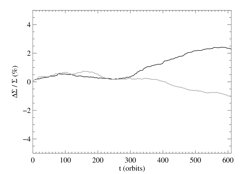
Figure 1.— Variation (in percent) of surface mass density as a function of time $(\Sigma(t)-\Sigma(t=0))/\Sigma(t=0)$ in 1112a(black) and 1126b(gray).

We must also ensure that the MRI is well-resolved throughout the box at all times. The fastest growing mode has a vertical wavevector and wavelength $\lambda_{*}=6.49/\Omega\sqrt{B_{z}^{2}/\rho}$. Averaging $\lambda_{*}$ over horizontal planes, we show the number of grid-cells per wavelength of this mode in Fig. 2. There are at least 8 cells per wavelength (and generally a great many more) everywhere in the box except near the midplane during a few brief epochs (e.g. $T\sim 400$ in 1112a).

The quality of our results also depends on keeping both the top and bottom photospheres within the simulation domain at all times. Fig. 2 also shows the locations of the photospheres in both simulations; we define the photosphere by the place where the Eddington factor $f(\bar{R})=0.5$, for $\bar{R}$ the horizontally-averaged dimensionless opacity parameter. The photospheres are comfortably within the computational domain throughout the duration of both simulations.

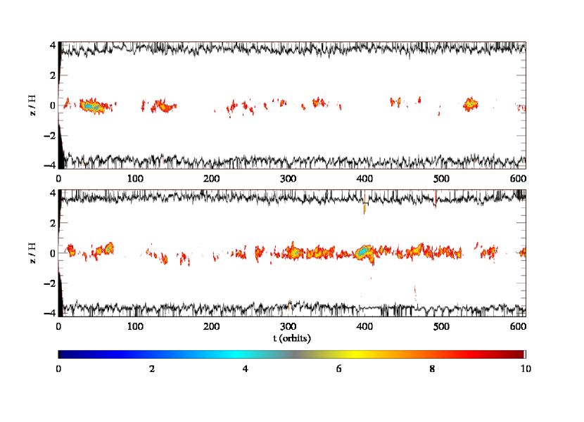
Figure 2.— Top panel: Number of cells per wave length of the most unstable mode of MRI in a horizontally averaged sense (color) and time variation of the photosphere location defined as the Eddington factor $f=0.5$ (solid curves) in 1126b. Bottom panel: Same as the top panel except for 1112a.

3.2. Thermal Balance

The thermal history of the two simulations is shown in Figs. 3 and 4. The top panel in each figure shows the volume integrated dissipation rate per unit surface area of the box (red) and the total radiative flux leaving the top and bottom faces of the box (blue), both on a linear scale. This panel shows clearly that the box is able to maintain a close thermal balance on timescales very short compared to the durations of these simulations. The bottom panels show the total radiation, gas internal, magnetic, and turbulent kinetic energies in the box on a logarithmic scale to emphasize better the relative fluctuations in each of these quantities. If we define the unit of energy content as the gas thermal energy and consider both simulations together, the radiation energy can range from $\simeq 5$–30, the magnetic energy from $\simeq 0.15$–1, and the kinetic energy from $\simeq 0.05$–0.25. Adopting a nominal radiative efficiency of 0.1, we find that the mean stress in simulation 1112a would drive an accretion rate relative to Eddington of 0.17, while in 1126b it would have been 0.23. Thus, even when averaging over relatively long timescales, the mean accretion rate for this surface density and orbital frequency is still uncertain at the level of several tens of percent.

A number of interesting results are apparent in these figures, but the one that is most significant is the fact that an approximate thermal equilibrium has been established in both simulations. The thermal time as measured by the radiation and gas internal energies divided by the total radiative flux has short time scale fluctuations, but averaging over timescales $\sim 50$ orbits, we find that in both simulations the instantaneous cooling time can be anywhere from $\simeq 10$ orbits at times of relatively low energy content to $\simeq 20$ orbits at times of especially high energy in the box. Averaged over the entire duration, the cooling time is 13 orbits in 1112a, and slightly longer, 15.5 orbits, in 1126b. Thus, both simulations ran for $\simeq 40$ thermal times, and yet there is no evidence of runaway heating and cooling. Shakura & Sunyaev (1976) predicted that thermal instability should occur whenever the ratio of radiation to gas pressure exceeds 3/2, but the radiation to gas energy ratios encountered here translate to pressure ratios $\sim 2.5$–15, well above the predicted instability threshold.

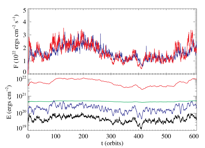
Figure 3.— Top panel: Total volume integrated dissipation (red) and radiative cooling (blue) rates as a function of time in simulation 1112a, plotted on a linear vertical scale. Bottom panel: Total energy content in the box as a function of time in simulation 1112a, in the form of radiation energy (red), gas internal energy (green), magnetic energy (blue), and turbulent kinetic energy (black). (The turbulent kinetic energy is defined as the kinetic energy associated with the fluid velocity measured relative to the background shear flow.) Note that the bottom panel is plotted on a logarithmic vertical scale.

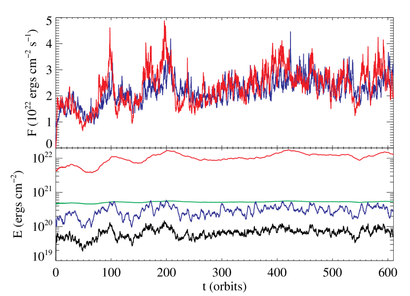
Figure 4.— Same as Fig. 3, except for simulation 1126b.

Although it does appear that a crude long-term mean value for the energy content can be estimated, the amplitude of fluctuations on timescales a significant fraction of the simulation duration is still quite large. We quantify these fluctuations by several measures.

First, we note that transients associated with the initial condition are generally erased by $\simeq 100$ orbits into the simulation. Discounting that initial period, we see that the typical fluctuation amplitudes in the radiation, magnetic, and kinetic energy are similar, all factors of several, but the fluctuation levels in the gas energy are much smaller, only $6\%$ rms. This means that the dissipated magnetic and kinetic energies are readily converted to radiation energy. On the other hand, although there is considerable high-frequency power in the magnetic and kinetic energy fluctuations, there is much less in the radiation energy. That this should be so is not surprising: the turbulence driving the magnetic and kinetic energy densities has a characteristic timescale of order an orbit, whereas the radiation energy changes on a thermal timescale, an order of magnitude longer.

These remarks can be quantified by studying the power spectra of the fluctuations (Fig. 5 illustrates the case of 1112a; 1126b is qualitatively similar). The offset between the magnetic and radiation Fourier power spectra is a measure of the larger contribution from short timescale fluctuations in the time series of magnetic energy. Only at the very longest timescales does the variance in the radiation energy become similar to that in the magnetic energy (and also at very short timescales, where the fluctuation amplitude is extremely small). More quantitatively, both power spectra can be approximately described by broken power-laws:

$$P(f)\simeq\cases{f^{-1.13,-3.65};f_{\rm break}=0.171&magnetic\cr f^{-2.38,-3.91};f_{\rm break}=0.118&radiation\cr}.$$ (17)

The first number in each exponent is the low-frequency slope; the second number is the high-frequency slope. In both cases, the break occurs at $\simeq 5$–10 orbital periods, about half the thermal timescale. At high frequencies, both power spectra decline quite steeply. On the other hand, at low frequencies, both power spectra are “red” enough that the variance is dominated by the low-frequency cut-off posed by the duration of the simulation. This “infrared divergence” is weak—almost logarithmic—for the magnetic fluctuations, but is rather stronger for the radiation spectrum. As we will argue in § 4, the significant power at very long timescales in the magnetic fluctuations is an important element in explaining these disk segments’ thermal stability. As we will also argue, the fact that the two power spectra approach one another at the lowest frequencies is a symptom of the fact that MHD turbulence drives both, so that they must approximately coincide on timescales longer than the thermal equilibration time.

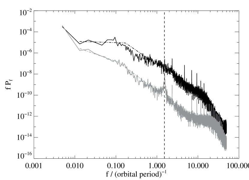
Figure 5.— Variability power spectral densities of volume-integrated magnetic energy (black) and radiation energy (gray) in simulation 1112a. Both time-dependent energies were normalized by their time-averaged values before computing the power spectral densities, and both power spectra are plotted after having been multiplied by the frequency. The vertical dashed curve indicates the expected frequency of the longest wavelength vertical acoustic wave. Dot-dashed curves are broken power law fits to the two power spectra in the frequency range 0.01 to 10.0, scaled by inverse orbital periods.

The essence of the $\alpha$ model is the expectation that the stress should be proportional to pressure. We examine the validity of this expectation in Fig. 6, but using the box-integrated magnetic energy as a stand-in for the stress. As this figure shows, the two do tend to vary together, but with order unity fluctuations about the trend. The logarithmic slope of the least squares fit shown in the figure is 0.71, indicating that the relation is shallower than linear. For future reference (this relationship will be called upon in § 4), we also display (Fig. 7) the analogous relationship between $t_{\rm cool}$ and the integrated radiation energy. The logarithmic slope of the fit in that case is 0.32. It is worth pointing out that the slopes of these relations are subject to some chaotic variation: the magnetic–radiation energy correlation has slope 0.79 and the thermal time–radiation energy correlation has slope 0.44 in simulation 1126b.

Figure 6.— Box-integrated magnetic energy and radiation energy compared every 0.01 orbit from $T=100$ to $T=600$ in simulation 1112a. Both energies are in units of $10^{20}$ erg cm^-3. The dashed line is a least squares fit in the logarithms of these two quantities.

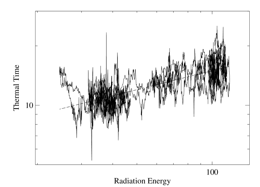
Figure 7.— Thermal time (in units of orbits) and radiation energy (in units of $10^{20}$ erg cm^-3) compared every 0.01 orbit from $T=100$ to $T=600$ in simulation 1112a. The dashed line is a least squares fit in the logarithms of these two quantities.

Casual study of Figs. 3, 4, and 6 suggests that, after allowance for the smoother variations in the radiation energy, all the contributions to the energy content are well-correlated in time. This is almost true. A cross-correlation between them (Fig. 8) reveals, however, that fluctuations in the magnetic energy lead those in the radiation energy (and those in the gas energy) by 5–15 orbits, roughly a thermal time. In § 4, we will show that this fact is a crucial clue for understanding the boxes’ thermal stability. The turbulent kinetic energy, on the other hand (and unsurprisingly) is closely coincident in time with the turbulent magnetic energy.

Figure 8.— Cross correlation with volume integrated magnetic energy of volume integrated radiation energy (solid), gas internal energy (dotted), and turbulent kinetic energy (dashed) as a function of time lag for simulation 1112a. Negative lag implies that the energy in question lags behind the magnetic energy.

We close this subsection by remarking on the quasi-periodic oscillation (QPO) that appears in the power spectrum of radiation energy at a frequency slightly higher than the orbital frequency. We believe this to be a vertical acoustic oscillation. Standing vertical acoustic waves in a polytropic, Newtonian, Keplerian disk can occur at angular frequencies given by

$$\omega=\Omega\left[{n_{z}(n_{z}+2n-1)\over 2n}\right]^{1/2}$$ (18)

where $n_{z}$ is an integer greater than or equal to two and $n$ is the polytropic index (Kato, 2005; Blaes, Arras, & Fragile, 2006). The lowest frequency of this spectrum, $n_{z}=2$, fits the QPO exactly for a radiation pressure supported configuration ($n=3$). The eigenfunction of this mode takes the form of a vertical breathing mode, with fluid displacements expanding and contracting symmetrically about a node at the midplane. As we discuss in section 3.4 below, this mode plays an important role in reconciling the actual vertical profiles of turbulent stress and dissipation with the constraints of thermal and hydrostatic equilibrium.

3.3. Stress

In the original form of the $\alpha$-model, it is supposed that the stress bears a fixed ratio to the total pressure. However, it has also been proposed (Sakimoto & Coroniti, 1981; Taam & Lin, 1984), usually with a view toward quenching the thermal instability, that the stress might instead scale more closely with the gas pressure alone, or with the geometric mean of the gas and radiation pressures. We can test these hypotheses with our simulation data.

Fig. 9 shows the time dependence of the box average of the $r\phi$ component of the Maxwell and turbulent Reynolds stress in simulation 1112a. The fact that it has considerable short timescale fluctuation power immediately rules out the possibility that it should respond to either the gas pressure or the radiation pressure in all respects because their histories show only very weak short timescale fluctuations. The large amplitude fluctuations in the stress over long timescales similarly show that it cannot be driven, even in an averaged sense, by the gas pressure, for the fluctuations in the gas pressure are far too small. That the volume-averaged stress is at all times well below the critical stress for pure radiation support demonstrates that, although radiation pressure truly dominates in the central part of the disk, other mechanisms (notably magnetic pressure, as we will show in § 3.4) account for support against vertical gravity in substantial portions of the total simulation volume.

Figure 9.— Time dependence of the box-averaged $r\phi$ stress in simulation 1112a. The horizontal dashed line indicates the $2c\Omega/3\kappa$ stress expected from hydrostatic and radiative equilibrium.

To make this point very explicit, we show in Fig. 10 the time-dependence of the ratio of the box-integrated stress to the different box-integrated candidate pressure quantities for simulation 1112a. That is, these curves show the time-dependent Shakura-Sunyaev $\alpha$ parameter for various stress prescriptions. The best would presumably be the one that gives a value of $\alpha$ that varies least with time. The least variation (taking the stress divided by the gas plus radiation pressure) is a factor of 4, while the greatest variation (found when the stress is measured in units of the gas pressure) is a factor of 10. In no case, therefore, does the stress follow exactly the fluctuations in any of these pressure measures.

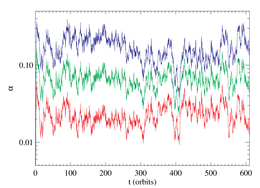
Figure 10.— Time dependence of the ratio $\alpha$ of the box-averaged $r\phi$ stress to various box-averaged pressures in simulation 1112a. From top to bottom, the stress is scaled with gas pressure, the geometric mean of gas and radiation pressures, and with total (gas plus radiation) pressure, respectively.

It is worth remarking in this context that the mean value of the ratio of integrated stress to integrated total pressure was 0.023 in 1112a and 0.019 in 1126b. In our previous simulations, this number was $\simeq 0.03$ (for the $p_{r}\sim p_{g}$ simulation reported in Krolik, Hirose, & Blaes (2007)) and 0.016 (for the $p_{r}/p_{g}\simeq 0.2$ simulation of Hirose, Krolik, & Stone (2006)). Thus, we see little trend in this ratio as a function of the ratio of radiation to gas pressure. In addition, this series of simulations is, somewhat inadvertently, a crude test of numerical convergence. Due both to the requirements of the simulations and to the increase in available computational power over time, the resolutions employed have improved steadily from one to the next. Measured in terms of our estimated scale-height, the cell-size $\Delta z$ changed from $0.0625H$ in the gas-dominated simulation to $0.0234H$ in the $p_{r}\sim p_{g}$ simulation to $0.0094H$ in the simulations presented here. The rough constancy of the stress/pressure ratio across these simulations is of some interest in view of reports that unstratified shearing box simulations show a declining ratio of stress to pressure as resolution improves (Fromang & Papaloizou, 2007). It should be pointed out, however, that these unstratified simulations had zero net magnetic flux, whereas our stratified simulations have a net azimuthal flux, albeit one that is not preserved by the boundary conditions and fluctuates in direction over the course of the simulations.

3.4. Vertical Energy Transport and Hydrostatic Balance

As first pointed out by Shakura & Sunyaev (1976), in any radiation-dominated geometrically-thin disk, there is a characteristic emissivity per unit volume: $j_{*}=c\Omega^{2}/\kappa$. Its existence follows immediately from attributing hydrostatic balance to radiation force. When that condition is met (and the opacity is purely electron scattering),

$$\kappa_{\rm es}{F_{z}}/c=z\Omega^{2};$$ (19)

differentiating both sides with respect to height $z$ gives

$${\kappa_{\rm es}\over c}{d{F_{z}}\over dz}\equiv{\kappa_{\rm es}\over c}j=\Omega^{2}.$$ (20)

If all the dissipation is transformed locally into photon energy, there is a corresponding characteristic dissipation rate $Q_{*}=j_{*}$. We find (Fig. 11) that the dissipation rate is comparable to $Q_{*}$ through most of the disk body, but is typically somewhat greater at $|z|\simeq 0.5H$ (by $\simeq 30\%$) and rather less in the upper disk. At all altitudes it is dominated by magnetic losses.

If hydrostatic balance obtains (as we will show shortly, departures are almost always small), where $Q>Q_{*}$ over a significant range in height, it must be that $j<Q$ because otherwise the flux would exceed the value whose force balances gravity. Consequently, not all the energy liberated by dissipation goes directly into radiation flux. As shown in Fig. 12, for $|z|\lesssim 2H$, a noticeable (but minority: $\sim 10\%$) fraction of the vertical energy flux is in the form of photons advected upward with the matter ($Ev_{z}$), rather than diffusing through it ($F_{z}$); because this component does not move through the matter, it exerts no force. Like the total radiation content in the box, the advective energy flux also oscillates with the frequency of the fundamental vertical breathing mode. If this oscillation behaved with exact symmetry in its outward and inward moving phases, it would carry no net energy. However, at the outer surface of the region of significant advection ($|z|\simeq 2H$), we see a divergence of the diffusive flux that exceeds the local dissipation rate (Fig. 13); that is, radiation energy diffuses out of the upwelling matter at the top of its oscillatory range. In this respect, the radiative advection seen here resembles convection, although the vertical gas motions are acoustic in nature and not due to buoyancy. In addition, a smaller amount of energy is carried upward by work done by radiation pressure forces and by Poynting flux $(\bm{E}\times\bm{B})_{z}$, which also oscillates with the frequency of the breathing mode. Clearly, MHD flux-freezing causes magnetic energy to be advected with the gas along with radiation energy in the breathing mode. The energy transported by radiation advection, work done by radiation pressure, and Poynting flux is deposited (or dissipated) around $H\lesssim|z|\lesssim 2H$. Above this point, the energy flux is overwhelmingly due to radiation diffusion. Energy transport by gas advection $(e+\rho\bm{v}^{2}/2)v_{z}$ and gas pressure work is negligible throughout the simulation domain.

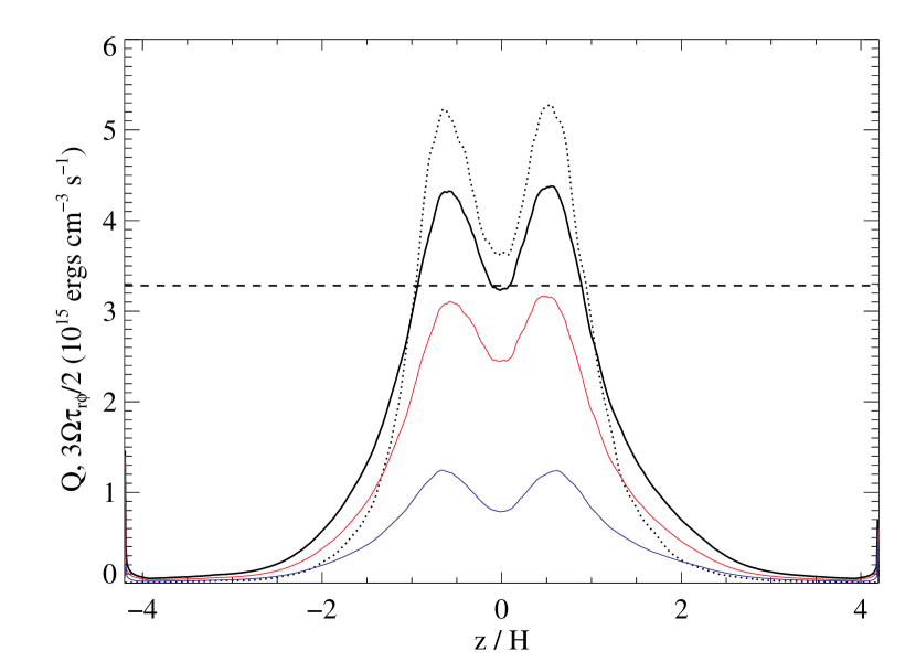
Figure 11.— Horizontally and time-averaged total dissipation rate $Q$ (black) and stress times rate of strain (dotted) in simulation 1112a. The total dissipation rate is the sum of magnetic energy dissipation (red) and kinetic energy dissipation (blue). The horizontal dashed line marks the characteristic dissipation rate $Q_{*}=c\Omega^{2}/\kappa$.

Fig. 11 also shows the vertical profile of stress times rate of strain, $-\tau_{r\phi}d\Omega/d\ln r$. This profile is significantly more concentrated near the midplane and at $z=\pm 0.5H$ than the dissipation profile, indicating that the work done by the turbulent stresses is, in the time average, partly dissipated locally and partly converted into mechanical energy of gas motion, which is then transported vertically primarily by Poynting flux and radiation pressure work associated with the breathing mode and dissipated farther out. This energy is deposited well outside the peak region of stress, and subsequently carried further outward by radiative diffusion. This supplemental energy transport mechanism contributes to $dF_{z}/dz$, helping to maintain radiation-aided support against gravity at altitudes higher than one might expect if dissipation correlated perfectly with local stress.

The net result of these processes is illustrated most clearly in Fig. 13. As this figure shows, despite the peaks in $Q$ that reach well above $Q_{*}$, the divergence of the radiation flux $F_{z}$ is kept just under $j_{*}$ across the entire central body of the disk, from $z\simeq-1.5H$ to $z\simeq+1.5H$. It is the radiation advection flux $Ev_{z}$ that compensates for the excess dissipated energy $(Q-Q_{*})$ and carries it away. Thus, thermal balance is locally maintained in the entire region, as evidenced by the fact that the divergence of the summed radiation and gas energy fluxes ($F_{z}+Ev_{z}$) matches the dissipation rate $Q$ very well. At the same time, Poynting flux $(\bm{E}\times\bm{B})_{z}$ and the flux of work done by radiation pressure forces transports non-dissipated excess mechanical energy away from the midplane to be dissipated further out. The sum of the divergences of all these energy fluxes (together with advection of gas energy and work done by gas pressure, which are both small) compensates exactly for the work done on the fluid by turbulent stresses, thereby establishing global energy conservation.

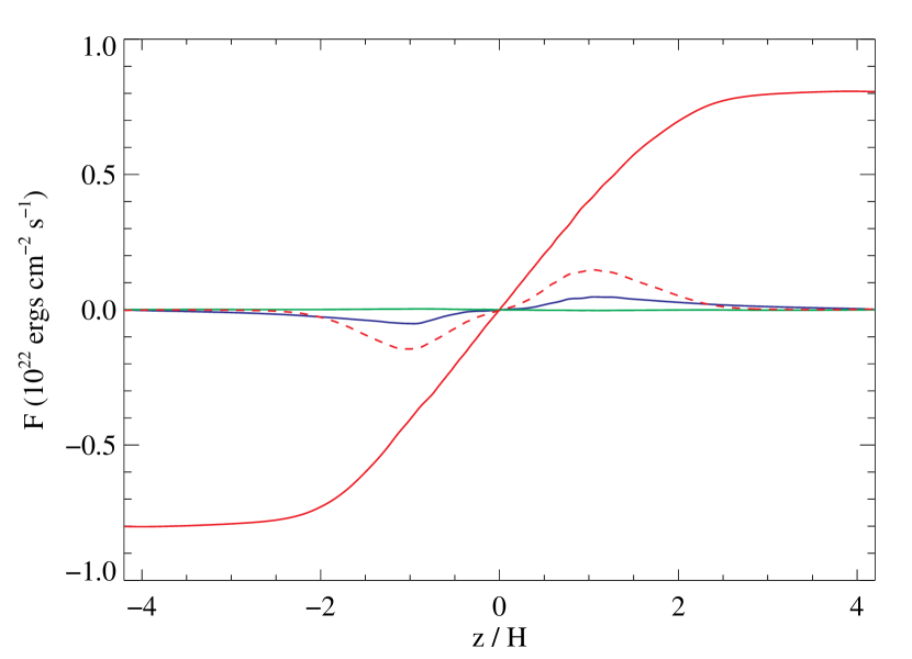
Figure 12.— Horizontally and time-averaged diffusive radiation energy flux $F_{z}$ (solid red), advected radiation energy flux $Ev_{z}$ (dashed red), Poynting flux $(\bm{E}\times\bm{B})_{z}$ (blue), and advected gas energy flux $(e+\rho\bm{v}^{2}/2)v_{z}$ (green) in simulation 1112a.

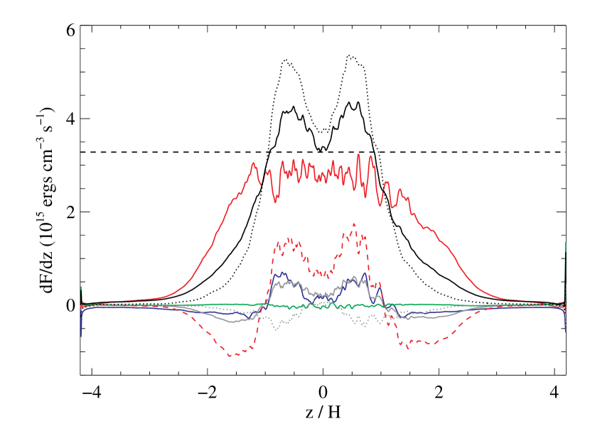
Figure 13.— Horizontally and time-averaged vertical derivatives of diffusive radiation energy flux $F_{z}$ (solid red), advected radiation energy flux $Ev_{z}$ (dashed red), Poynting flux $(\bm{E}\times\bm{B})_{z}$ (blue), and advected gas energy flux $(e+\rho\bm{v}^{2}/2)v_{z}$ (green) in simulation 1112a. In addition, the grey curve shows the profile of $\mathsf{P}:\nabla\bm{v}-\chi\rho\bm{F}\cdot\bm{v}/c$, which is equivalent to the divergence of the flux $Ev_{z}/3$ of work done by radiation pressure when the medium is optically thick. The sum of the diffusive and advective radiation energy flux derivatives is shown as the solid black line, and matches well the horizontally and time-averaged dissipation profile $Q$ (solid black line in Fig. 11). The sum of all the flux derivative profiles is shown as the dotted black line, and matches well the horizontally and time-averaged profile of stress times rate of strain (dotted black line in Fig. 11). For reference, the horizontal dashed line marks the characteristic dissipation rate $Q_{*}=c\Omega^{2}/\kappa$.

Consistent with the rough match between $Q$ and $Q_{*}$, most of the vertical support, particularly in the center of the disk, is due to radiation forces (Fig. 14) and hydrostatic balance is maintained quite closely. In fact, departures from time-averaged hydrostatic balance are smaller, in fractional terms, than any local deviation (again time-averaged) between $Q$ and $Q_{*}$. In general terms, this occurs because the timescale for dynamical equilibration ($\sim 1/\Omega$) is the shortest timescale in the system. In detail, two different effects account for the fact that deviations from hydrostatic balance are so small. As just discussed, in the disk body, where $Q>Q_{*}$, some of the vertical energy transport is carried by other mechanisms, notably radiation advection (Fig. 12). At higher altitudes, vertical support depends more on the gradient of magnetic pressure than on the gradient of radiation pressure.

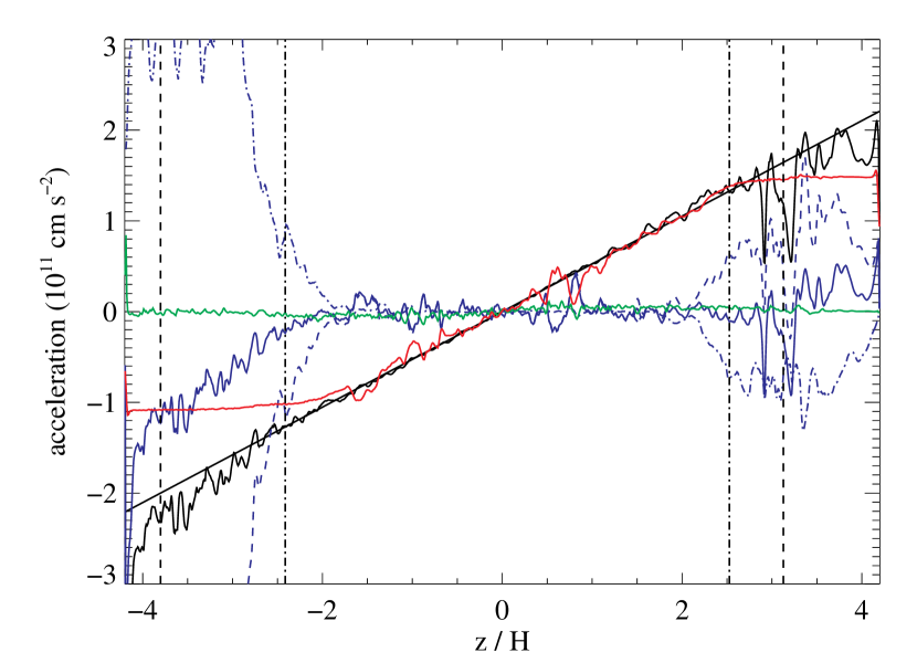
Figure 14.— Horizontally averaged vertical accelerations at the 200 orbits epoch in simulation 1112a. The different curves show accelerations from radiation pressure (red), gas pressure (green), and magnetic forces (blue). The total of these accelerations is the black curve, and is comparable to the straight black line indicating the gravitational acceleration. The dashed blue curve is the contribution to the magnetic acceleration from magnetic pressure gradients, while the dot-dashed blue curve indicates the contribution from magnetic tension. The vertical dashed and dot-dashed lines indicate the locations of the scattering and thermalization photospheres of the horizontally-averaged structure, respectively.

The structure that is established by these several forces is very similar qualitatively to the structure seen in all previous vertically-stratified shearing-box simulations with genuine thermodynamics: a central region ($|z|<3H$) supported by a combination of gas and radiation pressure lying within an outer region dominated by magnetic forces. Within the magnetically-dominated region, the outward force due to the magnetic pressure gradient is substantially cancelled (in the mean) by the inward force due to magnetic tension (Fig. 14).

The resulting profiles of density and pressure are roughly exponential (Figs. 15 and 16). An exponential description is particularly good for the density, with time-averaged scale-height $\simeq 0.8H$. However, we caution that the instantaneous scale-height can vary by order unity as the radiation energy varies up and down. It is also appropriate to remark at this point that, contrary to the simple assumption made in classical $\alpha$-models, the density is very far from constant because the dissipation per unit mass is also very far from constant. As we have found in earlier vertically-stratified studies with smaller ratios of radiation to gas pressure, the dissipation rate per unit mass increases with decreasing mass column density to the nearest outer surface.

Figure 15.— Horizontally and time-averaged vertical density profile in the 1112a (solid) and 1126b (dashed) simulations.

The pressures, while still behaving roughly as exponentials in height, have additional structure. The radiation pressure declines more steeply within $|z|<3H$ than without because the density drops so steeply outward. From the photosphere outward, the radiation pressure changes only slowly with height because that is the free-streaming limit in plane-parallel geometry. The magnetic pressure profile, on the other hand, is roughly flat-topped in the central disk, with a pair of weak local maxima at $|z|\simeq H$. In that central region, the plasma $\beta\simeq 50$, but it drops rapidly outward, falling below unity at $|z|\simeq 2.5H$ where the magnetic pressure begins to dominate the total.

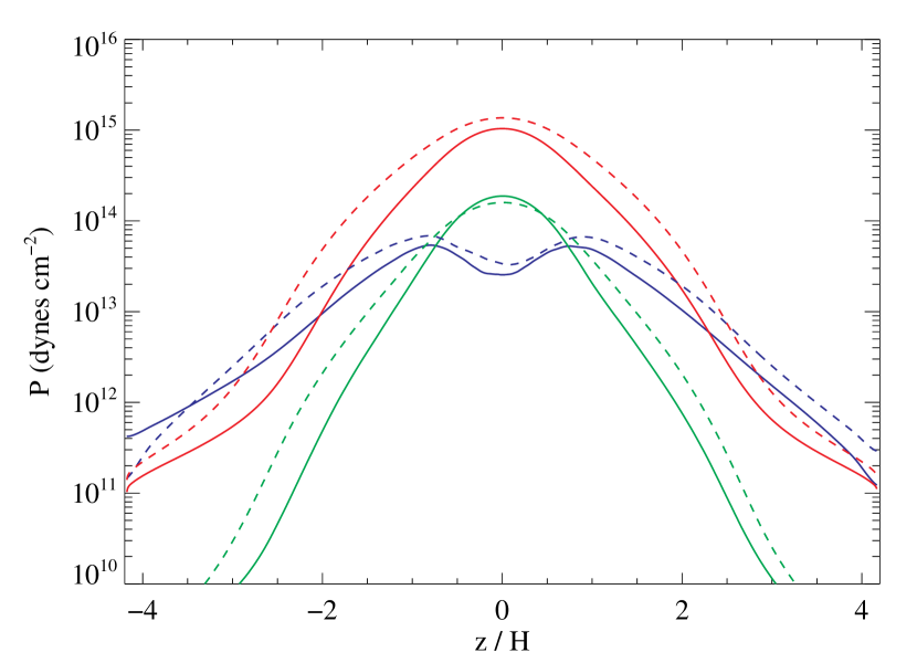
Figure 16.— Horizontally and time-averaged vertical profiles of radiation pressure (red), gas pressure (green) and magnetic pressure (blue) in the 1112a (solid) and 1126b (dashed) simulations.

Fig. 17 shows horizontally and time-averaged gas temperature $T$ and radiation temperature $T_{\rm rad}\equiv(E/a)^{1/4}$, while Fig. 18 shows the height of the scattering and thermalization photospheres as functions of time for simulation 1112a. These photospheres are defined as the surfaces where the horizontally averaged scattering optical depth and geometric mean of the scattering and Planck mean absorption optical depths, respectively, equal unity. The time-averaged height of the thermalization photosphere in simulation 1112a was $2.0H$, in approximate agreement with the height at which the time-averaged gas and radiation temperatures begin to separate in Fig. 17. The scattering photosphere is of course further out, with a time-averaged height of $3.3H$.

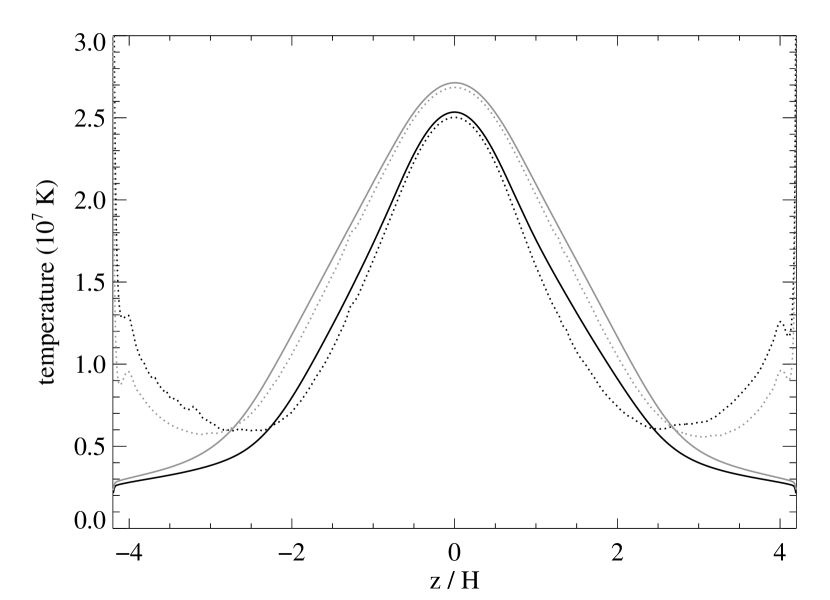
Figure 17.— Horizontally and time-averaged gas temperature (solid) and radiation temperature (dotted) in 1112a (black) and 1126b (gray).

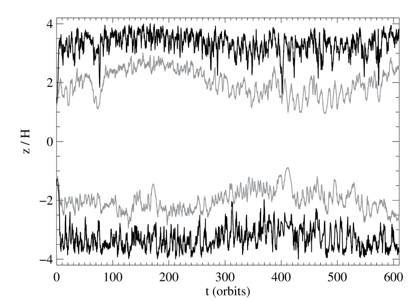
Figure 18.— Horizontally-averaged height of the scattering (black) and thermalization (gray) photospheres as functions of time in 1112a.

Fig. 19 shows that very large density fluctuations are always present at both the thermalization and scattering photospheres of the horizontally averaged structure. Similarly large density fluctuations in the photospheres have been seen in all our previous simulations (see Fig. 16 in Blaes, Hirose, & Krolik 2007), and are due to the fluctuating magnetic forces that dominate all other forces in these regions.

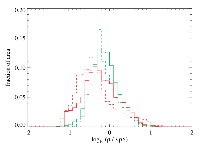
Figure 19.— Histogram of the ratio of density to horizontally-averaged density at the thermalization (green) and scattering (red) photospheres of the horizontally averaged structure at epoch 200 in simulation 1112a. The upper and lower photospheres are indicated by solid and dashed histograms, respectively. The fluid motions are highly compressible in this region due to the large ambient magnetic forces.

We close this section by remarking that we have confirmed many of the results seen in the radiation pressure dominated simulation of Turner (2004), despite the fact that that simulation was not fully energy conserving, nor did it include the photospheres within the simulation domain. In particular, he also found no thermal instability and a vertical density profile that was highly concentrated toward the midplane. As shown in Fig. 20, we also find similarly small density fluctuations near the midplane, of at most a factor $\sim 2$ between maximum and minimum. The magnetic pressure profile in his simulation had a double-peaked structure that was lower than the gas pressure at the midplane, but exceeded the gas pressure further out, also in agreement with what we have found. However, his magnetic pressure nowhere exceeded the radiation pressure, in contrast to the outermost layers in our simulation. Moreover, he found that radiative diffusion carried only two-thirds of the outward energy flux, with radiation advection being the most important secondary coolant. These differences can perhaps be ascribed to the fact that his simulation did not include the photospheres. If we neglected the data from our simulations outside $|z|=2H$, we would see results qualitatively similar to his.

The only respect in which we really disagree is that Turner (2004) also claimed that radiation damping (Agol & Krolik, 1998) contributed $29\%$ of the heating in the midplane regions of his simulation. However, we have demonstrated a complete accounting of the thermal energy balance without calculating the contribution from this process at all. Turner computed the radiation damping rate by integrating $-P\nabla\cdot\bm{v}$ over the midplane region of his box, with $P=E/3$ where radiation dominates and is isotropic. This is a reasonable method in a nonstratified shearing box (Turner, Stone & Sano, 2002) because the volume is fixed: consequently, the net compressive work indicates non-adiabatic behavior. However, in a stratified shearing box, $P\nabla\cdot\bm{v}$ is really a piece of the divergence of the flux of work done by radiation pressure, $\nabla\cdot(P\bm{v})$, and we have shown that this plays a contributing role to transporting excess mechanical energy out of the midplane by the breathing mode to be dissipated further out. Moreover, even if we follow Turner in using $-P\nabla\cdot\bm{v}$ to provide an estimate of the radiation damping near the midplane, we then find that this can be at most $1.3\%$ and $0.7\%$ percent of the dissipation in the midplane region in 1112a and 1126b, respectively. It is conceivable that one of two limitations in Turner’s code may be responsible for this quantitative difference between his simulation and ours: the lack of a photosphere and the inability to capture grid scale losses of kinetic energy. Without performing additional simulations that separately reproduce each of these possibilities, we cannot be certain as to the exact origin of the discrepancy. Nevertheless, we suspect that lack of true energy conservation in Turner’s simulation is the primary cause.

Figure 20.— Histogram of the ratio of density to horizontally-averaged density at the midplane for simulation 1112a at epoch 200. The fluid motions are highly incompressible in this region.

4. Interpretation

In the traditional $\alpha$-model approach, whose logical underpinning is dimensional analysis, the stress, and therefore the magnetic field energy density, is scaled to the pressure. Considered in a logically rigorous fashion, dimensional analysis suggests that two quantities with the same units are comparable in magnitude, but does not determine a causal relation between the two: that is, it does not tell us which quantity determines the other. Nonetheless, if it is easier to estimate one than the other, it is easy to slip into the thought that the one harder to estimate follows the other, not just in scale, but in time. In this case, the $\alpha$-model has often been imagined to suggest that the pressure controls the magnetic field.

However, a crosscorrelation of the magnetic field energy against the radiation energy in this simulation shows that fluctuations in the magnetic field lead those in the radiation. If so, the dominant sense of causality must be the other way around—the magnetic field controls the radiation, not vice versa. In fact, that is the direction suggested by the dynamics: The MRI causes field fluctuations to grow, deriving the needed energy from orbital shear; nonlinear mode-mode interactions move power from long lengthscales to short; short wavelength dissipative effects transfer energy from the magnetic field to heat in the plasma; finally, electrons in the plasma radiate photons. In other words, intrinsic fluctuations in the magnetic turbulence can create a pressure-stress correlation even when there is no direct influence of the pressure on the saturation level of the magnetic field. All that is required is that their amplitude on timescales long compared to a thermal equilibration time are large enough, and these are already known to occur even in gas-dominated cases in which the pressure varies very little (Hirose, Krolik, & Stone, 2006). When that is the case, the increased dissipation rate due to the stronger field leads to higher pressure, but not necessarily to any subsequent increase in the stress. Thus, a key assumption of the argument for thermal instability in the radiation-dominated regime is undermined.

Using an approach reminiscent of the long-wavelength limit of the formalism developed in Piran (1978), the qualitative picture outlined above can be modelled by the following pair of equations:

$$\frac{dE_{B}}{dt} = R(t){E_{B0}\over t_{\rm growth}}\left(\frac{E_{R}}{E_{R0}}\right)^{n}-{E_{B}\over t_{\rm diss}}$$ (21)

$$\frac{dE_{R}}{dt} = {E_{B}\over t_{\rm diss}}-{E_{R}\over t_{\rm cool}},$$ (22)

where $E_{B,R}$ are the box-integrated magnetic and radiation energies, $E_{B0,R0}$ are their equilibrium values, and $R(t)$ is a random function with expectation value unity describing the intrinsic fluctuations in the scaling of magnetic energy density with pressure. We also suppose that the equilibrium magnetic energy density grows with pressure (here the radiation energy) with logarithmic derivative $n$. Thus, we allow for feedback in the sense that the pressure might be able to influence the stress. Lastly, $t_{\rm growth}$ is the timescale for the magnetic energy to adjust toward its expectation value, $t_{\rm diss}$ is the timescale for magnetic dissipation, and $t_{\rm cool}$ is the radiation cooling time. The magnetic field energy matches the equilibrium value when $t_{\rm growth}=t_{\rm diss}$, so these two timescales may be equated. Non-dimensionalizing the energies in terms of their equilibrium values and the time in terms of $t_{\rm diss}$, these equations become

$$\frac{d{\cal E}_{B}}{d\tau} = R(t){\cal E}_{R}^{n}-{\cal E}_{B}$$ (23)

$$\frac{d{\cal E}_{R}}{d\tau} = {\cal E}_{B}\frac{E_{B0}}{E_{R0}}-\frac{t_{\rm diss}}{t_{\rm cool}}{\cal E}_{R}.$$ (24)

The timescale ratio $t_{\rm diss}/t_{\rm cool}$ may also depend on pressure; we designate its logarithmic derivative with respect to pressure by $-s$ (the minus sign makes its definition consistent with the notation in Krolik, Hirose, & Blaes (2007)).

That assumption puts the model equations in the form:

$$\frac{d{\cal E}_{B}}{d\tau} = R(t){\cal E}_{R}^{n}-{\cal E}_{B}$$ (25)

$$\frac{d{\cal E}_{R}}{d\tau} = {\cal E}_{B}\frac{E_{B0}}{E_{R0}}-\frac{t_{\rm diss,0}}{t_{\rm cool,0}}{\cal E}_{R}^{1-s}.$$ (26)

Once again we can use the requirement that equilibrium values be consistent with zero time-dependence to constrain these parameters: this time we conclude that $t_{\rm diss,0}/t_{\rm cool,0}=E_{B0}/E_{R0}$, leaving

$$\frac{d{\cal E}_{B}}{d\tau} = R(t){\cal E}_{R}^{n}-{\cal E}_{B}$$ (27)

$$\frac{d{\cal E}_{R}}{d\tau} = \frac{E_{B0}}{E_{R0}}\left[{\cal E}_{B}-{\cal E}_{R}^{1-s}\right].$$ (28)

In other words, the timescale for the radiation energy to equilibrate is $\sim E_{R0}/E_{B0}$ times the timescale on which the magnetic energy can fluctuate; the magnetic energy must be dissipated many times over in order to produce a response in the radiation energy because $E_{R0}/E_{B0}$ is so large. For context, we recall that in the simulations described here, the mean $E_{R}/E_{B}\simeq 30$ while the mean thermal timescale was $\simeq 15$ orbits. If this toy-model describes the simulations, i.e., if heating in the simulations is primarily due to magnetic dissipation and cooling is due to radiation losses, these numbers would suggest that in the simulations $t_{\rm diss}$ should be defined as the ratio of box-integrated magnetic energy to magnetic dissipation rate, and its typical value should be $\simeq 0.5$ orbits. In fact, consistent with this description of energy balance, the mean value of $t_{\rm diss}$ defined in this way was 0.53 orbits in simulation 1112a, and 0.55 orbits in simulation 1126b.

In Fig. 21, we show a sample solution of these equations, in this case with $n=s=0$, $E_{B0}/E_{R0}=0.033$, and initial conditions ${\cal E}_{R}={\cal E}_{B}=1$. Note that setting $n=0$ means that there is no explicit dependence of magnetic amplification on the radiation pressure. The random function $R(t)$ was constructed by requiring its power spectrum to match approximately the power spectrum of magnetic energy fluctuations seen in simulation 1112a (i.e., $\propto f^{-1.13}$ at frequencies $f\leq 2.6/t_{\rm cool}$ and $\propto f^{-3.65}$ for $f>2.6/t_{\rm cool}$), but choosing the phases of its Fourier amplitudes randomly with uniform probability distribution in the interval $[0,2\pi)$. To make the comparision as direct as possible, the duration of the integration was set to $40t_{\rm cool}$. Just as in the simulations, the radiation energy fluctuates by factors of several over this timespan, but shows no clear trend.

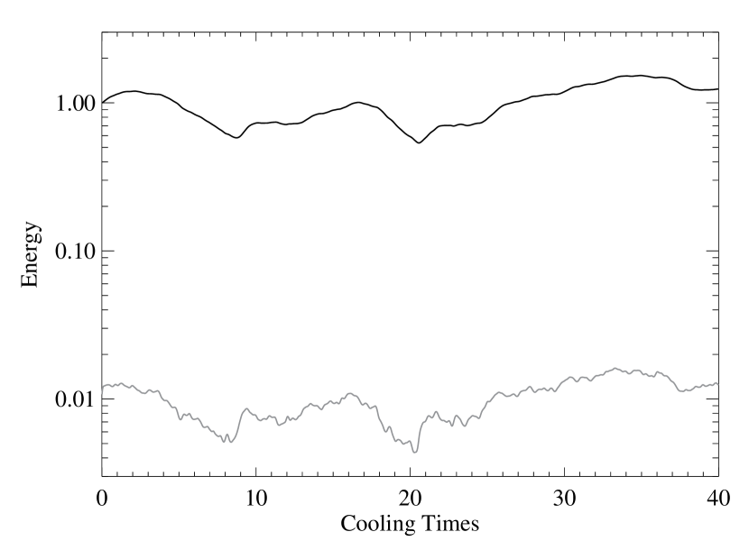
Figure 21.— Radiation energy (black curve) and magnetic energy (gray curve) as functions of time in units of $t_{\rm cool}$, as computed on the basis of the toy-model described in the text.

Guided by a traditional view of the $\alpha$ model, one might object that the absence of thermal instability here is due to the lack of any explicit dependence of the magnetic energy on the radiation energy. However, closer study of the differential equations suggests that if $t_{\rm cool}$ is short compared to the timescale of the large-amplitude turbulence fluctuations, approximate radiative equilibrium is enforced on the shorter timescale. It would then follow that ${\cal E}_{B}\propto{\cal E}_{R}^{1-s}$ independent of $n$. This is exactly what we see, for these parameters and all other combinations of $n$ and $s$ we have tried, subject only to the constraint that $n<1-s$ (as discussed in Krolik, Hirose, & Blaes (2007), genuine instability can be found when this limit is violated). The flat power spectrum at frequencies below $1/t_{\rm cool}$ guarantees that there is substantial fluctuation power on timescales longer than the radiative equilibration timescale, and the result is as predicted, as shown by Fig. 22. A linear least-squares fit in the logarithms of these two quantities then yields a best-fit relation in which $d\log{\cal E}_{B}/d\log{\cal E}_{R}\simeq 1-s$; in the example shown, in which $s=0$, the best-fit logarithmic derivative was 1.01. Thus, magnetic energy and pressure do scale together as suggested by the dimensional analysis underlying the $\alpha$ model, but it is not necessarily because the pressure directly forces the magnetic energy; it is instead the other way around: the pressure is the result of magnetic dissipative heating regulated by photon losses.

Figure 22.— Correlation plot between ${\cal E}_{R}$ and ${\cal E}_{B}$.

We now see the data shown in Fig. 6 in a different light. Although it is true that, compared at the same time, $E_{B}\propto E_{R}^{0.71}$ in that simulation, this correlation is created by the dependence of the radiation energy on the magnetic energy, and not by the radiation pressure regulating the magnetic field strength. Moreover, if our simple model correctly describes the thermal balance, the slope of this correlation should be $1-s$, so that $t_{\rm cool}/t_{\rm diss}\propto E_{R}^{0.29}$. We have already seen that $t_{\rm cool}\propto E_{R}^{0.32}$; a logarithmic least-squares linear fit to the data of 1112a gives $t_{\rm diss}\propto E_{R}^{0.02}$, supporting the toy-model.

An important corollary of these results is that the intrinsic dependence of magnetic energy on radiation pressure parameterized by $n$ cannot be inferred from the slope of the correlation between magnetic energy and radiation energy; this slope is entirely independent of it. The most that one can do is to place an upper bound on how strongly pressure influences magnetic saturation by using the observed thermal stability to argue that $n<1-s$.

To close this section, we make the qualitative remark that the sensitivity of the cooling time to pressure may influence the magnitude of fluctuations in the energy content. As argued in Krolik, Hirose, & Blaes (2007), provided $t_{\rm diss}$ is not too strong a function of box energy content, $s$ must be relatively large in magnitude and negative when gas pressure dominates radiation pressure because an increasing ratio of radiation to gas pressure makes diffusive cooling much more rapid. If so, the cooling time rapidly shortens when the radiation energy increases, placing a tight cap on fluctuations in the energy content of the box. When the radiation to gas pressure ratio is order unity or greater, the scaling of $t_{\rm cool}$ with total energy should be rather slower (a prediction consistent with our results if $t_{\rm diss}$ is likewise not a strong function of $E_{R}$). In this case, the cooling time is comparatively insensitive to energy content and exercises looser control on energy fluctuations, permitting the turbulence fluctuations to drive larger amplitude fluctuations in the total pressure.

5. Conclusions and Summary

In this paper we have presented the results of two simulations that each followed the evolution of a vertically-stratified shearing box with the same surface density and orbital frequency for $\sim 600$ orbits, or $\sim 40$ thermal times. The initial conditions of the two simulations differed only in being given different realizations of the small amplitude noise that was imposed on their otherwise smooth initial state. Because the magneto-rotational instability generates MHD turbulence, these systems are chaotic; differing small amplitude noise therefore leads to order unity contrasts in their subsequent evolution. The two simulations should thus be viewed as two different realizations of the many evolutions possible for these parameters. Their qualitative aspects are, nonetheless, similar.

For example, just as we have found in previous simulations studying shearing boxes with $p_{r}\simeq 0.2p_{g}$ (Hirose, Krolik, & Stone, 2006) and $p_{r}\sim p_{g}$ (Krolik, Hirose, & Blaes, 2007), most of the disk mass is found near the midplane, where the magnetic field energy is $\sim 10^{-2}$ times the combined gas and radiation pressure (see also Turner 2004). Likewise, in all cases the upper layers of the disk are magnetically-dominated, and the photosphere lies within this region. Unlike the earlier simulations, in these two the box-averaged radiation pressure is $\sim 10$ times greater than the gas pressure at all times.

Most importantly, in both cases, the energy content of the box undergoes order unity fluctuations over timescales of many tens of orbits, but these fluctuations have no long-term trend. This result directly challenges the prediction made in Shakura & Sunyaev (1976) that radiation pressure-dominated disk segments should be thermally unstable. Note, however, that the prediction by Lightman & Eardley (1974) of inflow instability in radiation-dominated disks remains to be investigated.

In our simulations, the time-averaged dissipation rate in the disk body is roughly equal to the characteristic value $c\Omega^{2}/\kappa_{\rm es}$, the rate at which diffusive radiation flux maintains hydrostatic balance (Shakura & Sunyaev, 1976). However, in some places ($|z|\sim H$), the local dissipation rate exceeds the characteristic value by more than $30\%$. If this heat went into radiation flux, hydrostatic balance would be disrupted. We find that the excess is exactly compensated by radiative advection associated with an acoustic breathing mode. At the same time, mechanical work done on the fluid by the shearing boundaries in excess of the local dissipation rate is transported outward by Poynting flux and radiation pressure work associated with the breathing mode. Both the dissipated energy carried by radiation advection and (non-dissipated) energy carried by Poynting flux and radiation pressure work are finally deposited and dissipated at $|z|\sim 2H$, and from there all the way through the rest of the structure radiation diffusion overwhelms all other energy fluxes.

To explain the thermal stability of radiation-dominated disks, we argue that the comparability of stress and pressure inferred from dimensional analysis (which underlies the $\alpha$-model, and the prediction of instability) is due to dissipation of magnetic turbulence (which produces the stress) providing the heat that is then transformed into radiation pressure. Consequently, fluctuations in magnetic energy drive fluctuations in pressure, and not (as has been commonly assumed) the other way around. Our claim is supported by two lines of evidence: First, crosscorrelation analysis of simulation data demonstrates that magnetic fluctuations lead radiation energy fluctuations by 5–15 orbits, a little less than a thermal time. Pressure fluctuations cannot, then, drive magnetic fluctuations. Second, we constructed a simple model realizing this picture, and this model reproduces two other important features observed in the simulation data: The system undergoes thermal fluctuations closely resembling in amplitude and timescale those seen in the simulations. In addition, although no correlation between magnetic energy and radiation pressure is built into the model, thermal balance automatically creates one after the fact. Thus, correlations between stress and pressure are due to the dissipation of magnetic energy supplying thermal energy, not to the pressure defining a characteristic scale for the stress.

A logical consequence of this point of view, in which stress determines pressure, rather than the other way around, is that the fundamental independent variables are surface density and orbital frequency. That the orbital frequency is independent of disk parameters is obvious, so long as the disk mass is small compared to the central mass. So long as the inflow timescale is long compared to the thermal timescale, the surface density must likewise be regarded as an independent parameter with respect to thermal and dynamical fluctuations. These two independent parameters, through the intertwined and nonlinear processes of MHD instability, tapping the energy reservoir of orbital shear, magnetic dissipation, thermal radiation, and radiative diffusion, with all of these taking place under conditions of vertical (as well as radial) gravitational confinement, combine to determine the magnetic field strength, both its mean saturation level and its fluctuations. Orbital shear fixes the stress exerted by this field, while the turbulent cascade sets the dissipation rate. These two are not entirely separate, of course, as the time-averaged accretion rate is equivalent to either one. The pressure follows from the heating rate, as regulated by photon diffusion, and, in turn, closes the loop by determining the disk thickness. Despite all these complications, at bottom, everything is still determined by only two variables, surface density and orbital frequency.

We are grateful to Shane Davis, Jim Stone, and Neal Turner for very useful discussions and comments. This work was partially supported by NSF Grant AST-0507455 and NASA ATP Grant NNG06GI68G (JHK) and NSF Grants AST-0307657 and AST-0707624 (OMB). The computations were performed on the SX8 at the Yukawa Institute for Theoretical Physics of Kyoto University and the VPP5000 at the Center for Computational Astrophysics of the National Astronomical Observatory of Japan.

Appendix A Numerical methods for solving the matter-radiation energy exchange equations

To solve the equations for matter energy density $e$ (eqn. 5) and radiation energy density $E$ (eqn. 6), we follow our usual system of operator-splitting. Because energy removed from one of these reservoirs can go directly into the other, we treat the operator-split segments in pairs.

A.1. Free-free absorption

First we group together the work done by matter on radiation and the energy exchanged by free-free absorption and emission:

$$\frac{\partial e}{\partial t} = -(\nabla\cdot\bm{v})p-(4\pi B-cE)\bar{\kappa}_{\rm ff}^{\rm P}\rho$$ (A1)

$$\frac{\partial E}{\partial t} = -\nabla\bm{v}:\mathsf{P}+(4\pi B-cE)\bar{\kappa}_{\rm ff}^{\rm P}\rho.$$ (A2)

To solve these equations implicitly, we follow the method described in § 4.3 in Turner & Stone (2001), where the following quartic for $x\equiv e^{n+1}$ is derived (the superscript is the time-step index):

$$x^{4}+c_{2}x+c_{1}=0$$ (A3)

where

$$c_{1} \equiv -\frac{(1+a_{3}+a_{2})e^{n}+a_{2}E^{n}}{a_{1}(1+a_{3})},$$ (A4)

$$c_{2} \equiv \frac{(1+a_{4})(1+a_{3}+a_{2})}{a_{1}(1+a_{3})},$$ (A5)

$$a_{1} \equiv 4\bar{\kappa}_{\rm ff}^{\rm P}\sigma_{\rm B}\left(\frac{\mu(\gamma-1)}{\mathcal{R}\rho^{n}}\right)^{4}\Delta t,$$ (A6)

$$a_{2} \equiv c\bar{\kappa}_{\rm ff}^{\rm P}\Delta t,$$ (A7)

$$a_{3} \equiv \frac{(\nabla\bm{v}:\mathsf{P})^{n+1}}{E^{n+1}}\Delta t,$$ (A8)

$$a_{4} \equiv (\gamma-1)(\nabla\cdot\bm{v})\Delta t.$$ (A9)

Here $\mathcal{R}$ and $\sigma_{\mathrm{B}}$ are the gas constant and the Stefan-Boltzmann constant, respectively. Once the quartic (A3) is solved for $x=e^{n+1}$, $E^{n+1}$ is computed as $(E^{n}+e^{n}-(1+a_{4})x)/(1+a_{3})$.

Hereafter we assume that $(1+a_{3})=(E^{n+1}+(\nabla\bm{v}:\mathsf{P})^{n+1}\Delta t)/E^{n+1}>0$ and $(1+a_{4})=(e^{n+1}+(\nabla\cdot\bm{v})p^{n+1}\Delta t)/e^{n+1}>0$. This assumption is valid whenever $\Delta t$ is small enough for the changes in the energy densities by photon damping and gas compression during the time-step to be smaller than the energies themselves. Then $c_{1}<0$ and $c_{2}>0$ because $a_{1}>0$ and $a_{2}>0$. The signs of $c_{1}$ and $c_{2}$ are crucial in the following.

A.1.1 Solving the quartic (A3) by Ferrari’s formula

The quartic (A3) can be solved by Ferrari’s formula. First we rewrite the equation as

$$x^{4}=-c_{2}x-c_{1}.$$ (A10)

Adding $(tx^{2}+t^{2}/4)$ to both sides leads to a new quartic:

$$\left(x^{2}+\frac{t}{2}\right)^{2}=-c_{2}x-c_{1}+tx^{2}+\frac{t^{2}}{4}.$$ (A11)

If we could find a value $t$ such that

$$-c_{2}x-c_{1}+tx^{2}+\frac{t^{2}}{4}=\left(\sqrt{t}x-\frac{c_{2}}{2\sqrt{t}}\right)^{2},$$ (A12)

we could rewrite equation (A11) as

$$\left(x^{2}+\frac{t}{2}\right)^{2}=\left(\sqrt{t}x-\frac{c_{2}}{2\sqrt{t}}\right)^{2}.$$ (A13)

An equation in this form can be solved readily, giving the four roots

$$x_{1,2}=\frac{\pm\sqrt{t}+\sqrt{-t\mp(2c_{2})/\sqrt{t}}}{2},\quad x_{3,4}=\frac{\pm\sqrt{t}-\sqrt{-t\mp(2c_{2})/\sqrt{t}}}{2}.$$ (A14)

Since $c_{1}<0$ and $c_{2}>0$ as discussed above, there is only one positive solution for $x$:

$$x=\frac{-\sqrt{t}+\sqrt{-t+(2c_{2})/\sqrt{t}}}{2}.$$ (A15)

If we can assume that $t>0$, this solution is real. We next prove that this is a good assumption.

A.1.2 Solving the cubic (A12) by Cardano’s formula

Equation A12 can be rewritten as a cubic for $t$:

$$t^{3}+3pt+q=0,$$ (A16)

where $p\equiv-4c_{1}/3$ and $q\equiv-c^{2}$. Here $p>0$ and $q<0$ because $c_{1}<0$ and $c_{2}>0$. The single positive solution of this cubic can be obtained via Cardano’s formula as follows:

$$t=\sqrt[3]{\alpha_{+}}+\sqrt[3]{\alpha_{-}},$$ (A17)

where

$$\alpha_{\pm}\equiv\frac{-q\pm\sqrt{q^{2}+4p^{3}}}{2}.$$ (A18)

Note that $t>0$, as required.

A.2. Compton scattering

Next consider the terms describing Compton scattering. We rewrite them in the form

$$\frac{\partial E}{\partial t}=\left(\frac{4\sigma_{\rm es}}{\mu_{\rm e}m_{\rm e}m_{\rm p}c}\right)E\left((\gamma-1)\mu m_{\rm p}e-k_{\rm B}\rho\left(\frac{E}{a}\right)^{1/4}\right)$$ (A19)

$$\frac{\partial E}{\partial t}+\frac{\partial e}{\partial t}=0.$$ (A20)

Here $\sigma_{\rm es}$, $m_{\mathrm{p}}$, and $m_{\mathrm{e}}$ are the Thomson cross section, the mass of the proton, and the mass of electron, respectively. We assume that the mean molecular weights $\mu$ and $\mu_{\rm e}$ are $0.61$ and $1.2$ respectively. We solve these equations implicitly:

$$\frac{E^{n+1}-E^{n}}{\Delta t}=\left(\frac{4\sigma_{\rm es}}{\mu_{\rm e}m_{\rm e}m_{\rm p}c}\right)E^{n+1}\left((\gamma-1)\mu m_{\rm p}e^{n+1}-k_{\rm B}\rho^{n}\left(\frac{E^{n+1}}{a}\right)^{1/4}\right)$$ (A21)

$$\frac{E^{n+1}-E^{n}}{\Delta t}+\frac{e^{n+1}-e^{n}}{\Delta t}=0.$$ (A22)

Eliminating $e^{n+1}$ from this pair of equations, we find a nonlinear equation for $x\equiv(E^{n+1}/E^{n})^{1/4}$:

$$x^{4}\left(x^{4}+Ax+\left(B-1-\frac{e^{n}}{E^{n}}\right)\right)-B=0,$$ (A23)

where $A\equiv(k_{\rm B}\rho^{n}(E^{n}/a)^{1/4})/((\gamma-1)\mu m_{\rm p}E^{n})$ and $B\equiv(\mu_{\rm e}m_{\rm e}c)/(4\mu(\gamma-1)\sigma_{\rm es}E^{n}\Delta t)$. We solve the nonlinear equation A23 by the Newton-Raphson method. That gives us the energies for the next step, $E^{n+1}=x^{4}E^{n}$ and $e^{n+1}=(E^{n}+e^{n})-E^{n+1}$.

References

- Agol & Krolik (1998) Agol, E., & Krolik, J. 1998, ApJ, 507, 304
- Balbus & Hawley (1998) Balbus, S. A., & Hawley, J. F. 1998, Rev. Mod. Phys., 70, 1
- Blaes, Arras, & Fragile (2006) Blaes, O. M., Arras, P., & Fragile, P. C. 2006, MNRAS, 369, 1235
- Blaes, Hirose, & Krolik (2007) Blaes, O., Hirose, S., & Krolik, J. H. 2007, ApJ, 664, 1057
- Blaes & Socrates (2003) Blaes, O., & Socrates, A. 2003, ApJ, 596, 509
- Brandenburg et al. (1995) Brandenburg, A., Nordlund, Å., Stein, R.F. & Torkelsson, U. 1995, ApJ, 446, 741
- Burm (1985) Burm, H. 1985, A&A, 143, 389
- Hawley, Gammie, & Balbus (1995) Hawley, J.F., Gammie, C.F., & Balbus, S.A. 1995, ApJ, 440, 742
- Fromang & Papaloizou (2007) Fromang, S. & Papaloizou, J. 2007, A & A, 476, 1113
- Hirose, Krolik, & Stone (2006) Hirose, S., Krolik, J. H., & Stone, J. M. 2006, ApJ, 640, 901
- Kato (2005) Kato, S. 2005, PASJ, 57, 699
- Krolik, Hirose, & Blaes (2007) Krolik, J. H., Hirose, S., & Blaes, O. 2007, ApJ, 664, 1045
- Lightman & Eardley (1974) Lightman, A. P., & Eardley, D. M. 1974, ApJ, 187, L1
- Merloni (2003) Merloni, A. 2003, MNRAS, 341, 1051
- Merloni & Fabian (2002) Merloni, A., & Fabian, A. C. 2002, MNRAS, 332, 165
- Miller & Stone (2000) Miller, K. A., & Stone, J. M. 2000, ApJ, 534, 398
- Piran (1978) Piran, T. 1978, ApJ, 221, 652
- Sakimoto & Coroniti (1981) Sakimoto, P. J., & Coroniti, F. V. 1981, ApJ, 247, 19
- Shakura & Sunyaev (1973) Shakura, N.I. & Sunyaev, R.A. 1973, A&A, 24, 337
- Shakura & Sunyaev (1976) Shakura, N. I., & Sunyaev, R. A. 1976, MNRAS, 175, 613
- Stella & Rosner (1984) Stella, L., & Rosner, R. 1984, ApJ, 277, 312
- Stone et al. (1996) Stone, J. M., Hawley, J. F., Gammie, C. F., & Balbus, S. A. 1996, ApJ, 463, 656
- Svensson & Zdziarski (1994) Svensson, R., & Zdziarski, A. A. 1994, ApJ, 436, 599
- Szuszkiewicz (1990) Szuszkiewicz, E. 1990, MNRAS, 244, 377
- Taam & Lin (1984) Taam, R. & Lin, D.N.C. 1984, ApJ, 287, 761
- Turner (2004) Turner, N. J., 2004, ApJ, 605, L45
- Turner & Stone (2001) Turner, N. J. & Stone, J. M., 2001, ApJS, 135, 95
- Turner, Stone & Sano (2002) Turner, N. J., Stone, J. M., & Sano, T. 2002, ApJ, 566, 148