Self-Sustained Collective Oscillation Generated in an Array of Non-Oscillatory Cells

Abstract

Oscillations are ubiquitous phenomena in biological systems. Conventional models of biological periodic oscillations usually invoke interconnecting transcriptional feedback loops. Some specific proteins function as transcription factors, which in turn negatively regulate the expression of the genes that encode these “clock proteins”. These loops may lead to rhythmic changes in gene expression in a cell. In the case of multi-cellular tissue, collective oscillation is often due to synchronization of these cells, which manifest themselves as autonomous oscillators. In contrast, we propose here a different scenario for the occurrence of collective oscillation in a group of non-oscillatory cells. Neither periodic external stimulation nor pacemaker cells with intrinsically oscillator are included in present system. By adopting a spatially inhomogeneous active factor, we observe and analyze a coupling-induced oscillation, inherent to the phenomenon of wave propagation due to intracellular communication.

I Introduction

Oscillation is ubiquitous in nature, not only in physics and chemistry but also biology. Biological oscillations can be observed over a wide range of time- and population-scales, from a circadian rhythm of about 24 hours Schibler and Naef (2005) to a segmentation clock of less than 2 hours Pourquie (2003), from whole-body oscillatory fevers Stark et al. (2007) to periodic protein production in a single cell Tiana et al. (2007). On the other hand, sound theoretical studies have been undergoing since long before the observation became possible in molecular level. There are many theoretical models to explain these phenomena. Despite their diversity of biological insights, these models share some common points.

Proteins are produced by the transcription and translation of specific sequences of DNA. On the other hand, proteins can bind to a transcription promotor on DNA and hence suppress or enhance gene expression. A transcriptional negative feedback loop Hirata et al. (2002); Hoffmann et al. (2002) and a delay Lewis (2003); Chen and Aihara (2002) in the inner cellular gene-protein network are considered to be important elements that contribute to the oscillatory expression of DNA and protein production. From the perspectives of dynamical systems, such oscillations are limit cycles that can be generated from Hopf bifurcation by choosing an appropriate parameter set and initial condition. Consequently, in the case of a cell group or multi-cellular organism with an oscillatory character, such as cardiac tissue and a segmentation clock in the tail of PSM (Presomitic Mesoderm), the synchronization of coupled oscillators is often used to explain the observed collective oscillation Masamizu et al. (2006); Gonze and Goldbeter (2006); Garcia-Ojalvo et al. (2004).

However, periodic oscillation is only a small part of the dynamical behavior of a cell. Oscillation may cease if the conditions are changed, and most cells tend to settle into a seeming stable state. For example, electrical activity in $\beta$-cells exhibits slow periodic oscillation at the macro scale of islets of Langerhans, while much faster excitability instead of oscillation when isolated Pérez-Armendariz et al. (1991); Bertram and Sherman (2000). In another example, the three proteins (KaiA, KaiB, and KaiC), identified as important for the circadian rhythms in cyanobacterium Synechococcus elongates, behave as a bistable toggle switch due to a double-negative-feedback loop. Oscillation could then arise from the successive switch between these two stable steady-states Rust et al. (2007); Mehra et al. (2006). Moreover, most recent studies also suggested that negative transcriptional feedback is not sufficient, and in some cases not even necessary, for circadian oscillation. Instead, intracellular signaling, such as that involving Ca²⁺ and cAMP, together with transcriptional feedback plays a key role in long-term circadian pacemaking O’Neill et al. (2008). These evidences raise the possibility that intrinsic oscillatory cells are not indispensable in an oscillatory organism.

In this paper, we study the occurrence of collective oscillation from non-oscillatory system. In contrast to the conventional mechanism of synchronized oscillators, none of the individual cells in our model is intrinsically oscillatory. A few studies in the context of mathematics and physics have revealed the possibility of collective oscillating patterns. The first example was proposed by Smale Smale (1974), who found that two “dead” cells can become “alive” via diffusive coupling. More recently, other studies have examined this behavior in detail Pogromsky (1998); Pogromsky et al. (1999). In-phase and anti-phase self-sustained oscillation of excitable membrane via bulk coupling have been observed Gomez-Marin et al. (2007). The models considered in these reports have mostly involved coupled identical excitable cells with mono-stability. Some more complicated approaches include, for example, using a unidirectional coupling scheme In et al. (2003), applying a periodic stimulation Yanagita et al. (2005), coupling the system with an oscillatory boundary Nekhamkina and Sheintuch (2006), introducing heterogeneity into excitable media Cartwright (2000), activity propagating in discrete cellular automata model  Lewis and Rinzel (2000), and so forth. A commonly used idea is to set isolated cells at a subthreshold quiescent state, and then push them over into the oscillatory regime to generate pacemaker cells by extra force or coupling. That means cells are possible to manifest themselves as oscillators. However, little attention has been paid to the emergence of oscillation in systems that are completely independent of oscillating elements. Unlike previous studies, geometrical structure of nullclines of cells in our model prevent dynamics from being oscillation. There are two “engines” in our model to drive the self-sustained collective oscillation, neither of which is oscillatory pacemaker. The one is bistable cell switching between two stable states, the other is mono-stable cell with excitability. Two engines work cooperatively due to the wave propagation.

On the other hand, in a bistable system, a stationary front can bifurcate into a pair of fronts that propagate in opposite directions, which is known as non-equilibrium Ising-Bloch (NIB) bifurcation Coullet et al. (1990); Hagberg and Meron (1994). Perturbation for the occurrence of NIB bifurcation can be induced by local spatial inhomogeneity Bode (1997). A more global analysis showed that the NIB point is only part of the story, and concluded that an unstable wave front is intrinsic to media that are spatially inhomogeneous Prat and Li (2003); Prat et al. (2005). An unstable wave front may manifest itself as a reflected front, tango wave Li (2003), pacemaker Miyazaki and Kinoshita (2007) and so on. In this paper, we think about these phenomena beyond mathematics and physics, and extend their application to biological oscillators.

Moreover, although most studies have been performed on a spatial continuum described by partial differential equations (PDE), continuum models neglect the effects of cellular discreteness Shnerb et al. (2000). In fact, from the viewpoint of biology, the size of cells can not decreased infinitely. This intrinsic property is difficult to ignore, especially at the stage of initial development of an organism, when the cell size is comparable to that of tissue. In addition, there are mathematical reasons to explore the system dynamics with spatial discretization. PDE and ODE (ordinary differential equations) have different theoretical frameworks and produce different results. Several significant features of discreteness, such as wave propagation failure Keener (1987), can not occur in a continuum model. Therefore, in this paper we will consider an array of spatially discrete cells, and discuss the impact of discreteness.

II Description of the model

II.1 One-dimensional cellular array

In this paper, we consider cells in one-dimensional space. Cells are coupled by intracellular signaling molecules, which flow through channels in a membrane due to concentration difference or depolarization-mediated flux. The intracellular signaling small-molecule can be produced by a series of process from some genes functioned as activator, and then trigger transcriptional feedback loops of adjacent cells. We assume that the coupling interaction takes place in a diffusion-like manner. If we include an inhibitor, which can locally repress the expression of activator genes, a one-dimensional array of $N$ cells can be described as

$$\dot{u}_{i} =f(u_{i},v_{i},\Gamma_{i})+\tilde{D}(u_{i-1}+u_{i+1}-2u_{i})$$ (1)

$$\dot{v}_{i} =g(u_{i},v_{i})$$ (2)

where $u$ and $v$ are concentration of activator and inhibitor, respectively, $i\in\{1\dots N\}$ is the index of the cell in the chain and $\tilde{D}$ is the coupling strength of $u$. $f$ and $g$ are corresponding reaction functions. The boundary condition is zero flux, i.e., $u_{0}=u_{1}$ and $u_{N}=u_{N+1}$. Finally, $\Gamma_{i}$ is an environmental parameter, which will be discussed in detail later.

In this study, we only consider coupling of the activator. For most of the models that have been used to study pattern formation, diffusion is assumed to occur for every elements. Specially, much greater diffusion of the inhibitor is necessary to induce Turing instability Turing (1952). However, a cells membrane is very selective for passage of substances. Complicated intracellular reactions usually take place locally, but are triggered by only one or a few specific signaling molecules. For example, while the segmentation clock involves the cyclic expression of many genes, the crucial pathway for coupling only involves the transmembrane receptor Notch1 Kageyama et al. (2007). Thus, in the context of biology, we only consider coupling with the activator, and the inhibitor in our model is merely a local state variable.

II.2 Active factor

The development of a multicellular organism begins with a single cell, which divides and gives rise to cells with different typologies. Different cells are organized according to certain secreted chemicals, called morphogens. Despite improvements in experimental and theoretical approaches, the mechanisms of morphogenesis are still unclear. Usually, morphogens are considered to be produced at specific sites and diffuse through the organism Ibanes and Belmonte (2008). Quite recently, evidence of a “shuttling-based” mechanism has been presented Ben-Zvi et al. (2008). The key in such models is their ability to define a robust and scaling profile, usually a concentration gradient, of morphogens. More broadly, we can suppose that some environmental parameters act as morphogens. The environment in which an organism develops supplies nutrition for growth, and the intracellular volume in direct contact with the border gets more and that deep inside cells gets less.

In this paper, we do not consider any specific chemical substance, and instead merely suppose that there is a certain factor, which we refer to as the active factor, to obtain information regarding the relation between position and cell dynamics. The above-mentioned active factors can affect the fate of cells in a concentration dependent manner Wolpert (1969); Lewis (2008).

Without losing generality, we assume that the active factor $\Gamma$ is constant at the boundaries of an organism, where the source site of morphogens are usually located. It diffuses into the organism field with a diffusion constant $D_{a}$, and is degraded at rate $\alpha$. Thus, we have

$$\frac{\partial\Gamma}{\partial t}=D_{a}\frac{\partial^{2}\Gamma}{\partial x^{2}}-\alpha\Gamma.$$ (3)

Since our model is based on coupled ODEs independent of spatial variation, the profile of the active factor satisfies a scaling property. By normalizing the field size to one, we can get a steady profile ($\partial\Gamma/\partial t=0$) of $\Gamma$ as

$$\Gamma(x)=\frac{\Gamma_{0}}{e^{-\xi}-e^{\xi}}((e^{-\xi}-1)e^{\xi x}-(e^{\xi}-1)e^{-\xi x}),$$ (4)

where $\Gamma_{0}=\Gamma(0)=\Gamma(1)$ is the value at two boundaries, and $\xi=1/\lambda=\sqrt{\alpha/D_{a}}$ is the inverse of the decay length. A typical profile of $\Gamma(x)$ is shown in Fig. 1. Circles indicate the value of $\Gamma$ for discrete cells ($N=20$ in the figure) placed uniformly in the scaling field.

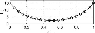
Figure 1: Profile of $\Gamma_{i}$ obtained from Eq.(4), when $\Gamma_{0}=15,\xi=5$.

II.3 Bistability

We assume that cells normally prefer to live in a stable state, and cells with a high concentration of active factor are capable of switching between two states. This kind of bistability is very important and has been observed in various biological systems Angeli et al. (2007). For example, the expression of the Dictyostelium cAMP phosphodiesterase gene behave as a bistable switch employing intracellular cAMP as a regulator of cell fate Riley and Barclay (1990), the Cdc2 activation system in Xenopus egg extracts is bistable and characterized by biochemical hysteresis Pomerening et al. (2003), the inducible lac operon in E. coli shows bistability Santillan et al. (2007), and so on.

Usually, bistability arises from positive, or double-negative genetic regulation loops Kim et al. (2008); Angeli et al. (2007); Holt et al. (2008). It was recently suggested that stochastic fluctuation plays an important role in the nature of the transition between bistable states Maamar et al. (2007); Losick and Desplan (2008). Moreover, physical regulation of protein production, which has been much less considered by biochemists, also plays an important role in the origin of the bistability. It has been observed that discrete transition between folding and unfolding states, namely a first-order phase transition, can take place in giant DNA Luckel et al. (2005). Similar discrete switch can also occur for RNA Mamasakhlisov et al. (2007), protein Schanda et al. (2007) and other molecules Etienne-Manneville and Hall (2002). This discrete transition leads to the ON/OFF switching of the production of a specific protein.

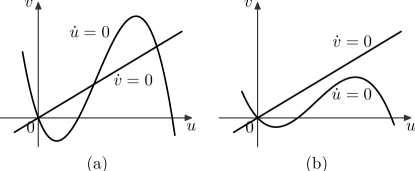
Figure 2: Nullcline diagrams in bistability (a) and mono-stability (b), respectively.

II.4 Model equations

We describe the dynamical reaction function of each cell by using the two-component Fitzhugh-Nagumo equations

$$\dot{u} =f(u,v,\Gamma)=\Gamma u(u-\alpha)(1-u)-v$$ (5)

$$\dot{v} =g(u,v)=\epsilon(\beta u-v)$$ (6)

where $u$ is a variable related to the expression level of specific activator genes, $v$ is the inhibitor to repress $u$, $\epsilon$, which is much smaller than 1, is the slower growth factor of inhibitor $v$ and $\Gamma$ is the active factor discussed previously. Note that the kinetics of inhibitor here is a rather natural unit process in many of biochemical reactions. Throughout this paper, the following parameters are fixed

$$\alpha=0.3,\ \beta=0.5,\ \epsilon=0.02.$$ (7)

The Fitzhugh-Nagumo model has been well studied for description of excitable behavior in biology. Rich nonlinear dynamics can be observed by tuning parameters. Specifically, with the above parameters, the model is mono-stable at small value of $\Gamma$, and will happen a saddle-node bifurcation at $\Gamma=4.08$ and a Hopf bifurcation at $\Gamma=4.27$, which leads to bistability. Thus, in the case of the spatial profile of $\Gamma_{i}$ as shown in Fig. 1, only the 8 central cells (7^th - 14^th) are mono-stable, while the others are bistable ($\Gamma_{6}=\Gamma_{15}=4.37$).

Figures 2(a)&(b) show the nullclines with bistability and mono-stability for when $\Gamma$ is large and small, respectively. Again, none of the cells show oscillation in the absence of coupling. More important, from the geometry property of nullclines in the figure, no oscillatory condition could be found by moving cubic nullcline ($\dot{u}=0$) up and down. That is, no pacemaker cells can be generated from activator coupling.

If we substitute Eq. (5&6) into Eq. (1&2), we get the system equations used in this paper.

$$\dot{u}_{i} =\Gamma_{i}u_{i}(u_{i}-\alpha)(1-u_{i})-v_{i}$$ (8)

$$\ \ \ +\tilde{D}(u_{i-1}+u_{i+1}-2u_{i})$$

$$\dot{v}_{i} =\epsilon(\beta u_{i}-v_{i})$$ (9)

When we change the coupling strength $\tilde{D}$, we observe the occurrence, variation and disappearance of self-sustained collective oscillation in the cell array.

III Self-sustained collective oscillation

III.1 Normal collective oscillation

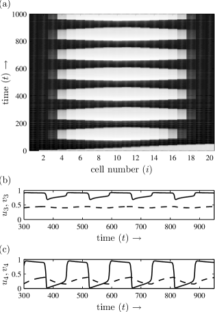
Figure 3: Collective oscillation observed in a chain of cells when $\tilde{D}=0.7$ in Eqs. (8& 9). (a) Spatio-temporal plot of the collective oscillation of $u_{i}$. The black and white indicate $u_{i}=1$ and $u_{i}=0$, respectively. (b, c) Waveforms of $u$ (solid) and $v$ (dashed) in the 3rd and 4th cells.

Figure 3(a) shows a typical oscillation when the coupling strength $\tilde{D}=0.7$. Figure 4(a) shows an enlarged view of a single period of oscillation. As the initial condition, we set the 1st cell as being excited, since stimulation is usually input from the border. Initially, ($0<t\lesssim 80$), a traveling wave appears due to excitation at the border. The traveling front then sweeps over the cell array and makes all of the cells excited (see Fig. 4(b)). Although the central cells are also turned ON due to the interaction with other cells, they can not stay in the excitable state for a long time. Instead, they soon return to their stable equilibrium (see Fig. 4(c)), and hence generate two counterpropagating wave backs, as shown in Fig. 4(d). These two wave backs propagate outward until the 3^rd and 18^th cells and stop suddenly due to the spatial discreteness (see Fig. 4(e)). The “wall” cells do not jump from the ON state to the OFF state and only exhibit slight oscillation closed to their equilibrium. As an example, the difference between the 3^rd and 4^th cells is shown in Fig. 3(b, c). At this critical interface, the inhibitor $v$ slowly decreases so that the 4^th and 17^th cells restore excitability after a while. The central cells can then be excited again by the pair of reflecting wave fronts, as shown in Fig. 4(f). Pushed by the wave, the central cells will be excited again. This process repeats and causes the collective oscillation inside multi-cell tissue without oscillatory cells.

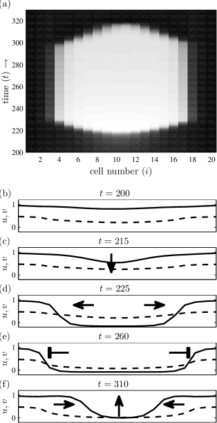
Figure 4: (a) Spatio-temporal diagram of $u_{i}$ over a single period, (b)-(f) Snapshots of $u$ and $v$ at several time points in one period, where the horizontal axis is cell number from 1 to 20. This illustrates the change in wave propagation at different stages. Solid curves and dashed curves indicate $u$ and $v$, respectively. An animation, through which the behavior can be understood more intuitively, is available at URL (url).

III.2 Stationary state before birth of oscillation

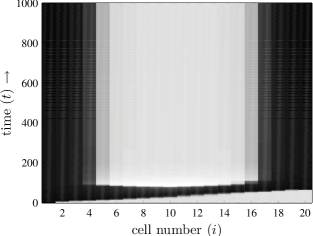
Figure 5: Spatio-temporal diagram of $u_{i}$ in a stationary state. Wave propagation stops and no oscillation occurs in the case of weak coupling $\tilde{D}=0.47$.

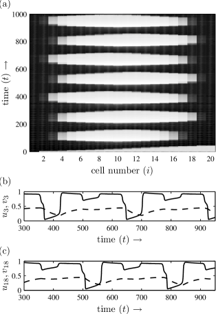
Figure 6: Anti-phase mode in period doubling produces collective oscillation with a periodic position shift when $\tilde{D}=0.8$. (a) Spatio-temporal diagram of $u_{i}$. The grayscale black and white indicate $u_{i}=1$ and $u_{i}=0$, respectively. (b) and (c) are waveform diagrams of the 3rd and 18th cells. Activator $u$ and inhibitor $v$ are shown in solid and dashed curves, respectively.

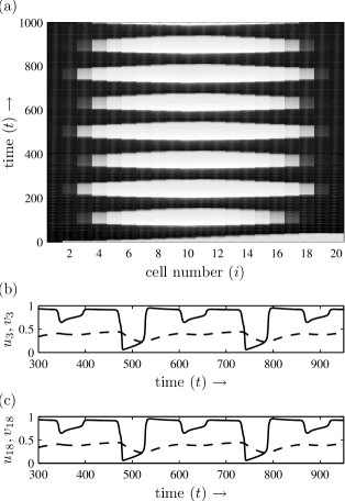
Figure 7: In-phase mode in period doubling produces collective oscillation with a change in the periodic population when $\tilde{D}=0.9$. (a) Spatio-temporal diagram of $u_{i}$. The grayscale black and white indicate $u_{i}=1$ and $u_{i}=0$, respectively. (b) and (c) are waveform diagrams of the 3^rd and 18^th cells. Activator $u$ and inhibitor $v$ are shown in solid and dashed curves, respectively.

The above collective oscillation can be observed when the coupling strength is larger than a threshold, below which wave backs (see Fig. 4(d)) fail to reflect, and the state in Fig. 4(e) is maintained. Figure 5 shows a spatio-temporal diagram, where the central cells stay silent while excited bands appear close to the two borders.

Note that this phenomenon could not take place in a continuum counterpart. The existence of a coupling strength threshold under which wave propagation failure occurs is unique to a spatially discrete system. In addition, there is another threshold, which is even smaller, for which the wave front stops propagating. In this case, the excited signal at the border fails to propagate forward, but we would like to postpone this interesting phenomenon on another paper, since it is less related to present work.

III.3 In-phase and anti-phase period doubling oscillation closed to the boundary

With an increase in the coupling strength $\tilde{D}$, the characteristics of oscillation can be changed. Figure 6 shows that the position of oscillation periodically shifts. The 3^rd and 18^th cells oscillate with a nearly doubled period, in anti-phase (Fig. 6(b,c)). Globally, tissue oscillates in two groups with the same cell populations but different positions: No. 3-No. 17 (15 cells) and No. 4-No. 18 (15 cells), respectively.

Interestingly, by slightly increasing the coupling strength $\tilde{D}$, say to $\tilde{D}=0.9$, we found a different type of period doubling, as shown in Fig. 7. For comparison with the case of $\tilde{D}=0.8$, although the critical interface between ON and OFF shifts periodically as in Fig. 6, there is no phase difference between the 3^rd and 18^th cells. As is clearly shown in their waveform (Fig. 7(b,c)), these two boundary cells oscillate in-phase, instead of anti-phase (Fig. 6(b,c)). Therefore, in the present condition, a periodic change does not take place in the position of oscillation. Instead, the population of oscillating cells changes. More precisely, tissue oscillates in two groups: No. 3-No. 18 (16 cells) and No. 4-No. 17 (14 cells), respectively.

Moreover, by setting the initial condition of the cells identically, i.e., all in the ON state at $t=0$, we found checked that same symmetric collective oscillation can also occur in the case of $\tilde{D}=0.8$. Therefore, we conclude that these two types of oscillation are caused by the same bifurcation. Because the wavefront propagates faster with larger $\tilde{D}$, a larger coupling strength can reduce the time lag between the two boundary cells being stimulated. If the time lag is smaller, the two boundaries converge to in-phase oscillation. On the other hand, if the time lag is large, they will exhibit anti-phase oscillation.

III.4 Oscillation death

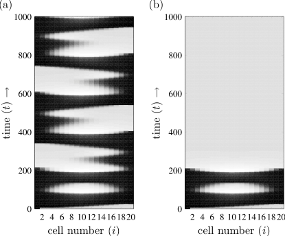
Figure 8: Spatio-temporal diagram of $u_{i}$. Black and white indicate $u_{i}=1$ and $u_{i}=0$, respectively. (a) $\tilde{D}=2.53$, oscillation starts to collapse; (b) $\tilde{D}=2.6$, oscillation ceases after one cycle.

With a increase in coupling strength $\tilde{D}$, we observed that the change in the periodic position or population stopped, and normal oscillation returned. In comparison to the case of $\tilde{D}=0.7$, the total population of oscillating cells increased from 14 (No. 4 to No. 17) to 16 (No. 3 to No. 18).

The oscillation suddenly dies when $\tilde{D}$ is as large as 2.6. Figure 8(b) clearly shows that the central cells start to oscillate after all of the cells are excited, but this oscillation is not sustained. In this strong coupling condition, the boundary cells can not recover their excitability, so that the wave front propagating from the center is unable to stop and reflect to generate successive oscillation.

Before the oscillation stops, there is a narrow parameter region of $2.53\leqslant\tilde{D}\leqslant 2.56$, where only one side of the “wall” alternatively collapses, and a complicated period-4 collective oscillation is observed (Fig. 8(a)).

III.5 Overall perspective and bifurcation

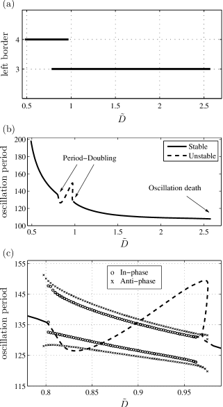
Figure 9: Phase diagram of (a) cell number for the left boundary of collective oscillation. (b) the oscillation period, (c) an enlarged view with in-phase and anti-phase period two solutions, with respect to the change in the strength of coupling.

There are many factors that may influence the oscillation behavior. For example, if the spatial profile of active factor $\Gamma$ becomes more “steep” rather than a gentle slope, the wave back will tend to be locked and fail to reflect from boundary. Moreover, if we reduce the excitability of cells by increasing $\epsilon$, it will be more difficult for wave front to propagate cross the center, and only the half part with stimulation can oscillate. Since the global oscillation is induced by mutual coupling, we are going to study the oscillation behavior with respect to the coupling strength. Here, we sweep $\tilde{D}$ from 0.45 to 2.7, and summarize the variation in the oscillation period and position of the left border of oscillation region.

If the coupling strength is smaller than 0.48, there is no oscillation, and 4 cells from the tissue border are excited while cells 5–16 are silent. Oscillation takes place when the wave back passes the 4^th cell at $\tilde{D}=0.48$. The border then shifts between 3 and 4, while in-phase and anti-phase period doubled oscillation occur, roughly between $0.78<\tilde{D}<0.97$. Finally, the oscillation reaches a maximum region: from cells 3 to 18, until $\tilde{D}$ is too large for oscillation to occur. Figure 9(a) shows the expansion of oscillatory region.

Variations in the period of oscillation are shown in Fig. 9(b). Once the central cells start to collectively oscillate, The period rapidly decreases when the coupling strength increases. The rate of the period decrease gradually slows. The period changes little in the region where $\tilde{D}$ is large. This phenomenon occurs because the stationary interval (Fig. 4(e)) greatly contributes to the period of oscillation. The decrease in the stationary interval significantly shortens the period of oscillation when $\tilde{D}$ is small. However, when $\tilde{D}$ is large enough, the wave backs reflect immediately without stopping, and the period is determined mainly by the velocity of propagation. Therefore, the presented oscillation is robust at strong coupling condition, and tunable at weak coupling case.

There is a parameter region (the curve of period is drawn in dashed curve Fig. 9(b)) in which system undergoes Period-Doubling bifurcation and the period-1 solution lose its stability. Meanwhile, period two solutions appear around this region. We show more details in Fig. 9(c). In the figure, we draw two intervals in a period two solution, by measuring the time when $u_{4}$ positively cross the section: $u_{4}=0.5$. Circles ($\circ$) and crosses ($\times$) indicate in-phase and anti-phase solutions, respectively. The in-phase period-2 solution is the result of Period-Doubing bifurcation, while the anti-phase period-2 solution occurs saddle-node bifurcation. The anti-phase period-2 solution has a wider parameter region than in-phase one, and coexistence with fundamental period-1 solution can be observed in both side of $\tilde{D}$. There are quite complicated bifurcation phenomena specially around the occurrence of Period-Doubling bifurcation. We have even found period-3 solution (in-phase one around $\tilde{D}$=0.802, and anti-phase one around $\tilde{D}=0.975$, respectively). Although they are very interesting in the viewpoint of nonlinear dynamical system, we leave them to our future work, because current paper is going to discuss the possibility of global oscillation and its potential applications.

IV Discussion

IV.1 Discreteness vs. continuum

The above phenomena are observed in a spatially discrete system, described by ordinary differential equations. As briefly introduced in Sec I, this discreteness is important in both a mathematical and biological sense. Let us discuss this significance in more detail.

The diffusion term $D(\partial^{2}u/\partial x^{2})$ in a one-dimensional spatially continuous reaction-diffusion model can be formulated as $D(u_{i-1}+u_{i+1}-2u_{i})/\Delta x^{2}$ in its difference version. This type of conversion is a common approach to solving PDE numerically. The diffusion rate $D$ usually does not change much for a specific substance under constant conditions. Thus, if we assume that the coupling is mainly due to the diffusion-like effects of substances, the coupling strength $\tilde{D}\approx D/\Delta x^{2}$ changes in square order with respect to variation of $\Delta x$, which biologically corresponds to the distance between cells or the cell size. Since the profile of the active factor has a scaling property, it is reasonable to suppose that this gradient works for a field of any size. Thus, we can study how a change in number of cells $N$ and distant of cells $\Delta x$ affects global dynamics.

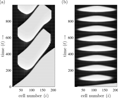
Figure 10: Spatio-temporal diagram of $u_{i}$. Black and white indicate $u_{i}=1$ and $u_{i}=0$, respectively. $N=200$. (a) $\tilde{D}=D/\Delta x^{2}=0.7$. (b) $\tilde{D}=D/\Delta x^{2}=70$.

Figure 10(a) shows spatio-temporal diagrams with a 10-fold increase in the number of cells, $N=200$. Other parameters are the same as those in Fig. 3. Obviously, more time is required for a wave to sweep over the organism. The period of oscillation and the phase difference between the two sides increase greatly. On the other hand, if the distance $\Delta x$ between cells becomes smaller and smaller when cell population increases, the system manifests itself more like a continuum than a discrete system. In this case, the coupling strength will increase dramatically as a square with respect to the decrease in $\Delta x$, i.e., a 100-fold increase in $\tilde{D}$ in present case. When $\tilde{D}$ is as large as 70, we have the spatio-temporal diagram given in Fig. 10(b). When we compare this with Fig. 3, there is little change in the period of collective oscillation. This suggests that the clock tends to run more punctually. In a mathematical sense, when the population of cells is large enough in a fixed field, the behavior of the organism will follow the solution of a specific partial differential equation, which is independent of the number of cells.

Figure. 10(a) simply corresponds to the case that cells grow in an open space, and extend the field by keeping size and distant of cells constantly. During the initial period of development, however, cell divisions within the egg proceed quickly, without much increase of the total cell mass and size. Thus, cells at this stage rapidly decrease in diameter. This may interpret biologically the situation of Fig. 10(b).

There are many biological situations, however, that the intercellular coupling does not follow the diffusion-like ways, such as communication involving the delta-notch signaling pathway Mumm and Kopan (2000). In those cases, $\Delta x$ has few direct influences on $\tilde{D}$, which may represent “bottlenecks” irrespective to the diffusion. Thus, the modeling based a continuum is inappropriate for some conditions.

IV.2 Understanding the mechanism

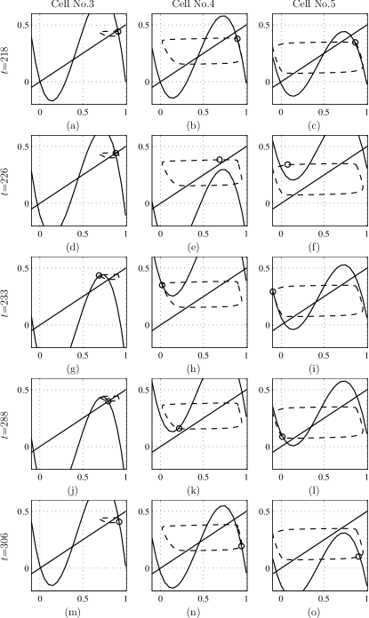
Figure 11: Phase portrait diagrams with snapshots of the dynamical nullcline. Rows indicate the time evolution from the top down, and columns indicate the number of cells (3 at left, 4 at middle and 5 at right). Dashed curves are the limit cycle solution. Cubic function curves are the nullcline of $\dot{u}_{i}=0$. Straight lines are the nullcline of $\dot{v}_{i}=0$. Circles are the position of $(u_{i},v_{i})$ at specific times. An animation of the dynamical nullclines can be found at URL (url).

Self-sustained collective oscillation is caused by the excitability of cells and their mutual interaction. The system involves complicated bifurcations. We present here some qualitative ideas regarding how this oscillation takes place.

From dynamical equations (5,6) and their nullcline shown in Fig. 2, we know that a single cell can exhibit either bistability or mono-stability. However, if we introduce coupling, the geometry of nullclines of one cell will dynamically change according to its own state and those of its neighbors. Because it was assumed that the communication between cells is only mediated via the activator $u$, the strict nullcline $\dot{v}_{i}=0$ is independent of coupling.

$$v_{i}=G(u_{i})=\beta u_{i}.$$ (10)

From Eqs.(1&5), we obtain the function for the nullcline $\dot{u}_{i}=0$ as

$$v_{i}=F(u_{i},\Gamma_{i})=\Gamma_{i}u_{i}(u_{i}-\alpha)(1-u_{i})+\Delta U_{i},$$ (11)

where $\Delta U_{i}=\tilde{D}(u_{i+1}+u_{i-1}-2u_{i})$ is the offset of the cubic function due to coupling. Thus, the nullcline $v=F(\cdot)$ dynamically moves up and down in the phase plane, corresponding to the state of $u_{i-1},u_{i},u_{i+1}$.

In Fig. 11, we show the phase portrait of cells around the oscillation border (cells No.3-5), as well as their dynamical nullcline at some turning points. Snapshots are taken under the same conditions of normal oscillation as shown in Fig. 3.

The first row, (a, b, c) of Fig. 11 are all in the excited state, i.e., for all three cells, $u_{i}$ is close to 1. Therefore, under this condition, the vertical offset $\Delta U$ of the nullcline is nearly zero, and all three cells exhibit bistability. The second row is taken at $t=226$, when the wave back comes (see Fig. 4(d)), and the 5^th cell moves towards its lower equilibrium (Fig. 11(f)). Since $\Delta U_{4}=\tilde{D}(u_{3}+u_{5}-2u_{4})$, a sudden drop in $u_{5}$ leads to a rapid decrease in the cubic nullcline. As shown in Fig. 11(e), the cubic nullcline moves down so that the higher equilibrium disappears. Thus, the 4^th cell becomes mono-stable and the state quickly converges to the left branch of the cubic nullcline. The decrease in $u_{4}$ pushes $\Delta U_{4}$ back to a positive value, and makes the nullcline of the 3^rd cell move down, as shown in Fig. 11(g, h). However, since the 3^rd cell has a larger $\Gamma$, which controls the amplitude of the cubic nullcline, even if $u_{4}$ decreases to its lowest value (Fig. 11(h)), i.e., $\Delta U_{3}$ reduces to its minimum, the cubic and straight nullclines still intersect, and the higher equilibrium remain. This explains why the wave back passes the 4^th cell, but stops at the 3^rd cell (Fig. 4(a)). After propagation stops, there is a relatively long refractory period from time 230 to 300. In this interval, there is a slow decrease in the inhibitor $v_{4}$. Since $u_{3}\approx 0.8$ and $u_{5}\approx 0$, although slight increase in $u_{4}$ pulls the cubic nullcline down, $\Delta U_{4}$ is still so large that the cubic nullcline is above the straight nullcline (Fig. 11(k)). Under this condition, the cell is mono-stable, with the equilibrium at the right branch of the cubic function. Thus, after a while, the state of $u$ will switch to a higher value (Fig. 11(n)), and leads to a reflecting wave front (Fig. 4(f)). Finally, the states return to the situation of Fig. 11(b) after another refractory period.

Note that a smaller coupling strength $\tilde{D}$ leads to a smaller offset $\Delta U$. If we move down the cubic nullcline slightly to cross the straight nullcline in Fig. 11(k), the 4^th cell becomes bistable. This will disable the switch from left to right, and stop the oscillation (Fig. 5).

From the above description and Fig. 11, we conclude that the boundary cell, here No.4, which is bistable without coupling, turns to switch between two types of mono-stable dynamics. As introduced in Sec. I, it is different from the studies changing nullclines via coupling to an oscillatory geometry. This switching becomes the power that underlies the self-sustained oscillation observed in the present model. The variation of the offset of the dynamical nullcline of the boundary cell gives rise to rich oscillation phenomena.

IV.3 Conditions for oscillation

We will now explore the conditions for oscillation in an approximate manner by studying the dynamics on the oscillation border, where wave backs (WB) stop and wave fronts (WF) generate. Based on an investigation of the dynamical nullcline and state variable, we concluded that a wave back will not pass a critical cell, $c$, if the nullclines still intersect at the right branch when cell $c+1$ has dropped to its lower equilibrium (Fig. 11(g,h)). In contrast, if the intersections disappear, the state of $u_{c}$ will switch to a lower equilibrium. Then cell $c$ is possible to oscillate, if it fires a wave front, in the case that the two nullclines do not cross at the left branch when the state of the inhibitor recovers to its lower limit (Fig. 11(e,f)).

Thus, we can roughly solve the condition by finding two possible tangency for the two nullclines Eq. (10) and Eq. (11). This can be achieved using the following equations:

$$\frac{{\rm d}F(u,\Gamma)}{{\rm d}u}=\frac{{\rm d}G(u)}{{\rm d}u},$$ (12)

Equation (12) is for two nullclines with the same slope. By substituting $F$ and $G$ into Eq. (12), we have

$$\Gamma(-3u^{2}+2(1+\alpha)u-\alpha)=\beta,$$ (13)

from which we obtain two solutions

$$u_{T_{1,2}}=\frac{13\pm\sqrt{79-150/\Gamma}}{30}.$$ (14)

For cell $c$ to propagate a wave back, there should be only a lower equilibrium when $u_{c}$ close to the higher tangency point. The corresponding condition is $F(u_{T_{1}},\Gamma_{c})<G(u_{T_{1}})$. Substitution leads to

$$\Gamma_{c}u_{T_{1}}(u_{T_{1}}-\alpha)(1-u_{T_{1}})+\tilde{D}(u_{c-1}+u_{c+1}-2u_{T_{1}})<\beta u_{T_{1}}.$$ (15)

On the other hand, for cell $c$ to generate a wave front, there should be no lower equilibrium when $u_{c}$ is close to the lower tangency point. This simply means that $F(u_{T_{2}},\Gamma_{c})>G(u_{T_{2}})$, which can be rewritten as

$$\Gamma_{c}u_{T_{2}}(u_{T_{2}}-\alpha)(1-u_{T_{2}})+\tilde{D}(u_{c-1}+u_{c+1}-2u_{T_{2}})>\beta u_{T_{2}}.$$ (16)

Two critical conditions are shown in Fig. 12.

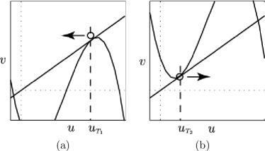
Figure 12: Schematic diagram of two critical tangency situations, corresponding to the conditions for which (a) a wave back passes and (b) a wave front is generated. Black circles are the position of states when two nullclines tangent to each other.

Approximation

1. $u_{c-1}$ is the “distal” side of the critical cell $c$. It remains in its higher equilibrium since the wave back can not pass it. Thus, we can approximate it by finding the biggest intersection of the two nullclines. In the wave back case, since $u_{T_{1}}$ is close to the higher equilibrium, $\Delta U_{c-1}$ is nearly zero. Thus, we determine $u_{c-1}$ to be 0.9. In the wave front case, however, $u_{T_{2}}$ is small. If we consider the minus $\Delta U_{c-1}$, we determine $u_{c-1}$ to be 0.8.

2. $u_{c+1}$ is the “proximal” side of the critical cell $c$. It switches off before cell $c$ when a wave back comes and waits to be excited again by cell $c$, so at the critical time, $u_{c+1}$ approaches 0.

3. Figure 13 shows $u_{T_{1,2}}$ according to Eq. (14). Obviously, $u_{T_{1}}$ and $u_{T_{2}}$ change little, and can be regarded as the constants $0.7$ and $0.17$, respectively.

4. Note that the above approximations are not valid when the coupling strength is too large, or excitability is too weak.

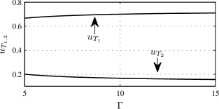
Figure 13: Variation of two tangent points $u_{T_{1,2}}$ with respect to $\Gamma$.

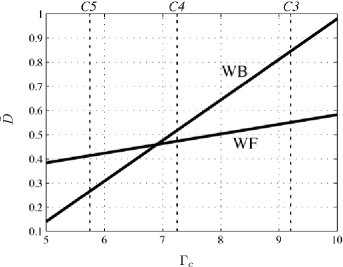
Figure 14: The diagram in the parameter plan ($\Gamma_{c},\tilde{D}$) representing the conditions of collective oscillation. A wave back passes the cell, and a wave front reflects, when the parameters are above the WB and WF line, respectively.

According to the above approximations, by substituting

$$u_{T_{1}}=0.7,u_{c-1}=0.9,u_{c+1}=0$$

into Eq. (15), and

$$u_{T_{2}}=0.17,u_{c-1}=0.8,u_{c+1}=0$$

into Eq. (16), we obtain two rough conditions

$$\tilde{D}>0.168\Gamma_{c}-0.7$$ WB passes, (17)

$$\tilde{D}>0.0398\Gamma_{c}+0.1848$$ WF generates. (18)

Clearly, the critical coupling strength increases linearly with respect to the active factor $\Gamma$. We draw two lines in Fig. 14, where the WB and WF lines are obtained from Eq. (17) and Eq. (18), respectively.

In Fig. 14, labels C3, C4 and C5 on the top horizontal axis indicate the value of $\Gamma$ defined by Eq. (4) for cells 3, 4 and 5, respectively. Lines WF and WB cross each other between C4 and C5. This kind of topology makes the 4^th and 5^th cells behave completely different.

For cell 5, WF is above WB. If the coupling strength is between WF and WB, a wave back coming from the center can switch the 4^th cell OFF, but the cell can not be switched ON to fire a wave front. This is exactly the situation shown in Fig. 5, in which no oscillation takes place. On the other hand, for cell 4, WF is below WB. Clearly, if the coupling strength allows the wave back to suppress the 4^th cell, the cell will be excited again and lead to a wave front.

The conditions for these two situations depend on many other factors, such as the initial conditions, propagation velocity, cell excitability, and so on. The situation is much more complicated than the approximated case we have discussed here. Qualitatively, we can conclude that the intersection of these two condition lines is the origin of self-sustained collective oscillation.

V Concluding remarks

In this paper, we have proposed a scenario for self-organized and self-sustained oscillation in multi-cellular biological tissue. In contrast to the usual framework based on an oscillatory genetic network, the present system does not include any self-oscillating cells. However, by mutual coupling, we can observe collective oscillation inside a group of cells, i.e., tissue. Moreover, oscillation can manifests itself in several ways, corresponding to different coupling strengths. Anti-phase and in-phase oscillations at the two boundaries lead to changes in the position of oscillation and the oscillating cell population, respectively. The birth and death of oscillation resulting from variation in the coupling strength were also discussed. We also provide a general idea of how the size of the cell and population affects the oscillatory behavior. Finally, a detailed investigation of the dynamical movement of the nullcline provided insight into the mechanism of complicated oscillatory phenomena. Although there have been several studies on self-oscillatory phenomena in spatially discrete systems in the context of mathematics and physics, this paper extends these basic ideas to spatio-temporal self-organization in a biological system. It is of interest to extent our new hypothesis to spatial three dimensional systems, i.e., a more realistic model of living organism.

Our observations were based on a numerical simulation. Future analytical studies inspired by these interesting phenomenon are needed. At last, but not less important, we are going to cooperate with biologists, in order to design corresponding biological experiments and to explore more proofs supporting our hypothesis.

References

- Schibler and Naef (2005) U. Schibler and F. Naef, Current Opinion in Cell Biology 17, 223 (2005).
- Pourquie (2003) O. Pourquie, Science 301, 328 (2003).
- Stark et al. (2007) J. Stark, C. Chan, and A. J. T. George, Immunological Reviews 216, 213 (2007).
- Tiana et al. (2007) G. Tiana, S. Krishna, S. Pigolotti, M. H. Jensen, and K. Sneppen, Physical Biology 4, R1 (2007).
- Hirata et al. (2002) H. Hirata, S. Yoshiura, T. Ohtsuka, Y. Bessho, T. Harada, K. Yoshikawa, and R. Kageyama, Science 298, 840 (2002).
- Hoffmann et al. (2002) A. Hoffmann, A. Levchenko, M. L. Scott, and D. Baltimore, Science 298, 1241 (2002).
- Lewis (2003) J. Lewis, Current Biology 13, 1398 (2003).
- Chen and Aihara (2002) L. Chen and K. Aihara, Circuits and Systems I, IEEE Transactions on 49, 1429 (2002).
- Masamizu et al. (2006) Y. Masamizu, T. Ohtsuka, Y. Takashima, H. Nagahara, Y. Takenaka, K. Yoshikawa, H. Okamura, and R. Kageyama, PNAS 103, 1313 (2006).
- Gonze and Goldbeter (2006) D. Gonze and A. Goldbeter, Chaos 16, 026110 (2006).
- Garcia-Ojalvo et al. (2004) J. Garcia-Ojalvo, M. Elowitz, and S. Strogatz, PNAS 101, 10955 (2004).
- Pérez-Armendariz et al. (1991) M. Pérez-Armendariz, C. Roy, D. C. Spray, and M. V. Bennett, Biophysical Journal 59, 76 (1991).
- Bertram and Sherman (2000) R. Bertram and A. Sherman, J Biosci 25, 197 (2000).
- Rust et al. (2007) M. J. Rust, J. S. Markson, W. S. Lane, D. S. Fisher, and E. K. O’Shea, Science 318, 809 (2007).
- Mehra et al. (2006) A. Mehra, C. I. Hong, M. Shi, J. J. Loros, J. C. Dunlap, and P. Ruoff, PLoS Computational Biology 2, e96 (2006).
- O’Neill et al. (2008) J. S. O’Neill, E. S. Maywood, J. E. Chesham, J. S. Takahashi, and M. H. Hastings, Science 320, 949 (2008).
- Smale (1974) S. Smale, in The Hopf Bifurcation and Its Application, edited by J. E. Marsden and M. McCracken (Springer-Verlag, NY, 1974), chap. 11.
- Pogromsky (1998) A. Y. Pogromsky, International Journal of Bifurcation and Chaos 8, 295 (1998).
- Pogromsky et al. (1999) A. Pogromsky, T. Glad, and H. Nijmeijer, International Journal of Bifurcation and Chaos pp. 629–644 (1999).
- Gomez-Marin et al. (2007) A. Gomez-Marin, J. Garcia-Ojalvo, and J. M. Sancho, Physical Review Letters 98, 168303 (2007).
- In et al. (2003) V. In, A. R. Bulsara, A. Palacios, P. Longhini, A. Kho, and J. D. Neff, Physical Review E 68, 4 (2003).
- Yanagita et al. (2005) T. Yanagita, Y. Nishiura, and R. Kobayashi, Physical Review E 71, 036226 (2005).
- Nekhamkina and Sheintuch (2006) O. Nekhamkina and M. Sheintuch, Physical Review E 73, 066224 (2006).
- Cartwright (2000) J. H. Cartwright, Physical review E 62, 1149 (2000).
- Lewis and Rinzel (2000) T. Lewis and J. Rinzel, Network: Computation in Neural Systems 11, 299 (2000).
- Coullet et al. (1990) P. Coullet, J. Lega, B. Houchmanzadeh, and J. Lajzerowicz, Physical Review Letters 65, 1352 (1990).
- Hagberg and Meron (1994) A. Hagberg and E. Meron, Chaos 4, 477 (1994).
- Bode (1997) M. Bode, Physica D: Nonlinear Phenomena pp. 270–286 (1997).
- Prat and Li (2003) A. Prat and Y. Li, Physica D: Nonlinear Phenomena pp. 50–68 (2003).
- Prat et al. (2005) A. Prat, Y. Li, and P. Bressloff, Physica D: Nonlinear Phenomena pp. 177–199 (2005).
- Li (2003) Y. Li, Physica D: Nonlinear Phenomena pp. 27–49 (2003).
- Miyazaki and Kinoshita (2007) J. Miyazaki and S. Kinoshita, Physical Review E 76, 066201 (2007).
- Shnerb et al. (2000) N. M. Shnerb, Y. Louzoun, E. Bettelheim, and S. Solomon, PNAS 97, 10322 (2000).
- Keener (1987) J. P. Keener, SIAM J. Appl. Math. 47, 556 (1987).
- Turing (1952) A. M. Turing, Philos. Trans. R. Soc. London B327, 37 (1952).
- Kageyama et al. (2007) R. Kageyama, Y. Masamizu, and Y. Niwa, Developmental Dynamics 236, 1403 (2007).
- Ibanes and Belmonte (2008) M. Ibanes and J. C. I. Belmonte, Molecular Systems Biology 4 (2008).
- Ben-Zvi et al. (2008) D. Ben-Zvi, B.-Z. Shilo, A. Fainsod, and N. Barkai, Nature 453, 1205 (2008).
- Wolpert (1969) L. Wolpert, J. Theoret. Biol. 25, 1 (1969).
- Lewis (2008) J. Lewis, Science 322, 399 (2008).
- Angeli et al. (2007) D. Angeli, J. James E. Ferrell, and E. D. Sontag, PNAS 101, 1822 (2007).
- Riley and Barclay (1990) B. B. Riley and S. L. Barclay, Proceedings of the National Academy of Sciences of the United States of America 87, 4746 (1990).
- Pomerening et al. (2003) J. R. Pomerening, E. D. Sontag, and J. E. Ferrell, Nat Cell Biol 5, 346 (2003).
- Santillan et al. (2007) M. Santillan, M. Mackey, and E. Zeron, Biophysical Journal 92, 3830 (2007).
- Kim et al. (2008) J.-R. Kim, Y. Yoon, and K.-H. Cho, Biophysical Journal 94, 359 (2008).
- Holt et al. (2008) L. J. Holt, A. N. Krutchinsky, and D. O. Morgan, Nature 454, 353 (2008).
- Maamar et al. (2007) H. Maamar, A. Raj, and D. Dubnau, Science 317, 526 (2007).
- Losick and Desplan (2008) R. Losick and C. Desplan, Science 320, 65 (2008).
- Luckel et al. (2005) F. Luckel, K. Kubo, K. Tsumoto, and K. Yoshikawa, FEBS Letters 579, 5119 (2005).
- Mamasakhlisov et al. (2007) Y. S. Mamasakhlisov, S. Hayryan, V. F. Morozov, and C.-K. Hu, Physical Review E 75, 061907 (2007).
- Schanda et al. (2007) P. Schanda, V. Forge, and B. Brutscher, PNAS 104, 11257 (2007).
- Etienne-Manneville and Hall (2002) S. Etienne-Manneville and A. Hall, Nature 420, 629 (2002).
- Mumm and Kopan (2000) J. S. Mumm and R. Kopan, Developmental Biology 228, 151 (2000), ISSN 0012-1606.
- URL (url) Movies and some more details are available at URL: http://ma-yue.net/study/selfosc/