Quantum Oscillations Can Prevent the Big Bang Singularity in an Einstein-Dirac Cosmology

Abstract.

We consider a spatially homogeneous and isotropic system of Dirac particles coupled to classical gravity. The dust and radiation dominated closed Friedmann-Robertson-Walker space-times are recovered as limiting cases. We find a mechanism where quantum oscillations of the Dirac wave functions can prevent the formation of the big bang or big crunch singularity. Thus before the big crunch, the collapse of the universe is stopped by quantum effects and reversed to an expansion, so that the universe opens up entering a new era of classical behavior.

Numerical examples of such space-times are given, and the dependence on various parameters is discussed. Generically, one has a collapse after a finite number of cycles. By fine-tuning the parameters we construct an example of a space-time which is time-periodic, thus running through an infinite number of contraction and expansion cycles.

1. Introduction, the Einstein-Dirac System

Near the big bang or big crunch singularity, the matter density and the space-time curvature become arbitrarily large. It is generally believed that in this regime, quantum effects should come into play, which could even prevent the formation of the singularity. This effect has first been analzyed in [7] for classical gravity coupled to a second quantized matter field; see also [9]. For a quantized gravitational field, this effect has been studied in [6], and it was worked out in more detail in the framework of string cosmology [10] and in loop quantum gravity [1]. In contrast to the above approaches, we are here more modest and work with classical gravity coupled to Dirac wave functions, without using second-quantized fields. We find a new mechanism, based on the oscillations of the spin of the matter field, which tends to prevent the formation of a space-time singularity. The mechanism can be understood as a spin condensation effect. An advantage of our model is that it is very simple and can be analyzed without any approximations. The Dirac field could be interpreted physically as a new fermionic particle which becomes significant on the cosmological scale. Alternatively, the Dirac field can be understood similar to a “quintessence” [11] as effectively describing unknown fields acting in our universe on the large. Describing such a cosmological field by the Dirac equation seems physically natural and changes the behavior of the cosmological model drastically near the big bang or big crunch, where quantum oscillations can prevent the formation of space- time singularities depending on the initial conditions. Such a bounce back may happen several times, before, generically, the solution collapses. For brevity we here restrict attention to the case of a closed universe. However, the flat and hyperbolic cases are less interesting, since they expand infinitely. We remark that the hyperbolic case allows for solutions with negative energy density where the matter turns to be repulsive (see [4]).

For the derivation of the equations we follow the standard approach in [8, 3] where we work with a torsion free connection (for the effect of torsion see the cosmological model in Einstein-Cartan theory [2]). The Einstein-Dirac (ED) equations read

$$R^{i}_{j}-\frac{1}{2}R\>\delta^{i}_{j}=8\pi\kappa\,T^{i}_{j}\>,\qquad(\mathcal{D}-m)\Psi=0\>,$$ (1)

where $T^{i}_{j}$ is the energy-momentum tensor of the Dirac particles, $\kappa$ is the gravitational constant, $\mathcal{D}$ denotes the Dirac operator, and $\Psi$ is the Dirac wave function (we always work in natural units $\hbar=c=1$). For the metric we take the ansatz of the closed Friedmann-Robertson-Walker (FRW) geometry

$$ds^{2}=dt^{2}-R^{2}(t)\,d\sigma^{2},$$

where $t$ is the time for an observer at rest, $R$ is the scale function, and $d\sigma$ is the line element on the unit $3$-sphere,

$$d\sigma^{2}=\frac{dr^{2}}{1-r^{2}}+r^{2}d\vartheta^{2}+r^{2}\sin^{2}\vartheta\,d\varphi^{2}\>,$$

where $r\in(-1,1)$ is a radial variable, and $(\vartheta,\varphi)\in(0,\frac{\pi}{2})\times[0,2\pi)$ are the angular variables. The Dirac operator in this metric can be written as (see [3])

$$\mathcal{D}=i\gamma^{0}\left(\partial_{t}+\frac{3\dot{R}(t)}{2R(t)}\right)+\frac{1}{R(t)}\left(\begin{matrix}0&\mathcal{D}_{S^{3}}\\ -\mathcal{D}_{S^{3}}&0\\ \end{matrix}\right),$$ (2)

where $\gamma^{0}=\left(\begin{smallmatrix}\mbox{\rm{\scriptsize{1 1}}}&0\\ 0&-\mbox{\rm{\scriptsize{1 1}}}\\ \end{smallmatrix}\right)$ is the usual $4\times 4$ Dirac matrix, and $\mathcal{D}_{S^{3}}$ is the Dirac operator on the unit $3$-sphere. The operator $\mathcal{D}_{S^{3}}$ has discrete eigenvalues $\lambda=\pm\frac{3}{2},\pm\frac{5}{2},\ldots$, corresponding to a quantization of the possible momenta of the Dirac particles. For a given eigenvector $\psi_{\lambda}$, we can separate the Dirac equation with the ansatz

$$\Psi_{\lambda}=R(t)^{-\frac{3}{2}}\left[\frac{8\pi\kappa}{3}\left(\lambda^{2}-\frac{1}{4}\right)\right]^{-\frac{1}{2}}\left(\begin{matrix}\alpha(t)\>\psi_{\lambda}(r,\vartheta,\varphi)\\ \beta(t)\>\psi_{\lambda}(r,\vartheta,\varphi)\end{matrix}\right),$$ (3)

thus describing the time dependence of the wave function by two complex functions $\alpha$ and $\beta$. In order to be consistent with the homogeneous and isotropic ansatz of the metric, the Dirac spinors must also be in a homogeneous and isotropic configuration. In analogy to the method employed in [5] for spherical symmetry, this can be achieved by taking an anti-symmetrized product of the wave functions (3), where $\psi_{\lambda}$ runs over an orthonormal basis of the eigenspace corresponding to a fixed $\lambda$, where the symmetry is expressed by the fact that $\sum|\psi_{\lambda}(r,\vartheta,\phi)|^{2}=\lambda^{2}-\frac{1}{4}$, with the sum running over all corresponding angular quantum numbers. We thus obtain a fermionic Hartree-Fock state composed of $\lambda^{2}-\frac{1}{4}$ particles. The energy-momentum tensor $T^{i}_{j}$ can be derived in a similar way as in [5], see Equ. (4.4). By spherical symmetry the components $T^{t}_{r},T^{t}_{\vartheta},T^{t}_{\phi}$ have to vanish as well as the components $T^{r}_{\phi},T^{r}_{\vartheta},T^{\vartheta}_{\phi}$, which is due to the homogeneity in space. Therefore $T^{i}_{j}$ is a diagonal matrix where the space components are equal, again due to the fact that our system is homogeneous in space. Analogously to [5] we derive the time component of the energy-momentum tensor, which reads

$$T^{t}_{t}=\sum{\rm Tr}_{\mathbb{C}^{4}}\bigg{\{}i\gamma^{0}\left(\partial_{t}+\frac{3\dot{R}(t)}{2R(t)}\right)|\Psi_{\lambda}\rangle\langle\Psi_{\lambda}|\bigg{\}},$$

where the sum runs over the angular momentum quantum numbers, whose indices are suppressed for notational reason. Using (3) and the fact that the sum of $|\psi_{\lambda}(r,\vartheta,\phi)|^{2}$ is constant in space, since the sum runs over the angular quantum numbers corresponding to $\lambda$, we obtain that

$$8\pi\kappa T^{t}_{t}=\left[m\Big{(}|\alpha|^{2}-|\beta|^{2}\Big{)}-\frac{2\lambda}{R}\>\text{Re}(\alpha\overline{\beta})\right].$$ (4)

Substituting the ansatz (3) and (4) into the ED equations (1), we obtain the following system of ODEs in the spinors $(\alpha,\beta)$ and the scale function $R$ (for a detailed derivation see [4]),

$$i\frac{d}{dt}\left(\begin{matrix}\alpha\\ \beta\end{matrix}\right) = \left(\begin{matrix}m&-\lambda/R\\ -\lambda/R&-m\end{matrix}\right)\left(\begin{matrix}\alpha\\ \beta\end{matrix}\right)$$ (5)

$$\dot{R}^{2}+1 = \frac{m}{R}\left(|\alpha|^{2}-|\beta|^{2}\right)-\frac{\lambda}{R^{2}}\left(\overline{\beta}\alpha+\overline{\alpha}\beta\right).$$ (6)

Let us mention that the equations obtained from the spacial components of the energy-momentum tensor are automatically satisfied due to the continuity equation, for which reason we omitted its exact form. Let us emphasize again that all particles in our model have the same momentum $\lambda$ and therefore give rise to the same spinor equation (5), meaning they are represented by the same spinor $(\alpha,\beta)$. This is what we mean by the above-mentioned notion of spin condensation.

Note that (6) determines $\dot{R}$ only up to a sign, and at first sight this seems to lead to an ambiguity whenever $\dot{R}$ becomes zero. However, $\dot{R}$ becomes uniquely determined by demanding that $R$ be twice differentiable, implying that $\dot{R}$ must change sign at every zero of $\dot{R}$. Normalizing the probability integral to one, we obtain the condition

$$|\alpha|^{2}+|\beta|^{2}=\frac{8\pi\kappa}{3}\left(\lambda^{2}-\frac{1}{4}\right).$$ (7)

Differentiating and substituting (5), one sees that this normalization condition is indeed time independent.

A short calculation shows that the equations (5, 6) are for any $\rho>0$ invariant under the scalings

$$R\rightarrow\rho R\>,\quad t\rightarrow\rho t\>,\quad m\rightarrow\frac{m}{\rho}\>,\quad\lambda\rightarrow\lambda\>,\quad(\alpha,\beta)\rightarrow\rho\,(\alpha,\beta)\>.$$

Since this scaling changes the norm of the spinors, it is no loss of generality to replace (7) by the simpler condition

$$|\alpha|^{2}+|\beta|^{2}=1\>.$$ (8)

An other way of understanding the above rescaling is that we choose the units for the gravitational constant such that the right side of (7) equals one.

The resulting ED system involves the physical parameters $m$ (the rest mass of the Dirac particles) and $\lambda$ (the Dirac momentum, also related to the number of particles), as well as two free parameters to set the initial conditions of the spinors $\alpha$ and $\beta$. These four parameters describe all the physical configurations of our system.

2. The Bloch Representation

For the analysis of the system of ODEs (5, 6) it is convenient to regard the spinor $(\alpha,\beta)$ as a two-level quantum state, and to represent it by a Bloch vector $\vec{v}$. More precisely, introducing the $3$-vectors

$$\vec{v}=\left\langle\!\left(\!\!\begin{array}[]{c}\alpha\\ \beta\end{array}\!\!\right)\!,\vec{\sigma}\left(\!\!\begin{array}[]{c}\alpha\\ \beta\end{array}\!\!\right)\!\right\rangle_{\mathbb{C}^{2}}\quad{\mbox{and}}\quad\vec{b}=\frac{2\lambda}{R}\,e_{1}-2me_{3}$$

(where $\vec{\sigma}$ are the Pauli matrices, and $e_{1},e_{2},e_{3}$ are the standard basis vectors in $\mathbb{R}^{3}$), the ED equations become

$$\dot{\vec{v}}=\vec{b}\wedge\vec{v}\>,\qquad\dot{R}^{2}+1=-\frac{1}{2R}\>\vec{b}\cdot\vec{v}$$

(where ‘$\wedge$’ and ‘$\cdot$’ denote the cross product and the scalar product in Euclidean $\mathbb{R}^{3}$, respectively). To further simplify the equations, we introduce a rotation $U$ around the $e_{2}$-axis, such that $\vec{b}$ becomes parallel to $e_{1}$,

$$U\vec{b}=\frac{2}{R}\>\sqrt{\lambda^{2}+m^{2}R^{2}}\,e_{1}\>.$$

Then the vector $\vec{w}:=Uv$ satisfies the equations

$$\boxed{\quad\dot{\vec{w}}=\vec{d}\wedge\vec{w}\>,\qquad\dot{R}^{2}+1=-\frac{1}{R^{2}}\>\sqrt{\lambda^{2}+m^{2}R^{2}}\>w_{1}\>,\quad}$$ (9)

where

$$\vec{d}:=\frac{2}{R}\>\sqrt{\lambda^{2}+m^{2}R^{2}}\>e_{1}\>-\>\frac{\lambda mR}{\lambda^{2}+m^{2}R^{2}}\>\frac{\dot{R}}{R}\>e_{2}\>.$$ (10)

We refer to the two equations in (9) as the Dirac and Einstein equations in the Bloch representation, respectively. Notice that equation (10) can only have solutions if $w_{1}$ is negative.

In the Bloch representation, one can most easily recover the dust and radiation dominated FRW-geometries. In the two limiting cases $m\rightarrow 0$ and $\lambda\rightarrow 0$, the second term in (10) drops out, and thus the ED equations simplify respectively to

$$\dot{\vec{w}} =\frac{2|\lambda|}{R}\>e_{1}\wedge\vec{w}\>,\qquad \dot{R}^{2}+1 =-\frac{|\lambda|}{R^{2}}\>w_{1}$$ (radiation dominated universe) (11)

$$\dot{\vec{w}} =2m\>e_{1}\wedge\vec{w}\>,\qquad \dot{R}^{2}+1 =-\frac{m}{R}\>w_{1} \text{(dust universe)}\>.$$ (12)

In both cases, the Dirac equation describes a rotation around the fixed axis $e_{1}$. This implies that $w_{1}$ is constant in time, and thus the Einstein equations reduce to the well-known Friedmann equations for a radiation dominated universe and a dust universe, respectively. Note that the components $w_{2}$ and $w_{3}$ do oscillate due to quantum effects. These oscillations can be understood as the familiar “Zitterbewegung” of Dirac particles. But these quantum oscillations do not enter the Einstein equations.

Away from the above limiting cases, the function $w_{1}$ is in general not constant, but it takes part in the oscillations as described by the first equation in (9). As a consequence, the dynamics can no longer be described by a single Friedmann equation, but only by the coupled system of Einstein-Dirac equations (9). The relevant length scale is characterized by the radius

$$R_{\text{qu}}=\frac{\lambda}{m}\>.$$ (13)

On this length scale, the quantum oscillations do enter the Einstein equations, leading to effects which go beyond the scope of classical cosmology. We point out that the radius $R_{\text{qu}}$ can be much larger than the Planck length. Thus, in contrast to [1, 10], our mechanism is not related to quantum gravity; instead we are working consistently within the framework of Einstein’s general theory of relativity.

3. Quantum Oscillations Preventing the Big Crunch

Using a standard ODE solver, we shoot for numerical solutions starting at the point where the scale function $R$ reaches its maximum $R_{\text{max}}$, solving forward and backwards in time, until we reach a big crunch or big bang singularity, respectively. In Figure 1 a typical solution is shown. The function $R$ increases after the big bang similar as in the classical FRW solution up to its maximal value $R_{\text{max}}$, where it starts decreasing.

   

   

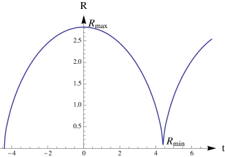
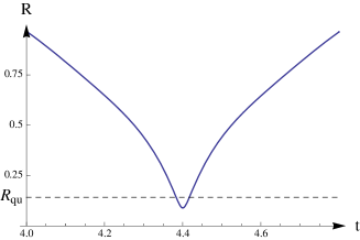
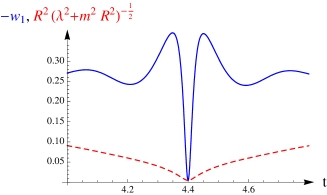
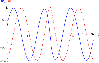
Figure 1. Quantum oscillations preventing the big crunch for $\lambda=\frac{3}{2}$, $m=10.5448$ and $w_{1}(R_{\text{max}})=-0.2675$.

The classical contraction stops on the scale $R\sim R_{\text{qu}}$, where the quantum oscillations become important. This leads to an oscillatory behavior of $R$. As a consequence, the sign of $\dot{R}$ may flip at some minimal radius $R_{\text{min}}$, where the universe again begins to expand, going over to a classical FRW-like space-time. The functions $w_{2}$ and $w_{3}$ oscillate, with slightly varying amplitude. The function $w_{1}$ is nearly constant in the classical region, but becomes oscillatory near the quantum regime $R\sim R_{\text{qu}}$ (see Figure 1); its nonlinear interplay with the scale function $R$ leads to the surprising effect that the big crunch is avoided.

The behavior in the quantum regime depends crucially on the phase $\phi$ of the Dirac oscillations, defined by $\phi=\arctan(w_{2}/w_{3})$. In Figure 2 the minimal radius $R_{\text{min}}$ is plotted as a function of the initial value of $\phi$.

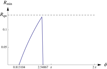
Figure 2. Dependence of the minimal radius on the initial angle $\phi$ for $\lambda=\frac{3}{2}$, $m=10.5448$ and $w_{1}(R_{\text{max}})=-0.2675$.

If $R_{\text{min}}>0$, the big crunch is avoided and $R$ “bounces back,” whereas in the case $R_{\text{min}}=0$ the big crunch appears despite the quantum effects. Considering the phase $\phi$ as unknown, one can give the result of Figure 2 a statistical interpretation: For a random initial phase, this bounce appears with a finite probability (in the example of Figure 2, this probability has the value $p=0.276224$).

Let us briefly discuss the qualitative dependence of the bounce on the free parameters $R_{\text{max}}$, $R_{\text{qu}}$, $\lambda$, and $\phi$ of our model (for a detailed analysis we refer to [4]). First of all, the probability of preventing the crunch can be increased by choosing $|w_{1}(R_{\text{max}})|$ smaller. This is shown in the example Figure 3, where the bounce occurs even with probability one.

   

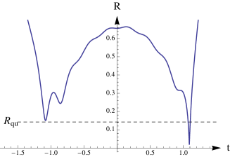
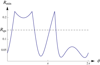
Figure 3. Quantum oscillations preventing the big crunch for $\lambda=\frac{3}{2}$, $m=10.5448$ and $w_{1}(R_{\text{max}})=-0.0608$.

We point out that small $|w_{1}(R_{\text{max}})|$ does not imply that $R_{\text{max}}$ is also small. Namely, as one sees from the Einstein equation in (9) by setting $\dot{R}$ equal to zero, a small value of $|w_{1}(R_{\text{max}})|$ can be compensated by choosing $m$ or $\lambda$ large. This leaves us the freedom to choose $R_{\text{qu}}$, (13), at will. In this way, one can construct space-times with a high probability of bouncing in the physically relevant case where $R_{\text{max}}$ is the size of our universe and $R_{\text{qu}}$ is a microscopic length scale.

An interesting limiting case of our ED equations is obtained by dropping the first summand in (10). This is a good approximation in the so-called scale dominated region where $R$ decreases so fast that the oscillations of $w_{2}$ and $w_{3}$ can be neglected. In particular, the scale dominated region describes the bounce in the physically interesting limit $R_{\text{max}}\rightarrow\infty$ (for fixed $\lambda$). In this limiting case, we can integrate the Dirac equation in (9) explicitly and express $\vec{w}$ as a function of $R$,

$$\vec{w}(t)=\begin{pmatrix}\cos\nu&0&-\sin\nu\\ 0&0&0\\ \sin\nu&0&\cos\nu\end{pmatrix}\vec{w}(t_{0})\>,$$

where $\nu(t)=-\arctan[R(t)/R_{\rm qu}]+\arctan[R(t_{0})/R_{\rm qu}]$, and $t_{0}$ is the time from which on the scale dominated approximation applies. For the probability $p$ that the crunch is avoided one obtains

$$p=\frac{1}{\pi}\>\arccos\left(\frac{|w_{1}(R_{\text{max}})|}{\sqrt{1-w_{1}(R_{\text{max}})^{2}}}\>\frac{R_{\text{qu}}}{R_{\text{max}}}\right).$$

This probability tends to $1/2$ as $R_{\rm max}$ tends to infinity, showing that the bounce is of significance even for fixed $|w_{1}(R_{\text{max}})|$ in an arbitrarily large universe.

4. Time-Periodic Solutions

By iteratively adjusting the starting values at $t=0$, we constructed time-periodic solutions. In Figure 4 an example of a time-periodic solution is shown. Except near the “quantum turning points” between collapse and expansion, the space-time is well-approximated by the classical dust-dominated FRW universe. The energy conditions are satisfied except near the quantum turning points, as is shown on the right of Figure 4. We point out that the periodic solutions were constructed by fine-tuning the initial condition and are thus not generic. A generic solution collapses after a finite number of cycles.

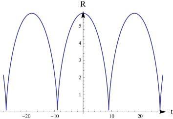
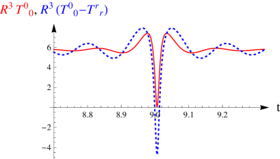
Figure 4. A time-periodic ED cosmology for $\lambda=\frac{3}{2}$, $m=21.4286$, $\vec{w}_{|t=0}=(-0.267774,0,-0.963482)$.

5. Conclusion

A new class of solutions of the Einstein equations coupled to Dirac spinors was constructed. These solutions satisfy the energy conditions except at the quantum turning points and are thus physically relevant. Our model reveals in a simple and explicit setting a general mechanism which tends to avoid space-time singularities, such as the big bang or the big crunch, if the quantum mechanical nature of matter is taken into account. By fine-tuning the initial conditions our model even allows for periodic solutions, an eternal universe with an infinite number of cycles.

Acknowledgements. We thank the referees for helpful comments. We are grateful to the Vielberth Foundation, Regensburg, for generous support. C.H. would like to thank the Erwin Schrödinger Institute, Vienna.

References

- [1] M. Bojowald, How quantum is the big bang?, arXiv:0805.1192 [gr-qc], Phys. Rev. Lett. 100 (2008), 221301.
- [2] M. Demianski, R. de Ritis, G. Platania, P. Scudarello, and C. Stornaiolo, Inflation in a Bianchi I-type Einstein-Cartan cosmological model, Phys. Rev. D 35 (1987), no. 4, 1181–1184.
- [3] F. Finster, Local symmetry in relativistic quantum mechanics, arXiv:hep-th/9703083, J. Math. Phys. 39 (1998), no. 12, 6276–6290.
- [4] F. Finster and C. Hainzl, A spatially homogeneous and isotropic Einstein-Dirac cosmology, in preparation (2011).
- [5] F. Finster, J. Smoller, and S.-T. Yau, Particlelike solutions of the Einstein-Dirac equations, arXiv:gr-qc/9801079, Phys. Rev. D (3) 59 (1999), no. 10, 104020, 19.
- [6] T. Padmanabhan and J.V. Narlikar, Quantum conformal fluctuations in a singular space-time, Nature 259 (1982), 677–678.
- [7] L. Parker and S.A. Fulling, Quantized matter fields and the avoidance of singularities in general relativity, Phys. Rev. D 7 (1974), no. 6, 2357–2374.
- [8] R. Penrose and W. Rindler, Spinors and space-time. Vol. 1, Cambridge Monographs on Mathematical Physics, Cambridge University Press, Cambridge, 1987.
- [9] A.V. Toporensky, Chaos in closed isotropic cosmological models with steep scalar field potential, Int.J.Mod.Phys. D 8 (1999), 677–678.
- [10] N. Turok, M. Perry, and P.J. Steinhardt, M theory model of a big crunch/big bang transition, arXiv:hep-th/0408083, Phys. Rev. D (3) 70 (2004), no. 10, 106004, 18.
- [11] C. Wetterich, Quintessence – the dark energy in the universe?, arXiv:astro-ph/0110211, Space Science Review 100 (2002), 195–206.