WATER, O₂, AND ICE IN MOLECULAR CLOUDS

Abstract

We model the temperature and chemical structure of molecular clouds as a function of depth into the cloud, assuming a cloud of constant density $n$ illuminated by an external FUV (6 eV $<h\nu<13.6$ eV) flux $G_{0}$ (scaling factor in multiples of the local interstellar field). Extending previous photodissociation region models, we include the freezing of species, simple grain surface chemistry, and desorption (including FUV photodesorption) of ices. We also treat the opaque cloud interior with time-dependent chemistry. Here, under certain conditions, gas phase elemental oxygen freezes out as water ice and the elemental C/O abundance ratio can exceed unity, leading to complex carbon chemistry. Gas phase H₂O and O₂ peak in abundance at intermediate depth into the cloud, roughly $A_{V}\sim 3-8$ from the surface, the depth proportional to $\ln(G_{0}/n)$. Closer to the surface, molecules are photodissociated. Deeper into the cloud, molecules freeze to grain surfaces. At intermediate depths photodissociation rates are attenuated by dust extinction, but photodesorption prevents total freezeout. For $G_{0}<500$, abundances of H₂O and O₂ peak at values $\sim 10^{-7}$, producing columns $\sim 10^{15}$ cm^-2, independent of $G_{0}$ and $n$. The peak abundances depend primarily on the product of the photodesorption yield of water ice and the grain surface area per H nucleus. At higher values of $G_{0}$, thermal desorption of O atoms from grains enhances the gas phase H₂O peak abundance and column slightly, whereas the gas phase O₂ peak abundance rises to $\sim 10^{-5}$ and the column to $\sim 2\times 10^{16}$ cm^-2. We present simple analytic equations for the abundances as a function of depth which clarify the dependence on parameters. The models are applied to observations of H₂O, O₂, and water ice in a number of sources, including B68, NGC 2024, and $\rho$ Oph.

1 INTRODUCTION

Oxygen is the third most abundant element in the universe, after hydrogen and helium, so that a basic knowledge of oxygen chemistry in molecular clouds is essential in order to understand the chemical structure, thermal balance, and diagnostic line emission from star-forming molecular gas in galaxies. Early gas-phase chemical models (e.g., Langer & Graedel 1989, Millar 1990, Bergin et al 1998) predicted large abundances of H₂O ($\sim 10^{-6}$) and O₂ ($\sim 10^{-5}-10^{-4}$) relative to hydrogen nuclei in molecular gas well shielded from far ultraviolet (FUV, 6 eV $<h\nu<13.6$ eV) photons. If gas phase H₂O and O₂ were that abundant, they would be important coolants for dense gas (Goldsmith & Langer 1978, Hollenbach 1988, Neufeld, Lepp, & Melnick 1995). However, the Submillimeter Wave Astronomy Satellite (SWAS) made pointed observations in low energy transitions of ortho-H₂O (the 1${}_{10}-1_{01}$ transition at 557 GHz) and O₂ (the 3${}_{3}-1_{2}$ transition at 487 GHz) toward numerous dense (but unshocked) molecular cores and determined that the line-of-sight-averaged and beam-averaged (SWAS beam $\sim 4^{\prime}$) abundance of H₂O is of order $\,\raise 1.29167pt\hbox{$<$}\kern-7.5pt\lower 3.01385pt\hbox{$\sim$}\,3\times 10^{-8}$ (Snell et al 2000) and that of O₂ is $\,\raise 1.29167pt\hbox{$<$}\kern-7.5pt\lower 3.01385pt\hbox{$\sim$}\,10^{-6}$ (Goldsmith et al 2000). More recent observations by the Odin mission set more stringent upper limits on O₂, $\,\raise 1.29167pt\hbox{$<$}\kern-7.5pt\lower 3.01385pt\hbox{$\sim$}\,10^{-7}$ (Pagani et al 2003), with a reported detection at the $\sim 2.5\times 10^{-8}$ level in $\rho$ Oph (Larsson et al 2007). Although the water abundance derived from the observed water emission depends inversely on the gas density, and therefore is somewhat uncertain, understanding the two order of magnitude discrepancy between the gas phase chemical models and the observations is essential to astrochemistry and to the basic understanding of the physics of molecular clouds.

Previous attempts to explain the low abundance of H₂O and O₂ observed by SWAS showed that time dependent gas-phase chemistry by itself would not be sufficient (Bergin et al 1998, 2000). Starting from atomic gas, a dense ($n(H_{2})\sim 10^{5}$ cm^-3) cloud only took $\,\raise 1.29167pt\hbox{$>$}\kern-7.5pt\lower 3.01385pt\hbox{$\sim$}\,10^{4}$ years to reach H₂O abundances $\sim 10^{-6}$, close to the final steady-state values and much greater than observed.

The best previous explanation involved time-dependent chemistry linked with the freezeout of oxygen species on grain surfaces and the formation of substantial water ice mantles on grains (Bergin et al 2000). In these models, all the oxygen in the molecular gas which is not tied up in CO adsorbs quickly (in $\sim 10^{5}$ years for a gas density of $\sim 10^{4}$ cm^-3) to grain surfaces, forms water ice and remains stuck on the grain as an ice mantle. As a result, the gas phase H₂O abundance drops from $\sim 10^{-6}$ to $\sim 10^{-8}$. The grains are assumed too warm for CO to freeze as a CO ice mantle, so that for a period from about $10^{5}$ years to about $3\times 10^{6}$ years, the gas phase H₂O abundance remains at the $\sim 10^{-8}$ level, fed by the slow dissociation of CO into O and the subsequent reaction of some of this O with H${}_{3}^{+}$, which then ultimately forms gas-phase H₂O. The slow dissociation of CO is driven by cosmic ray ionization of He; the resultant He⁺ reacts with CO to form O and C⁺. After $\sim 3\times 10^{6}$ years, even the gas phase CO abundance drops significantly as the dissociation process bleeds away the oxygen which ends up as water ice on grain surfaces. Therefore, after about $3\times 10^{6}$ years, the gas phase H₂O also drops from $\sim 10^{-8}$ to $<10^{-9}$. This previous scenario explained the observed H₂O emission as arising from the central, opaque regions of the cloud, where the abundance has dropped to the observed values but have not had time to reach the extremely low steady state values. The model relied, then, on a “tuning” of molecular cloud timescales so that they are long enough for the freeze-out of existing gas phase oxygen not in CO onto grains, but not so long that the CO is broken down and the resultant O converted to water ice, which would cause the gas phase H₂O abundances to drop below the observed values. The model also relied on CO not freezing out on grains in the opaque cloud centers.

To add to the problems of modeling the SWAS data, the SWAS team observed a number of strong submillimeter continuum sources such as SgrB, W49 and W51 and found the 557 GHz line of H₂O in absorption, as the continuum passed through translucent clouds ($A_{V}\sim 1-5$) along the line of sight (Neufeld et al 2002, Neufeld et al 2003, Plume et al 2004). The absorption measurement provided an even better estimate of the H₂O column, $N$H₂O, through these clouds because the absorption line strengths are only proportional to $N(H_{2}O)$, whereas the emission line strengths are proportional to $n(H_{2})N(H_{2}O)e^{-27{\rm K}/T}$ since the line is subthermal, effectively optically thin, and lies $\Delta E/k=27$ K above the ground state. Therefore, to obtain columns from emission line observations requires the separate knowledge of both the gas density and the gas temperature. The absorption measurements showed column-averaged abundances of H₂O of $\sim 10^{-7}-10^{-6}$ with respect to H₂, using observed CO columns and multiplying by $10^{4}$ to obtain H₂ columns. In the context of the time-dependent models with freezeout, the difference between the abundances measured in absorption compared with those measured in emission was attributed to the presumed lower gas densities in the absorbing clouds compared to the emitting clouds. Because the freezeout time depends on $n^{-1}$, it was assumed that the lower density clouds had not had time to freeze as much oxygen from the gas phase, so that gas phase H₂O abundances were higher.

A variation of this model is that of Spaans & van Dishoeck (2001) and Bergin et al (2003), where it was noticed that the water emission seemed to trace the photodissociation region (PDR, see Hollenbach & Tielens 1999), which lies on the surface ($A_{V}\,\raise 1.29167pt\hbox{$<$}\kern-7.5pt\lower 3.01385pt\hbox{$\sim$}\,5$) of the molecular cloud. A two component model was invoked in which the water froze out as ice in the dense clumps, but remained relatively undepleted in the low density interclump gas because of the longer timescales for freezeout. Thus, the average gas phase water abundance was derived from a mix of heavily depleted and undepleted gas.

We propose in this paper a new model of the H₂O and O₂ chemistry in a cloud. In this model, we assume that the molecular cloud lifetime is sufficiently long to allow freezeout and reduce the gas phase H₂O and O₂ abundances to very low values in the central, opaque regions of the cloud. The key to understanding the H₂O emission and the O₂ upper limits observed by SWAS and Odin is to model the spatially-dependent H₂O and O₂ abundances through each cloud. At the surface of the cloud the gas-phase H₂O and O₂ abundances are very low because of the photodissociation by the ISRF or by the FUV flux from nearby OB stars. Near the cloud surface the dust grains have little water ice because of photodesorption by the FUV field. Deeper into the cloud, the attenuation of the FUV field leads to a rapid rise of the gas-phase H₂O and O₂ abundances, which peak at a hydrogen nucleus column $N_{f}\sim 10^{21.5}-10^{22}$ cm^-2 (or depths $A_{Vf}\sim$ several into the cloud) and plateau at this value for $\Delta A_{V}\sim$ several beyond $A_{Vf}$, insensitive to the gas density $n$ and the incident FUV flux $G_{0}$ (scaling factor in multiples of the avearage local interstellar radiation field). At these intermediate depths, photodesorption of some of the water ice by FUV photons keeps the gas phase water abundance high (the “$f$” in $N_{f}$ and $A_{Vf}$ signifies the onset of water ice freezeout, as will be discussed in §2.5 and §3.3). The FUV is strong enough to keep some of the ice off the grains, but, due to efficient water ice formation followed by photodesorption, it is not strong enough to dissociate all gas-phase water. At greater depths, gas phase reactions other than photodissociation begin to dominate gas phase H₂O destruction, and the steady state gas phase H₂O and O₂ abundances plummet as all the gas phase elemental O is converted to water ice. Thus, the overall structure of a molecular cloud has three subregions: at the surface is a highly “photodissociated region”, at intermediate depths is the “photodesorbed region”, and deep in the cloud is the “freezeout region”.

In this new model, the H₂O and O₂ emission mainly arise from the layer of high abundance gas in the plateau which starts at $N_{f}$ and extends somewhat beyond, so that the emission is a (deep) “surface” process rather than a “volume” process. For clouds with columns $N>N_{f}$, the H₂O and O₂ emission becomes independent of cloud column, assuming the incident FUV field and gas density are fixed. The model gives column-averaged abundances through the dense cores of $\,\raise 1.29167pt\hbox{$<$}\kern-7.5pt\lower 3.01385pt\hbox{$\sim$}\,10^{-8}$ for H₂O and O₂ for low values of $G_{0}<500$, but the local abundances peak at values which are at least an order of magnitude larger than these values. For cloud columns $N>N_{f}$, the average H₂O abundance scales as $N^{-1}$.

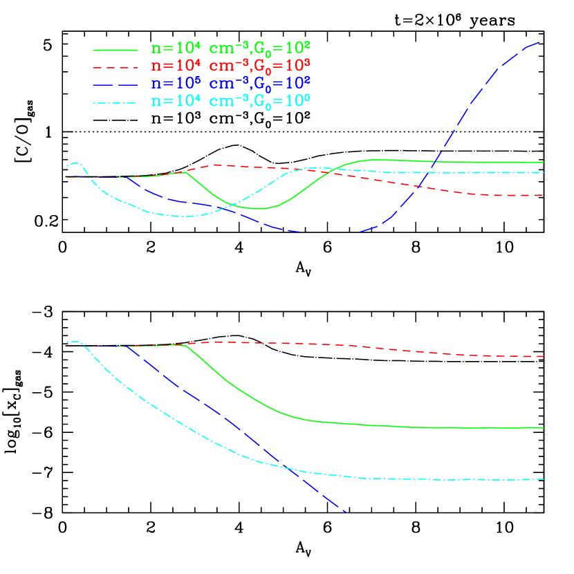
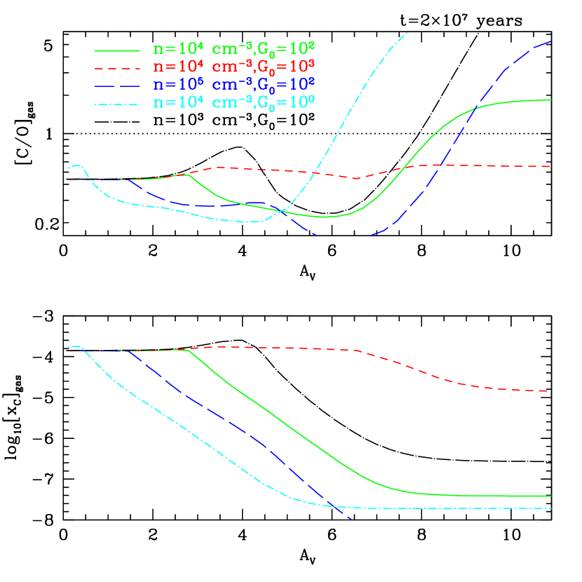
The implications of this scenario for molecular clouds may be much broader than this particular model of H₂O and O₂ chemistry in clouds. Other molecules such as CO, CS, CN, and HCN require a spatial model of their distribution in a cloud, with photodissociation and photodesorption the dominant processes near the cloud surface, and the freezing out of the molecules the dominant process deeper into the cloud. In addition, the adsorption process and creation of abundant ice mantles changes the relative gas phase abundances of the elements. In the case considered in this paper, the C/O ratio in the gas may go from 0.5 at the cloud surface to unity or greater in the H₂O freezeout region. Such changes in the gas phase C/O ratio have major implications on all gas phase chemistry (e.g., Langer et al 1984, Bergin et al 1997).

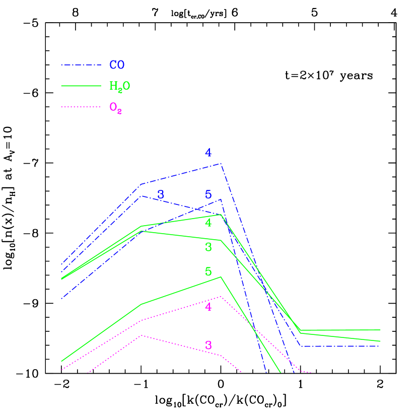
The interesting and important caveat to this relatively simple steady state model is the effect of time-dependence in raising abundances of, for example, gas phase H₂O, O₂, and CO above steady state values in the opaque ($A_{V}>5-10$) interiors of clouds. One such effect is that at low densities, $n\,\raise 1.29167pt\hbox{$<$}\kern-7.5pt\lower 3.01385pt\hbox{$\sim$}\,10^{3}$ cm^-3, species do not have time to freeze out within cloud lifetimes and therefore have much higher gas phase abundances. We have also uncovered a new time-dependent process that may elevate the H₂O and O₂ abundances for times $t\,\raise 1.29167pt\hbox{$<$}\kern-7.5pt\lower 3.01385pt\hbox{$\sim$}\,10^{7}$ years in the freezeout region at very high $A_{V}$ even at high cloud densities $n\sim 10^{5}$ cm^-3. If the grains are sufficiently cold to freeze out CO ($T_{gr}\,\raise 1.29167pt\hbox{$<$}\kern-7.5pt\lower 3.01385pt\hbox{$\sim$}\,20$ K or $G_{0}\,\raise 1.29167pt\hbox{$<$}\kern-7.5pt\lower 3.01385pt\hbox{$\sim$}\,500$) at high $A_{V}$, a CO/H₂O ice mix rapidly ($t\,\raise 1.29167pt\hbox{$<$}\kern-7.5pt\lower 3.01385pt\hbox{$\sim$}\,10^{5-6}$ years) forms. The steady state solution has very little CO ice with most of the O in H₂O ice. However, the time to convert CO ice to H₂O ice is very long, and the bottleneck is the cosmic ray desorption of CO from the CO/H₂O ice mixture. This desorption provides gas phase CO which then acts as a reservoir to produce gas phase H₂O and O₂, until all the oxygen eventually freezes out as water ice (i.e., the same mechanism as described in Bergin et al (2000) except the gas phase CO in this case comes from the CO ice). Depending on the assumptions regarding the CO desorption process, this cosmic ray CO desorption timescale may range from $10^{5}$ to $>>10^{7}$ years. If the timescale is roughly 0.1 to 1 times the cloud age, a maximum gas phase H₂O and O₂ abundance is produced at that time. Although not as large as the peak abundances produced at $A_{Vf}$, these abundances can be significant and can contribute to the total column of these species if the cloud has a high total column (but only if the CO desorption time is 0.1 to 1 times the cloud age).

This paper is organized as follows. In §2 we describe the new chemical/thermal model of an opaque molecular cloud illuminated by FUV radiation. The major changes implemented in our older photodissociation region (PDR) models (Kaufman et al 1999) include the adsorption of gas species onto grain surfaces, chemical reactions on grain surfaces, and the desorption of molecules and atoms from grain surfaces. In §3 we show the results of the numerical code as functions of the cloud gas density $n$, the incident FUV flux $G_{0}$, and the grain properties. We present a simple analytical model that explains the numerical results and how the abundances scale with depth and with the other model parameters. We discuss time dependent models for the opaque cloud center. In §4 we apply the numerical model to both diffuse clouds and dense clouds. Finally, we summarize our results and conclusions in §5. For the convenience of the reader, Table 3 in the Appendix lists the symbols used in the paper.

2 THE CHEMICAL AND THERMAL MODEL OF AN OPAQUE MOLECULAR CLOUD

2.1 Summary of Prior PDR Model and Modifications

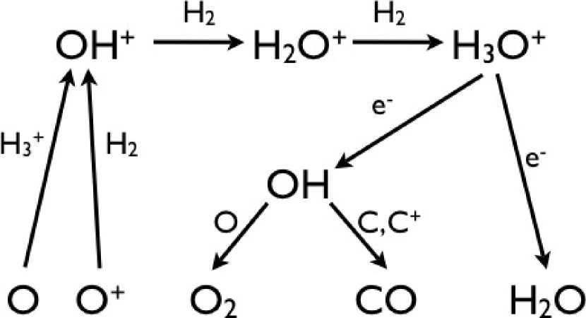
The numerical code we have developed to model the chemical and thermal structure of an opaque cloud externally illuminated by FUV flux is based on our previous models of photodissociation regions (PDRs), which are described in Tielens & Hollenbach (1985), Hollenbach et al (1991), and Kaufman et al (1999,2006). This 1D code modeled a constant density slab of gas, illuminated from one side by an FUV flux of $1.6\times 10^{-3}G_{0}$ erg cm^-2 s^-1. The unitless parameter $G_{0}$ is defined above in such a way that $G_{0}\sim 1$ corresponds to the average local interstellar radiation field in the FUV band (Habing 1968). The subscript “0” indicates that the flux is the incident FUV flux, as opposed to the attenuated FUV flux deeper into the slab. The code calculated the steady state chemical abundances and the gas temperature from thermal balance as a function of depth into the cloud. It incorporated $\sim 45$ chemical species, $\sim 300$ chemical reactions, and a large number of heating mechanisms and cooling processes. The chemical reactions included FUV photoionization and photodissociation; cosmic ray ionization; neutral-neutral, ion-neutral, and electronic recombination reactions, including reactions with charged dust grains; and the formation of H₂ on grain surfaces. No other grain surface chemistry was included in these prior models. The main route to gas phase H₂O and O₂ through these gas-phase reactions is schematically shown in Fig. 1. It starts with the ionization of H₂ by cosmic rays or X-rays, which eventually leads to H₃O⁺ that recombines to form gas phase water. It also recombines to form OH which reacts with O to form gas phase O₂. The code contained a relatively limited carbon chemistry; we included CH and CH₂, as well as their associated ions, but did not include CH₃, CH₄, C₂H or longer carbon chains, nor any carbon molecules that include S or N.

The code modeled regions which lie at hydrogen column densities $N\,\raise 1.29167pt\hbox{$<$}\kern-7.5pt\lower 3.01385pt\hbox{$\sim$}\,2\times 10^{22}$ cm^-2 (or $A_{V}\,\raise 1.29167pt\hbox{$<$}\kern-7.5pt\lower 3.01385pt\hbox{$\sim$}\,10$) from the surface of a cloud. Therefore, it applied not only to the photodissociated surface region, where gas phase hydrogen and oxygen are nearly entirely atomic and where gas phase carbon is mostly C⁺, but also to regions deeper into the molecular cloud where hydrogen is in H₂ and carbon is in CO molecules. Even in these molecular regions, the attenuated FUV field can play a significant role in photodissociating H₂O and O₂, and in heating the gas.

The dust opacity is normalized to give the observed visual extinction per unit H nucleus column density that is observed in the diffuse ISM (e.g., Savage & Mathis 1979, Mathis 1990). The extinction in the FUV, assumed to go as $e^{-b_{\lambda}A_{V}}$, is taken from PDR models described most recently in Kaufman et al (1999, 2006), and mainly derived from the work of Roberge et al (1991). Here $b_{\lambda}$ is the scale factor which expresses the increase in extinction as one moves from the visual to shorter wavelengths. However, the FUV extinction law in molecular clouds is not well known. We discuss in §3.2 how our results would vary if $b_{\lambda}$ varies.

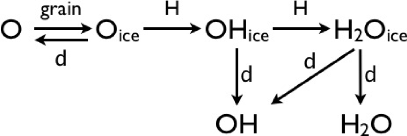
In the following subsections (§2.2 - §2.7) we describe the modifications to the basic PDR code which we have made to properly model the gas phase H₂O and O₂ abundances from the surfaces of molecular clouds to the deep interiors, where the gas phase elemental oxygen freezes out as water ice mantles on grain surfaces. The modifications include the freezeout of gas phase species onto grains, the formation of OH and H₂O as well as CH, CH₂, CH₃ and CH₄ on grain surfaces, and various desorption processes of species from grain surfaces. Fig. 2 shows the grain surface formation process for water ice.

One key modification is the application of time dependent chemistry to the deep, opaque interior. Here, certain chemical timescales are comparable to cloud lifetimes, and steady state chemical networks such as our PDR code do not apply. The time dependent code also increases the number of reactions and species we follow, and this particularly improves the treatment of the carbon chemistry in the cloud interior. Further discussion is found in §2.3, 2.4 and 3.7.

2.2 Dust Properties

The basic PDR code implicitly assumed a “MRN” (Mathis, Rumpl & Nordsieck 1977) grain size distribution $n_{gr}(a)\propto a^{-3.5}$, where $a$ is the grain radius, extending from very small ($\,\raise 1.29167pt\hbox{$<$}\kern-7.5pt\lower 3.01385pt\hbox{$\sim$}\,10$ Å) polycyclic aromatic hydrocarbons (PAHs) to large ($\sim 0.25$ $\mu$m) dust grains. With this distribution the largest grains provide the bulk of the grain mass, and the intermediate-sized grains ($\sim 100$ Å) provide the bulk of the FUV extinction. The smallest particles and PAHs provide the bulk of the surface area, and dominate the grain photoelectric heating process and the formation of H₂ on grain surfaces. The code implicitly assumes an MRN distribution in the sense that the equations for attenuation of incident photons by dust, for grain photoelectric heating, for H₂ formation, and for gas-grain collisions and the charge transfer that may occur in such collisions all assume such a distribution.

For the process of the freezeout of oxygen species onto grain surfaces, we also implicitly assume an MRN distribution, in the sense that we adopt a cross sectional grain area $\sigma_{H}$ appropriate for an MRN distribution. As will be shown in §3, $\sigma_{H}$, which is one fourth the surface area available for freezeout, is an important parameter for determining the abundance of gas-phase $\rm H_{2}O$ in our models. Below in §2.5, we show that $\sigma_{H}$ is roughly the total cross sectional area of grains (per H) that are larger than about 20 Å. Smaller grains experience single photon heating events which clear them of ice mantles (Leger, Jura, & Omont 1985). In addition, cosmic rays may clear small grains of ices (Herbst & Cuppen 2006). In an MRN distribution, the cross sectional area of grains with radii larger than about 20 Å is $\sigma_{H}\sim 2\times 10^{-21}$ cm² per H.

We note, however, that the cross sectional area is somewhat uncertain. It could be smaller if grains coagulate inside of dense molecular clouds. It could be larger due to ice buildup. We note that once all oxygen-based ices freeze out onto such an MRN distribution, it forms a constant mantle thickness of $\Delta a\sim 50$ Å regardless of grain size. While this is insignificant to the large ($\sim 0.1$ $\mu$m) grains which contain most of the mass, it represents a very large change in radius and area of the smallest ($\sim 20$ Å) grains which provide most of the grain surface area. The increased surface area of grains at the end of this freezeout will proportionally increase subsequent gas-grain interaction rates. Thus, neutralization of ions by grains, formation of H₂ on grain surfaces, the freezeout of species, and the cooling or heating of the gas by gas-grain collisions may all be enhanced by significant amounts in regions where water ice has totally frozen out on grains. However, because of the possibility of grain coagulation which reduces grain surface area, and because of the uncertainly in the lower size cutoff of effective grains, we have chosen to fix $\sigma_{H}$ and treat it as a (constrained) variable with values ranging from $\sigma_{H}=6\times 10^{-22}$ to 6 $\times 10^{-21}$ cm² per H.

2.3 Adsorption and Time Dependent Chemistry

Adsorption is the process by which a gas phase atom or molecule hits a grain and sticks to the surface due to van der Waals or stronger surface bonding forces. Typically, at the low gas temperatures we will consider, $T_{gas}\,\raise 1.29167pt\hbox{$<$}\kern-7.5pt\lower 3.01385pt\hbox{$\sim$}\,50$ K, the sticking probability is of order unity for most species (Burke & Hollenbach 1983). We assume unit sticking coefficients here for all species heavier than helium. Thus, the timescale to adsorb (freeze) is the timescale for a species to strike a grain surface:

$$t_{f,i}\sim[n_{gr}\sigma_{gr}v_{i}]^{-1},$$ (1)

where $v_{i}$ is the thermal speed of species $i$ and where the grain number density $n_{gr}$ times the grain cross section $\sigma_{gr}$ is the average over the size distribution. As discussed above, in an MRN distribution with a lower cutoff size of $a\sim 20$ Å, $n_{gr}\sigma_{gr}\simeq 2\times 10^{-21}n$ cm^-1, where $n$ is the gas phase hydrogen nucleus density in units of cm^-3. Therefore, $t_{f,i}\sim 8\times 10^{4}(m_{O}/m_{i})^{1/2}(10^{4}{\rm cm^{-3}}/n)(30{\rm K}/T)^{1/2}$ years, where $m_{O}$ is the mass of atomic O and $m_{i}$ is the mass of the species. Since molecular cloud lifetimes are thought to be $2\times 10^{6}$ to $2\times 10^{7}$ years, and the molecules reside in regions with $n\,\raise 1.29167pt\hbox{$>$}\kern-7.5pt\lower 3.01385pt\hbox{$\sim$}\,10^{3}$ cm^-3, this short timescale suggests that molecules should mostly freeze out in molecular clouds unless some process desorbs them from grains. Dust vacuums the condensibles quickly!

Consider the depletion of CO in regions where the grain temperatures are too high to directly freeze out CO. CO freezes out when grain temperatures are $T_{gr}\,\raise 1.29167pt\hbox{$<$}\kern-7.5pt\lower 3.01385pt\hbox{$\sim$}\,20$ K (see §2.4 below). However, H₂O freezes out when grain temperatures are $T_{gr}\,\raise 1.29167pt\hbox{$<$}\kern-7.5pt\lower 3.01385pt\hbox{$\sim$}\,100$ K at the densities in molecular clouds. Suppose that 20 K$<T_{gr}<100$ K, so that gas phase elemental oxygen not in CO freezes out as water ice, but CO does not directly freeze. CO is continuously destroyed by He⁺ ions created by cosmic rays, producing C⁺ and O. The resultant O has two basic paths: it can reform CO, or it can freeze out on grain surfaces as water ice, never to return to the gas phase in the absence of desorption mechanisms. The latter process therefore slowly depletes the CO gas phase abundance, by lowering the available gas phase elemental O. We see this effect in the late time evolution of CO in Bergin et al (2000). One effect, not included in Bergin et al, that slows this process is that for grain temperatures $\,\raise 1.29167pt\hbox{$>$}\kern-7.5pt\lower 3.01385pt\hbox{$\sim$}\,20$ K adsorbed atomic O may be rapidly thermally desorbed before reacting with H and therefore the production of H₂O ice by grain surface reactions may be substantially curtailed (this will be discussed further in §2.5 and §3.2). Nevertheless, gas phase H₂O will form and will freeze out, and therefore, given enough time, the elemental O not incorporated in refractory (e.g., silicate) grain material is converted to H₂O ice. If elemental C does not evolve to a similarly tightly bound carbonaceous ice, there is the potential for the gas phase C/O number ratio to exceed unity. This will have consequences for astrochemistry (e.g., Langer et al 1984, Bergin et al 1997, Nilsson et al 2000), and we show some exemplary results in §3.5.

Consider as well the case where $T_{gr}\,\raise 1.29167pt\hbox{$<$}\kern-7.5pt\lower 3.01385pt\hbox{$\sim$}\,20$ K deep in the cloud (i.e., at $A_{V}>5$; this low $T_{gr}$ corresponds to $G_{0}\,\raise 1.29167pt\hbox{$<$}\kern-7.5pt\lower 3.01385pt\hbox{$\sim$}\,500$). In this case, the gas phase CO freezes out with the H₂O, forming a CO/H₂O ice mix. In order for this CO ice to be converted to H₂O ice, the CO needs to be desorbed by cosmic rays. It then reacts in the gas phase with He⁺ as described above and eventually the freed O goes on to form mostly water ice. The timescale for this CO cosmic ray desorption can be quite long, and may dominate the slow evolution of the chemistry toward steady state.

Unfortunately, this timescale is not well known. First of all, cosmic ray desorption rates are not well constrained. But secondly, the timescales depend on the structure of the CO/H₂O ice mix, and this structure is not certain. If the molecules are immobile, the CO and H₂O ice molecules are initally mixed and each monolayer contains this mix. However, there is some evidence that either pure CO ice pockets form, or the CO accretes on top of an already formed layer of water ice (Tielens et al 1991, Lee et al 2005, Pontoppidan et al 2004, 2008). Even if the CO and H₂O are initially mixed and immobile, cosmic rays desorb CO much more efficiently than H₂O due to the much smaller binding energy of adsorbed CO compared with adsorbed H₂O (Leger, Jura, & Omont 1985). This could lead to surface monolayers with very little CO compared to the protected layers underneath the surface. The cosmic ray desorption rate is directly proportional to the fraction of surface sites occupied by CO. In the examples above, this fraction could range from zero to unity. Thus, the desorption timescale could range from large values ($>>10^{7}$ years) to small values ($\sim 10^{5}$ years). We compute these timescales in §2.4.

Because of the moderately long timescale for the depletion of either gas phase or ice phase CO via this freezing out of the elemental O in the form of water ice, we apply time dependent chemical models (see §3.7) to the cloud interiors which are run for the presumed lifetimes ($\sim 10^{7}$ years) of molecular clouds. Time dependent models are also warranted for clouds of relatively low density, $n\,\raise 1.29167pt\hbox{$<$}\kern-7.5pt\lower 3.01385pt\hbox{$\sim$}\,10^{3}$ cm^-3, where $t_{f}\,\raise 1.29167pt\hbox{$>$}\kern-7.5pt\lower 3.01385pt\hbox{$\sim$}\,2\times 10^{6}$ years (see Eq. 1).

2.4 Desorption

To desorb a species from a grain surface requires overcoming the binding energy which holds the species to the surface. Table 1 lists the binding energies of the key species we treat. Note that water has a very high binding energy and is therefore more resistant to desorption.

Thermal Desorption. The rate $R_{td,i}$ per atom or molecule of thermal desorption from a surface can be written:

$$R_{td,i}\simeq\nu_{i}e^{-E_{i}/kT_{gr}},$$ (2)

where $E_{i}$ is the adsorption binding energy of species $i$ and $\nu_{i}=1.6\times 10^{11}\sqrt{(E_{i}/k)/(m_{i}/m_{\rm H})}$ s^-1 is the vibrational frequency of the species in the surface potential well, $k$ is Boltzmann’s constant and $m_{i}$ and $m_{H}$ are the mass of species $i$ and hydrogen, respectively. One can find the temperature at which a species freezes by equating the flux $F_{td,i}$ of desorbing molecules from the ice surface to the flux of adsorbing molecules from the gas,

$$F_{td,i}\equiv N_{s,i}R_{td,i}f_{s,i}=0.25n_{i}v_{i},$$ (3)

where $N_{s,i}$ is the number of adsorption sites per cm² ($N_{s,i}\sim 10^{15}$ sites cm^-2), $f_{s,i}$ is the fraction of the surface adsorption sites that are occupied by species $i$, $n_{i}$ is the gas phase number density of species $i$ and $v_{i}$ is its thermal speed. We have assumed sticking probability of unity. From these equations, one can calculate the freezing temperature $T_{f,i}$ of a species by solving for $T_{gr}$.

$$T_{f,i}\simeq(E_{i}/k)\left[\ln\left({{4N_{s,i}f_{s,i}\nu_{i}}\over{n_{i}v_{i}}}\right)\right]^{-1}$$ (4)

$$T_{f,i}\simeq(E_{i}/k)\left[57+\ln\left[\left({N_{s,i}\over{10^{15}\ {\rm cm^{-2}}}}\right)\left({\nu_{i}\over{10^{13}\ {\rm s^{-1}}}}\right)\left({{1\ {\rm cm^{-3}}}\over n_{i}}\right)\left({{10^{4}\ {\rm cm\ s^{-1}}}\over v_{i}}\right)\right]\right]^{-1}.$$ (5)

This equation shows that at molecular cloud conditions the freezing temperature $T_{f,i}$ is about $0.02E_{i}/k$, or about 100 K for H₂O but only $\sim 20$ K for CO (see Table 1) We include thermal desorption rates from our surfaces as given by these equations. We compute the number of layers of an adsorbed species on the grain, and only thermally desorb from the surface layer.

Photodesorption. The flux $F_{pd,i}$ of adsorbed particles leaving a surface due to photodesorption is given by

$$F_{pd,i}=Y_{i}F_{FUV}f_{s,i},$$ (6)

where $Y_{i}$ is the photodesorption yield for species $i$, averaged over the FUV wavelength band, and $F_{FUV}$ is the incident FUV photon flux on the grain surface. We write the FUV photon flux at a depth $A_{V}$ into the cloud as (see Tielens & Hollenbach 1985)

$$F_{FUV}=G_{0}F_{0}e^{-1.8A_{V}},$$ (7)

where $F_{0}\simeq 10^{8}$ photons cm^-2 s^-1 is approximately the local interstellar flux of 6eV–13.6eV photons and $G_{0}$ is the commonly used scaling factor (see §2.1).

Reliable photodesorption yields are often hard to find in the literature, but for the case of H₂O a laboratory study has been done for the yield created by Lyman $\alpha$ photons (Westley et al 1995a, b). The mass loss at large photon doses is proportional to the photon flux, showing that desorption is not due to sublimation caused by absorbed heat. The yield is negligible when infrared or optical photons are incident. As an approximation, we will assume the average yield in the FUV (912-2000 Å) is the same as the Lyman $\alpha$ (1216 Å) yield. Most of the photodesorption occurs when the incident photon is absorbed in the first two surface monolayers of the water ice (Andersson et al 2006). The value of the yield ($\sim 1-8\times 10^{-3}$) is perhaps 10 times smaller than the probability that the incident photon is absorbed in the first two surface monolayers, so the photodesorption efficiency from these layers is of order 10%. We note that this yield from Westley et al is similar to the values that Öberg (private communication) has found in preliminary experiments with a broad band FUV source.

One peculiar result from the Westley et al experiments is that the yield first increases with the dose of photons, until it hits a saturation value for that flux. The saturation dose is of order 3 $\times 10^{18}$ photons cm^-2. In the fields we are considering, $G_{0}\sim 1-10^{5}$, this dose is achieved in less than 1000 years. Thus, our grains may well be saturated. The interpretation of the increase of the photodesorption yield with dose is that photolysed radicals like O, H and OH build up on the surface to a saturation value. Chemical reactions of a newly-formed radical with a pre-existing radical may lead to the desorption of the product (usually H₂O) and explain the dose dependence of the yield. Adding further weight to this interpretation is that the saturated yields decline with decreasing surface temperature ($Y_{H_{2}O}$ is 0.008 at $T_{gr}=100$ K, 0.004 at 75 K, and 0.0035 at 35 K). As temperatures decrease the radicals cannot diffuse across the surface as well to react with other radicals, nor can activation bonds be as easily overcome. Since presumably radicals like O, H and OH are being created, and it is the process of reforming more stable molecules that may help initiate desorption–and may kick off neighboring molecules, other molecules may desorb such as OH, H, O₂, H₂. These are indeed observed, but Westley et al report that most of the desorbing molecules are water molecules. We note, however, a recent theoretical calculation by Andersson et al (2006) which suggests that one might expect OH and H to be major desorption products, but confirming that the yield of H₂O photodesorption may still be of order 10^-3. We also find (see §4.1 below) that adopting a yield for OH+H photodesorption from water ice which is twice that of H₂O photodesorption provides better agreement to the OH/H₂O abundance ratio measured in translucent clouds. We define $Y_{OH,w}$ as the yield of OH photodesorbing from water ice; $Y_{OH,w}=2Y_{H_{2}O}$. This distinguishes $Y_{OH,w}$ from $Y_{OH}$, which is the yield of OH photodesorbing from a surface covered with adsorbed OH molecules.

The interpretation that radical formation in the surface layer is important in creating photodesorption leads one to re-examine the issue of whether grains near the surfaces of molecular clouds will indeed be saturated with radicals on their surfaces. While it is true that the photon dose is sufficient, this dose was delivered over a long timescale. Westley et al (1995b) point out that it is possible in this case that radicals may recombine in the time between photon impacts within an area of molecular dimensions ($\sim 10^{-15}$ cm²), which might result in smaller yields than the saturated ones.

In light of the uncertainties in the wavelength dependence of the yield over the FUV range, the photodesorption products, and the level of saturation, we adopt $Y_{H_{2}O}=10^{-3}$ and $Y_{OH,w}=2\times 10^{-3}$ as our “standard” values, but we will show models in which these yields are varied by a factor of 10 from their standard values, maintaining their ratio of 0.5. We will also use the observations of $A_{V}$ thresholds for water ice formation to constrain the absolute values of these yields (§4.2.1), and the observations of OH and H₂O in diffuse clouds to help determine their ratio (§4.1).

Recent laboratory measurements of CO photodesorption imply a yield similar to that for H₂O (Öberg et al 2007). Therefore, we adopt $Y_{CO}=10^{-3}$ as our standard value for CO. Unless $T_{gr}<20$ K, adsorbed CO is anticipated to be rare because it thermally desorbs so rapidly. However, in cases with low $G_{0}$, CO may occupy $\sim 1/3$ of the surface sites at the H₂O freezeout column.

For the other species there is less or no reliable photodesorption data in the literature. Since our grain surface is largely H₂O ice, and the photodesorption is via the production of radicals (and possibly the reformation of H₂O from radicals), we assume that the yield for O is $Y_{O}=10^{-4}$ (a smaller yield since no reformation possible). The yields for O, OH and O₂ are less important, because in our models they rarely occupy many of the surface sites. The first two are rare because they rapidly react with H to form H₂O. Table 1 lists the photodesorption yields we adopted.

A complication arises if grains move rapidly from surface regions (higher temperature and possible lower density) where H₂O ice can exist to deeper (lower temperature and higher density) regions where CO ice forms and then back again to the surface region. The fraction of the surface now covered by H₂O ice, $f_{s,H_{2}O}$, is now nearly zero, since CO covers the surface. Therefore, H₂O and OH photodesorption rates are very low. We have ignored this effect, assuming a mix of CO and H₂O ice in each adsorbed monolayer. In this paper the region where H₂O and OH photodesorption are important is the intermediate or “plateau” region where gas phase H₂O and OH abundances peak. Here, the photodesorption and/or thermal desorption timescales of CO are much shorter than the dynamical timescales to bring CO-coated ice grains from the deep interior to the plateau region.

Desorption by Chemical Reaction. There have been some attempts to model the desorption of molecules due to chemical reactions on grain surfaces. D’Hendecourt et al (1982) and Tielens & Allamandola (1987) discuss an exploding grain hypothesis in which the UV photons produce radicals in the grains, which are relatively immobile until the grain temperature is increased. At this point, they begin to diffuse and react, and the chemical heat causes a chain reaction exploding the grain and “desorbing” species in large bursts. Our photodesorption is a sort of steady state version of this. O’Neill, Viti, & Williams (2002) examine the effects of hydrogenation on grain surfaces, and in some of their models they assume that the reaction of a newly adsorbed H atom with radicals on the surface such as OH will release enough energy to desorb the resultant hydrogenated molecule. In this case, it is the chemical energy carried in by the H atom, and not the photodissociation of the ice itself, which leads to desorption. In our standard case we assume that H₂ desorbs on formation because of its low adsorption binding energy and its low mass, but that other forming molecules do not. However, we ran one case (see §3.5) in which we include this desorption process for all forming molecules in our grain surface chemistry.

Desorption by Cosmic Rays and X-rays. Deep in the cloud, cosmic ray desorption of ices becomes important for maintaining trace amounts of O-based and C-based species in the gas phase. Cosmic ray desorption rates per surface molecule (i.e., molecule in the top monolayer of ice) for various species are listed in Table 1. As discussed above, the desorption rates depend on the abundance of a particular adsorbed species in the surface monolayer. In our standard steady state models, we assume that if there are a number of species (e.g., CO, CH₄, H₂O) that are adsorbed, that they are well mixed and each monolayer of ice contains the same mix. However, as discussed above, for CO the fraction of the surface layer containing CO may range from zero to unity. The timescale for the cosmic ray desorption of a species $i$ is given:

$$t_{cr,i}={{x(i)}\over{4R_{cr,i}N_{s,i}f_{s,i}\sigma_{H}}},$$ (8)

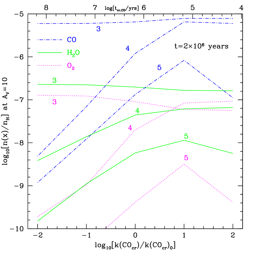
where $x(i)$ is the abundance of the adsorbed ice species and $R_{cr,i}$ is the cosmic ray desorption rate per surface atom or molecule and is given in Table 1. The cosmic ray desorption time for H₂O_ice is long ($\sim 10^{10}$ years) and is not significant in our models. However, the timescale for CO desorption under certain circumstances may be comparable to the age of the cloud, and can therefore lead to a source of gas phase CO which can then serve as a source of gas phase H₂O and O₂, as discussed above. Substituting from Table 1 for $R_{cr,CO}$, assuming an initially high abundance of CO ice, $x(CO_{ice})=10^{-4}$, and taking $f_{s,CO}=0.3$, we obtain $t_{cr,CO}\sim 2.3\times 10^{6}$ years. However, both $R_{cr,CO}$ and $f_{s,CO}$ are uncertain. In the case of the fractional surface coverage $f_{s,CO}$, the cosmic ray desorption process itself, acting on the top monolayer, could result in a very low value of $f_{s,CO}$ by essentially purging the surface of CO and leaving a fairly pure monolayer of H₂O_ice (see §2.3). On the other hand, there may be evidence for a non-polar CO ice surface on top of a polar H₂O ice mantle resulting in $f_{s,CO}=1$ (see §2.3). Because of the uncertainly in the product $f_{s,CO}R_{cr,CO}$ we will examine in §3.7 a range of values of this parameter extending from $10^{-15}$ to $10^{-11}$ s^-1. The corresponding timescale to remove all the ice is about $3\times 10^{5}$ to $3\times 10^{9}$ years, ranging from less than to much greater than cloud ages.

Cosmic rays also lead to the production of FUV photons (Gredel et al. 1989) at a level equivalent to $G_{0}\sim 10^{-3}$ throughout the cloud. We include this flux in determining both the photodissociation of gas-phase molecules and the photodesorption of ices.

Following Leger, Jura, & Omont (1985) we assume that, in general, cosmic ray desorption dominates over X-ray desorption and we therefore ignore this process. Of course, in regions close to X-ray sources and where the UV is shielded by dust, X-ray desorption will become more significant.

2.5 Timescales Related to Freezeout

Several timescales are needed to understand the freezing process fully. Assuming that the grain size distribution extends to very small grains (or large molecules) whose size is of order a few Angströms, we first compute timescales relevant for single photons to clear grains of ice due to transient heating by the photon. The peak temperature that a silicate grain of radius $a$ achieves after absorbing a typical $\sim 10$ eV FUV photon is given (Drapatz & Michel 1977, Leger, Jura & Omont 1985)

$$T_{max}\sim 100\left({{20\ {\rm\AA}}\over a}\right)^{1.3}\ {\rm K}.$$ (9)

The timescale for this grain to radiate away the energy of this photon is

$$t_{r}\sim 100\left({{100\ {\rm K}}\over T_{max}}\right)^{5}\left({{20\ {\rm\AA}}\over a}\right)^{3}\ {\rm seconds}.$$ (10)

On the other hand, the timescale for a single H₂O molecule to thermally evaporate from an ice surface on the grain is given

$$t_{evap,H_{2}O}\sim 4\times 10^{-13}e^{{4800\ {\rm K}}\over T_{max}}\ {\rm seconds},$$ (11)

where $\Delta E/k=4800$ K is the binding energy of the H₂O molecule (Fraser et al 2001) and $4\times 10^{-13}$ seconds is the period of one vibration of the molecule in the ice lattice (see Eqn 2. and following text). For comparison with the above equations, $t_{evap,H_{2}O}\simeq 10^{29}$ seconds at $T_{max}=50$ K, $3\times 10^{8}$ seconds at $T_{max}=100$ K, and 30 seconds at $T_{max}=150$ K. Comparison with $t_{r}$ indicates that the ice mantle will evaporate before cooling when $T_{max}\sim 150$ K. Comparison with the equation for $T_{max}$ shows that $a\,\raise 1.29167pt\hbox{$>$}\kern-7.5pt\lower 3.01385pt\hbox{$\sim$}\,15-20$ Å is required for grains to be large enough such that single photon events do not clear ice mantles. Thermal evaporation of H₂O will also cool the grain. Since the binding energy of an H₂O molecule is $\sim 0.5$ eV, $\sim 20$ H₂O molecules must evaporate to offset the heating due to the absorption of a single UV photon. However, we show below that 10 eV photons are absorbed by 20 Å grains more rapidly than O atoms hit the grains to form ice. Therefore, thermal evaporation cannot significantly cool the transiently heated grains compared with radiative cooling, and an entire ice mantle never builds up on the grain surface. The conclusion holds that $a\,\raise 1.29167pt\hbox{$<$}\kern-7.5pt\lower 3.01385pt\hbox{$\sim$}\,20$ Å  grains lose their ice in the presence of single photon heating events. In summary, for the purposes of modeling oxygen freezeout and ice formation, we assume that the effective surface area for ice freezeout is given by the area of grains that are larger than $\sim 20$ Å.

Several more timescales reveal the fate of an oxygen atom once it sticks to a grain. The timescale $t_{gr,O}$ for a given grain of radius $a$ to be hit by a gas phase oxygen atom is given

$$t_{gr,O}\sim 2.5\times 10^{4}\left({10^{-4}\over x(O)}\right)\left({{10\ {\rm K}}\over T_{gas}}\right)^{1/2}\left({{0.1\mu\rm m}\over a}\right)^{2}\left({{10^{5}\ {\rm cm}^{-3}}\over n}\right)\ {\rm seconds},$$ (12)

where $x(O)$ is the gas phase abundance of atomic oxygen relative to hydrogen. Similarly, the timescale $t_{gr,H}$ for the same grain to be hit by a hydrogen atom from the gas is given

$$t_{gr,H}\sim 6.0\times 10^{-1}x(H)^{-1}\left({{10\ {\rm K}}\over T_{gas}}\right)^{1/2}\left({{0.1\mu\rm m}\over a}\right)^{2}\left({{10^{5}\ {\rm cm}^{-3}}\over n}\right)\ {\rm seconds},$$ (13)

where $x(H)$ is the abundance of atomic hydrogen. Note that at the column or $A_{V}$ into the cloud where water begins to freeze out on grain surfaces, $x(H)$ is likely less than unity because most H is in H₂. However, if $x(H)\,\raise 1.29167pt\hbox{$>$}\kern-7.5pt\lower 3.01385pt\hbox{$\sim$}\,0.25x(O)$, then H atoms stick more frequently than O atoms. Provided photodesorption or thermal desorption does not intervene, and assuming that the H atoms are quite mobile on the surface and find the adsorbed O atom, O atoms will react with H atoms on the surface to form OH and then H₂O.

These timescales need to be compared to the timescale for UV photons to photodesorb the O atom and the timescale for O atoms to thermally desorb from grains. The timescale for a grain of size $a$ $\,\raise 1.29167pt\hbox{$>$}\kern-7.5pt\lower 3.01385pt\hbox{$\sim$}\,100$ Å to absorb an FUV photon is given by:

$$t_{\gamma}\sim 30G_{0}^{-1}e^{1.8A_{V}}\left({{0.1\mu\rm m}\over a}\right)^{2}\ {\rm seconds}.$$ (14)

The timescale to photodesorb an O atom from a surface covered with a covering fraction $f_{s,O}$ of O atoms is then,

$$t_{\gamma-des}\sim 3\times 10^{5}G_{0}^{-1}e^{1.8A_{V}}f_{s,O}^{-1}\left({{0.1\mu\rm m}\over a}\right)^{2}\left({Y_{O}\over 10^{-4}}\right)^{-1}\ {\rm seconds},$$ (15)

where $Y_{O}$ is the photodesorption yield for atomic O. The timescale for thermal desorption of an O atom on a grain is given

$$t_{evap,O}\sim 9\times 10^{-13}e^{{800\ {\rm K}}\over T_{max}}\ {\rm seconds}.$$ (16)

Therefore, the timescale for thermal evaporation of an O atom is $10^{22}$ seconds for a 10 K grain, $2\times 10^{5}$ seconds for a 20 K grain, and 0.3 seconds for a 30 K grain. From Eqs (12-16) one concludes that if grains are cooler than about 20-25 K and if $x(H)>0.25x(O)$, an adsorbed O atom will react with H to form OH and then H₂O before it is thermally desorbed. Photodesorption of O never appears to be important.

In this paper we are mainly interested in the abundance of gas phase H₂O and O₂ at the point where oxygen species start to freeze out in the form of water ice. This “freezeout depth” $A_{V}\equiv A_{Vf}$ is where the gas phase oxygen abundance plummets and most oxygen is incorporated as water ice on grain surfaces. This occurs when the rate at which relatively undepleted gas phase oxygen atoms hit and stick to a grain equals the photodesorption rate of water molecules from grain surfaces completely covered in ice, or $t_{\gamma-des}(A_{Vf})\sim t_{gr,O}(A_{Vf})$. Using Eqs.(12 and 15) and taking $Y\equiv Y_{OH,w}+Y_{H_{2}O}$ as the total yield of photodesorbing water ice, we find

$$A_{Vf}\simeq 0.56\ln\left[0.8G_{0}\left({Y\over 10^{-3}}\right)\left({{10\ {\rm K}}\over T_{gas}}\right)^{1/2}\left({{10^{5}\ {\rm cm}^{-3}}\over n}\right)\right],$$ (17)

if the term in brackets exceeds unity. If it is less than unity, there is freezeout at the surface of the cloud. As can be seen in Eq. (17), freezeout at the surface only occurs for very low values of $G_{0}/n\,\raise 1.29167pt\hbox{$<$}\kern-7.5pt\lower 3.01385pt\hbox{$\sim$}\,10^{-5}$ cm³.

At $A_{Vf}$ the timescale $t_{\gamma f}$ for a grain of size $a$ to absorb an FUV photon can be written, substituting Eq. (17) for $A_{Vf}$ into Eq. (14),

$$t_{\gamma f}\sim 24\left({{10\ {\rm K}}\over T_{gas}}\right)^{1/2}\left({{0.1\mu\rm m}\over a}\right)^{2}\left({{10^{5}\ {\rm cm}^{-3}}\over n}\right)\left({Y\over 10^{-3}}\right)\ {\rm seconds}.$$ (18)

As discussed above, $t_{\gamma f}<<t_{gr,O}$, so that, at this critical depth, no ice forms on small ($\,\raise 1.29167pt\hbox{$<$}\kern-7.5pt\lower 3.01385pt\hbox{$\sim$}\,20$ Å) grains because single photons can thermally evaporate adsorbed O, OH or H₂O before thermal radiative emission cools the grain and before another O atom sticks to the grain. Although ice may not form on $a\,\raise 1.29167pt\hbox{$<$}\kern-7.5pt\lower 3.01385pt\hbox{$\sim$}\,20$ Å grains, they may still contribute to the formation of gas phase OH or H₂O. Note that once an O atom sticks to a given grain, the timescale $t_{gr,H}$ for an H atom to stick (Eq. 13) may be shorter than the timescales $t_{\gamma f}$ for a photon to be absorbed. Thus, the O may be transformed into H₂O on the grain surface before a photon transiently heats the small grain and thermally evaporates the H₂O to the gas phase. Because of these complexities, the possibility of coagulation, and the uncertain nature of small grains, we have chosen to fix the cross sectional grain area per H nucleus $\sigma_{H}$ as constant with depth $A_{V}$ in a given model, but to then run models with a range of assumed $\sigma_{H}$.

2.6 Grain Surface Chemistry

Figure 2 shows the new grain surface oxygen chemistry that we adopt. We maintain the old method of treating H₂ formation on grain surfaces (Kaufman et al 1999). The main new grain surface chemistry reactions are the surface reactions H + O $\rightarrow$ OH and H + OH $\rightarrow$ H₂O. Miyauchi et al (2008) discuss and review recent laboratory experiments which suggest rapid formation of water ice on grain surfaces. In addition, we include simple grain surface carbon chemistry. Similar to Figure 2, we allow the sticking of C to grains to form C_ice, followed by reactions of surface H atoms to produce CH_ice, CH_2ice, CH_3ice, and CH_4ice, as well as the desorption of all these species. We do not form CO, CO₂, or methanol on grain surfaces in this paper.

In the model we compare the timescale for O and OH to desorb with the timescale for an H atom to hit and stick to the grain surface. If the desorption timescale is shorter, then we desorb the radical and the grain surface chemistry does not proceed. However, if the desorption time is longer, then we assume that the reaction proceeds. We generally assume that the newly formed surface molecule does not desorb from the heat of formation, but must wait for another desorption process, or, for a further chemical reaction with H, if possible. However, as in O’Neill et al (2002), we also run a case where the heat of formation desorbs the newly formed molecule. Implicit in this simple grain chemical code is the assumption that the H atom migrates and finds the O or OH before it desorbs or before another H atom adsorbs to possibly form H₂. We note that, in general, it is rare to find even a single O or OH on the grain surface, because desorption or the reaction with H removes them before another O or OH sticks to the surface.

2.7 Ion-Dipole Reactions

A final change to our chemical code is the inclusion of enhanced rate coefficients for the reactions between atomic or molecular ions with molecules of large dipole moment, such as OH and H₂O. We have used the UMIST rates (e.g., Woodall et al 2007) and the rates quoted in Adams et al (1985) and in Herbst & Leung (1986). These rates are larger than the rates without the dipole interactions by a factor $\sim 10$ at $T=300\,\ K$ and, given their $T^{-1/2}$ dependence, increase further at low temperatures.

3 MODEL RESULTS

In this section, we present computational results of our new model. In order to explore the sensitivity of the freeze-out processes to various input parameters, we first define a standard case. We then present a number of models in which the gas density, FUV field, grain properties and photoelectric yield are varied. For each of these runs, we use the steady-state model of Kaufman et al. (1999) modified to include grain surface reactions, ion-dipole reactions, and desorption mechanisms as detailed in §2. Unlike our previous PDR models which were run to a depth $A_{V}=10$, we often run our new models to $A_{V}=20$ to ensure that we are well beyond the regions where photodesorption plays a role. At the end of this section, we discuss the effects of time-dependence.

3.1 Standard Case

Most ortho-H₂O detections in ambient (non-shocked) gas are located in Giant Molecular Clouds (GMCs), and, in particular, in the massive cores of these GMCs which are illuminated by nearby OB stars. Ortho-H₂O has not yet been detected toward quiescent “dark clouds” such as Taurus. Therefore, for our standard case, we choose a gas density $n=10^{4}\,\rm cm^{-3}$ and an FUV field strength $G_{0}=10^{2}$. We adopt the same gas phase abundances as in the PDR models of Kaufman et al. (1999) and Kaufman et al. (2006). Details are given in Tables 1 and 2.

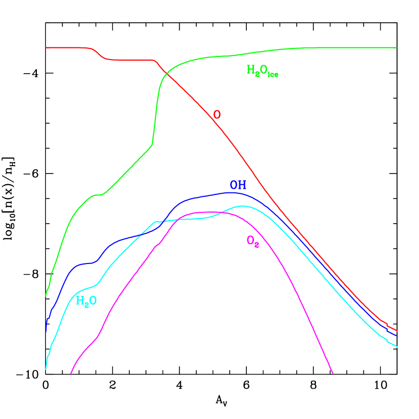
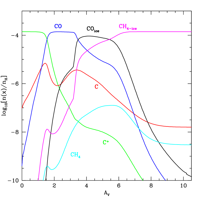
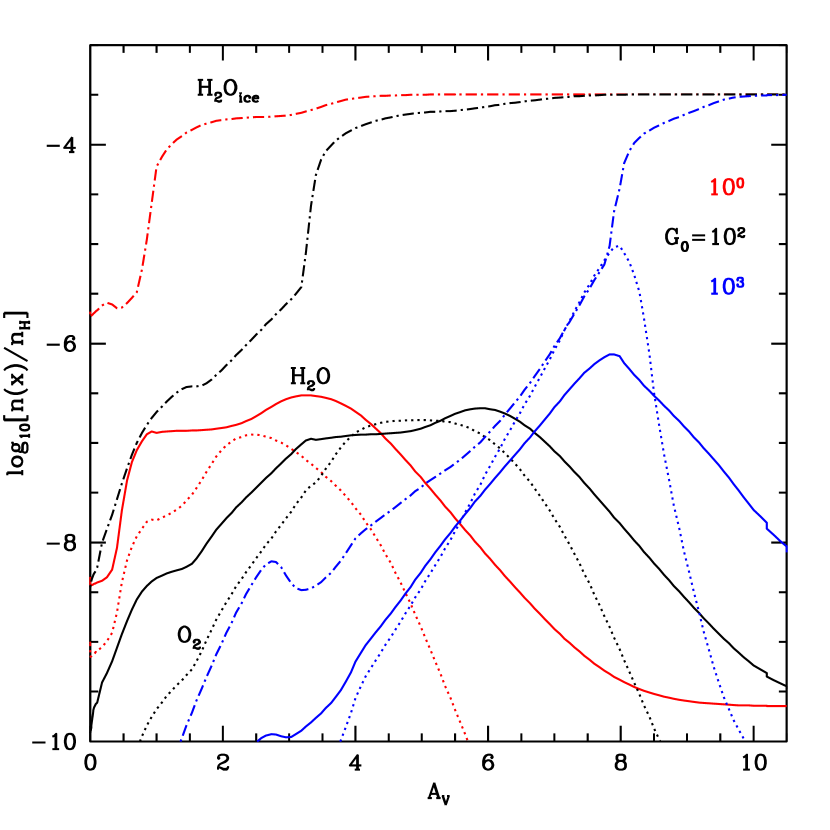
In the standard case, the gas (grain) temperature varies from $T=120$ K ($T_{gr}=31$ K) at the surface, to $T=22$ K ($T_{gr}=15$ K) at the water peak plateau, to $T=16$ K ($T_{gr}=15$ K) for $A_{V}=10$. The abundances of O-bearing species in the standard model are shown in Fig. 3, while those of C-bearing species are shown in Fig. 4. Here, the basic features of the results of freeze-out and desorption are clearly demonstrated.

The Photodissociation Layer. At the surface, the dominant species are precisely those found in gas-phase PDR models. Atomic oxygen is the most abundant O-bearing species, while the transition from C⁺ to CO occurs once significant shielding occurs at $A_{V}\sim 1.5$. Near the surface, all of the oxygen not in CO is atomic, and $x(O)\geq x(CO)$. At the low dust temperature at the surface, thermal desorption of H₂O is insignificant and the beginnings of an ice layer (less than a monolayer) form despite rapid photodesorption by the FUV. In steady-state, photodesorption of this ice as well as gas phase chemistry maintains a small abundance of gas-phase H₂O.

The Photodesorbed Layer. By $A_{V}\sim 2.8$, enough water has been deposited on grain surfaces to form a monolayer, that is $x({\rm H_{2}O_{ice})}\approx 4n_{gr}\sigma_{gr}N_{s,H_{2}O}/n\sim 8\times 10^{-6}(\sigma_{H}/2\times 10^{-21}$ cm²). At this point, the water ice abundance increases rapidly with depth. Here, the photodesorption rate decreases with depth due to attenuation of the FUV flux by grains, but the rate of freezeout only decreases when the gas phase O abundance decreases. For the gas phase O abundance to decrease significantly requires many monolayers of ice. This is seen in Fig. 3 as the increase in x(H₂O${}_{ice})$ by two orders of magnitude at $A_{V}\sim 3$. Note the agreement of this freezeout depth with $A_{Vf}$ given in Eq. (16). As the gas phase abundance of O decreases, the growth of water ice slows and the ice abundance saturates (i.e., all O nuclei locked in water ice) near $A_{V}\sim 3.5$. Fed by photodesorption, the gas phase abundance of H₂O maintains a broad plateau $x$(H₂O)$\sim 10^{-7}$ from $A_{V}\sim A_{Vf}\sim 3$ to $A_{V}\sim 6$, beyond which (i.e., deeper in the cloud) other gas phase H₂O destruction mechanisms besides photodissociation become dominant. The abundance of gas-phase H₂O near the peak is determined by the balance of photodesorption from the surface layer of ice on the grains with photodissociation of H₂O by FUV photons. Both of these processes are proportional to the local attenuated FUV field; this leads to a plateau in the H₂O abundance independent of $G_{0}$ (see §3.3).

The abundances of other O-bearing molecules closely track the abundance of H₂O. OH is mainly a product of photodissociation of gas-phase water, while it is destroyed by photodissociation and by reaction with S⁺, both of which depend on the attenuated FUV field. O₂ is produced primarily through the reaction O + OH $\rightarrow$ O₂ + H and is destroyed by photodissociation. Thus the gas-phase H₂O, OH and O₂ abundances track one another from the beginning of freezeout through the H₂O plateau. We discuss this in more detail in §3.3 below.

The Freezeout Layer. Beyond $A_{V}>6$, photodesorption of water ice ceases to produce enough gas phase H₂O or OH to maintain the H₂O and OH plateaus (and therefore the O₂ plateau). Other destruction mechanisms than photodissociation of H₂O take over, and gas phase abundances of all O-bearing species drop as H₂O ice incorporates essentially all available elemental O.

The destruction of CO by He⁺, followed by freezeout of the liberated O atom, as described in §2.3, is responsible for the rapid drop in the steady-state gas phase CO abundance at $A_{V}\sim 6$ (see Fig. 4) as all of the oxygen becomes locked in water ice. In our rather limited steady state carbon chemistry, C atoms end up incorporated into CH_4ice once O is liberated from CO. In our time-dependent runs, which have more extensive chemistry, the standard case at $A_{V}=10$ has $\sim 0.6$ of the elemental carbon in CH_4ice and $\sim 0.4$ in CO_ice after $2\times 10^{7}$ years. The ratio of the CH_4ice to the H₂O_ice abundance is $\sim 0.15-0.25$ at this time. Öberg et al (2008) discuss recent observational results on the ice content of grains in molecular clouds with emphasis on CH_4ice; they conclude that CH_4ice does indeed form by hydrogenation on grain surfaces, as we have assumed in our models. However, they observe abundance ratios of CH_4ice to H₂O_ice that are typically 0.05, nearly 3-5 times smaller than in our standard model. This likely arises because our time dependent code starts with carbon in atomic or singly ionized form, so that there is more opportunity for C or C⁺ to transform to CH_4ice than if the carbon started in the form of CO. Aikawa et al (2005) provide theoretical models that result in the observed ratios of CH_4ice/H₂O_ice by initiating carbon in the form of CO. The purpose of this paper is to follow H₂O and O₂ chemistry, and not carbon chemistry. We have therefore also neglected grain surface reactions that could lead to CO_2ice or methanol ice. Our CO_2ice is formed by first forming gas phase CO₂ by the reaction of gas phase CO with OH, and then subsequently freezing the CO₂ onto the grain surfaces. We plan to study the possible fractionation signature (¹²CO_2ice/¹³CO_2ice) of our gas phase route to forming CO_2ice in our subsequent paper which examines carbon chemistry in more detail (in preparation). In summary, our carbon chemistry here is simplified, and the abundances of carbon ices in the models are very crude.

3.2 Dependence on $G_{0}$, $n$, $Y_{H_{2}O}$, $\sigma_{H}$, PAHs, and $b_{\lambda}$

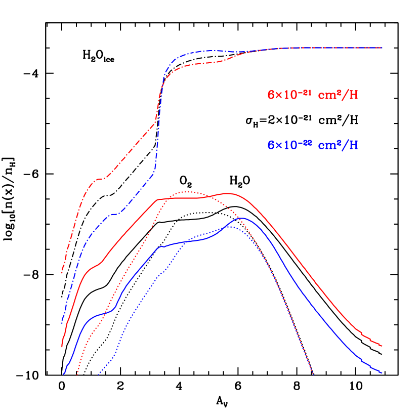
Dependence on Incident FUV Flux, $G_{0}$. Fig. 5 shows the effect of changing the FUV field strength, $G_{0}$, on the depth of the gas-phase water peak and the abundance at the peak, while keeping the density fixed. Here $G_{0}$ is varied from 1 to 10³. The main effect of changing $G_{0}$ is to move the position of the water peak inwards with increasing $G_{0}$. Varying $G_{0}$ from 1 to 10³ changes the depth of freezeout from $A_{V}\sim 1$ to $A_{V}\sim 7$. Gas phase H₂O peaks once ice has formed at least a monolayer on the grain surfaces, so the location of the water peak also moves inwards (logarithmically) with increasing $G_{0}$. The peak gas-phase water abundance ($\sim 10^{-7}$) is insensitive to $G_{0}$ and insensitive to depth (i.e., $A_{V}$) in the water plateau. We also see that the depth where the gas phase water starts to decline from its peak (plateau) value is also weakly (logarithmically) dependent on $G_{0}$, increasing with increasing $G_{0}$. Thus, the column of gas phase water remains fairly constant and independent of $G_{0}$.

However, some differences arise in the case with $G_{0}=10^{3}$. Here the assumption that every O sticking to a grain forms water ice breaks down. The high FUV field absorbed at the cloud surface leads to a high IR field that heats the grains to $T_{gr}\sim 25$ K even at $A_{V}\sim 8$, so that a significant fraction of O atoms are thermally desorbed from grains faster than they can form water ice, resulting in a higher gas phase abundance of atomic O. At these large depths, the formation of gas phase water is not mainly by photodesorption of water ice, but by cosmic ray initiated ion-molecule reactions (see Fig. 1). The high gas phase elemental abundance of O leads to a high rate of formation of H₂O and O₂, whereas the high $A_{V}$ leads to low photodestruction rates of these two molecules. In addition, although the FUV field is severely attenuated, the residual FUV is sufficient to prevent the complete freezeout of gas phase H₂O. The combined effect is a deeper and higher peak in the gas phase H₂O and O₂ abundances. At very high $A_{V}$ ($A_{V}>8$) the freezeout of water ice finally drains the gas phase oxygen, and gas phase H₂O and O₂ decrease with increasing $A_{V}$. Our time dependent results at $t=2\times 10^{7}$ years find most of the oxygen in H₂O-ice ($\sim 70$%) and CO₂-ice ($\sim 30$%) at $A_{V}>8$, and the carbon is mostly in C₃H-ice ($\sim 60$%) and CO₂-ice ($\sim 40$%) since the warm grain temperatures lead to thermal desorption of CO-ice and CH₄-ice.

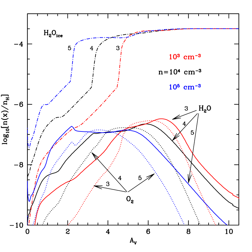
Dependence on Gas Density, $n$. In Fig. 6 we vary the gas density from $10^{3}$ to $10^{5}\,\rm cm^{-3}$, keeping the rest of the parameters fixed at their standard values. Comparing this figure with Fig. 5 we see that for $G_{0}<10^{3}$ the plateau water abundance is independent of gas density and $G_{0}$, depending only on the photoelectric yield $Y_{H_{2}O}$ and the grain cross sectional area per H nucleus $\sigma_{H}$ as shown below. The peak abundance is independent of $n$ because both the formation rate per unit volume (photodesorption) and the destruction rate (photodissociation) are proportional to $n$. For a fixed value of $G_{0}$, lowering the gas density moves the water peak further in; the deposition of water ice depends on the product $n_{gr}n_{O}\propto n^{2}$, while the photodesorption rate goes only as the grain density $n_{gr}\propto n$ times the local FUV field. Therefore, the water peak moves into the cloud with decreasing density. However, the column or $A_{V}$ where the water starts to decline from its peak (plateau) value is insensitive to $n$. Thus, the plateau starts to become narrower and narrower (in $\Delta A_{V}$) as $n$ decreases. As a result, The column of gas phase water increases with $n$ somewhat. We explain all these trends in more detail below in §3.3, where we present a simple analytic analysis.

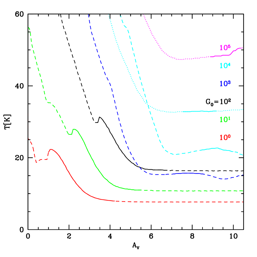
Dependence of Gas Temperature on $G_{0}$ and $n$. Figure 7 presents the gas temperature as a function of $A_{V}$ for a range of our $G_{0}$, $n$ parameter space. This figure reveals the temperature at which most of the H₂O and O₂ is radiating, as we have marked the peak in the gas phase water abundance (which coincides with the peak in the O₂ abundance) as solid portions of these curves. We see that over the parameter space $G_{0}=1-10^{5}$ the emission from H₂O and O₂ arises from regions of $T\sim 7-50$ K, with $T$ generally rising gradually with $G_{0}$. For $G_{0}<500$, there is a true “water plateau” and the solid line corresponds to the plateau region. $T\sim 7-30$ K in the plateau, and the gas temperature is often higher than the dust temperature because of grain photoelectric heating of the gas. For higher $G_{0}$ there is no true plateau but the gas phase H₂O and O₂ peak at higher $A_{V}$, where the gas and dust temperatures are nearly the same. We will show in §3.4 that at high $A_{V}$ the dust temperature scales roughly as $G_{0}^{0.24}$. Here we have made solid lines where the H₂O abundance is more than 0.33 of the peak abundance.

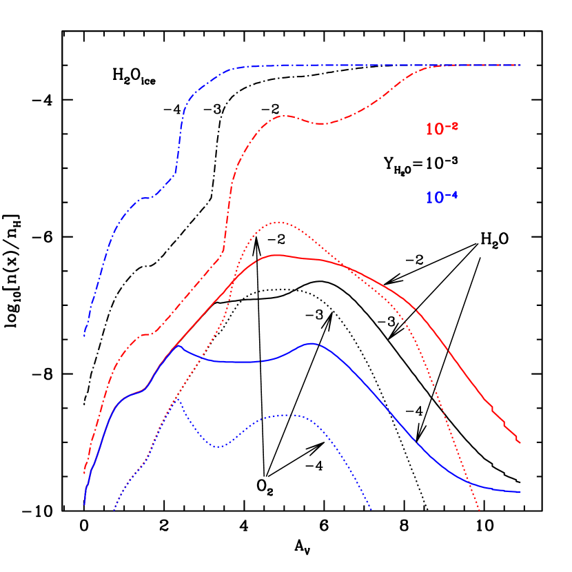
Dependence on Photodesorption Yield, $Y_{H_{2}O}$. Fig. 8 presents the profiles of the gas phase H₂O and O₂ abundances, and the H₂O ice abundance as the photodesorption yield $Y_{H_{2}O}$ of water ice is varied, maintaining $Y_{OH,w}=2Y_{H_{2}O}$, but keeping all other parameters standard. In contrast to the lack of dependence of the plateau value of the gas phase water abundance $x_{pl}(H_{2}O)$ on $n$ and $G_{0}$, $x_{pl}(H_{2}O)$ scales roughly linearly with $Y_{H_{2}O}$ for low $Y_{H_{2}O}<10^{-3}$. This linear dependence can be easily understood: the formation rate (photodesorption) of gas phase H₂O scales linearly with $Y_{H_{2}O}$ whereas the destruction rate (photodissociation) at a given $A_{V}$ is independent of $Y_{H_{2}O}$. On the other hand, at low values of $Y_{H_{2}O}<10^{-3}$, the abundance of O₂ rises with $Y_{H_{2}O}^{2}$, or, in other words, with [$x(H_{2}O)$]².

Dependence on Effective Grain Area, $\sigma_{H}$. In Figure 9 we show the effect of varying $\sigma_{H}$ with all other parameters at their standard values. The abundance of gas phase H₂O in the plateau $x_{pl}(H_{2}O)$ increases nearly linearly with $\sigma_{H}$. The depth $A_{V}\sim A_{Vf}$ where the H₂O abundance first reaches its plateau value is insensitive to $\sigma_{H}$, as predicted by Eq. (17). Similarly, the depth where H₂O finally begins to drop from its plateau value also is insensitive to $\sigma_{H}$. The abundance of O₂, like the abundance of H₂O, scales with $\sigma_{H}$.

Dependence on PAHs. We are most interested in the chemistry at $A_{V}\sim 3-6$ where the H₂O and O₂ abundances peak. Because it is not clear if PAHs exist at such depths (Boulanger et al 1990, Bernard et al 1993, Ristorcelli et al 2003), we have not included PAHs in our standard case but have assumed a grain surface area per H given by $\sigma_{H}$ which is appropriate to an MRN distribution extending down to 20 Å grains when computing the neutralization of the gas by collisions with small dust particles. If PAHs are present, the effect of neutralization is enhanced, which changes the gas phase chemistry somewhat. We have found that the inclusion of PAHs into our standard case does not affect the results appreciably. There is a somewhat greater effect at lower density such as $n\sim 100$ cm^-3, where the inclusion of PAHs does increase the total water column to high $A_{V}$ by a factor of about 10, both by broadening the peak plateau and by increasing the peak abundance (for the case $G_{0}=1$).

Dependence on $b_{\lambda}$. We have run our standard case but have assumed that the small grains responsible for FUV extinction are depleted, for example, by coagulation. In our test run we have decreased all our $b_{\lambda}$ by a factor of 2, reduced $\sigma_{H}$ by 2, and reduced grain photoelectric heating accordingly. The main effect is to increase the characteristic $A_{V}$ where the H₂O and O₂ plateau by a factor of 2. However, the abundances of H₂O and O₂ in the plateau decrease because of the decrease in $\sigma_{H}$. Therefore, the columns of gas phase H₂O and O₂ only increase by a factor of about 1.5 from the standard case. The gas temperature does not appreciably change. In summary, the change in the intensities and average abundances of $H_{2}$O and O₂ is not large, and is expected to be less than a factor of 2.

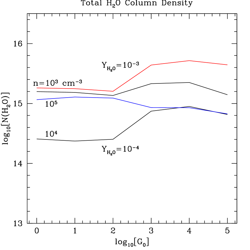
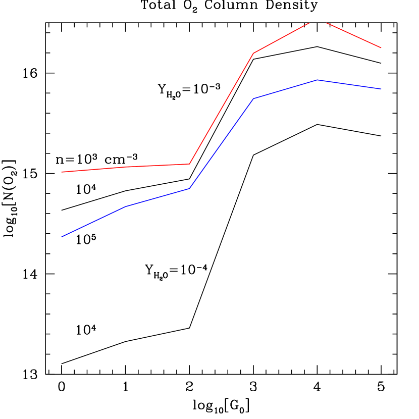
Dependence of H₂O and O₂ Columns on $G_{0}$ and $n$. In Fig. 10, we show the total columns of H₂O and O₂ for a cloud with high $A_{V}>10$ as a function of the incident FUV flux $G_{0}$ and the cloud density $n$. For low $G_{0}<500$, the H₂O and O₂ columns are roughly independent of $G_{0}$ and $n$, and are of order $10^{15}$ cm^-2 for our standard values of photodesorption yield. These columns arise in the H₂O and O₂ plateaus, at intermediate cloud columns. In the steady state models, there is so little gas phase water in the interior of the cloud that the interior does not contribute significantly to the total column. Therefore, once the total column through the cloud $N$ is large enough to include the plateau ($N_{H}\,\raise 1.29167pt\hbox{$>$}\kern-7.5pt\lower 3.01385pt\hbox{$\sim$}\,10^{22}$ cm^-2), the average abundance will scale as N_H^-1. Thus, part of the reason for the low average abundances observed by SWAS and Odin is the dilution caused by the lack of H₂O and O₂ at the surface and deep in the interior of very opaque, high column, clouds. At higher $G_{0}>500$ we see the effect of the thermal evaporation of the O atoms from the grain surfaces. The effect is most dramatic for the gas phase O₂ column, which rises to values $N(O_{2})\sim 2\times 10^{16}$ cm^-2. This is close to what is needed for a detection by Herschel and therefore it is in this type of environment that Herschel may potentially detect O₂. We note, however, that this result depends on the binding energy of O atoms to water ice surfaces. The value we have adopted (see Table 1) is standard in the literature but it refers to van der Waal binding to a chemically saturated surface. It is quite possible that the O binding energy is larger, and this would then increase the temperature (and $G_{0}$) where this effect would be initiated.

3.3 Simple Analytic Analysis of the Results

The results in §3.1 and §3.2 can be understood by a simple analytic chemical model that incorporates the main physics. Such a model, though approximate, has the advantage of allowing one to determine and understand the sensitivity to various model parameters, and serves to validate the numerical model. In this subsection the chemical rates are all taken from the UMIST database, except for the ion dipole rates and the photodesorption rates discussed in §2.7. In the following, the reader is referred to Table 3 in the Appendix for quick reference to symbols.

The abundance $x(H_{2}O)$ of gas phase H₂O can be roughly traced and understood by simple analytic formulae. Photodissociation dominates the destruction of gas phase H₂O from the surface to the depth $A_{Vd}$ where gas phase destruction with H${}_{3}^{+}$ generally takes over. From $0<A_{V}<A_{Vd}$ the simple model assumes that H₂O is formed by photodesorption of H₂O ice. Therefore, by equating formation to destruction

$$G_{0}F_{0}e^{-1.8A_{V}}Y_{H_{2}O}f_{s,H_{2}O}n_{gr}\sigma_{gr}=G_{0}R_{H_{2}O}e^{-1.7A_{V}}n(H_{2}O),$$ (19)

or

$$x(H_{2}O)=F_{0}Y_{H_{2}O}f_{s,H_{2}O}\sigma_{H}R_{H_{2}O}^{-1}e^{-0.1A_{V}},$$ (20)

where $R_{H_{2}O}=5.9\times 10^{-10}$ s^-1 is the unshielded photodissociation rate of H₂O in an FUV field of $G_{0}=1$. The differences in the $b_{\lambda}$ factors of 1.7 and 1.8 is because the two processes are dominated by somewhat different FUV wavelengths. The fractional coverage of the surface by water ice $f_{s,H_{2}O}$ is given by equating the sticking of O atoms to grain surfaces to the photodesorption rate of H₂O (including both desorption of H₂O and of OH + H). Therefore, recalling that $Y=Y_{H_{2}O}+Y_{OH,w}$,

$$n(O)v_{O}n_{gr}\sigma_{gr}=G_{0}F_{0}e^{-1.8A_{V}}Yf_{s,H_{2}O}n_{gr}\sigma_{gr}$$ (21)

or

$$f_{s,H_{2}O}={{n(O)v_{O}e^{1.8A_{V}}}\over{G_{0}F_{0}Y}}$$ (22)

Once a monolayer forms, $f_{s,H_{2}O}\sim 1$. We have found in our numerical runs that sometimes $f_{s,H_{2}O}$ saturates at $\sim 0.5$ rather than 1.0, because of the presence of other ices such as CO ice or CH₄ ice. However, assuming a saturation value of unity, the critical depth $A_{Vf}$ at which a monolayer forms is then given (this is equivalent to Eq. 17 in §2.5):

$$A_{Vf}=0.56\ln\left({{G_{0}F_{0}Y}\over{n(O)v_{O}}}\right),$$ (23)

or a critical H nucleus column (Spitzer 1978) from the surface of

$$N_{f}=2\times 10^{21}A_{Vf}\ {\rm cm}^{-2}.$$ (24)

We therefore find, using equations (20 and 22),

$$x(H_{2}O)={{n(O)v_{O}Y_{H_{2}O}\sigma_{H}e^{1.7A_{V}}}\over{YG_{0}R_{H_{2}O}}}\ \ {\rm for}\ A_{V}<A_{Vf}.$$ (25)

$$x_{pl}(H_{2}O)={{F_{0}Y_{H_{2}O}\sigma_{H}e^{-0.1A_{V}}}\over{R_{H_{2}O}}}\simeq 2\times 10^{-7}\left({Y_{H_{2}O}\over{10^{-3}}}\right)\left({\sigma_{H}\over{2\times 10^{-21}\ \rm cm^{2}}}\right)e^{-0.1A_{V}}\ \ {\rm for}\ A_{Vf}<A_{V}<A_{Vd}.$$ (26)

The abundance of gas phase H₂O rises exponentially with depth (as $e^{1.7A_{V}}$) until a monolayer of water ice has formed on the grains. It then forms a plateau with value $x_{pl}(H_{2}O)$ that is independent of $G_{0}$ and $n$ and weakly dependent on $A_{V}$. The plateau abundance goes linearly with $Y$ and $\sigma_{H}$. The lack of dependence on $G_{0}$ can be understood since both the formation and destruction of gas phase H₂O depend linearly on $G_{0}$. Higher fluxes do decrease the surface abundance of gas phase water, but the freezeout depth is deeper, so there is more dust attenuation, and the gas phase water abundance rises and peaks at the same constant value. More precisely, regardless of the incident FUV flux, the local attenuated FUV flux at the freezeout point is always the same, because it must be the flux which photodesorbs an ice covered grain at the rate that oxygen from the gas resupplies the surface with ice. Therefore, the gas phase water abundance is the same as well, regardless of $G_{0}$, only depending on the the assumed values of the grain parameters and the photodesorption yield. The lack of dependence on $n$ can be understood similarly since both the formation rate per unit volume and the destruction rate per unit volume depend linearly on $n$. On the other hand, $x(H_{2}O)\propto Y\sigma_{H}$, since the formation rate by photodesorption goes as this product whereas the destruction rate is independent of them.

In order to determine $A_{Vd}$ and to provide an approximation for $x(H_{2}O)$ that applies for $A_{V}>A_{Vd}$, we need to include other destruction routes for gas phase H₂O that begin to dominate at high $A_{V}$. We find that generally the route which takes over from photodissociation is reaction with H${}_{3}^{+}$ to form H₃O⁺. H₃O⁺ recombines one fourth of the time to reform water (not a net destruction) and three fourths of the time to form OH (Jensen et al 2000, Neufeld et al 2002). The net rate coefficient for the destruction of gas phase H₂O by H${}_{3}^{+}$ is then

$$\gamma_{H_{3}^{+}}=0.75(4.5\times 10^{-9}T_{300}^{-1/2})\ {\rm cm^{3}\ s^{-1}}.$$ (27)

where $T_{300}=T/300$ K. Equating the formation of gas phase H₂O by photodesorption to the destruction of H₂O by both photodissociation and H${}_{3}^{+}$, we obtain a more general solution for $x(H_{2}O)$ for $A_{V}>A_{Vf}$ that applies beyond $A_{Vd}$

$$x(H_{2}O)\simeq{{x_{pl}(H_{2}O)}\over{1+\left[{{\gamma_{H_{3}^{+}}n(H_{3}^{+})}\over{G_{0}R_{H_{2}O}}}\right]e^{1.7A_{V}}}}\ {\rm for}\ A_{V}>A_{Vf}.$$ (28)

Note that the second term in the denominator, which represents destruction by H${}_{3}^{+}$, begins to dominate when its value reaches and exceeds unity. At this point, $x(H_{2}O)$ begins to drop from its plateau value.

H${}_{3}^{+}$ is formed by cosmic rays ionizing H₂ followed by rapid reaction of H${}_{2}^{+}$ with H₂. When gas phase CO is depleted, it is destroyed by dissociative recombination with electrons. The electrons are provided by Si⁺ and S⁺ at moderate $A_{V}$ and by H${}_{3}^{+}$, He⁺, and H⁺ at high $A_{V}$, so the electron density is complicated. At high $A_{V}$ the code results suggest that the electron density is roughly $n(e)\simeq 2n(H_{3}^{+})$. We then obtain

$$n(H_{3}^{+})_{highA_{V}}\simeq 10^{-5}T_{300}^{1/4}n^{1/2}\ {\rm cm^{-3}},$$ (29)

with H nucleus density $n$ in cm^-3. In Eq. (29) we have assumed a total (including secondary ionizations) cosmic ray ionization rate of 5$\times 10^{-17}$ s^-1 for H₂ (Dalgarno 2006). At moderate $A_{V}$ Si⁺ usually provides most of the electrons. Gas phase Si⁺ is produced by photoionization of gas phase Si and destroyed by recombination with electrons. The Si⁺ density, and therefore the electrons provided by Si⁺, exponentially drops with $A_{V}$ as the FUV photons that photoionize Si drop with increasing dust attenuation. As long as most of the gas phase silicon is Si⁺, the electron density is high and this suppresses the abundance of H${}_{3}^{+}$, prolonging the water plateau to higher $A_{V}$ (see Eq. 28). However, we find that once the gas phase Si⁺ density drops to $2n(H_{3}^{+})_{highA_{V}}$, so that the electrons provided by Si⁺ are comparable to those provided by H${}_{3}^{+}$, He⁺, and H⁺, $n(H_{3}^{+})$ has risen to $\sim n(H_{3}^{+})_{highA_{V}}$ and the H${}_{3}^{+}$ term in the denominator of Eq. (28) dominates. Here the gas phase water abundance starts to fall. This occurs when

$$A_{Vd}=0.59\ln\left[4.5\times 10^{5}G_{0}n^{-1/2}T_{300}^{-0.2}\left({n_{SiT}\over n_{H_{2}O-gr}}\right)^{1/2}\right],$$ (30)

where $n_{SiT}=1.7\times 10^{-6}n$ is the density of silicon both in the gas phase and as ice mantles on grains, and $n_{H_{2}O-gr}\sim 3\times 10^{-4}n$ is the density of water molecules incorporated in ice mantles.

We have checked our analytic expressions for $A_{Vf}$ (Eq. 23), $A_{Vd}$ (Eq. 30), and $x_{pl}(H_{2}O)$ (Eq. 26) and find good agreement ($A_{Vf}$ and $A_{Vd}$ better than $\pm 25\%$ and $x_{pl}(H_{2}O)$ good to a factor of 2 over our ($G_{0}$,$n$) parameter space for $G_{0}\,\raise 1.29167pt\hbox{$<$}\kern-7.5pt\lower 3.01385pt\hbox{$\sim$}\,500$). For $G_{0}>500$ the grains are so warm that O atoms adsorbed to grains thermally evaporate before reacting with H atoms to form OH on the grain surface. As discussed in §3.2, this results in a change in the behaviour of gas phase H₂O.

The abundance of O, OH, and O₂ in the H₂O plateau region $A_{Vf}<A_{V}<A_{Vd}$ can also be analytically estimated from the above expression for $x_{pl}(H_{2}O)$. We first find $x_{pl}(OH)$ by equating formation by photodissociation of H₂O and photodesorption of OH from water ice with destruction by photodissociation of OH and reaction with S⁺ and He⁺. The photodesorption rate of OH is 2 times the rate of H₂O photodesorption, and therefore 2 times the rate of H₂O photodissociation. On the other hand, the destruction of OH by S⁺ and He$+$ is roughly 2 times that OH photodissociation. Therefore,

$$x_{pl}(OH)\sim\left({{R_{H_{2}O}}\over{R_{OH}}}\right)x_{pl}(H_{2}O)\sim 1.7x_{pl}(H_{2}O),\ \ A_{Vf}<A_{V}<A_{Vd}$$ (31)

where $R_{OH}=3.5\times 10^{-10}$ s^-1 is the unshielded photodissociation rate of OH when $G_{0}=1$. Thus, OH tracks H₂O with somewhat greater abundance in the plateau, as observed in Figure 3.

The gas phase O abundance is determined by balancing the formation of O by photodissociation of OH with the removal of O by adsorption onto grains:

$$x_{pl}(O)\simeq\left[{{G_{0}R_{OH}e^{-1.7A_{V}}}\over{\sigma_{H}nv_{O}}}\right]x_{pl}(OH)\simeq 4\times 10^{-5}\left({{G_{0}/n}\over 10^{-2}}\right)\left({e^{-1.7A_{V}}\over 10^{-3}}\right)\left({x_{pl}(H_{2}O)\over 10^{-7}}\right).$$ (32)

Therefore, $x_{pl}(O)$ exponentially declines with $e^{-1.7A_{V}}$ due to the declining photodissociation of OH, but the constant (with $A_{V}$) collision rate of O with grains, as seen in Figure 3. It also increases with $G_{0}/n$ for fixed $A_{V}$. This formula breaks down when the RHS exceeds $\sim 10^{-4}$, where $x_{pl}(O)$ saturates since all elemental gas phase O is now in atomic form.

The O₂ abundance follows from the abundances of O and OH since O₂ is formed by the neutral reaction of OH with O (rate coefficient $\gamma_{O_{2}}=4.3\times 10^{-11}(300\ {\rm K}/T)^{1/2}e^{-30\ {\rm K}/T}$ cm³ s^-1). O₂, like H₂O and OH, is destroyed by photodissociation in the plateau region. Therefore,

$$x_{pl}(O_{2}) \simeq \left[{{1.7^{2}\gamma_{O_{2}}}\over{\sigma_{H}v_{O}}}\right]\left({R_{OH}\over R_{O_{2}}}\right)e^{0.1A_{V}}[x_{pl}(H_{2}O)]^{2}$$

$$\sim 1\times 10^{-7}e^{0.1A_{V}}\left({{2\times 10^{-21}\ {\rm cm^{2}}}\over{\sigma_{H}}}\right)\left({30\over{T}}\right)e^{-30/T}\left[{x_{pl}(H_{2}O)\over 10^{-7}}\right]^{2},$$

where $R_{O_{2}}=6.9\times 10^{-10}$ s^-1 is the unshielded rate of photodissociation of O₂ in a $G_{0}=1$ field. The $[x_{pl}(H_{2}O)]^{2}$ dependence, which translates to a $Y_{H_{2}O}^{2}$ dependence in the plateau for low $Y_{H_{2}O}<10^{-3}$, is clearly seen in Figure 8. Note also that Eq. (33) explains the lack of dependence of $x_{pl}(O_{2})$ on $n$ and $G_{0}$, and also predicts that $x_{pl}(O_{2})\propto\sigma_{H}$ as observed in the numerical models.

In summary of the above, the approximate analytic equations can be used in the cases with $G_{0}\,\raise 1.29167pt\hbox{$<$}\kern-7.5pt\lower 3.01385pt\hbox{$\sim$}\,500$ to understand and quantitatively estimate: (i) $x_{pl}(H_{2}O,OH,O\ {\rm and}\ O_{2})$ and their dependence (or independence) on $n$, $G_{0}$, $Y$, and $\sigma_{H}$; (ii) the depth $A_{Vf}$ of the onset of the plateau, the depth $A_{Vd}$ of the termination of the plateau, the width $\Delta A_{V}=A_{Vd}-A_{Vf}$ of the plateau, and their dependence on the above parameters. At high $Y_{H_{2}O}>10^{-3}$ the abundances of O, OH, O₂, and H₂O are overestimated by factors of order 2 in the above formulae because we have ignored the presence of other ices, which reduce the fractional surface coverage of water ice, and therefore the production of gas phase H₂O and its photodissociation products.

Finally, the above analytic expressions can be used to predict the optimum conditions for observing H₂O and O₂. In general, for our model runs the intensity of the H₂O ground state ortho line at 557 GHz and para line at 1113 GHz can be estimated by assuming that the emission is “effectively thin”. In other words, although the optical depth in the ground state may be larger than unity, the gas density is so far below the critical density ($\sim 10^{8}$ cm^-3) that self absorbed photons are re-emitted and eventually escape the cloud (see discussion in §5). In this limit every collisional excitation results in an escaping photon, and

$$I_{557}\simeq{{h\nu[x_{o}n\gamma_{ex,o}+x_{p}n\gamma_{ex,p}]N(o-H_{2}O)}\over{4\pi}},$$ (34)

where $\gamma_{ex,o}\simeq 2.5\times 10^{-10}e^{-26.7/T}$ and $\gamma_{ex,p}\simeq 3.5\times 10^{-11}e^{-26.7/T}$ cm³ s^-1 (valid for $T\,\raise 1.29167pt\hbox{$<$}\kern-7.5pt\lower 3.01385pt\hbox{$\sim$}\,30$ K) are the rate coefficients for the collisional excitation of the 557 GHz transition by impact with ortho and para H₂ respectively (Faure et al 2007; M-L Dubernet, private communication). Here, $x_{o}$($x_{p}$) is the abundance of ortho(para)-H₂ with respect to H nuclei, $h\nu$ is the energy of the 557 GHz photon, and $N(o-H_{2}O)$ is the column of ortho water. Similarly, the para H₂O 1113 GHz line intensity is

$$I_{1113}\simeq{{h\nu[x_{o}n\gamma_{ex,o}+x_{p}n\gamma_{ex,p}]N(p-H_{2}O)}\over{4\pi}},$$ (35)

where where $\gamma_{ex,o}\simeq 3\times 10^{-10}e^{-53.4/T}$ and $\gamma_{ex,p}\simeq 9.0\times 10^{-11}e^{-53.4/T}$ cm³ s^-1 (valid for $T\,\raise 1.29167pt\hbox{$<$}\kern-7.5pt\lower 3.01385pt\hbox{$\sim$}\,30$ K) are the rate coefficients for the collisional excitation of the 1113 GHz transition by impact with ortho and para H₂. From the above equations, assuming most of the H₂O column arises in the plateau between $A_{Vf}$ and $A_{Vd}$, the ortho(para) H₂O column is given

$$N(o(p)-H_{2}O)\simeq 2\times 10^{21}(A_{Vd}-A_{Vf})x_{pl}(H_{2}O)f_{o}(f_{p})\ {\rm cm^{-2}},$$ (36)

where $f_{o}$($f_{p}$) is the fraction of H₂O in the ortho(para) state. Substituting our analytic equations for these parameters, we obtain

$$I_{557}\simeq 3\times 10^{-7}f_{o}[x_{o}+0.14x_{p}]\left({n\over{10^{4}\ \rm cm^{-3}}}\right)\left({Y_{H_{2}O}\over{10^{-3}}}\right)\left({\sigma_{H}\over{2\times 10^{-21}\rm cm^{2}}}\right)\Delta A_{V}e^{-0.1A_{V}}e^{-26.7/T}\ {\rm erg\ cm^{-2}\ s^{-1}\ sr^{-1}}$$ (37)

and

$$I_{1113}\simeq 2.4\left({f_{p}\over f_{o}}\right)\left({{x_{o}+0.3x_{p}}\over{x_{o}+0.14x_{p}}}\right)e^{-26.7/T}I_{557},$$ (38)

where $\Delta A_{V}=A_{Vd}-A_{vf}$. Note that the column of H₂O is relatively independent of $G_{0}$ and $n$. However, the intensity $I_{557}$ or $I_{1113}$ is proportional to the H₂O column times $\gamma_{ex}n\propto ne^{-26.7/T}$ or $ne^{-53.4/T}$, and therefore is somewhat sensitive to $G_{0}$ (which determines $T$) but is more sensitive to $n$. The 557 GHz line depends on $f_{o}$ which is a sensitive function of $T_{gr}$ for low $G_{0}$ (i.e., low $T_{gr}$), as will be described below. Therefore, the 557 or 1113 GHz H₂O line will be strongest in dense regions illuminated by strong FUV fluxes (assuming sufficient column or $A_{V}$ to encompass the plateau, and assuming the regions fill the beam). We note that the gas and grain temperatures vary somewhat through the water plateau region. We take the gas $T$ and the grain $T_{gr}$ to be the average of the values at the freezeout point $A_{Vf}$ and at the $A_{V}$ where the gas phase water abundance peaks. Figure 11 shows a contour plot of this average gas temperature $T_{ave}$ as a function of $G_{0}$ and $n$. Over nearly the entire range of $G_{0}$ and $n$, $T_{ave}$ only varies from $\sim 15-40$ K. Recall that Eqs (37) and (38) break down for $G_{0}\,\raise 1.29167pt\hbox{$>$}\kern-7.5pt\lower 3.01385pt\hbox{$\sim$}\,500$, but note that from our numerical results $I_{557}$ and $I_{1113}$ will increase further, and the analytic equations will underestimate the intensities with increasing $G_{0}$ above $G_{0}\sim 500$, since the water column rises here.

Similarly, we can estimate the intensity of the O₂ transition. Here, the density is above the critical density ($\sim 10^{3}$ cm^-3) for the 487 GHz O₂ transition so the levels are in LTE. In addition, because the transition has a low Einstein $A$ value, large columns are needed to make the transition optically thick. Thus, again assuming optically thin emission, the intensity $I_{487}\propto N(O_{2})e^{-25K/T}/Z(T)$, where $Z(T)$ is the partition function. An approximation to Z(T) for 0 K$<T<25$ K is given as $Z(T)\simeq 3+2.1T+0.1T^{2}$. Using the equations from this subsection, we then estimate

$$I_{487}\simeq 6\times 10^{-8}\left({{\Delta A_{V}}\over{Z(T)}}\right)\left({{30\ \rm K}\over T}\right)\left({Y_{H_{2}O}\over{10^{-3}}}\right)^{2}\left({\sigma_{H}\over{2\times 10^{-21}\rm cm^{2}}}\right)e^{-55/T}e^{-0.05(A_{Vf}+A_{Vd})}\ \ {\rm erg\ cm^{-2}\ s^{-1}\ sr^{-1}}$$ (39)

Note that again, this equation breaks down for $G_{0}\,\raise 1.29167pt\hbox{$>$}\kern-7.5pt\lower 3.01385pt\hbox{$\sim$}\,500$, and the equation will underestimate the intensity for higher $G_{0}$ since the O₂ column rises. In general, however, the equation predicts little $n$ dependence (there is a small $n$ dependence in the $A_{V}$ terms). At low $G_{0}\,\raise 1.29167pt\hbox{$<$}\kern-7.5pt\lower 3.01385pt\hbox{$\sim$}\,500$, the equation predicts only moderate $G_{0}$ dependence. Although various terms depend on $T$, the temperature of the O₂ plateau region is not sensitive to $G_{0}$ since the plateau retreats further into the shielded region for higher $G_{0}$. In addition, the $T$ dependence in the exp(-55/T) term is partially cancelled by the $TZ(T)$ term in the denominator.

3.4 The H₂O 557 and 1113 GHz and O₂ 487 GHz Line Intensities

Using the numerical models, Figures 12 and 13 present H₂O $I_{557}$ and $I_{1113}$ and O₂ $I_{487}$ contours as functions of $n$ and $G_{0}$ for fixed standard values of the other parameters. We have assumed that the H₂O ortho to para ratios are in LTE with the grain temperature (which in the plateau is nearly the same as the gas temperature except for very low ratios of $G_{0}/n$, which bring the plateau very close to the surface of the cloud where $T>T_{gr}$). The grain temperature is appropriate since a given H₂O molecule forms on a grain and spends too little time in the gas to equilibrate to the gas temperature before it is photodissociated. The grain temperature in the plateau is approximately (Hollenbach et al 1991)

$$T_{gr,pl}\simeq(3\times 10^{4}+2\times 10^{3}G_{0}^{1.2})^{0.2}.$$ (40)

A fit to the LTE ortho to para ratio of H₂O valid to 10% in the region 5 K $<T_{gr}<20$ K and good to 20% for $T_{gr}>20$ K (e.g. Mumma et al 1987) is given:

$${f_{o}\over f_{p}}=0.8e^{-{{22\,{\rm K}}\over T_{gr}}}+2.2e^{-\left({{15\,{\rm K}}\over T_{gr}}\right)^{2}}.$$ (41)

The H₂ ortho to para ratio is calculated in steady state using the rates and processes described by Burton et al (1992). They are neither 3 nor LTE. They are insensitive to $n$ in the plateau, but sensitive to $G_{0}$, which affects $T$. The H₂ ortho to para ratio $x_{o}/x_{p}\simeq 0.5$ at $G_{0}=3\times 10^{4}$, $0.3$ at $G_{0}=1.5\times 10^{4}$, and 0.1 for $G_{0}=4\times 10^{3}$. For lower values of $G_{0}$, $x_{o}/x_{p}<0.1$ so that para H₂ collisions dominate the excitation of water.

The 557 GHz and 1113 GHz intensities behave as described by the analytic formulae (Eq. 37 and 38) presented in §3.3 for $G_{0}\,\raise 1.29167pt\hbox{$<$}\kern-7.5pt\lower 3.01385pt\hbox{$\sim$}\,500$. The H₂O intensities rise roughly linearly with $n$. For fixed density $I_{557}$ and $I_{1113}$ tend to rise with $G_{0}$ (which raises $T_{gr}$ as shown in Eq.(40) and which tends to raise $T$ as can be seen in Fig. 11) partly due the excitation factors $e^{-26.7/T}$ and $e^{-53.4/T}$, but also because increasing $T$ increases the ortho/para ratio of H₂, and the ortho excitation rates in collisions with H₂O are much higher. $I_{1113}$ does not rise as much with increasing $G_{0}$ as one might naively expect given its excitation factor $e^{-53.4/T}$, because the increasing $T$ reduces $f_{p}$ from a value of $\sim 1$ at low $G_{0}$ to 0.25 at high $G_{0}$.

The following summarizes the accuracy of the analytic approximations for the H₂O and O₂ intensities for $Y_{H_{2}O}\sim 10^{-3}$. For $G_{0}<500$ the analytic expression for $I_{557}$ agrees with the numerical results to within a factor of 3 for $n=10^{3}-10^{5}$ cm^-3. The agreement for $I_{1113}$ is within a factor of 3 for $n=10^{4}-10^{5}$ cm^-3, but only to a factor of 5 (with the analytic underpredicting the intensity) for $n=10^{3}$ cm^-3. However, for this low value of $n$, the intensities are weak and not detectable. For higher values of $G_{0}$ the analytic formula underpredicts the intensity because of the larger columns of H₂O and O₂ (see Figure 10 and discussion). For higher values of $n$ the water plateau is so close to the surface that the gas temperature drops rapidly and significantly from $A_{Vf}$ to $A_{Vd}$; here the analytic formula is not accurate since it assumes constant average temperatures for both grains and gas. Nevertheless, the analytic formulae are useful in making estimates of line intensities, and also illustrate the dependences of the intensities on the physical parameters.

3.5 Model of Chemical Desorption

Following O’Neill, Viti, & Williams (2002), as discussed in §2.4, we have run our standard case with the modification that all molecules formed on grain surfaces instantly desorb. In our standard case only H₂ instantly desorbs. The basic differences are that the freezeout depth $A_{Vf}$ moves inward (increases) by about 2 magnitudes of visual extinction due to the chemical release of adsorbed OH and H₂O, the peak gas phase abundance of H₂O increases by about a factor of 10, and that of O₂ by a factor of roughly 100. We do not pursue this type of model further here, but note that it could warrant further study, although it appears to predict excessive H₂O and O₂ intensities. In the original O’Neill et al work, photodesorption and cosmic ray desorption were not included.

3.6 Model with No Grain Chemistry

In order to test the importance of the formation of OH, H₂O and carbon molecules on grain surfaces in our model, we have run the standard case ($G_{0}=100$, $n=10^{4}$) and two other cases ($G_{0}=100$, $n=10^{3}$ cm^-3 and $G_{0}=10$, $n=10^{4}$ cm^-3) with only H₂ formed on grain surfaces and no other grain chemistry. Like the model described above in §3.5, one main effect is to push the peak in the H₂O and O₂ abundances to higher $A_{V}$, since grain formation of H₂O is suppressed. However, in this case there is no enhancement of the peak abundances, because the formation rates of OH and H₂O are suppressed even more than in the case studied in §3.5. In addition, there can be significant depletion of gas phase elemental O at low $G_{0}$ by the formation of atomic O ice, which does not occur in §3.5 or in our models with grain chemistry in §3.1 and §3.2. In the ($G_{0}=100$, $n=10^{4}$ cm^-3) case and the ($G_{0}=10$, $n=10^{4}$ cm^-3) case, there is a reduction in both the columns of H₂O and O₂ and in the gas and grain temperatures of the emitting region compared to the cases with grain chemistry. Thus, the predicted lines are significantly weaker. Because of the good quality of our grain chemistry model fits to the data described in §4, and because of the laboratory and observational evidence for grain chemistry described in §2.3 and §3.1, we do not consider this case further.

3.7 Time Dependence

The numerical results and analytic solutions presented so far are for steady state solutions to the chemistry. However, as noted in §2.3 and §2.4, in the opaque interior of molecular clouds at $A_{V}>A_{Vd}$, the chemical timescales may exceed or be comparable to the cloud age, so that time dependent solutions to the chemistry are needed. The long chemical timescales include the freezeout of gas species onto grains for $n\,\raise 1.29167pt\hbox{$<$}\kern-7.5pt\lower 3.01385pt\hbox{$\sim$}\,10^{3}$ cm^-3 (see Eq. 1), the cosmic ray desorption of CO ice (see §2.4), and the conversion of gas phase CO to water ice which is initiated by He⁺ (see §2.3). In the opaque ”freezeout” regions the attenuated FUV flux plays little role in the chemistry so that the time dependent abundances do not vary with $A_{V}$. Therefore, we present results at a representative $A_{V}=10$ for the abundances of gas and ice species as a function of the age of the cloud, the density of the cloud, and the cosmic ray desorption rate of CO.

The time dependent code is that of Bergin et al (2000), updated to have the same grain chemistry and desorption processes as described above for the steady state code. It includes more species than the PDR surface code, and therefore tracks the carbon chemistry more accurately in the inner regions. It takes as initial conditions the chemistry of translucent clouds: all the hydrogen is initially molecular H₂ with the other species atomic (for ionization potentials $>13.6$ eV) or singly ionized otherwise.

The results are shown in Figures 14 and 15, where we present the abundances of O₂, H₂O and CO plotted as a function of the cosmic ray desorption rate of CO ice, for two times representative of cloud ages ($2\times 10^{6}$ years in Fig. 14 and $2\times 10^{7}$ years in Fig. 15), for the standard $G_{0}=100$, and for 3 densities ($10^{3}$, $10^{4}$, and $10^{5}$ cm^-3). Of particular note is Figure 15, where one sees the gas phase molecules increase in abundance as the cosmic ray desorption rate increases, reach a peak when the timescale for cosmic ray desorption of CO is about 0.1 - 1.0 times the cloud evolution time of 2$\times 10^{7}$ years, and then decreases as the cosmic ray rate increases further and the desorption time becomes less than $\sim 2\times 10^{6}$ years. If the rate is too low, then the CO ice remains on the grain and the gas phases abundances are low. If the rate is too high, then the CO ice rapidly desorbs, but then the CO in the gas breaks down by reaction with He⁺ and the gas phase elemental oxygen freezes out as water ice, thereby lowering the gas phase abundances of CO, H₂O, and O₂. The main point is that in all cases for $t=2\times 10^{7}$ years and for most cases with $t=2\times 10^{6}$ years, the abundances of H₂O and O₂ at high $A_{V}$, even when time dependent chemistry is taken into account (steady state chemistry is more extreme in this respect as seen in Figure 3), are substantially lower than the peak abundances of these molecules at intermediate $A_{V}$. Thus, most of the column of these molecules in molecular clouds are not provided by the interior regions, where they are frozen out, nor by the surface, where they are photodissociated. Rather, most of the column arises from the intermediate zone.

3.8 Chemistry: the Gas Phase C/O Ratio

Figures 16 and 17 show the gas phase elemental abundance of C and the gas phase abundance ratio of elemental C/O, as a function of $A_{V}$, for two different cloud ages, $t=2\times 10^{6}$ years and $t=2\times 10^{7}$ years, respectively. In each figure, we plot the standard case, the standard case but with the density changed to $n=10^{3}$ and $10^{5}$ cm^-3, and the standard case but with the incident FUV field changed to $G_{0}=1$ and $10^{3}$. For these results, we have used our time dependent models, since the interesting effect of C/O exceeding unity occurs at high $A_{V}$, where the time dependent models are more relevant and are more accurate in treating the carbon chemistry. At early times, $t\sim 2\times 10^{6}$ years, the C/O ratio generally stays below unity at high $A_{V}$. The exception is the high density ($n=10^{5}$ cm^-3) case, but here the gas phase elemental abundance of carbon is extremely low, which implies low abundances of any organic molecules produced in this carbon-rich environment. At late times, $t\sim 2\times 10^{7}$ years, we see that all cases except the high $G_{0}=10^{3}$ case result in gas phase C/O$>1$ for $A_{V}\,\raise 1.29167pt\hbox{$>$}\kern-7.5pt\lower 3.01385pt\hbox{$\sim$}\,8$, due to the preferential freezeout of water ice which robs the gas of elemental O. For those cases with C/O$>1$, the gas phase elemental C abundance increases with increasing $G_{0}$ and decreasing $n$, due to increased thermal desorption rates of carbon molecular ices and decreased freezeout rates, respectively. Figure 17 shows that for densities $n\sim 10^{3}-10^{4}$ cm^-3 and $G_{0}=1-100$, strong chemical effects might be observed deep in clouds, with high abundances of gas phase hydrocarbons and other carbon molecules rather than CO. Unfortunately, these results can only be viewed as suggestive, because the gas phase C depends on the desorption rate of CO, CH₄ and other carbon species frozen to grain surfaces, and these are uncertain. Nevertheless, it appears that regions with C/O $>1$ and high gas phase elemental C abundance can appear deep in the cloud. This is consistent with the chemistry of GMC cores such as Orion A (e.g., Bergin et al 1997) and regions in the Taurus Molecular Cloud (e.g., Pratap et al 1997). In addition, in these deep layers significant amounts of CH₄ ice may form, and its release to the gas stimulates the carbon chemistry. In summary, the freezeout of the oxygen into water ice can have profound effects on the carbon chemistry deep in the cloud and the ability of the cloud to produce carbon chain molecules or hydrocarbons.

3.9 Limb Brightening and Surface to Volume Effects

Because our model suggests a peak in the H₂O and O₂ abundance at intermediate depths into a molecular cloud, one might expect clouds to be limb-brightened if viewed with beams smaller than the cloud. We make here two caveats to this prediction. First, GMCs are clumpy, and the clumpiness means that $A_{Vf}$ will occur at different physical depths (i.e., radii) in the clouds, depending on the particular radial ray through the cloud and where it intersects clumps. This will have the effect of smearing the limb-brightening. In addition, although the 557 and 1113 GHz H₂O transitions are ”effectively thin”, they do suffer numerous scattering events since the optical depth in the lines are greater than unity. This scattering will reduce the limb-brightening effect for the H₂O transitions. The O₂ does not suffer scattering, so it may be more promising. However, the sensitivity of Herschel may require large O₂ columns $>10^{16}$ cm^-2, and these may only be achieved for high $G_{0}$. In such cases, the peak O₂ abundance occurs deep in the cloud, $A_{V}\sim 8$, and makes limb brightening only possible to detect in very high column but extended nearby clouds illuminated by high fields. Nevertheless, Herschel observations of O₂ in clouds may find regions of limb-brightening.

One still would like to map the clouds, however, even if limb brightening is hard to detect. The regions of high $G_{0}$ may be fairly limited in spatial extent, and our models predict higher H₂O and especially O₂ columns in these regions which Herschel may spatially resolve. In addition, the H₂O and O₂ plateaus extend for $\Delta A_{V}\sim 3$. For gas densities of $n\sim 10^{4}$ cm^-3 this corresponds to $\sim 0.2$ pc, which at 500 pc corresponds to an angular size $\sim 1.5^{\prime}$. Therefore, for a PDR slab viewed edge-on, Herschel may resolve the plateau region.

Even for clouds too small in angular extent to map, our model can be tested by correlation studies of the H₂O and O₂ intensities with the intensities of rotational transitions of other molecules known to trace either the surface or the volume of the cloud. For example, ¹³CO and C¹⁸O are thought to generally trace the volume of the cloud, whereas PDR species such as CN trace the ”surface” of the cloud (Fuente et al 1995, Rodriguez-Franco et al 1998). We are investigating such observational correlations in Melnick et al (in preparation).

4 APPLICATIONS TO SPECIFIC SOURCES

4.1 Diffuse Clouds

The diffuse clouds that we model, based on those observed by SWAS towards W51 and W49 where H₂O 557 GHz is seen in absorption, are characterized by $G_{0}\sim 1-10$, $n\sim 100$ cm^-3, and $A_{V}\sim 1-5$ [these are sometimes called “translucent clouds” (Snow & McCall, 2006)]. Diffuse clouds are illuminated on all sides by the diffuse interstellar FUV field, whereas our models are those of 1D slabs illuminated from one side. To roughly construct a model of a diffuse cloud of total thickness $A_{Vt}$, we take the results from $A_{V}=0$ to 0.5$A_{Vt}$ and assume a mirror image for the rest of the cloud from 0.5$A_{Vt}$ to $A_{Vt}$.

We compare a single model fit of a diffuse cloud with the 54 and 68 km s^-1 velocity components observed by SWAS towards the background submillimeter source W49 (Plume et al., 2004) as well as in the single absorption component towards W51 (Neufeld et al., 2002) . For all three of these components, both OH and H₂O column densities have been measured, with N(H₂O)$\sim 1-3\times 10^{13}\,\rm cm^{-2}$ and N(OH)/N(H₂O) $\sim$ 3-4. Our diffuse cloud model with $n=10^{2}\,\rm cm^{-3}$ and $G_{0}=1$ gives N(H₂O)=$3\times 10^{13}\,\rm cm^{-2}$ and N(OH)/N(H₂O) =3.5 for a total cloud extinction of $A_{Vt}$= 4.4 magnitudes. We find that assuming a photodesorption yield $Y_{OH,w}\simeq 2\times Y_{H_{2}O}$ provides the best fit to the observed N(OH)/N(H₂O) ratios. The same model also provides predicted ¹²CO and atomic C columns and line intensities of the ¹²CO J=1-0, J=3-2 and [CI] 609 $\mu$m lines, all of which were observed in the W49 components. The models overpredict the columns and the intensities of the CO J=1-0 and [CI] lines by a factor $\sim 3$ which may be explained by dilution of the emission lines in the beam. The J=3-2 line, however, is predicted to be a factor $\sim 2$ smaller than is observed; a better fit for this line is found at higher densities, but makes the fit of all the other observed lines poorer. We note that Bensch et al (2003) had similar problems in fitting a PDR model to the diffuse cloud CO and [CI] results.

Comparing our H₂O column to the model $A_{Vt}$, we find a column-avearged H₂O abundance of $3\times 10^{-9}$ with respect to H nuclei. The observational papers cited above quote H₂O/H₂ abundance ratios $>10^{-7}$. These high abundances, however, were derived from the observed CO columns by multiplying the CO columns by $10^{4}$ to obtain H₂ columns. In our models, we find H₂ columns of $\sim 4\times 10^{21}$ cm^-2 and H₂O/H₂ abundance ratios of $\sim 10^{-8}$. The H₂/CO column-averaged abundance ratio in the model is $1.3\times 10^{5}$. In these translucent clouds, CO is photodissociated much more than H$2$, which self-shields much more effectively. Considerable H₂ exists in regions where the gas phase carbons is mostly C⁺. These translucent clouds are examples of ”dark H₂” which is not traced by CO.

4.2 Dense, Opaque Clouds

4.2.1 A_V Thresholds for Ice Formation

Whittet et al (2001) have presented plots of the water ice columns versus cloud extinction in which a clear threshold $A_{V}$ for water ice is inferred. In our model we identify that threshold $A_{V}$ with $A_{Vf}$, since the ice very rapidly builds up with increasing $A_{V}$ once the grain has a monolayer of ice. Whittet et al (2001), Tanaka et al (1990), and Williams, Hartquist & Whittet (1992) find that $A_{Vf}\sim 3$ for Taurus and $\sim 6$ for $\rho$ Oph. Assuming the radiation field in Taurus is $G_{0}\sim 1$ and that the gas density is $10^{3}$ cm^-3, we predict from our analytic model with $Y=3\times 10^{-3}$ (i.e., $Y_{H_{2}O}=10^{-3}$, recall that $Y$ is the total yield of both H₂O and of OH+H being ejected from water ice) that $A_{Vf}=3$. For $\rho$ Oph, Liseau et al. (1999) and Kamegai et al (2003) have estimated $G_{0}\sim 100-1000$ as an average value in the SWAS beam. Assuming $n=10^{3}-10^{4}$ cm^-3 in the ambient gas averaged over the beam, we predict $A_{Vf}\simeq 6$. Thus, our model does a good job of matching these thresholds. Note that the threshold $A_{Vf}$ in our model mainly depends on $\ln(G_{0}Y/n)$ and so to the extent that we know $G_{0}/n$, we can constrain $Y$. We therefore see that $Y\sim 3\times 10^{-3}$ is a reasonable choice for interstellar ice grains..

4.2.2 B68

B68 is one of the best-studied, nearby, isolated molecular clouds (Alves et al. 2001, Zucconi et al. 2001). It lies at $\sim 160$ pc, with a mean density of $\overline{n}\sim 10^{5}$ cm^-3, an $A_{V}$ through the cloud center of $\sim 30$, and a central temperature of 7 K. Extinction and dust continuum maps have recently provided a detailed view of the density and temperature structure of the cloud (Alves et al. 2001, Zucconi et al. 2001). Previous models of the CO lines and the exterior temperature of the cloud suggest $G_{0}\sim 0.25-1$ (Bergin et al., 2002). The angular size of the cloud is $\sim 1.3\arcmin$, smaller than the SWAS beamsize.

SWAS has performed long integrations on B68 searching for the 557 GHz H₂O line and the 487 GHz O₂ line, setting stringent 3$\sigma$ upper limits on the line strengths (assuming thermal linewidths) from these undetected transitions of $I_{557}\,\raise 1.29167pt\hbox{$<$}\kern-7.5pt\lower 3.01385pt\hbox{$\sim$}\,4\times 10^{-9}$ erg cm^-2 s^-1 sr^-1 and $I_{487}\,\raise 1.29167pt\hbox{$<$}\kern-7.5pt\lower 3.01385pt\hbox{$\sim$}\,6\times 10^{-9}$ erg cm^-2 s^-1 sr^-1. Utilizing the known distribution of density $n$ with $A_{V}$, and assuming $G_{0}=0.5$ and our standard values of $Y$ and $\sigma_{H}$, we have modeled the H₂O and O₂ abundance profiles and the expected observed line strengths in B68. To compare with the observed intensities, we calculate the intensity expected in the model and then dilute the intensity by the cloud area divided by the SWAS beam area. Averaged over the SWAS beam, the predicted line intensities of $I_{557}\sim 4\times 10^{-11}$ erg cm^-2 s^-1 sr^-1 and $I_{487}\sim 1\times 10^{-12}$ erg cm^-2 s^-1 sr^-1 lie well below the upper limits set by SWAS. We predict a non-beam-diluted line intensity $I_{1113}\sim 10^{-8}$ erg cm^-2 s^-1 sr^-1, which is not detectable by Herschel. Because the 557 GHz and 487 GHz line intensities are sensitive to $G_{0}$ (via the gas and dust temperatures), regions like B68 with low FUV fields are not promising targets for H₂O and O₂ detections.

Another interesting effect in our modeling of B68 arises because our models incorporate the observed increase of density with depth $A_{V}$. From Figure 6 one sees that this reduces the width $\Delta A_{V}$ of the H₂O plateau since the lower density surface gas means that $A_{Vf}$ is larger, whereas the higher density gas in the interior makes $A_{Vd}$ smaller. However, this effect is not large, since our B68 model has $n=1.3\times 10^{5}$ cm^-3 at $A_{V}=1$, $n=1.7\times 10^{5}$ cm^-3 at $A_{V}=2$, and $n=2.4\times 10^{5}$ cm^-3 at $A_{V}=3$ (roughly the extent of the H₂O plateau). We find that our predicted column of H₂O in our density-varying model differs by only 10% from a constant density, $n=1.7\times 10^{5}$ cm^-3, model.

4.2.3 NGC2024

NGC2024 is a dense, $n\sim 10^{5}$ cm^-3 star forming molecular cloud in Orion illuminated by a relatively intense, $G_{0}\sim 10^{4}$, FUV field (Gianini et al., 2000). Contrasted to B68, it provides a test of our models for elevated radiation fields (i.e., $G_{0}>500$). SWAS has observed both the H₂O 557 GHz line and the O₂ 487 GHz line in this source. We have reanalyzed the SWAS data from the archives and obtain a beam-averaged intensity of $3\times 10^{-7}$ erg cm^-2 s^-1 sr^-1 for the 557 GHz line and a 3 sigma upper limit on the 487 GHz line of $4\times 10^{-8}$ erg cm^-2 s^-1 sr^-1 [see also Snell et al (2000) for the 557 GHz line and Goldsmith et al (2000) for the 487 GHz upper limit].

Our models (see Figs. 12 and 13) reproduce the H₂O 557 GHz line with beam averaged gas densities $n\sim 10^{4.8}$ cm^-3 and $G_{0}\sim 10^{4}$, assuming that the ortho/para H₂O ratio is in LTE with the grain temperature and the ortho/para ratio of H₂ is the steady state value from the formulation by Burton et al (1992). Here, in our peak water plateau, the gas temperature is $\sim$27 K, and the ortho/para ratio of H₂ is $\sim 1/6$. The grain temperature is $\sim 42$ K and the ortho/para ratio of H₂O is 2.7. In the model the O₂ 487 GHz line intensity is predicted to be $4\times 10^{-9}$ erg cm^-2 s^-1 sr^-1, well below SWAS detectability. The peak (plateau) abundances for H₂O and O₂ in the model are (see Figs. 5 and 6) $10^{-7}$ and $3\times 10^{-6}$ respectively. The column averaged abundances, assuming $N\sim 4\times 10^{22}$ cm^-2 or $A_{V}\sim 20$ through the cloud (Gianini et al., 2000, based on CO column densities greater than few$\times 10^{18}$ cm^-2 over a $\sim 4\arcmin$ region) is $\overline{x}(H_{2}O)\equiv N(H_{2}O)/N\simeq 1.1\times 10^{-8}$, and $\overline{x}(O_{2})\simeq 1.7\times 10^{-7}$. We conclude that the models also provide good fits to NGC2024, using reasonable values of $n$ and $G_{0}$, and predict peak abundances that are approximately 10 times greater than the column averaged abundances. We predict $I_{1113}\sim 3\times 10^{-7}$ erg cm^-2 s^-1 sr^-1, which is detectable by the HIFI instrument on the Herschel Observatory.

4.2.4 O₂ Observed by Odin in $\rho$ Oph

Larsson et al (2007) have reported the detection of the ground state transition of O₂ at 119 GHz with the space submillimeter telescope Odin. Note that this is a different transition than the O₂ transition observed by SWAS, and is at a much longer wavelength. Therefore, although the Odin telescope has twice the diameter of SWAS, the Odin beam size at 119 GHz ($\sim 10^{\prime}$) is more than twice that of the SWAS beam at 487 GHz. At the distance of $\rho$ Oph, the Odin beam corresponds to 0.4 pc. The beam was centered on a 450 $\mu$m peak, and the submillimeter dust emission and the CO isotopic rotational emission suggest an H₂ column of $2\times 10^{22}$ cm^-2 ($A_{V}\sim 20$). A temperature of 30 K has been obtained for both the gas (e.g., Loren et al 1990) and the dust (Ristorcelli et al, in preparation) in this region. Using these parameters, and assuming the O₂ to be optically thin and in LTE, Larsson et al find a column $N(O_{2})\sim 1\times 10^{15}$ cm^-2 for an abundance relative to H₂ of $\sim 5\times 10^{-8}$ but an abundance in our units (relative to H nuclei) of $x(O_{2})=2.5\times 10^{-8}$. The authors acknowledge a possible uncertainty of at least a factor of 2 in their estimate of the O₂ abundance.

The $\rho$ Oph region observed is illuminated on the back side by a B2 V star, with the cool dense cloud core sitting in front of the photodissociation region. The relatively high dust temperature, and the likely distance of the B star from the cloud, suggest $G_{0}\sim 100-1000$ shining on the cloud surface (Cesarsky et al., 1976; Kamegai et al., 2003). The 0.4 pc size coupled with the observed total H₂ column suggest $n\sim 10^{5}$ cm^-3 in this dense region. Setting $G_{0}=300$ and $n=10^{5}$ cm^-3, and using standard parameters, we obtain a column $N(O_{2})=1.4\times 10^{15}$ cm^-2. In our model, the gas and dust temperatures at the O₂ abundance peak are $\sim 20$ K. We predict (see Figs. 12 and 13) an H₂O 557 GHz intensity of $I_{557}=10^{-7}$ erg cm^-2 s^-1 sr^-1, and a O₂ 487 GHz intensity of $I_{487}=2\times 10^{-9}$ erg cm^-2 s^-1 sr^-1 from this region. We have analyzed SWAS archival data on this source and find a measured H₂O 557 GHz intensity of $1.3\times 10^{-7}$ erg cm^-2 s^-1 sr^-1 and a 3$\sigma$ upper limit of $2\times 10^{-8}$ erg cm^-2 s^-1 sr^-1 for the O₂ 487 GHz line. We predict $I_{1113}\sim 3\times 10^{-7}$ erg cm^-2 s^-1 sr^-1, which may be marginally detectable by the HIFI instrument on Herschel. In summary, our model successfully fits the H₂O and O₂ observations of $\rho$ Oph, using reasonable parameters for this region.

4.2.5 Upper Limits on O₂ Observed by Odin

Pagani et al (2003) report 3$\sigma$ upper limits on $N(O_{2})$ in a number of sources. As examples of sources with low incident $G_{0}$, the upper limits for TMC1 and L183 (L134N) are $7\times 10^{14}$ and $1.1\times 10^{15}$ cm^-2, respectively. Although the Odin beam is large, these sources are extended enough that beam dilution should not be a significant factor. In addition, although much of the Taurus cloud has relatively low total $A_{V}$, these regions appear to have sufficiently high $A_{V}\,\raise 1.29167pt\hbox{$>$}\kern-7.5pt\lower 3.01385pt\hbox{$\sim$}\,10$ to encompass the O₂ plateau. Using an estimated $G_{0}\sim 1$ and $n\sim 10^{4}$ cm^-3, our models predict a column of $N(O_{2})\sim 4\times 10^{14}$ cm^-2 (see Figure 10) on both sides of the cloud, for a total column of $\sim 8\times 10^{14}$ cm^-2. This prediction lies very close to the observed upper limits. If future observations or analysis drive this upper limit down below our predicted value, then either beam dilution or a lower value of $Y_{H_{2}O}$ need to be invoked to reconcile observations with the models. Note that the upper limits on $N(O_{2})$ set upper limits on $Y_{H_{2}O}\,\raise 1.29167pt\hbox{$<$}\kern-7.5pt\lower 3.01385pt\hbox{$\sim$}\,10^{-3}$.

More challenging to our model are the upper limits quoted for sources with relatively high $G_{0}$. For example, Pagani et al report 3$\sigma$ upper limits of $N(O_{2})<1.9\times 10^{15}$ cm^-2 for Orion A. This column is averaged over the $9^{\prime}$ beam of Odin, which corresponds to a linear extent (diameter) of about 1.4 pc at the distance of Orion. If there were no extinction from the source of the FUV (primarily $\Theta^{1}C$ in the Trapezium), the FUV flux at a distance of 0.7 pc from the star corresponds to $G_{0}\sim 4\times 10^{3}$. Taking this as the average $G_{0}$ incident on the molecular cloud in the beam, our model predicts $N(O_{2})\sim 10^{16}$ cm^-2 (see Figure 10), significantly higher than the observed upper limit. We offer two possible explanations for this discrepancy. First, $\Theta^{1}C$ may be inside a cavity in the cloud carved out by the champagne flow created by the Trapezium. In this case, extinction by the intervening cloud would diminish $G_{0}$ in the outer regions of the beam, and thereby diminish the beam average column of O₂. A second possibility arises from the fact that the enhancement of the O₂ column at high $G_{0}$, as discussed in §3.2, is caused by the thermal evaporation of O atoms from grain surfaces before they can react to form water ice on the surface. We have adopted a binding energy of O atoms to the grain surface of $E_{O}/k=800$ K (see Table 1). However, this binding energy is uncertain and in our view may be low, given that O is a radical. A modest increase in this binding energy would result in a much higher critical $G_{0}$ where the enhancement of $N(O_{2})$ occurs, since the grain temperature is a weak function of $G_{0}$ ($T_{gr}\propto G_{0}^{0.2}$) and thus the critical $G_{0}$ goes as $E_{O}^{5}$. In other words, increasing $E_{O}/k$ to 1200 K would increase the critical $G_{0}$ from about 500 to about 4000, and provide a solution consistent with the observations.

Sandqvist et al (2008) use Odin observations to place an upper limit of $N(O_{2})<6\times 10^{16}$ cm^-2 toward SgrA. As noted in that paper, this is consistent with our model clouds for any incident $G_{0}$ and any density $n$ for standard local gas phase elemental abundances of O and C.

5 SUMMARY, DISCUSSION AND CONCLUSIONS

We have constructed both a detailed numerical code and simple analytical equations to follow the abundances of the main oxygen-bearing species as a function of depth in molecular clouds. We take clouds of constant density $n$, illuminated by an external FUV (6 eV$<h\nu<13.6$ eV) field characterized by the unitless parameter $G_{0}$ normalized to the local (Milky Way) interstellar FUV field. We explore the range 10³ cm${}^{-3}<n<10^{6}$ cm^-3 and $1<G_{0}<10^{5}$. Our models incorporate thermal balance, gas phase chemistry, a simple grain surface chemistry that includes the formation of H₂, H₂O, and CH₄ on grain surfaces, the sticking of gas phase species to grain surfaces, and various desorption processes such as photodesorption, thermal desorption, and cosmic ray desorption.

The abundances of chemical species vary considerably as a function of depth into a molecular cloud. At the surface, molecules are photodissociated and the gas is primarily atomic (e.g., O) or, for species with ionization potentials less than 13.6 eV, singly ionized (e.g., C⁺). Here, although dust grains may be cold enough to prevent rapid thermal desorption, ices do not form because photodesorption keeps the refractory dust clear of ice mantles (the same is true of dust in the diffuse ISM). Very deep in the cloud, again assuming grains cold enough to prevent thermal desorption, photodesorption is negligible and ices form, causing gas phase abundances of condensibles to plummet. Here, time dependent effects (generally associated with cosmic rays) dominate the gas phase chemistry due to the time required to deplete condensibles onto grains, to desorb CO ice by cosmic rays, and to destroy gas-phase CO (by He⁺ produced by cosmic rays). These processes are slow, and have timescales comparable to, or longer than, typical molecular cloud lifetimes. At intermediate depths, photodesorption of ices supply gas phase elements, and the partial shielding of the photodissociating external FUV flux allows gas phase molecular abundances to peak.

We have focused in this paper on oxygen chemistry, and followed in particular the gas phase species O, OH, O₂, and H₂O as well as water ice. Our answer to the longstanding astrochemical question, “Where is elemental O in molecular clouds?”, is that oxygen not in CO is primarily gas phase atomic O to a depth $A_{Vf}$ (see Eq. 23), and is water ice at larger depths. The freezeout depth $A_{Vf}$ where significant water ice forms is proportional to $\ln(G_{0}/n)$, and is typically 3-6. Refractory silicate grains contain a modest abundance of O ($\sim 10^{-4}$), but the bulk is likely gas phase O and CO along with CO ice and H₂O ice. For example, in our standard model, integrating to $A_{V}=10$, the O not in refractory grains is divided $56$% H₂O-ice, $25$% gas phase O, $10$% CO-ice, and $8$% gas phase CO.

Our models also give an indication of the origin of water in molecular clouds. In the steady state standard model, at $A_{Vf}$ the formation rate of gas phase H₂O is 2% via gas phase reactions and 98% by photodesorption of H₂O that has been formed on grains. At $A_{Vd}$ the percentages are 30% and 70%, respectively; midway in the plateau, they are 8% and 92%, respectively. These percentages depend on $G_{0}$ and $n$, but as long as $G_{0}\,\raise 1.29167pt\hbox{$<$}\kern-7.5pt\lower 3.01385pt\hbox{$\sim$}\,500$, these numbers are representative. At higher $G_{0}>500$, where O atoms thermally desorb from grains before forming OH and eventually water ice, most of the water production is via gas phase reactions. The production of water ice is about 3 times greater than the production of gas phase water by photodesorption of water ice, because 2/3rds of the water ice is photodesorbed as OH. Thus, one needs to modify these numbers if one wants to estimate the formation of water in any form in a cloud: for example, in the standard case midway in the plateau the percentages are 3% by gas phase reactions and 97% by grain surface reactions.

We plan a follow-up paper to examine carbon chemistry. We note that Figure 14 shows that for all densities considered and by $t>2\times 10^{6}$ years, gas phase CO is largely absent in cloud interiors. This is in rough agreement with observations that show CO depletions in dense cloud interiors. Thus, CO is not always a volume tracer. However, the sequel paper will include more grain surface carbon chemistry such as the formation of CO₂ and methanol on grain surfaces. In addition, we will examine the effects of initial conditions on time-dependent chemistry, and compare observations with a wide variety of models with varying cosmic ray desorption rates and gas density profiles through the cloud.

For $G_{0}\,\raise 1.29167pt\hbox{$<$}\kern-7.5pt\lower 3.01385pt\hbox{$\sim$}\,500$, the abundances of gas phase OH, O₂ and H₂O peak and plateau at values $\sim 10^{-7}$ between $A_{vf}$ and $A_{Vd}$ (see, Eqs. 26, 31, and 33). These abundances are independent of $n$ and $G_{0}$ because both their formation rate (ultimately from photodesorption of H₂O ice) and their destruction rate (from photodissociation) both depend on the product $nG_{0}$. However, since their formation is linked with H₂O ice photodesorption, these plateau abundances do increase with increasing ice photodesorption yield, $Y_{H_{2}O}$ and $Y_{OH,w}$, and also with the grain cross sectional area per H nucleus $\sigma_{H}$ (see same equations).

For higher values of $G_{0}\gtrsim 500$, the chemistry undergoes a change, as O atoms no longer form H₂O ice on grain surfaces. Here, the grains are warm enough ($\,\raise 1.29167pt\hbox{$>$}\kern-7.5pt\lower 3.01385pt\hbox{$\sim$}\,20$ K) that O atoms thermally desorb before reacting with H atoms. This pushes the freezeout to greater depths and enhances the abundances of gas phase O, OH, O₂ and H₂O by keeping more of the elemental oxygen in the gas phase. Because O₂ formation goes as the product of O and OH abundances, O₂ is the most sensitive to this change and its local abundance reaches $10^{-5}$, while its column climbs to $\sim 2\times 10^{16}$ cm^-2. We note that the observations of Pagani et al (2003) may suggest a higher binding energy for O on grains than adopted, and in this case the critical $G_{0}$ where this occurs may be significantly higher than 500.

Deep in the cloud interior at $A_{V}>>A_{Vf}$, the gas phase abundances drop as ices become dominant, the exact values of the abundances depending on cloud lifetimes and the cosmic ray desorption rates assumed (see Figures 14 and 15). Here, time dependent chemistry dominates.

Poelman, Spaans, & Tielens (2007) have suggested that the SWAS results do not rule out substantial gas phase H₂O abundances and columns in the centers of clouds, because of optical depth effects which “hide” the H₂O in the centers. However, as this saturation effect occurs, the line center antenna temperature approaches the gas temperature of the emitting region. In our model, this gas temperature is typically 10-20 K. Even in the cold interior of clouds, one would expect temperatures of 5-10 K. The SWAS observed antenna temperatures in regions of detected H₂O are of order $T_{A}<1$ K. This result alone suggests the H₂O is in the “effectively optically thin” regime. Our model does include an escape probability formalism for the H₂O lines. We find, in agreement with Poelman et al, that significant collisional de-excitation and saturation of the line occurs when $\tau n/n_{cr}>1$, where $\tau$ is the line center optical depth and $n_{cr}$ is the critical density ($\sim 10^{8}$ cm^-3 for the 557 GHz line). Thus, the requirement for 557 GHz line saturation is roughly

$$\left[{N(H_{2}O)\over{6\times 10^{12}\ {\rm cm^{-2}}}}\right]{n\over n_{cr}}\,\raise 1.29167pt\hbox{$>$}\kern-7.5pt\lower 3.01385pt\hbox{$\sim$}\,1.$$ (42)

Since our models have $N(H_{2}O)\sim 10^{15}$ cm^-2 and $n\,\raise 1.29167pt\hbox{$<$}\kern-7.5pt\lower 3.01385pt\hbox{$\sim$}\,10^{6}$ cm^-3, we are almost always within the effectively optically thin regime, except perhaps for the highest densities $n\sim 10^{6}$ cm^-3. Furthermore, if the H₂O columns and densities were high enough that line saturation occurred, the line fluxes would exceed those observed by SWAS. We argue that SWAS observations indicate effectively thin 557 GHz emission, and that there is no evidence for hidden H₂O in the centers of clouds.

Bergin et al (2000) listed ingredients for a successful astrochemical model of a molecular cloud. Slightly updated, they included: (1) low column-averaged abundances ($\,\raise 1.29167pt\hbox{$<$}\kern-7.5pt\lower 3.01385pt\hbox{$\sim$}\,10^{-7}$) of gas phase O₂, (2) low column-averaged abundances ($\,\raise 1.29167pt\hbox{$<$}\kern-7.5pt\lower 3.01385pt\hbox{$\sim$}\,3\times 10^{-8}$) of gas phase H₂O, (3) an explanation of the apparently higher abundances of H₂O when it is observed in absorption in translucent clouds, (4) column-averaged water ice abundances of $\sim 10^{-4}$, and (5) existence of complex carbon-bearing species in the gas phase in some regions. As noted above, the model presented in this paper fulfills all of these criteria.

In addition, we have successfully applied, in a simple way, these models to observations of the $A_{V}$ threshold for the onset of water ice, the strict upper limits for the gas phase H₂O abundance in B68 made by SWAS, the possible detection of O₂ in $\rho$ Oph made by Odin, the detection of H₂O and upper limits for O₂ made by SWAS for NGC 2024, and upper limits of the O₂ abundance set by Odin.

These successes imply that the proper modeling of the interstellar chemistry of molecular clouds must include as ingredients: photodissociation, freezeout on grains, grain surface chemistry, desorption processes, and, in the very opaque central regions, time-dependent chemistry. At the surface photodissociation and photodesorption dominate. Deep in the cloud, dust vacuums the condensibles and slow cosmic ray processes are important, requiring time-dependent chemistry. At intermediate depths, gas phase molecular species such as O₂ and H₂O peak in abundance, and provide the source of their submillimeter emission.

Appendix A Appendix

Table 1: Adsorption Energies, Photodesorption Yields, and Cosmic-Ray Desorption Rates of Surface Monolayer Atoms and Molecules

Species	Adsorption Energy	Photodesorption Yield	Cosmic-Ray Desorption Rate
	[K]	[UV Photon]-1	[mol-1 s-1]
O	800	$10^{-4}$	—
OH	1300	$10^{-3}$	—
H2O	4800	$10^{-3}$ as H2O	$4.4\times 10^{-17}$
		$2\times 10^{-3}$ as OH
O2	1200	$10^{-3}$	$9.1\times 10^{-15}$
C	800	$10^{-3}$	—
CH	650	$10^{-3}$	—
CH2	960	$10^{-3}$	—
CH3	1200	$10^{-3}$	—
CH4	1100	$10^{-3}$	$2.7\times 10^{-15}$
CO	960	$10^{-3}$	$6.0\times 10^{-13}$
S	1100	$10^{-3}$	—
Si	2700	$10^{-3}$	—
Fe	4200	$10^{-3}$	—

Table 2: Standard Model Parameters

Parameter	Symbol	Value
H nucleus density	$n$	$10^{4}\,\rm cm^{-3}$
FUV field	$G_{0}$	100
Oxygen abundance	$x_{O}$	$3.2\times 10^{-4}$
Carbon abundance	$x_{C}$	$1.4\times 10^{-4}$
Sulfur abundance	$x_{S}$	$2.8\times 10^{-5}$
Silicon abundance	$x_{Si}$	$1.7\times 10^{-6}$
Magnesium abundance	$x_{Mg}$	$1.1\times 10^{-6}$
Iron abundance	$x_{Fe}$	$1.7\times 10^{-7}$
Total grain cross section per H nucleus	$\sigma_{H}$	$2\times 10^{-21}\,\rm cm^{2}$

Table 3: Symbols Used in the Text

Symbol	Definition
$a$	grain radius
$A_{V}$	visual extinction from surface of the cloud
$A_{Vf}$	visual extinction where there is onset of water ice freezeout, monolayer of ice forms
$A_{Vd}$	visual extinction where the gas phase water abundance drops
$\Delta A_{V}$	width of the plateau of gas phase H2O or O2, or $(A_{Vd}-A_{Vf})$
$E_{i}$	binding energy of species $i$ to grain surface
$f_{\rm o},(f_{\rm p})$	fraction of H2O in the ortho(para) state
$f_{s,i}$	fraction of surface sites occupied by species $i$
$F_{\rm FUV}$	flux of FUV photons at the cloud surface
$F_{0}$	$10^{8}$ photons cm-2 s-1, the flux of FUV photons corresponding to $G_{0}=1$
$F_{pd,i}$	flux of molecules of species $i$ photodesorbing from ice surface
$F_{td,i}$	flux of molecules of species $i$ thermally desorbing from ice surface
$G_{0}$	unitless parameter measuring incident FUV flux normalized to $1.6\times 10^{-3}$ erg cm-2 s-1
	or to $10^{8}$ photons cm-2 s-1, roughly the local interstellar value
$\gamma_{\rm He^{+}}$	net rate coefficient for destruction of H2O by He+
$\gamma_{\rm H_{3}^{+}}$	net rate coefficient for destruction of H2O by H${}_{3}^{+}$
$\gamma_{\rm O_{2}}$	rate coefficient for gas phase reaction of OH with O to form O2
$I_{487}$	intensity of the O2 487 GHz transition, in erg cm-2 s-1 sr-1
$I_{557}$	intensity of the H2O 557 GHz transition, in erg cm-2 s-1 sr-1
$I_{1113}$	intensity of the H2O 1113 GHz transition, in erg cm-2 s-1 sr-1
$n$	gas phase hydrogen nucleus number density [$\sim n({\rm H})+2n({\rm H_{2}}+n({\rm H^{+}})$]
$n_{gr}$	number density of grains
$\nu_{i}$	vibrational frequency of species $i$ bound to a grain surface
$N$	gas-phase column density of hydrogen nuclei
$N_{i}$	gas-phase column density of species $i$
$N_{f}$	column density of hydrogen nuclei for onset of water ice freezeout
$N_{s,i}$	number of adsorption sites per cm2 on a grain surface ($\simeq 10^{15}\,{\rm cm^{-2}}$)
$R_{td,i}$	thermal desorption rate of per atom or molecule of species $i$ from a surface
$R_{cr,i}$	cosmic ray desorption rate per surface atom or molecule, $i$
$R_{\rm H_{2}O}$	$5.9\times 10^{-10}$ s-1, the unshielded photodissociation rate per molecule of H2O for G0=1
$R_{\rm O_{2}}$	$6.9\times 10^{-10}$ s-1, the unshielded photodissociation rate per molecule of O2 for G0=1
$R_{\rm OH}$	$3.5\times 10^{-10}$ s-1, the unshielded photodissociation rate per molecule of OH for G0=1
$\sigma_{\rm H}$	grain cross sectional area per H nucleus
$\sigma_{gr}$	cross sectional area of a single grain
$t_{cr,i}$	timescale for cosmic ray desorption of adsorbed ice species $i$ with abundance $x(i)$
$t_{evap,{\rm H_{2}O}}$	time for an adsorbed H2O molecule to thermally evaporate from a grain surface
$t_{evap,{\rm O}}$	time for an adsorbed O atom to thermally evaporate from a grain surface
$t_{f,i}$	timescale for species $i$ to hit (and stick to) a grain
$t_{\gamma}$	timescale for a grain of size $a>100\,$Å  to absorb an FUV photon at the cloud surface
$t_{\gamma,f}$	timescale for a grain of size $a>100\,$Å  to absorb an FUV photon at $A_{V,f}$
$t_{\gamma-des}$	timescale to photodesorb an O atom from a grain with covering factor $f_{s,{\rm O}}$
$t_{gr,i}$	time for a given grain to be struck by a gas phase atom or molecule of species $i$
$t_{r}$	timescale for a grain to radiate much of its thermal energy
$T_{ave}$	the average of the gas $T$ at $A_{Vf}$ and at the $A_{V}$ where the H2O abundance peaks
$T_{max}$	peak temperature of a grain after absorbing one FUV photon
$T_{300}$	$T/300$ K, where $T$ is the gas temperature
$x(i)$	abundance of species $i$ relative to H nuclei
$x_{o}$	abundance of ortho-H2
$x_{p}$	abundance of para-H2
$x_{pl,i}$	abundance of species $i$ in the plateau region between $A_{Vf}$ and $A_{Vd}$
$Y_{i}$	photodesorption yield of species $i$ from a grain surface
$Y$	$Y_{\rm H_{2}O}+Y_{{\rm OH},w}$, the total yield of H2O and OH being desorbed from water ice surface
$Z({\rm T})$	partition function for O2

Figure 1: Standard ion-neutral chemistry leading to the formation of H₂O and O₂ in shielded regions of the ISM. The chemistry is often initiated by cosmic ray ionization of H₂. The resultant H${}_{2}^{+}$ reacts with H₂ to form H${}_{3}^{+}$. An alternate route starts with the cosmic ray ionization of hydrogen and the resultant change exchange of H⁺ with O to form O⁺.

Figure 2: Grain-surface oxygen chemical network included in this modeling effort. Note that in addition we include grain surface carbon chemistry (see text) and allow the sticking of all species onto grain surfaces and various desorption mechanisms. The grain surface oxygen reaction network begins with O sticking to grains, followed by accretion of H to form OH_ice and then H₂O_ice. Here, “$d$” stands for the three desorption processes: thermal, photo-, and cosmic ray. Near the cloud surface, FUV photons photodesorb ices, leading to some gas-phase H₂O and O₂. In addition, for high FUV fields which warm the grains, thermal desorption of the weakly bound O atoms can be important both near the surface and deep in the cloud. Finally, deep in the cloud, cosmic ray desorption is important.

Figure 3: Oxygen chemistry for the standard ($n=10^{4}$ cm^-3, $G_{0}=100$) steady-state PDR model, including freeze- out, grain-surface reactions, thermal desorption, photodesorption, and cosmic ray desorption. Model parameters are those given in Table 1. The abundances of major O-bearing species are shown as a function of visual extinction from the cloud surface, $A_{V}$.

Figure 4: Carbon chemistry for the standard ($n=10^{4}$ cm^-3, $G_{0}=100$) steady-state PDR model, including freeze- out, grain-surface reactions, thermal desorption, photodesorption and cosmic ray desorption. Model parameters are those given in Table 1. The abundances of major C-bearing species are shown as a function of visual extinction from the cloud surface, $A_{V}$. For $A_{V}>5$, the gas phase CO abundance wlll not be as low as is shown here for the steady-state solution; time-dependent effects will keep the CO abundance elevated (see §3.7). In addition, the limited chemistry in the steady state PDR code drives the high abundance of CH₄ ice at high $A_{V}$; the time dependent code, which has more extensive chemistry, finds a mixture of CO and CH₄ ice for the carbon-bearing ices in this case.

Figure 5: H₂O, O₂ and H₂O_ice abundances for a cloud with $n=10^{4}\,\rm cm^{-3}$ but with a variety of FUV field strengths incident on the cloud surface. Results are shown for FUV fields G₀=1, 10² and 10³ times the average interstellar field. H₂O_ice is dot-dash, H₂O is solid, and O₂ is dotted lines. Higher $G_{0}$ drives curves to the right. Although the depth at which freezeout occurs is affected by $G_{0}$, the total H₂O column is not. The increase in the peak abundance of O₂ seen for $G_{0}=1000$ is caused by thermal desorption of atomic O from the warm grains, which suppresses H₂O_ice formation and keeps more elemental O in the gas phase.

Figure 6: Effect of changing the gas density. Results are shown for $n=10^{3}$, $10^{4}$ and $10^{5}\,\rm cm^{-3}$ and for the standard FUV field $G_{0}=10^{2}$. The threshold $A_{V}$ for water ice formation and the $A_{V}$ where H₂O and O₂ peak increase for increasing $G_{0}/n$. The peak abundances do not change with $n$. The labels on the arrrows refer to the log of the density $n$.

Figure 7: The gas temperature $T$ as a function of $A_{V}$ for a variety of $n$ and $G_{0}$ with all other parameters standard. Dashed lines refer to gas density $n=10^{4}$ cm^-3, and in order of increasing $T$ at low $A_{V}$ correspond to $G_{0}=1$, 10, 100, 10³, and 10⁴. Dotted lines refer to gas density $n=10^{5}$ cm^-3, and in order of increasing $T$ correspond to $G_{0}=10^{4}$ and $10^{5}$ (Orion PDR conditions). The solid portion of each curve refers to the region of the “water plateau” for $G_{0}<500$, or to regions where the water abundance is at least 0.33 times its peak value for $G_{0}>500$.

Figure 8: Abundances of H₂O, H₂O_ice and O₂ for the standard case ($n=10^{4}$ cm^-3, $G_{0}=100$) as a function of $A_{V}$ and of the photodesorption yield of water ice to form gas-phase H₂O, $Y_{\rm H_{2}O}$. Results are shown for the standard yield of 10^-3 and for yields of 10^-2 and 10^-4. H₂O_ice also photodesorbs OH with a rate two times $Y_{\rm H_{2}O}$ (see text). The labels refer to the log of the yield.

Figure 9: Abundances of H₂O, O₂ and H₂O_ice as a function of $A_{V}$ and of the total grain cross section per H nucleus, $\sigma_{H}$. The higher curves for O₂ and H₂O and the lower curves for H₂O_ice refer to higher values of $\sigma_{H}$.

Figure 10: The total columns of H₂O (left panel) and O₂ (right panel) as a function of $G_{0}$ and $n$, assuming clouds with $A_{V}$ greater than the plateau values, or roughly $A_{V}\,\raise 1.29167pt\hbox{$>$}\kern-7.5pt\lower 3.01385pt\hbox{$\sim$}\,3-6$. The increase of the column of H₂O and O₂ at $G_{0}\sim 500$ is caused by the thermal desorption of O atoms from grain surfaces, which suppresses the formation of water ice and enhances the gas phase abundance of elemental O. Note that since the column is produced at intermediate $A_{V}$, the column average abundance of H₂O and O₂ will fall as $A_{V}^{-1}$ for high $A_{V}$. Results are shown for the standard photoyield $Y_{H_{2}O}=10^{-3}$ for densities of $10^{3}$, $10^{4}$, and $10^{5}$ cm^-3, and for $Y_{H_{2}O}=10^{-4}$ for a density of $10^{4}$ cm^-3.

Figure 11: The average (see text) gas temperature in the water plateau region or the peak water abundance region for a range of densities and FUV field strengths incident on the cloud surface. Note that the temperature only increases by a factor of $\sim 3$ while the incident FUV flux $G_{0}$ increases by $10^{5}$. The plateau retreats deeper into the cloud as $G_{0}$ increases, which suppresses a more dramatic increase in $T$.

Figure 12: H₂O intensities for a range of densities and FUV field strengths incident on the cloud surface. Contours are labeled with the logarithm of intensity, measured in units of ${\rm erg\ s^{-1}\ cm^{-2}\ sr^{-1}}$. Left Panel: Intensity of the ortho-H₂O groud state transition $1_{1,0}-1_{0,1}$ at 557 GHz. To convert to units of ${\rm K\,km\,s^{-1}}$, multiply contour levels by $5.6\times 10^{6}$; Right Panel: Intensities of the para-H₂O ground state transition $1_{1,1}-0_{0,0}$ at 1113 GHz. To convert to units of ${\rm K\,km\,s^{-1}}$, multiply contour levels by $7.0\times 10^{5}$.

Figure 13: The O₂ 487 GHz intensity for a variety of densities and FUV field strengths incident on the cloud surface. Contours are labeled with the logarithm of intensity, measured in units of ${\rm erg\ s^{-1}\ cm^{-2}\ sr^{-1}}$. To convert to units of ${\rm K\,km\,s^{-1}}$, multiply contour levels by $8.4\times 10^{6}$. Note the relative constancy of the O₂ intensity for $G_{0}<100$, since the column and temperature of the O₂ plateau region stay quite constant.

Figure 14: Abundances of H₂O (solid), CO (dot-dash) and O₂ (dotted) at A${}_{V}=10$ at a cloud age of $2\times 10^{6}$ years, for a range of CO cosmic-ray desorption rates. Our standard CO cosmic-ray rate is given by $k(CO_{cr})_{0}$ and is given in Table 1. Results are shown for rates from $10^{-2}$ to $10^{2}$ times the standard rate, for G${}_{0}=100$ and densities $n_{\rm H}=10^{3}$, $10^{4}$, and $10^{5}{\rm cm^{-3}}$. The higher densities have lower abundances due to freezeout of gas species. Note that the H₂O and O₂ abundances are only significant (i.e., comparable to the plateau value), for low densities. The timescale $t_{cr,CO}$ for cosmic ray desorption of CO ice (see Eq. 8) is given at the top.

Figure 15: Same as Fig. 14 but for an age of of $2\times 10^{7}$ years. Note that the H₂O and O₂ abundances are never significant compared to their plateau values. If the cosmic ray desorption timescale for CO ice, $t_{cr,CO}$ is long, the H₂O and O₂ abundances are low because the frozen CO is not liberated to the gas to provide elemental gas phase O to form them. If the timescale is very short, the CO ice is desorbed quickly and the gas has time to deplete the elemental gas phase O as water ice on the grain surfaces.

Figure 16: Ratio of carbon nuclei to oxygen nuclei in the gas phase for clouds with a variety of densities and FUV field strengths. Results are shown for a cloud age of 2$\times 10^{6}$ years. If the C/O ratio rises above unity, then interesting organic chemistry ensues (see text). Note that the C/O ratio only rises above unity for one case (the high density, $n=10^{5}$ cm^-3 case). However, in this case the time to deplete the gas phase carbon is very short so that the gas phase elemental C abundance is very low (bottom panel). Thus, the abundance of organic molecules will be very low.

Figure 17: Same as Figure 16 but for cloud age of 2$\times 10^{7}$ years. Note that C/O rises above unity for all cases except the case with high $G_{0}=10^{3}$. Thus, in all cases but this one, complex carbon chemistry is initiated, since not all C will be tied up in CO. The bottom panel shows which clouds will have the highest abundance of these molecules (the cases with C/O$>1$ and high elemental C abundance). The elemental C abundance rises with increasing $G_{0}/n$.

References

- Aikawa et al. (1996) Aikawa, Y., Miyama, S. M., Nakano, T., & Umebayashi, T. 1996, ApJ, 467, 684
- Aikawa et al. (2005) Aikawa, Y., Herbst, E., Roberts, H., & Caselli, P. 2005, ApJ, 620, 330
- Adams et al. (1985) Adams, N. G., Smith, D., & Clary, D. C. 1985, ApJ, 296, L31
- Alves et al. (2001) Alves, J.F., Lada, C.J., & Lada, E.A. 2001, Nature, 409, 159
- Andersson et al (2006) Andersson, S., Al-Halabi, A., Kroes, G-J., & van Dishoeck, E.F. 2006, J. Chem. Phys., 124, 4715
- Bensch et al. (2003) Bensch, F., Leuenhagen, U., Stutzki, J., & Schieder, R. 2003, ApJ, 591, 1013
- Bergin et al. (1997) Bergin, E. A., Goldsmith, P. F., Snell, R. L., & Langer, W. D. 1997, ApJ, 482, 285
- Bergin et al. (1998) Bergin, E. A., Neufeld, D. A., & Melnick, G. J. 1998, ApJ, 499, 777
- Bergin et al. (2000) Bergin, E. A., et al. 2000, ApJ, 539, L129
- Bergin et al. (2002) Bergin, E.A., Alves, J., Huard, T. & Lada, 2002, ApJ, 570, L101
- Bergin et al. (2003) Bergin, E. A., Kaufman, M. J., Melnick, G. J., Snell, R. L., & Howe, J. E. 2003, ApJ, 582, 830
- Bergin & Tafalla (2007) Bergin, E. A., & Tafalla, M. 2007, ARA&A, 45, 339
- Bernard et al. (1993) Bernard, J. P., Boulanger, F., & Puget, J. L. 1993, A&A, 277, 609
- Boulanger et al. (1990) Boulanger, F., Falgarone, E., Puget, J. L., & Helou, G. 1990, ApJ, 364, 136
- Bringa & Johnson (2004) Bringa, E. M., & Johnson, R. E. 2004, ApJ, 603, 159
- Burke & Hollenbach (1983) Burke, J. R., & Hollenbach, D. J. 1983, ApJ, 265, 223
- Burton et al. (1992) Burton, M. G., Hollenbach, D. J., & Tielens, A. G. G. 1992, ApJ, 399, 563
- Cesarsky et al. (1976) Cesarsky, D. A., Encrenaz, P. J., Falgarone, E. G., Lazareff, B., Lauque, R., Lucas, R., & Weliachew, L. 1976, A&A, 48, 167
- Dalgarno (2006) Dalgarno, A. 2006, Proceedings of the National Academy of Science, 103, 12269
- d’Hendecourt et al. (1982) d’Hendecourt, L. B., Allamandola, L. J., Baas, F., & Greenberg, J. M. 1982, A&A, 109, L12
- Drapatz & Michel (1977) Drapatz, S., & Michel, K. W. 1977, A&A, 56, 353
- Dubernet et al. (2006) Dubernet, M.-L., et al. 2006, A&A, 460, 323
- Faure et al. (2007) Faure, A., Crimier, N., Ceccarelli, C., Valiron, P., Wiesenfeld, L., & Dubernet, M. L. 2007, A&A, 472, 1029
- Fuente et al. (1995) Fuente, A., Martin-Pintado, J., & Gaume, R. 1995, ApJ, 442, L33
- Gianini et al. (2000) Gianini, T. et al. 2000, A&A, 358, 310
- Goldsmith et al. (2000) Goldsmith, P. F., et al. 2000, ApJ, 539, L123
- Goldsmith & Langer (1978) Goldsmith, P. F., & Langer, W. D. 1978, ApJ, 222, 881
- Gredel et al. (1989) Gredel, R., Lepp, S., Dalgarno, A., & Herbst, E. 1989, ApJ, 347, 289
- Habing (1968) Habing, H. J. 1968, Bull. Astron. Inst. Netherlands, 19, 421
- Hasegawa & Herbst (1993) Hasegawa, T. I., & Herbst, E. 1993, MNRAS, 261, 83
- Herbst & Cuppen (2006) Herbst, E., & Cuppen, H. M. 2006, Proceedings of the National Academy of Science, 103, 12257
- Herbst & Leung (1986) Herbst, E., & Leung, C. M. 1986, ApJ, 310, 378
- Herrmann et al. (1997) Herrmann, F., Madden, S. C., Nikola, T., Poglitsch, A., Timmermann, R., Geis, N., Townes, C. H., & Stacey, G. J. 1997, ApJ, 481, 343
- Hollenbach (1988) Hollenbach, D. 1988, 2. Haystack Observatory Meeting: a symposium on interstellar molecules and grains in honor of Alan H. Barrett, p. 39 - 53, 39
- Hollenbach et al. (1991) Hollenbach, D. J., Takahashi, T., & Tielens, A. G. G. M. 1991, ApJ, 377, 192
- Hollenbach & Tielens (1999) Hollenbach, D. J., & Tielens, A. G. G. M. 1999, Reviews of Modern Physics, 71, 173
- Jensen et al. (2000) Jensen, M. J., Bilodeau, R. C., Safvan, C. P., Seiersen, K., Andersen, L. H., Pedersen, H. B., & Heber, O. 2000, ApJ, 543, 764
- Kamegai et al. (2003) Kamegai, K. et al. 2003, ApJ, 589, 378
- Kaufman et al. (1999) Kaufman, M. J., Wolfire, M. G., Hollenbach, D. J., & Luhman, M. L. 1999, ApJ, 527, 795
- Kaufman et al. (2006) Kaufman, M. J., Wolfire, M. G., & Hollenbach, D. J. 2006, ApJ, 644, 283
- Knez et al. (2005) Knez, C., et al. 2005, ApJ, 635, L145
- Langer et al. (1984) Langer, W. D., Graedel, T. E., Frerking, M. A., & Armentrout, P. B. 1984, ApJ, 277, 581
- Langer & Graedel (1989) Langer, W. D., & Graedel, T. E. 1989, ApJS, 69, 241
- Larsson et al. (2007) Larsson, B., et al. 2007, A&A, 466, 999
- Lee et al. (2005) Lee, J.-E., Evans, N. J., II, & Bergin, E. A. 2005, ApJ, 631, 351
- Leger et al. (1985) Leger, A., Jura, M., & Omont, A. 1985, A&A, 144, 147
- Liseau et al. (1999) Liseau, R., et al. 1999, A&A, 344, 342
- Loren, Wootten, & Wilking (1990) Loren, R.B., Wootten, A., & Wilking, B.A. ApJ, 365, 269
- Mathis (1990) Mathis, J. S. 1990, ARA&A, 28, 37
- Mathis et al. (1977) Mathis, J. S., Rumpl, W., & Nordsieck, K. H. 1977, ApJ, 217, 425
- Melnick et al. (2000) Melnick, G. J., et al. 2000, ApJ, 539, L87
- Millar (1990) Millar, T. J. 1990, Molecular Astrophysics, ed. T. Hartquist (UK: Cambridge University Press), p115
- Miyauchi et al. (2008) Miyauchi, N., Hidaka, H., Chigai, T., Nagaoka, A., Watanabe, N., & Kouchi, A. 2008, Chemical Physics Letters, 456, 27
- Mumma et al. (1987) Mumma, M. J., Weaver, H. A., & Larson, H. P. 1987, A&A, 187, 419
- Neufeld et al. (2002) Neufeld, D. A., Kaufman, M. J., Goldsmith, P. F., Hollenbach, D. J., & Plume, R. 2002, ApJ, 580, 278
- Neufeld et al. (2003) Neufeld, D. A., Bergin, E. A., Melnick, G. J., & Goldsmith, P. F. 2003, ApJ, 590, 882
- Neufeld et al. (1995) Neufeld, D. A., Lepp, S., & Melnick, G. J. 1995, ApJS, 100, 132
- Nguyen et al. (2002) Nguyen, T. K., Ruffle, D. P., Herbst, E., & Williams, D. A. 2002, MNRAS, 329, 301
- Nilsson et al. (2000) Nilsson, A., Hjalmarson, Å., Bergman, P., & Millar, T. J. 2000, A&A, 358, 257
- Öberg et al. (2005) Öberg, K. I., van Broekhuizen, F., Fraser, H. J., Bisschop, S. E., van Dishoeck, E. F., & Schlemmer, S. 2005, ApJ, 621, L33
- Oberg et al. (2008) Oberg, K. I., Adwin Boogert, A. C., Pontoppidan, K. M., Blake, G. A., Evans, N. J., Lahuis, F., & van Dishoeck, E. F. 2008, ArXiv e-prints, 801, arXiv:0801.1223
- O’Neill et al. (2002) O’Neill, P. T., Viti, S., & Williams, D. A. 2002, A&A, 388, 346
- Pagani et al. (2003) Pagani, L., et al. 2003, A&A, 402, L77
- Plume et al. (2004) Plume, R., et al. 2004, ApJ, 605, 247
- Poelman et al. (2007) Poelman, D. R., Spaans, M., & Tielens, A. G. G. M. 2007, A&A, 464, 1023
- Pontoppidan et al. (2004) Pontoppidan, K. M., van Dishoeck, E. F., & Dartois, E. 2004, A&A, 426, 925
- Pontoppidan et al. (2008) Pontoppidan, K. M., et al. 2008, ApJ, 678, 1005
- Pratap et al. (1997) Pratap, P., Dickens, J. E., Snell, R. L., Miralles, M. P., Bergin, E. A., Irvine, W. M., & Schloerb, F. P. 1997, ApJ, 486, 862
- Ristorcelli et al. (2003) Ristorcelli, I., et al. 2003, SFChem 2002: Chemistry as a Diagnostic of Star Formation, proceedings of a conference held August 21-23, 2002 at University of Waterloo, Waterloo, Ontario, Canada N2L 3G1. Edited by Charles L. Curry and Michel Fich. NRC Press, Ottawa, Canada, 2003, p. 149.
- Roberge et al. (1991) Roberge, W. G., Jones, D., Lepp, S., & Dalgarno, A. 1991, ApJS, 77, 287
- Roberts & Herbst (2002) Roberts, H., & Herbst, E. 2002, A&A, 395, 233
- Rodriguez-Franco et al. (1998) Rodriguez-Franco, A., Martin-Pintado, J., & Fuente, A. 1998, A&A, 329, 1097
- Sandqvist et al. (2008) Sandqvist, A., et al. 2008, ArXiv e-prints, 803, arXiv:0803.1726
- Savage & Mathis (1979) Savage, B. D., & Mathis, J. S. 1979, ARA&A, 17, 73
- Snell et al. (2000) Snell, R. L., et al. 2000, ApJ, 539, L101
- Snow & McCall (2006) Snow, T. P.& McCall, B.J., 2006,ARA&A, 44, 367
- Spaans & van Dishoeck (2001) Spaans, M., & van Dishoeck, E. F. 2001, ApJ, 548, L217
- Spitzer (1978) Spitzer, L. 1978, Physical Processes in the Interstellar Medium (New York: Wiley).
- Tanaka et al. (1990) Tanaka, M., Sato, S., Nagata, T., & Yamamoto, T. 1990, ApJ, 352, 724
- Tielens & Allamandola (1987) Tielens, A. G. G. M., & Allamandola, L. J. 1987, Interstellar Processes, 134, 397
- Tielens & Hagen (1982) Tielens, A. G. G. M., & Hagen, W. 1982, A&A, 114, 245
- Tielens & Hollenbach (1985) Tielens, A. G. G. M., & Hollenbach, D. 1985, ApJ, 291, 722
- Westley et al. (1995a) Westley, M. S., Baragiola, R. A., Johnson, R. E., & Baratta, G. A. 1995a, Nature, 373, 405
- Westley et al. (1995b) Westley, M. S., Baragiola, R. A., Johnson, R. E., & Baratta, G. A. 1995b, Planet. Space Sci., 43, 1311
- Whittet et al. (2001) Whittet, D. C. B., Gerakines, P. A., Hough, J. H., & Shenoy, S. S. 2001, ApJ, 547, 872
- Williams et al. (1992) Williams, D. A., Hartquist, T. W., & Whittet, D. C. B. 1992, MNRAS, 258, 599
- Wolfire et al. (2003) Wolfire, M. G., McKee, C. F., Hollenbach, D., & Tielens, A. G. G. M. 2003, ApJ, 587, 278
- Woodall et al. (2007) Woodall, J., Agúndez, M., Markwick-Kemper, A. J., & Millar, T. J. 2007, A&A, 466, 1197
- Zucconi, et al. (2001) Zucconi, A., Walmsley, C.M. & Galli, D. 2001, A&A, 376, 650