Entanglement signatures of quantum Hall phase transitions
Abstract
We study quantum phase transitions involving fractional quantum Hall states, using numerical calculations of entanglements and related quantities. We tune finite-size wavefunctions on spherical geometries, by varying the interaction potential away from the Coulomb interaction. We uncover signatures of quantum phase transitions contained in the scaling behavior of the entropy of entanglement between two parts of the sphere. In addition to the entanglement entropy, we show that signatures of quantum phase transitions also appear in other aspects of the reduced density matrix of one part of the sphere.
I Introduction
An exciting interdisciplinary development in recent years has been the description of condensed matter phases using entanglement measures borrowed from the field of quantum information theory AmicoFazioOsterlohVedral_RMP08 . One very recent example is the characterization of topological order in fractional quantum Hall states our-prl07 ; our-pfaffian-entng ; LiHaldane_PRL08 using entanglement. Topologically ordered ground states are characterized by fractionalized excitations, degeneracies on higher-genus surfaces, and an energy gap in the excitation spectrum above the ground state top-order_various . For example, on a genus- surface, the Laughlin state at filling has ground states. Although a number of spin models theoretically possess topological order, the only confirmed experimental realizations of topological order are fractional quantum Hall (FQH) states of two-dimensional (2D) electrons in a magnetic field. In this Article we focus on this most realistic class of topologically ordered states. FQH states have been the object of further intense attention because of the possibility of cold-atom realizations cold-atom-FQH , and more recently due to quantum computation proposals based on their topological properties topol-quantum-computing .
In considering entanglement properties, we will focus on bipartite entanglement between two parts ( and ) of the system. This is characterized by the reduced density matrix of subsystem , obtained by tracing out all the degrees of freedom. While it is instructive to study the upper part of the eigenvalue spectrum of , the so-called entanglement spectrum, it is also often convenient to extract a single number from this spectrum. For the latter purpose we will use the entanglement entropy, .
To study topological order in FQH states, Refs. our-prl07 ; our-pfaffian-entng exploited the novel concept of topological entanglement entropy KitaevPreskill_PRL06 ; LevinWen_PRL06 , which appears in the entanglement entropy between a block and the rest () of the system. On the other hand, Ref. LiHaldane_PRL08 studies the spectrum of and extracts information relevant to the topological order from one end of the spectrum.
A quantity characterizing a phase should also provide signatures of quantum phase transitions leading into or away from that phase. This idea is already fruitful in 1D physics, where the (asymptotic) block entanglement entropy can distinguish between gapless and gapped phases. This allows one to pinpoint the phase transition between gapped and gapless phase, in particular in DMRG calculations where the block entanglement entropy is readily available. For the case of quantum phase transitions involving topologically ordered states, entanglement studies have been exploited for the simpler ‘toy’ case of Kitaev models with order-destroying additional terms CastelnovoChamon_topol-QPT_PRB08 ; Hamma-etal_KitaevQPT_PRB08 . In this Article, we will examine the utility of entanglement calculations for studying more ‘realistic’ topological phase transitions, namely, transitions involving FQH states. FQH states being the only experimental examples of topological order, this is an important step toward developing entanglement-based tools that are useful for experimentally relevant situations.
We study phase transitions between FQH and non-FQH states driven by a change in the interaction potential. Specifically, using the Haldane pseudopotential description of interactions projected to specific Landau levels Haldane_PRL83 , we vary the first pseudopotential away from its Coulomb potential value. The transition we mainly focus on involves the best-known FQH state, for fermions at filling . With a Coulomb interaction between the fermions, the ground state is known to be an FQH state topologically equivalent to the Laughlin state Laughlin_PRL83 . If the the first pseudopotential is reduced enough, the Laughlin state ceases to be a good description of the ground state. There is thus a phase transition as a function of HaldaneRezayi_PRL85 . We will present entanglement calculations which probe this phase transition. We also present results for filling fraction , where the possibility of a more intricate quantum Hall state (the Moore-Read state MooreRead_NuclPhys91 ), provides a more challenging situation.
In Section II, we summarize necessary background material on the topological entanglement entropy and on FQH wavefunctions and transitions, and develop the scaling concepts necessary for treating phase transitions. In the subsequent sections, we use three different aspects of entanglement to probe these phase transitions. First, we consider the entanglement entropy of a block with the rest of the system, and track phase transitions through the behavior of this quantity as a function of block size and system size. Since our calculations are based on finite-size wavefunctions, there are limiting procedures involved which can be performed in different orders. Results obtained using different limit orders are discussed in Sections III, IV and V.
Second, we consider the top part of the reduced density matrix spectrum. This analysis is based on the identification of features of the entanglement spectrum in terms of topological order and related edge physics LiHaldane_PRL08 . We show in section VI how the entanglement spectrum is affected when the system is driven through a quantum phase transition.
Finally, in section VII we use the concept of majorization, which is based on comparing complete reduced density matrix spectra for two wavefunctions. Majorization relations between reduced density matrices obtained from condensed matter wavefunctions has been the subject of intriguing recent studies LatorreRicoVidal_PRA05 ; orus_maj . While the full implications are not yet clear, this work adds to the growing understanding of majorization in condensed-matter systems.
II Entanglement and FQH states
II.1 Block entanglement entropy and topological phase transitions
For 2D topologically ordered systems, an important recent result KitaevPreskill_PRL06 ; LevinWen_PRL06 relates the block entanglement entropy to the topological order. The dependence of the block entanglement entropy on the length of its boundary is asymptotically linear, in accord with the “area law”. In addition, Refs. KitaevPreskill_PRL06 ; LevinWen_PRL06 have found that this dependence also has a topological sub-leading term:
The sub-leading term is called the topological entanglement entropy (abbreviated topological entropy) and is a constant for a given topologically ordered phase, . Here is the total quantum dimension characterizing the topological field theory describing the phase.
The concept of topological entropy is an important new development, because the usual definition of topological order is often unwieldy to use in practice for theoretical or numerical studies of such order. The entanglement-based characterization provides a new route for identifying topological order and, by extension, topological phase transitions. After the quantity () was introduced for topologically ordered states in general, it has been explored in several specific contexts, including quantum Hall states our-prl07 ; our-pfaffian-entng ; FriedmanLevine_torus-2007 ; Fradkin_top-entropy-inChernSimons_JHEP08 ; MorrisFeder_arxiv0808 , quantum dimer models FurukawaMisguich_PRB07 , and Kitaev models CastelnovoChamon_PRB07 ; CastelnovoChamon_topol-QPT_PRB08 ; Hamma-etal_KitaevQPT_PRB08 ; CastelnovoChamon_arxiv0804 ; IblisdirPerezGarciaAguadoPachos_arxiv0806 .
We will employ considerations of both the leading linearity and the sub-leading invariant term to characterize topological phase transitions. Let us consider, very generally, quantum phase transitions between a topologically ordered phase and another phase. For the block entanglement entropy, let us imagine that we have determined the asymptotic relationship
| (1) |
where is the boundary of the block. Note that this is not always possible; in some 2D phases the leading term might not be purely linear GioevKlich_PRL06 ; Wolf_PRL06 ; BarthelChungSchollwoeck_PRA06 ; RoscildeHaas_PRB06 . Note also that the above behavior does not necessarily imply topological order; Ref. FurukawaMisguich_PRB07 gives an example of a non-topological state following such a relationship with nonzero .
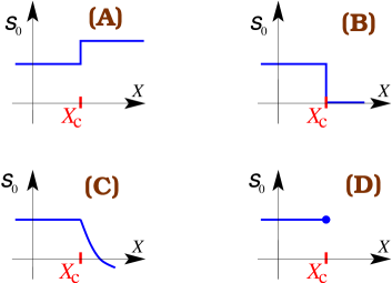
If we are in a topologically ordered phase, the negative intercept will by definition be equal to the topological entropy, . Figure 1 shows some possibilities of what can happen to as the 2D system is driven across a quantum phase transition away from the topologically ordered state, by varying a parameter across the critical value . In the parameter range where the system is in the topologically ordered phase, is fixed at a positive plateau ().
Case A shows a transition into another topologically ordered state with a different quantum dimension; jumps to another constant value . The other figures show transitions to non-topological phases. Case B shows a transition to a gapped state which is not topologically ordered – the intercept drops to zero. (Ref. CastelnovoChamon_topol-QPT_PRB08 treats an example.) Case C shows a transition into a non-topological phase, in which is nonzero but not constant. Finally, Case D shows a transition into a state where the leading term in the asymptotic behavior of is not linear, so that is undefined.
II.2 FQH wavefunctions on spheres
For finite-size studies of fractional quantum Hall physics, spherical and toroidal geometries are particularly popular when one wants to avoid complications due to the edge. We set notation by providing a rapid review of FQH wavefunctions on spheres Haldane_PRL83 ; HaldaneRezayi_PRL85 . We study electrons on a sphere of radius , subjected to the magnetic field provided by a magnetic monopole at the center of the sphere. The Dirac quantization condition requires the number of fluxes to be integral, where is the quantum of flux. If we measure length in units of the magnetic length , then the quantization condition is . The Landau-level orbitals are labeled either to or to . The wavefunctions in spherical coordinates are given by
There is no dependence on the azimuthal angle; the orbitals are each localized around a “circle of latitude”, with the orbital localized near the “north pole.” Basis states for the -electron wavefunctions are expressed in terms of the occupancies of these orbitals.
To define entanglements between two parts of the sphere, one has to first partition the sphere into and . We define block to be the first orbitals, extending spatially from the north pole out to some latitude, i.e., including orbitals through .
While neighboring orbitals do overlap, it is natural to think of the location where their amplitudes are equal, , as the “boundary” between the orbital and the orbital . This happens at angle
The boundary between partitions and is thus a circle of latitude at polar angle . The boundary length is
In finite-size spherical geometries, FQH states do not appear exactly at the filling fraction . Instead, the number of orbitals is related to the number of particles by:
where the shift is an integer determined by the FQH state Wen_shift . Although is insignificant in the thermodynamic limit, it can create an “aliasing” problem in numerical studies: different FQH states can compete at the same finite values of and .
II.3 Exact diagonalization
Our analysis is based on numerical exact diagonalization of Coulomb-like Hamiltonians projected onto appropriate Landau levels (lowest Landau level for and the second Landau level for ). We employ the spherical geometry described above. For this work, we have calculated wavefunctions up to 14 fermions and wavefunctions up to 20 fermions. To give an idea of the scale of these calculations, we note that for the wavefunctions at the Hilbert space dimension is 193498854, while for the wavefunctions at , it is 129609224. Dimensions are given here after reduction using the discrete symmetry under global flip.
We used the Lanczos algorithm to compute the system ground state. Calculations were performed on a PC cluster with 24 cores (AMD Opteron 265) and 48 Gbytes of memory. A Lanczos iteration typically requires up to 17h of cpu time for the largest Hilbert spaces. In our study of phase transitions, calculations are particularly time-intensive when the system is in or near a gapless phase, in which case the Lanczos procedure requires a larger number of iterations to converge.
II.4 Phase transitions
For FQH systems, the natural interaction parameter to vary is one of the Haldane pseudopotentials obtained by decomposing the interaction potential into channels specified by the relative angular momentum of the interacting particles Haldane_PRL83 ; HaldaneRezayi_PRL85 . We use interaction potentials whose pseudopotential is changed, while the other are fixed at the Coulomb value for that Landau level. We calculate and present wavefunction properties as a function of . Tuning of loosely represents variable aspects of FQH experiments, such as the thickness of the quantum well where the 2D electron gas resides.
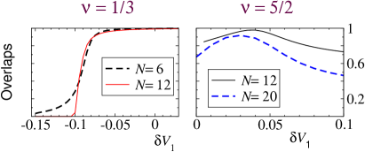
For the case, the exact Laughlin state is obtained for (short-range interaction), and continues to be a good description of the state for the Coulomb potential, . However, for negative , there is a quantum phase transition at some into a non-FQH incompressible state HaldaneRezayi_PRL85 . The overlap plots of Fig. 2 (left panel) shows the transition to be somewhere between and . The non-FQH state for presumably has charge-density-wave or Wigner-crystalline order HaldaneRezayi_PRL85 ; the details are not important for our purposes.
For , the overlaps (figure 2) suggest that the Moore-Read state is stable in some window of slightly positive (around ), and that there are transitions on either side of this phase to non-FQH phases Morf_PRL98 ; RezayiHaldane_PRL00 . The non-FQH phases are possibly a striped charge-density-wave phase on the left of the Moore-Read region and a composite fermi sea on the right RezayiHaldane_PRL00 .
II.5 Extrapolation for
The definition of the topological entanglement entropy , or the quantity in equation 1, involves two extrapolations: (1) to the thermodynamic limit, , and (2) to the asymptotic limit of the size of the block, i.e. . This double scaling limit can be approached via different possible extrapolation paths in the space. To describe the different extrapolation methods, we first rewrite the relation (1) for finite and :
| (2) |
We have ignored -dependence of and both - and -dependence of . Our experience with numerical wavefunctions indicate that these dependences are generally weak, at least for model FQH wavefunctions. Note that, even for topologically ordered model FQH states, the block entanglements are not linear in for finite (c.f. Fig. 1 in Ref. our-prl07 ). The reason is that is proportional to the square root of the area of the region, which is not proportional to the circumference in the curved geometry of the sphere.
In Sec. III, we consider the method used in Refs. our-prl07 ; our-pfaffian-entng , namely, performing the extrapolation first for each , and then using the resulting versus to extract or .
In Sec. IV we consider the extrapolation procedure in reverse order, namely, first extracting from finite-size versus dependences, and then taking the limit.
In Sec. V, we take the block to be half the system (which is a natural choice in a spherical geometry), . Examining the versus may be regarded as taking the two limits simultaneously.
II.6 The entanglement spectrum
Clearly, the complete spectrum of the reduced density matrix of a subsystem contains more information than any one number (such as the entropy of entanglement ) extracted from this spectrum. Extraction of additional information from the complete spectrum has been reported in several other condensed-matter contexts.
Ref. LiHaldane_PRL08 has empirically shown that, for FQH wavefunctions on a sphere, the spectrum of the reduced density matrix of one hemisphere can be related to the conformal field theory (CFT) describing the 1D edge of the FQH state. We exploit this notion in Sec. VI to show how quantum phase transitions appear in the so-called entanglement spectrum.
Another way of exploiting the complete spectrum of is via majorization comparisons, which we use in Sec. VII.
III Extrapolation for each block size
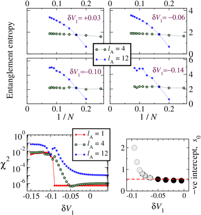
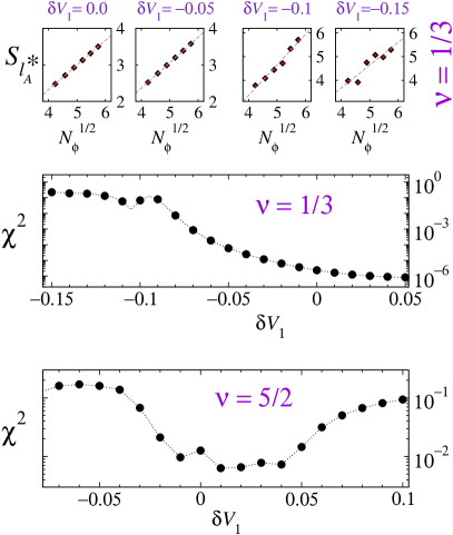
We attempt to employ the extrapolation method of Refs. our-prl07 ; our-pfaffian-entng , first extrapolating for fixed values of . From the versus plots in figure 3 (top 4 panels), we note that the extrapolation starts to lose meaning as one reduces beyond the presumed transition. This is made quantitative by estimating goodness-of-fit of the versus data to simple functions. The plotted estimates are obtained from trying ; any other reasonable function gives similar results. This versus curve can be regarded as one entanglement signature of the phase transition.
The jump in gets sharper for smaller . In particular, for it is distinctly localized at . This appears to provide a sharp estimate for the location of the transition. One tempting interpretation is that, since the system is large compared to a single orbital, for moderate is already a good indicator of the thermodynamic limit; hence the sharp jump.
One could still estimate extrapolates, disregarding the “noise” in the versus datapoints. The resulting points, plotted against , gives a line whose intercept is by definition . The estimates of , thus obtained, move away from the expected value of around the transition point. However, it is important to note that in the region , the estimates have relatively little meaning. First, there is the increasing scatter in the versus data, which makes the values unreliable. Second, we find that the versus curves are more and more curved as one increases further away from the Laughlin state. Given the uncertainties, we do not attempt to estimate error bars for . The point here is to note how loses meaning, in the large- region for which we have used shaded symbols in figure 3. Referring back to figure 1, the situation we have should be regarded more like case D and not like case C.
IV Dependence on circumference and area law
We now consider extrapolations in reverse order, i.e., first find a negative intercept for each by looking at the large- behavior at that , and only afterwards consider the -dependence. For topologically ordered model FQH states, the block entanglements have good linear dependences on the circumference , for any fixed .
Here we are of course interested in realistic wavefunctions, i.e., the ground states of Coulomb-like potentials. In figure 4, versus plots are shown for several , for states of 12 particles. It is interesting to note that the plots remain smooth as is increased past the transition; however they acquire curvature. As the dependence deviates from the linearity of model wavefunctions, extracting loses meaning. We do not attempt estimating . Instead, the deviation from linearity is shown through measures. The rise in again represents the quantum phase transition.
Note that this deviation from linearity does not necessarily constitute a violation of the area law, which is a statement about the thermodynamic limit. The deviation could instead indicate a stronger -dependence of the quantity in Eq. (2).
V Entanglement between equal hemispheres
We now consider entanglement between equal hemisphere-shaped and blocks, i.e., we use . According to Eq. (2), should depend linearly on the circumference . For the exact Laughlin state, an example is shown in Fig. 1 (inset) of Ref. our-prl07 . Here, we explore the fate of this linearity as a function of .
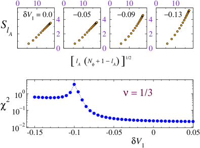
The top row in figure 5 plots against for several values at . The points acquire scatter as is increased, until it becomes meaningless to extract the intercept; the situation is similar to Section III (figure 3). This process is indicated by the curve (center panel) signifying the goodness of the linear fit.
The case (figure 5 bottom panel) similarly shows that the scatter is low (so that a linear versus fit is meaningful) only in the window of where the Moore-Read state describes the physics of the ground state.
A technical note: for even , the number of orbitals is odd and it is impossible to divide the sphere precisely into halves. In this case we keep orbitals in block , which nearly divides the sphere into halves, and use values for the entropy and for the circumference.
VI Entanglement spectrum and entanglement gap
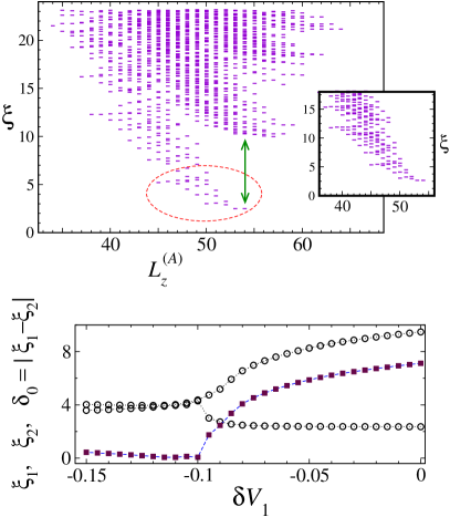
Following Ref. LiHaldane_PRL08 , we introduce the ”entanglement spectrum” as , where are eigenvalues of the reduced density matrix of one hemisphere. The eigenvalues can be classified by the number of fermions in the block, and also by the total “angular momentum” of the block. It was argued LiHaldane_PRL08 that the low-lying spectrum of the reduced density matrix for fixed , plotted as a function of , should display a structure reflecting the conformal field theory (CFT) describing the edge physics. In figure 6 this “CFT spectrum” is marked with an ellipse. For interactions at which the FQH state provides a good description of the physics, the CFT spectrum is well-separated by a gap from a higher “non-CFT” part of the spectrum.
As in Ref. LiHaldane_PRL08 , we denote the gap between the lowest two , at the value where the highest- member of the CFT spectrum occurs, as . In figure 6, this is the gap between the lowest two states at (marked by arrow). We study what happens to the spectrum as we tune the interaction away from the FQH state across a quantum phase transition. We quantify the change of the spectrum in terms of the quantity , defined above. (The quantities defined in Ref. LiHaldane_PRL08 , the gaps at other values, are expected to have similar dependence on .)
In figure 6 (lower panel), we plot as a function of the pseudopotential for the case. This clearly shows a dramatic decrease of the ”entanglement gap” around the region of the phase transition. The two levels in question are also individually plotted with open dots; there is a level crossing around . We note that for values of the CFT-like structure of the entanglement spectrum is lost so it is no longer meaningful to think of as the gap between CFT and non-CFT energy levels. A similar picture is observed for Moore-Read wavefunctions Haldane_unpublished .
VII Majorization
The concept of majorization involves comparison of two complete spectra. In the context of condensed-matter applications, it generally involves the comparison of two reduced density matrix spectra corresponding to the ground states of two Hamiltonians with slightly different parameters LatorreRicoVidal_PRA05 ; orus_maj ; calabrese_maj .
To define majorizaton, we consider two sets of real elements and sorted in decreasing order and satisfying . One says that the set majorizes the set if
This relationship is often expressed as . Obviously, if then , where is the von Neumann entropy.
In 1D quantum systems, the spectrum of the reduced density matrix for a spatial block has been argued LatorreRicoVidal_PRA05 ; orus_maj ; calabrese_maj to become more majorized as one moves along a renormalization group (RG) flow, away from an RG fixed point. As of now, there are no established general results for 2D quantum states.
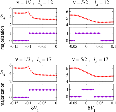
In figure 7, we examine majorization of reduced density matrices between ground states at different values of the pseudopotential . We show results for the system with particles, and the system with particles. For the system, we find that the eigenspectrum is continuously majorized as decreases down to the value , i.e., down to the phase transition region. In this region, the eigenspectrum of for each majorizes the eigenspectrum at a smaller (more negative) . For , the spectra are not majorized. This result is robust for different sizes () of the block. A similar picture emerges for the system; majorization occurs in a region roughly corresponding to where the ground state has the structure of the Moore-Read state. However, the effect is more fragile, e.g., the extent of values where the majorization is found, depends on the partition size () used. Note for filling that has a kink near the transition point. No such feature is seen for the case, neither in not in its derivative.
To summarize, we have demonstrated for that the region where majorization occurs coincides dramatically with the region where the system is in an FQH state; we no longer find majorization away from this phase. The situation is similar but less clear for . A full understanding is lacking at the moment, but several intriguing speculations present themselves. Most obviously, it is tempting to think of majorization being an indicator of quantum phase transitions. Second, since the reduced density matrix of a block of the sphere contains information about the physics of the quantum Hall edge LiHaldane_PRL08 , it is possible that our majorization results can be interpreted in terms of the evolution of the edge as a function of .
VIII Conclusions
We have presented a numerical study of how quantum phase transitions involving fractional quantum Hall states are manifested in entanglement measures and related quantities. We used three extrapolation methods to examine the double-scaling limit where the block entanglement intercept ( in equation 1) is defined. We showed that the breakdown of these extrapolation procedures signals the quantum phase transitions away from the topologically ordered incompressible FQH states. In addition, the entanglement spectrum was used in more detail in two different ways to characterize the quantum phase transitions, exploiting recently-developed concepts of CFT spectrum and majorization.
Our work opens up several new open questions and directions.
Since we have explored topological phase transitions on spherical geometries only, it would be instructive to look for analogous signatures on a toroidal geometry. Entanglement scaling behaviors are known in much less detail for FQH states on the torus, and further investigations are clearly needed.
Second, our results on majorization invite a thorough investigation of this concept, in general for two-dimensional systems and in particular both for 2D phase transitions and for topologically ordered states. It would appear that the knowledge necessary for putting our findings in context does not yet exist. The study of majorization, and the upper part of the reduced density matrix spectrum, also raises the question of other signatures of topological phase transitions one might yet extract from the full spectrum.
Finally, for topologically ordered states, it is promising to explore our three extrapolation methods, for extracting the topological quantity . In previous work with FQH states on spherical geometries our-prl07 ; our-pfaffian-entng , the focus has been on the first extrapolation procedure (section III). If the topological entanglement entropy is to be used to identify intricate FQH states and their CFT’s, improved methods of calculating are vital. Alternate extrapolation methods is one direction that needs to be explored in this regard.
Acknowledgements.
We acknowledge many discussions with and collaborative work with Kareljan Schoutens, and helpful discussions with B. A. Bernevig, P. Calabrese, C. Chamon, F. D. M. Haldane, E. H. Rezayi. OZ and MH thank the European Science Foundation (instans programme) for travel grants enabling parts of this work.References
- (1) L. Amico, R. Fazio, A. Osterloh, and V. Vedral, Rev. Mod. Phys. 80, 517 (2008)
- (2) M. Haque, O. Zozulya and K. Schoutens; Phys. Rev. Lett. 98, 060401 (2007).
- (3) O. S. Zozulya, M. Haque, K. Schoutens, and E. H. Rezayi; Phys. Rev. B 76, 125310 (2007).
- (4) H. Li and F. D. M. Haldane, Phys. Rev. Lett. 101, 010504 (2008)
-
(5)
X. G. Wen & Q. Niu; Phys. Rev. B 41,
9377 (1990).
X. G. Wen, Phys. Rev. B 40, 7387 (1989); J. Math. Phys. 4, 239 (1990).
M. Oshikawa & T. Senthil; Phys. Rev. Lett. 96, 060601 (2006). -
(6)
N. R. Cooper and N. K. Wilkin, Phys. Rev. B 60, R16279 (1999).
N. K. Wilkin and J. M. F. Gunn, Phys. Rev. Lett. 84, 6 (2000).
N. R. Cooper, N. K. Wilkin and J. M. F. Gunn, Phys. Rev. Lett. 87,
120405 (2001).
N. Regnault and Th. Jolicoeur, Phys. Rev. Lett. 91, 030402 (2003). N. Regnault and Th. Jolicoeur, Phys. Rev. B 69, 235309 (2004). -
(7)
M. Freedman, M. Larsen, and Z. Wang; Commun. Math. Phys. 227, 605
(2002).
S. Das Sarma, M. Freedman, and C. Nayak, Physics Today, July 2006, page 32.
A. Yu. Kitaev, Ann. Phys. 303, 2 (2003).
S. Das Sarma, M. Freedman, C. Nayak, S. H. Simon, and A. Stern, arXiv:0707.1889. - (8) A. Kitaev & J. Preskill; Phys. Rev. Lett. 96, 110404 (2006).
- (9) M. Levin & X. G. Wen; Phys. Rev. Lett. 96, 110405 (2006).
- (10) C. Castelnovo and C. Chamon, Phys. Rev. B 77, 054433 (2008).
- (11) A. Hamma, W. Zhang, S. Haas, and D. A. Lidar, Phys. Rev. B 77, 155111 (2008)
- (12) F. D. M. Haldane, Phys. Rev. Lett. 51, 605 (1983).
- (13) R. B. Laughlin, Phys. Rev. Lett. 50, 1395 (1983).
- (14) F. D. M. Haldane and E. H. Rezayi, Phys. Rev. Lett. 54, 237 (1985).
- (15) G. Moore and N. Read, Nucl. Phys. B360, 362 (1991).
- (16) J. I. Latorre, C. A. Lütken, E. Rico, and G. Vidal, Phys. Rev. A 71, 034301 (2005).
- (17) R. Orus, Phys. Rev. A 71, 052327 (2005).
- (18) B.A. Friedman and G. C. Levine, Phys. Rev. B 78, 035320 (2008).
- (19) S. Dong, E. Fradkin, R. G. Leigh and S. Nowling, JHEP05 (2008) 016.
- (20) A. G. Morris and D. L. Feder, arXiv:0808.1293.
- (21) S. Furukawa & G. Misguich; Phys. Rev. B 75, 214407 (2007).
- (22) C. Castelnovo and C. Chamon, Phys. Rev. B 76, 184442 (2007).
- (23) C. Castelnovo and C. Chamon, arXiv:0804.3591.
- (24) S. Iblisdir, D. Perez-Garcia, M. Aguado, J. Pachos, arXiv:0806.1853.
- (25) D. Gioev and I. Klich, Phys. Rev. Lett. 96, 100503 (2006).
- (26) M. M. Wolf, Phys. Rev. Lett. 96, 010404 (2006).
- (27) T. Barthel, M. C. Chung and U. Schollwöck, Phys. Rev. A 74, 022329 (2006).
- (28) W. Li, L. Ding, R. Yu, T. Roscilde, and S. Haas, Phys. Rev. B 74, 073103 (2006).
- (29) X. G. Wen and A. Zee, Phys. Rev. Lett. 69, 952 (1992).
- (30) R. H. Morf, Phys. Rev. Lett. 80, 1505 (1998).
- (31) E. H. Rezayi and F. D. M. Haldane, Phys. Rev. Lett. 84, 4685 (2000).
- (32) F. D. M. Haldane, unpublished.
- (33) P. Calabrese and A. Lefevre, arXiv:arXiv:0806.3059v1.