Feedback topology and XOR-dynamics in Boolean networks with varying input structure

Abstract

We analyse a model of fixed in-degree Random Boolean Networks in which the fraction of input-receiving nodes is controlled by the parameter $\gamma$. We investigate analytically and numerically the dynamics of graphs under a parallel xor updating scheme. This scheme is interesting because it is accessible analytically and its phenomenology is at the same time under control, and as rich as the one of general Boolean networks. We give analytical formulas for the dynamics on general graphs, showing that with a xor-type evolution rule, dynamic features are direct consequences of the topological feedback structure, in analogy with the role of relevant components in Kauffman networks. Considering graphs with fixed in-degree, we characterize analytically and numerically the feedback regions using graph decimation algorithms (Leaf Removal). With varying $\gamma$, this graph ensemble shows a phase transition that separates a tree-like graph region from one in which feedback components emerge. Networks near the transition point have feedback components made of disjoint loops, in which each node has exactly one incoming and one outgoing link. Using this fact we provide analytical estimates of the maximum period starting from topological considerations.

I Introduction

Biological networks are graphs representing the basic interactions between molecules in a living cell Barabasi and Oltvai (2004); Alon (2003); Hartwell et al. (1999); Bray (2003). They are generally composed of a fairly large number of elements and for this reason it is unfeasible to treat all the biochemical processes in detail. For example, a transcription network Oltvai and Barabasi (2002); Lee et al. (2002); Babu et al. (2004) of a simple cell counts some thousands of nodes, which represent the genes of a cell. Given the interaction structure, it is important to establish which genes are active in a given time or environment, or under a given stimulus. In order to fulfill this task, it is necessary to develop coarse-grained models for gene expression, such as discrete systems, in which variables on the nodes represent the (discretized) expression of single genes, and directed connections stand for their interactions Thomas (1973); Kauffman (1993). These abstract models are useful to study on general grounds the emergent cooperative behaviour of gene expression, as biological function is increasingly being recognized as emerging from global phenomena rather than from the expression of single genes Barabasi and Oltvai (2004); Guelzim et al. (2002); Isalan et al. (2008).

The simplest model of this kind are Random Boolean Networks (RBNs) introduced by S. Kauffman in 1969 Kauffman (1969). In this model, $N$ elements take binary values and interact with some random coupling functions. In the standard Kauffman model, the configuration of an element is set by Boolean functions whose values depend on a fixed number $k$ of inputs. The system is specified by its topology (a graph with $k$ inputs regulating each node), a synchronous updating scheme and the choice for the ensemble of Boolean functions (for an introductory review see Refs. Gershenson (2004); Aldana et al. (2003); Drossel (2007)). Technically speaking, the behaviour of the system is fully characterized by its cycles (or fixed points) and their basins of attraction. If a cycle contains exponentially many (in $N$) configurations, the behaviour is called chaotic. Otherwise it is called ordered. According to the original Kauffman interpretation, if the system is in a chaotic state, it cannot exhibit specific behaviour in response to external stimuli. More specifically, a realization of the model is interpreted as a genome and an attractor as a possible cell type (this particular interpretation is today considered out of date Ribeiro and Kauffman (2007)). If the corresponding cycle period is too long, this hypothetical cell type would never realize it. For this reason, networks of biological interest should lie between the ordered and the chaotic phase (the so-called critical networks Bastolla and Parisi (1997)), where attractor cycles are neither too short nor exponential.
There are two problems concerning Kauffman’s model in relation with genetic networks. First, the ensemble contains only graphs entirely made of feedback, while typically this is not the case of biological (e.g. transcription) networks, which usually have some “sensor” nodes that respond to external conditions Seshasayee et al. (2006); Luscombe (2004); Balaji et al. (2007). Thus, it is useful to modify the model and consider networks with well-defined input structure. The second problem is connected to the choice of the ensemble of Boolean functions. While on biological grounds it is difficult to characterize this class, from a mathematical viewpoint the choice of functions strongly conditions the behaviour of the model. Indeed, since most functions are constant, or “canalizing” Aldana et al. (2003); Drossel (2007) with respect to some variables, this creates an “effective topology”, which does not correspond to the underlying interaction graph. For this reason, the study of attractors in Kauffman networks is complex (for recent results see, for example, Paul et al. (2006); Samuelsson and Troein (2003); Drossel (2005)). Also the study of critical networks with canalizing Boolean functions leads to the conclusion that this choice does not decrease attractor sizes and render the model more well-behaved as previously expected Paul et al. (2006).

In this work, we address these questions in a controlled way, with the following choices. First, we work with a graph ensemble with a parameter that regulates the fraction of input nodes, as done in prvious studies that focused on fixed points Cosentino Lagomarsino et al. (2005b); Correale et al. (2006a, b); Cosentino Lagomarsino et al. (2006). Secondly, we choose to use the ensemble of xor or totally non- canalizing functions. In other words, we consider the situation in which all the existing links in the network have a role in the dynamics of real systems. The aim is to study the repercussions of the chosen topology on the dynamics and how this restricted selection of Boolean functions, in which the output changes if any one of the inputs changes its value, strictly relates these two aspects of the model. From the technical viewpoint, this dynamics has the advantage to be approachable with linear algebra using the finite Galois field $GF(2)$ Kolchin (1998); Caracciolo and Sportiello (2002), the set $\{0,1\}$ where addition between elements is equivalent to the logic xor and multiplication to the logic and.

Our main results are the following. With varying $\gamma$, we observe a phase transition, similar to the one observed in Kauffman networks, from a region characterized by an ordered dynamic behaviour to a region in which the dynamics is chaotic. From a topological point of view the same transition divides a region characterized by tree-like graphs from one in which extensive feedback is present. The structure of networks around the critical point appears simplified, in the sense that the feedback regions of this kind of networks are organized in simple disjoint loops. We use the topological structure of critical point networks to estimate the maximum period times. The paper is organized as follows. After giving the basic definitions in Section II, we present the main results in Section  III. In the last sections we discuss the results and the parallels with the scaling approach to general Kauffman networks Mihaljev and Drossel (2006).

II Definition of the model

We consider networks of $N$ nodes, of which only $M$ receive input, and define $\gamma=M/N$. Each of these regulated nodes receives inputs from exactly $k$ randomly and independently chosen other nodes. Consequently the in-degree is $k$ or $0$, while the out-degree distribution is binomial, and in the “thermodynamic” limit $N\rightarrow\infty$ and $\gamma$ constant is well approximated by a Poisson distribution of mean $k\gamma$,

$$p_{out}(\gamma k,n)=e^{-\gamma k}\frac{(\gamma k)^{n}}{n!}.$$

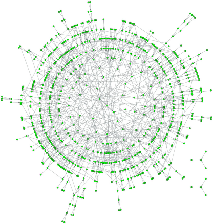
As a consequence, the graphs contain nodes with no output (leaves) and $N-M$ roots, i.e. variables without inputs (Fig. 1). This ensemble is conventionally used in diluted spin-glass models and constraint-satisfaction networks Mézard et al. (1987, 2003). The standard Kauffman graph ensemble can be obtained considering the special case $\gamma=1$ in which all variables are regulated.

Figure 1: A network with $N=9$, in-degree $k=2$ and $\gamma\simeq 0.55$. Red circles (colors online) indicate roots, blue circles leaves and green circles the inner nodes.

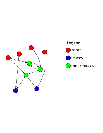
The graph ensemble is specified by a $M\times N$ connectivity matrix $A$ where $a_{ij}=1$ if the edge $j\rightarrow i$ exists, and zero otherwise. It is useful to arrange the columns of $A$ in order to reserve the first $M$ indices to the nodes that receive inputs. This matrix can further be divided into two submatrices $A=(S\;|\;R)$. $S$ is the $M\times M$ matrix that describes the interaction between regulated elements, while the columns of $R$ contain the information on the outputs of the free variables.

We consider a dynamics on the graphs of this ensemble, specified by assigning Boolean variables to each of the $N$ nodes and interactions through xor coupling functions. A global state $\vec{\sigma}$ is defined as the set of configurations assumed by all the nodes of the network. The initial conditions determine the state of the root nodes since they do not have input and their values remain fixed during the evolution. Root nodes are considered as external inputs and for this reason we can think that the initial conditions represent “the external world”. The configuration space, formed by all global states, contains $2^{N}$ states. Since the system is finite, starting from some initial global state, the deterministic dynamics leads to periodically repeated states, possibly after a transient time. In other words, the system performs a trajectory in the state space and eventually arrives to an attractor of length $T$, where the states are periodic in time. The attractor has length $T$ if $\vec{\sigma}(t+T)=\vec{\sigma}(t)$. We call this a $T$-cycle or a fixed point, in case of unitary length. The basin of attraction of an attractor is the set of global states that reach the attractor, including the attractor states. A transient state is a state that belongs to a basin but is not part of an attractor. The $N$-dimensional Boolean vector $\vec{\sigma}(t)$ can be written as $\vec{\sigma}(t)=(\vec{x}(t)\,,\,\vec{y}(t))$. The $M$-dimensional vector $\vec{x}(t)$ denotes the state of the regulated variables and the ($N-M$)-dimensional vector $\vec{y}(t)$ the (constant) state of the root variables ($\vec{y}(t)=\vec{y}(0)=\vec{y}$).
The synchronous update at time $t$ is determined by random xor functions, or, equivalently, by the linear operation in the Galois field $GF(2)$ Kolchin (1998); Cosentino Lagomarsino et al. (2006)

$$\vec{x}(t+1)=A\vec{\sigma}(t)+\vec{b}\;=S\vec{x}(t)+R\vec{y}+\vec{b},$$ (1)

where $\vec{b}$ is a random $M$-dimensional Boolean vector containing the information relative to the nature of regulating functions. The components $b_{i}$ of $\vec{b}$ are $0$ or $1$ with probability $\frac{1}{2}$. The evolved state after $t$ steps is

$$\vec{x}(t)=S^{t}\vec{x}(0)+\sum_{i=0}^{t-1}S^{i}(\,R\vec{y}+\vec{b}\,)=S^{t}\vec{x}(0)+\Sigma(t)(\,R\vec{y}+\vec{b}\,),$$ (2)

where $\Sigma(t)\doteq\sum_{i=0}^{t-1}S^{i}$ (the symbol $\doteq$ stands for a definition). One can observe from Eq. (2) that the dynamics is controlled by the topology through the interaction matrix. The peculiarity of the xor dynamics is that every change of one (or an odd number of) input in a function determines a change in the output. We shall demonstrate that feedback components of the graph are the only relevant region needed for characterizing the dynamic behaviour of the whole network.
The model introduced here bears some similarities and some differences with the Kauffman model. One difference is that the graph ensemble is not the same, as only a fraction of nodes receives input. However, as we will see, root nodes and feedback regions play the same role of nodes with a constant update function and so-called “relevant” nodes Flyvbjerg and Kjaer (1988); Bilke and Sjunnesson (2001) respectively, leading to an interesting parallel with more general Boolean networks Mihaljev and Drossel (2006). In the standard Kauffman model, the existence of frozen nodes (i.e. nodes under constant update functions, where the variables assume the same value on every attractor) denotes that some links are irrelevant to the dynamics and effectively modifies the topology in a way that is, in general, difficult to control. By contrast, the simplified model presented here enables to separate the discussion and the study of topology and dynamics, the features of the dynamics being a repercussion of the topology of the network. Note however that in our case the value of root nodes can change with the initial conditions in contrast with what happens to frozen nodes in Kauffman networks.

III Results

III.1 General features of XOR-dynamics

The discrete xor dynamics defined above allows to derive some simple general properties that will be used in the following.

Firstly, linearity implies that the cycles have a least common multiple (lcm) structure, where longer nontrivial cycles can be constructed by combining smaller ones. As a consequence, if a network shows a set $\{T_{i}\}$ of cycle lengths, then a cycle of length $T^{\prime}=\mathrm{lcm}\{T_{i}\}$ also exists.

From Eq. (2) a global state $\vec{\sigma}(t)$ belongs to a $T$-cycle if $\vec{\sigma}(T+t)=\vec{\sigma}(t)$, which gives the condition

$$\left[(1+S)\vec{x}(0)+R\vec{y}+\vec{b}\right]\in\ker\Sigma(T)\;,$$

i.e. the vector on the left hand side is sent to $\vec{0}$ by the function $\Sigma$ for some $T$. In the eventuality of $T=1$ the same condition becomes

$$(1+S)\vec{x}(0)=R\vec{y}+\vec{b}\;.$$

The fact that the dynamics can only have transients or cycles translates into the formula

$$S^{l+t_{m}}=S^{l}\;,$$ (3)

where $l$ is the smallest integer such as $\ker S^{l}=\ker S^{l+1}$ (the length of the longest transient) and $t_{m}$ is the maximum cycle length (without repetitions) for the map $\vec{x}\rightarrow S\vec{x}$. Indeed, after a transient period of at most $l$ steps, the dynamics becomes cyclic, i.e. identical configurations occur each $t_{m}$ steps (and $S^{t_{m}}$ is the identity matrix). This quantity can be related to the maximum cycle for the complete dynamics using the fact that $\Sigma(2t_{m}+l)=\Sigma(l)$, so that for any given initial condition,

$$\vec{x}(2t_{m}+l)=S^{l}\vec{x}+\Sigma(l)(\,R\vec{y}+\vec{b})=\vec{x}(l)\;,$$

which implies that the maximum cycle for the full dynamics is at most $T_{max}=2t_{m}$.

We now give a heuristic argument connecting the algebraic properties of $S$ with statistical properties of the dynamics. If $m(T)$ is the multiplicity of $T$-cycles, and $\mathcal{B}(T)$ is the number of configurations in the basin of attraction of each $T$-cycle, one must have

$$2^{N}=\sum_{T}\mathcal{B}(T)m(T)\;.$$

The elements belonging to a basin of attraction are built adding $\vec{z}\in\ker S^{l}$ to a fixed system state $\vec{x}$ of a $T$-cycle (Note that also elements $\vec{z}=\vec{0}$ are taken in consideration and thus $\vec{x}$ itself is considered part of the basin). Thus, each attractor of length $T$ has a basin of attraction whose dimension is $\mathcal{B}(T)=T\mathcal{B}(1)=T\,2^{d}$, where $d=\dim(\ker S^{l})$. To compute the probability of a cycle one has to provide an estimate for $m(T)$. From previous work Cosentino Lagomarsino et al. (2005b), we know that generally the average number of fixed points is $m(1)=2^{N-M}$, this can be also the typical value, depending on the graph ensemble and the value of $\gamma$. Since adding a fixed point to the elements of a $T$-cycle leads to a cycle of the same length, $m(T)$ has a prefactor $m(1)$. Supposing that the contribution of the longer cycles is of order one, one can write, $m(T)\sim m(1)$, or in other words the multiplicity of cycles can be estimated using the number of fixed points. In this hypothesis, the probability $p(T)$ that a state is in the basin of attraction of a $T$-cycle is

$$p(T)=\frac{1}{2^{N}}\mathcal{B}(T)m(T)\simeq 2^{d-M}T\;.$$ (4)

Note that this estimate holds only for the values of $T$ that are possible. If $T_{max}$ grows faster than $M$, $\sum_{T}T\simeq T_{max}$ implying that $P(T)$ will be concentrated on $T_{max}$. Equation (4) has a practical implication for simulations: given a realization of a network, it enables to simulate only few initial conditions to find the value of $T_{max}$ that is reached with highest probability. These facts will help understanding some dynamic features of the networks around the critical line.

III.2 Simulations

We will now turn our attention to direct simulations of the model presented in Section II. In these simulations one has to sample a number of ensemble graphs, and for each graph, a number of random initial conditions. The choice of the average performed and the quantity of interest leads to the definition of different observables.

The simplest observables relate to the fixed points of the dynamics. Figure 2.a shows the probability of finding at least one fixed point as a function of the parameter $\gamma$. Fixed points are typically exhibited for low values of $\gamma$ while they become rare for higher values, with a sharp threshold in between. One can notice that increasing system size makes more evident the two distinct regimes. Another way of presenting this result is given in Fig. 2.b, which shows the variance of $p(1)$ depending on $\gamma$. This plot has a peak whose maximum value shifts with increasing number of nodes. Accurate location of the transition point in Figs.  2.a and 2.b is rendered difficult by the fact that for larger system sizes, where the results should be more reliable, sampling efficiently the initial conditions becomes difficult.

(a)

(b)

Figure 2: Simulations of dynamics: Fixed points. (a) Probability of finding at least one fixed point for different values of $N$ ($k=3$). The probability drops down after a certain value of $\gamma$. (b) Variance of the probability of observing one fixed point as a function of $\gamma$. The plot is obtained by averaging the fraction of $10^{3}$ random initial configurations reaching a fixed point (on a fixed graph) over $10^{3}$ graph realizations at a given $\gamma$.

Figure 3: Simulations of dynamics: Long cycles. The plot presents the fraction of periods larger than the cutoff ($10^{6}$). At $N$ and $\gamma$ given, we sampled $10^{3}$ random networks and for each network we evaluated $10$ initial conditions.

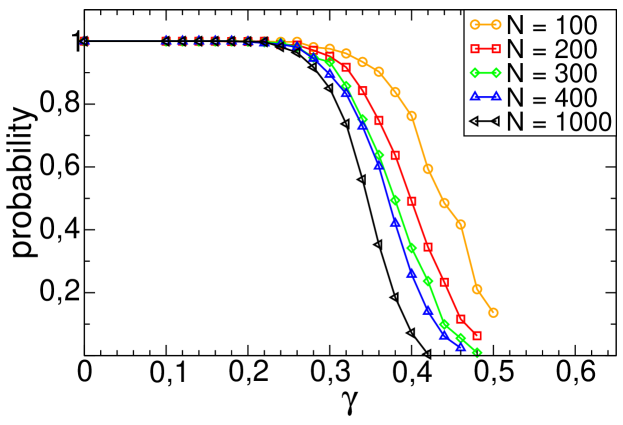
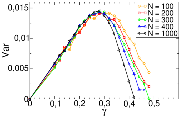
These results show signatures of a dynamical transition point $\gamma_{c}^{d}$ which marks the border between a region with typically fixed points and a region where cycles dominate on fixed points (for recent studies on the critical transition between chaotic and ordered phase in Kauffman networks see, e.g., Andrecut, M. and Kauffman, S. A. (2008)). According to Eq.  4, for $T=1$, the shape of the curves indicates that $d$ becomes significantly different from $M$ after a certain value of $\gamma$. In the large system limit, if $d\ll M$ one expects that $p(1)$ is negligible and the probability of finding at least one fixed point drops to zero. At the transition point the probability of a fixed point and its variance should drop to zero in the thermodynamic limit. The effects of finite size are evident as the measured transition point strongly depends on the system dimension. We will investigate these effects later (Section III.3). Note that the fraction of fixed points just below the threshold decreases unexpectedly with $N$. However, this has no physical meaning and is connected to the fact that the number of initial conditions is kept constant and consequently larger systems are increasingly under-sampled.

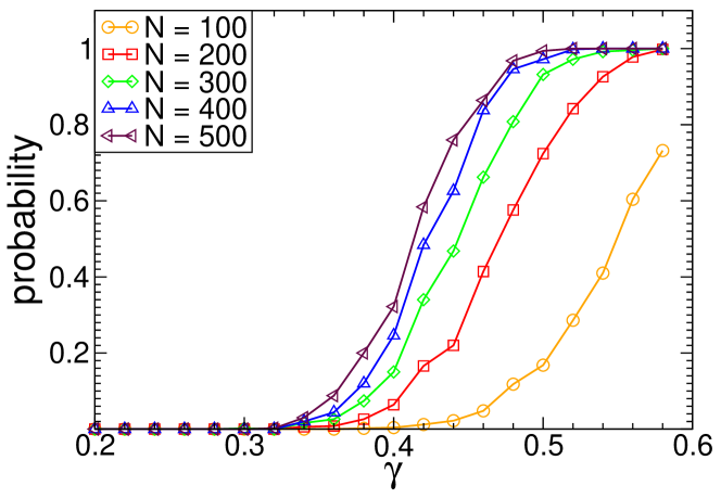
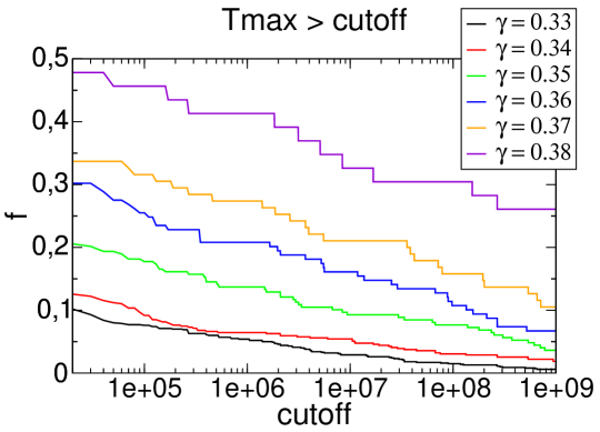
The same transition is visible by quantifying the length of cycles. However this task is computationally hard already for $N\simeq 100$, which strongly limits this kind of simulations. Indeed, to implement these simulations, it is necessary to impose a cutoff on the length of the maximum period observed. Figure 3 shows the fraction of networks with a period larger than the cutoff imposed, given $N$ and $\gamma$. This quantity grows rapidly beyond a characteristic parameter value that changes even more with the system dimension, and the transition point is difficult to locate precisely. Hence, it is necessary to find effective methods to investigate the dynamics and this problem will be discussed in Section  III.5 after having studied the feedback topology of graphs in correspondence with the transition.

III.3 Feedback topology and Leaf Removal algorithms

In this section, we analyze the topology of the graphs. The question that we want to address is whether the dynamic transition is connected to a change in the feedback topology of the underlying graphs.

To study the feedback regions we use three modified versions for directed graphs of the Leaf Removal (LR) decimation algorithm Mézard et al. (2003); Bauer and Golinelli (2001). A graph decimation technique consists in erasing iteratively nodes and links with some specified prescriptions. The variants we implemented remove tree-like parts of the graph, leaving the components with feedback. Network regions not removed by the algorithms are called feedback core of the graph or simply core. It is possible to study analytically the behaviour of the algorithms in the mean-field approximation Weigt (2002), considering for example the fraction of nodes in the core. The LR algorithms define a dynamics for the probability $p_{n}(t)$ that a regulated node has $n$ inputs at iteration $t$, (i.e. of having $n$ ones on a row of the matrix $S$), and for the probability $f_{n}(t)$ that a node has $n$ outputs at iteration $t$ ($n$ ones on a column of $S$). We study LR algorithms analytically with mean-field equations and compare with numerical simulations. As we will discuss, this approach is related to the scaling approach  Mihaljev and Drossel (2006) to general Kauffman networks, where one can write and analyze scaling equations for the numbers and fluctuations of nodes receiving input from a given number of frozen nodes.

Figure 4: Leaf Removal algorithms. (a) Iterations of LRu for the graph presented in Fig. 1 . The LRu removes iteratively the non regulating variables and their links (light grey nodes and dotted arrows). In this case the algorithm stops after two steps. (b) Iterations of LRd. The LRd removes iteratively the regulating variables that are not regulated and the associated links (light grey nodes and dotted arrows). Only one step is possible in this case. (c) Iterations of LRb. First the LRu is applied and then all non-regulating nodes are taken off with the LRd.

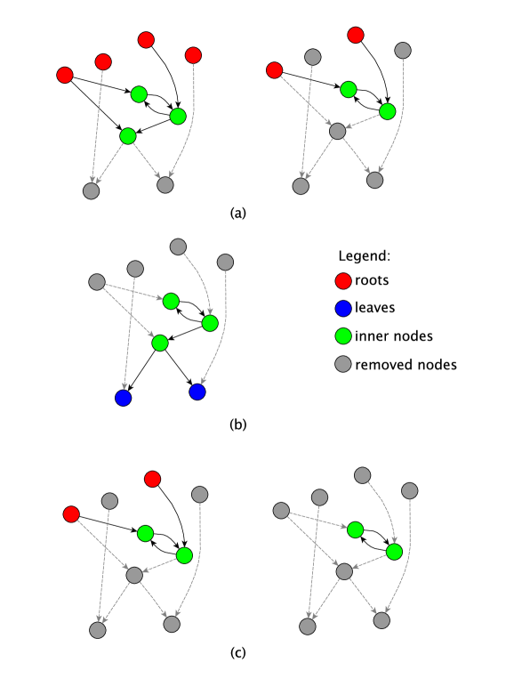
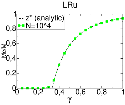
The first LR variant we analyze is the so called Leaf Removal Up (LRu) Cosentino Lagomarsino et al. (2006). In each step of this algorithm the variables without outgoing links (the leaves) are removed together with its incoming links. The procedure is iterated until each variable has at least one outgoing edge (Fig. 4.a). As a consequence of the removal of links, the distribution $f_{n}$ of the outgoing links changes after each iteration $t$, giving rise to fluxes that can be expressed by first-order mean-field equations for $f_{n}(t)$ (see Ref. Cosentino Lagomarsino et al. (2006) and Appendix  A). The solution of the mean-field flux equations is:

$$\begin{cases}f_{0}(\bar{t}\,)=-\bar{t}+e^{-\lambda(\bar{t}\,)}\\ f_{n}(\bar{t}\,)=e^{-\lambda(\bar{t}\,)}\frac{\lambda(\bar{t}\,)^{n}}{n!}\;,\qquad n>0\;,\end{cases}$$

where $\bar{t}=t/M$ and $\lambda(\bar{t}\,)=\gamma k(1-\bar{t}\,)$. The algorithm stops at the reduced time $\bar{t}^{*}_{up}$ and the number $M_{c}^{up}$ of remaining nodes is

$$M_{c}^{up}=Mz^{*}_{up}\;,$$

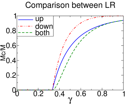
where $z^{*}_{up}=1-\bar{t}^{*}_{up}$ is a function of $\gamma$ and represents the fraction of nodes belonging to the LRu core on the total of regulated nodes. Figure 5.a compares the analytic curve for $z^{*}_{up}$ as a function of $\gamma$ with numerical results. Varying $\gamma$, there is a singularity which is a signature of a phase transition between a region characterized by graphs entirely removed by the algorithm ($z^{*}_{up}=0$) and a region in which the amount of remaining nodes after the process augments when $\gamma$ is increased. These regimes are separated by the “critical point” $\gamma_{c}^{up}=k^{-1}$ found with mean field equations.

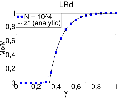
The second variant we analyze is the Leaf Removal down algorithm (LRd) Maffi (2005-2006), which, in a similar way as above, removes iteratively the nodes with no incoming links, together with their outgoing edges, until there are no more roots (see Fig. 4.b). The mean-field flux equations (shown in Appendix A) for the distribution of incoming links $p_{n}(t)$ have solution

$$\begin{cases}p_{0}(z)=(z-1)+(1-\gamma z)^{k}\\ p_{n}(z)=\left(\begin{array}[]{c}k\\ n\end{array}\right)(\gamma z)^{n}(1-\gamma z)^{k-n}\;,\qquad n>0\;,\end{cases}$$

where $z=1-\bar{t}$. When the algorithm halts the amount of nodes in the LRd core is given by

$$M_{c}^{down}=Mz^{*}_{down}\;.$$

The critical value $\gamma_{c}^{down}=k^{-1}$ divides the networks with a non-vanishing core in the large $N$ limit from the ones that are removed by LRd. The plot of $z^{*}_{down}(\gamma)$ is presented in Fig. 5.b and compared with simulations.

The last version of LR we consider is the combination of LRu and LRd which we call Leaf Removal both (LRb). From the point of view of the dynamics this algorithm first removes all the nodes which do not regulate the core and successively it removes the set of nodes that are fixed, at most after a transient time, the initial conditions given. From the topological viewpoint it leaves all and only the nodes involved in feedback cycles (Fig. 4.c). It can be checked that a single iteration of LRu and LRd is sufficient for this. The LRu algorithm stops at a matrix with $M_{c}^{up}$ rows having $k$ entries and whose remaining rows are empty. When LRd is applied to this matrix, elimination of all empty rows and columns leaves with $M_{c}^{both}=M_{c}^{up}z^{*}_{down}=Mz^{*}_{down}z^{*}_{up}$ nodes, and the following per-row and per-column probabilities of $n$ entries

$$\begin{cases}p_{0}=f_{0}=0\\ p_{n}=(z^{*}_{down})^{-1}\left(\begin{array}[]{c}k\\ n\end{array}\right)(\gamma z^{*}_{down})^{n}(1-\gamma z^{*}_{down})^{k-n}\\ f_{n}=(z^{*}_{up})^{-1}e^{-\lambda(\bar{t}^{*}_{up})}\frac{\lambda(\bar{t}^{*}_{up})^{n}}{n!}\;.\end{cases}$$ (5)

After the application of the algorithm, the distribution of both the outgoing and the incoming links has changed with respect to the initial network. In particular, no nodes without incoming/outgoing links may remain. In this case $z^{*}_{both}\doteq z^{*}_{down}z^{*}_{up}$ and $M_{c}\doteq M_{c}^{both}=Mz^{*}_{both}$ The core becomes extensive (order $N$) above the critical value $\gamma_{c}^{both}=k^{-1}$ (Fig. 5.c).

(a)

(b)

(c)

(d)

Figure 5: Phase transition for LR algorithms ($k=3$). The dashed lines represent the fraction of nodes removed by LR up (a), LR down (b) and LR both (c) calculated for different values of $\gamma$. Squares are numerical results for graphs with $N=10^{4}$ nodes and blue triangles in (c) are the simulations for $N=5\cdot 10^{4}$. Each point is obtained averaging $10^{4}$ simulations. Error bars are smaller than the dimension of the points. The discontinuity of the derivative points to the emergence of an extensive feedback core at $\gamma=\frac{1}{3}$. (d) Comparison of analytic curves for the three variants of the algorithm.

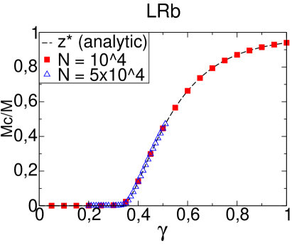
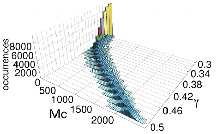
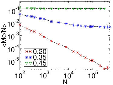
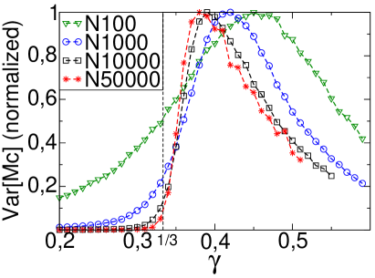
The analytical approach described so far evaluates the mean value of the number of nodes in the core, in the thermodynamic limit $N\rightarrow\infty$. In order to access the fluctuations around this value we use direct simulation. The shape of the distributions changes significantly with varying $\gamma$ and number of elements. Figure 6.a shows the distributions of $M_{c}$ with varying $\gamma$. Below the critical value, $M_{c}$ is condensed around zero, i.e. the graphs are typically close to being tree-like. Near the transition, the distributions have broad tails, and for $\gamma\gg\gamma_{c}$ they become symmetric around the value found with mean- field LR equations. This phenomenology is typical of phase transitions. In brief, the results show the presence of a phase transition, with varying the order parameter $\gamma$, between a region of typically tree-like graphs and a region of extensive feedback loops. These conclusions hold independently from the in-degree value $k$. Figure 6.c shows the consequence of finite sizes on the LRb algorithm on the transition: the peak of the variance plot indicating the transition point is shifted to greater values and, increasing the system dimensions, it slowly approaches the value $k^{-1}$. Even for systems with more than $10^{4}$ nodes, the critical point does not reach the analytically determined value. We call $\gamma_{e}$ the maximum of the variance of $M_{c}$ i.e. the effective critical value of $\gamma$ at finite system size ($\gamma_{e}\longrightarrow\gamma_{c},N\rightarrow\infty)$. In the region $\gamma_{c}\leqslant\gamma\leqslant\gamma_{e}$, a residual LRb core is observed and, as we will see, this affects the dynamics. Thus, for small networks, $\gamma_{e}$ does not distinctly separate the region characterized by tree-like graphs and the one defined by feedback regions which are present also before this value. This can be also observed in Fig. 6.b which presents the scaling of $M_{c}/N$. At a value of $\gamma=0.35$, $M_{c}$ may seem to be a sub-extensive quantity. However, increasing $N$ it appears clear that the core is extensive, as the LR equations predict. Taking simulations of very large systems (up to $5\cdot 10^{5}$ nodes), values of the fraction of remaining nodes in the core are comparable with which ones obtained from the analytic calculation.

III.4 Feedback structure at the transition

Let us now take a closer look at what happens around the critical point of LR algorithms. Figure 5.d shows that the three variants of LR have a different trend just after the transition value. Defining $\epsilon=\gamma-\gamma_{c}$, for small $\epsilon>0$ the rescaled times of arrest $z$ (i.e. the solutions of the equations $f_{0}(z^{*}_{up})=0$ and $p_{0}(z^{*}_{down})=0$, see Appendix  A) become

$$z^{*}_{up} \simeq 2k\epsilon(1-2k\epsilon)\simeq 2k\epsilon$$

$$z^{*}_{down} \simeq \frac{2\epsilon k^{2}}{k-1}(1-2\epsilon k)\simeq\frac{2\epsilon k^{2}}{k-1}$$

and for LRb:

$$z^{*}_{both}=z^{*}_{up}z^{*}_{down}\simeq\frac{4k^{3}}{k-1}\epsilon^{2}=\frac{4k^{3}}{k-1}(\gamma-\gamma_{c})^{2}\;.$$

These functions are continuous at the transition but not all their derivatives are. The discontinuity in $z^{*}_{both}$ is of greater order than the others, signature of transitions of different orders.

(a)

(b)

(c)

(d)

Figure 6: Feedback core. (a) Three-dimensional plot showing the histogram of the LRb-core size $Mc$ for different values of gamma (for $k=3$, $N=10^{4}$, and $10^{4}$ different networks, colors online). (b) Fraction of nodes in the LRb core. Points represent the averaged values resulting from simulations (ensembles composed by $10^{4}$ networks or $10^{3}$ for large systems) for different values of $\gamma$: 0.20 (red online), 0.35 (blue online) and 0.45 (green online). (c) Variance of the fraction of the number of nodes belonging to the core. (d) Histogram of the number $n$ of connected components of the core at varying $N$. For fixed values of $N$ the number of connected parts does not remarkably change remaining around the critical value of $\gamma$ (right). $10^{4}$ iterations for each value of $N$ are simulated.

We will now consider the topology of networks with $\gamma\simeq\gamma_{c}$ (critical networks). Starting from Eqns.  (5) we can write

$$f_{1} = \frac{1}{z^{*}_{up}}e^{-\lambda(z^{*}_{up})}\lambda(z^{*}_{up})\simeq e^{-2k\epsilon}\simeq 1-2k\epsilon+O(\epsilon^{2})$$

$$p_{1} \simeq (1-\frac{2k\epsilon}{k-1})^{k-1}\simeq 1-2k\epsilon+O(\epsilon^{2})\;,$$

concluding that $\frac{f_{2}}{f_{1}}\sim\epsilon$ and $\frac{p_{2}}{p_{1}}\sim\epsilon$. This means that, near to the transition point and at the thermodynamic limit, core matrices typically have one entry only per-column and per-row. In other words, they are permutations of the identity matrix (and consequently they are invertible). Thus, we can think of the residual (LRb) core as a particular Kauffman network with in-degree one Drossel (2007); Flyvbjerg and Kjaer (1988). There is, however, an important difference. In Kauffman networks with in-connectivity one, a node can have more than one outgoing edge, while in this case all nodes in the core must regulate exactly one element; there are no nodes without output (otherwise they would have been removed by the algorithm).

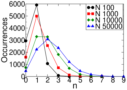
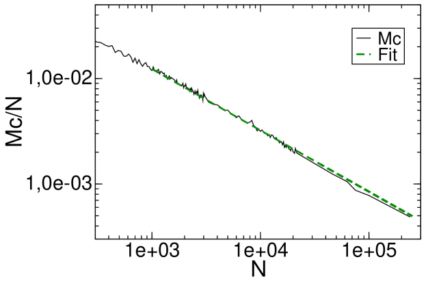
Having one entry per column and per row, core matrices correspond to graphs in which all nodes have (typically) one input and one output, and they show a structure with simple loops disconnected from each other (Figs. 7.b and 7.c). Simulations suggest the presence of several disconnected components that increase in number when the dimension $N$ of the system increases. With growing $N$, the number of tree-like graphs, as well as the number of cores with only one connected component, decreases (Fig. 6.d). The organization in disconnected loops does not depend on the in-connectivity degree $k$. The number of nodes in the core of critical networks scales as $N^{\zeta}$ with $\zeta\simeq 0.4$ (Appendix B).

(a)

(b)

(c)

Figure 7: Structure of a critical core. (a) shows a realization of a simulated network with $N=10^{3}$ and $M=333$ (potential isolated nodes are not depicted). It can be noticed that each regulated node receives exactly $k=3$ inputs. The structure is highly simplified after the application of LRb: only three disjoint simple loops are present (b). Panel (c) reports another typical chain structure of a core made of a single connected component (the starting graph had $N=100$ and $M=33$).

III.5 Connecting feedback topology and dynamics: reduced dynamics

Since topology and xor dynamics are strictly related, one would expect that the feedback topology transitions have a repercussion on the evolution of states. We first observe that, around the transition point, the matrices are invertible, hence $d=0$ (Section III.1). From this, the probability of having at least one fixed points falls down at the transition. On the other hand, before the transition one expects to have only fixed points, because of the tree-like structure of graphs. We can rearrange the indices of the matrix $S$ and place leaf variables (erased by LRu) in the first indices and roots (erased by LRd) in the lasts. In this way it takes the form Cosentino Lagomarsino et al. (2006):

$$S=\left(\begin{array}[]{c}\mathcal{L}\\ \hline\cr\begin{array}[]{cc}0\quad\phantom{a}&\begin{array}[]{|ccc}&&\\ \phantom{AB}&\mathcal{C}&\\ &&\end{array}\end{array}\\ \hline\cr\begin{array}[]{cc}\begin{array}[]{cccc}\phantom{a}&\phantom{a}&0&\phantom{a}\end{array}&\begin{array}[]{c|c}\phantom{a}&\>\mathcal{R}\end{array}\end{array}\end{array}\right)\;.$$

Nodes belonging to the LRb core are collected in the sub-matrix $\mathcal{C}$ which has $Mz^{*}_{both}$ rows. Applying $S$ to a vector of the form $\vec{x}(t)=(\vec{l}(t)\,,\,\vec{c}(t)\,,\,\vec{r}(t))$ (see Eq. (2) ) one concludes that the evolved state of roots, $\vec{r}(t)$, is fixed only by initial conditions and remains constant. The nodes $\vec{c}$ belonging to the LRb core are determined by both $\vec{r}$ and $\vec{c}$ itself. Finally, the configuration of leaf nodes $\vec{l}$ is established by all the variables and is not affected by feedback. Thus, the behaviour of the whole dynamics can be deduced from the state of the core. For these reasons, simulations of the dynamics restricted to the core (reduced dynamics) are sufficient to evince the salient features of the dynamics. Using this fact, we are able to simulate networks with up to $10^{3}$ nodes with a large statistic. On the other hand, obtaining data in the chaotic region is very difficult also using the reduced dynamics (see Fig. 8).

Figure 8: Fraction $f$ of networks which have a $T_{max}$ greater than a cutoff. Simulations made for networks with $N=999$ and $k=3$. From $\gamma=0.33$ to $\gamma=0.38$ we respectively simulated 1000, 589, 284, 149, 95, 46 different realizations of the model.

Nevertheless, the region immediately after $\gamma_{c}$ is interesting, because it carries the consequences of the simplified core structure in the topology. The equations for critical core variables are special cases of Eq. (1) when each node $i$ receives one input from node $j(i)$:

$$c_{i}(t+1)=c_{j(i)}(t)+b_{i}\;,$$

In case the core is a single component, then the maximum period length $T_{max}$ will be approximately equal to $M_{c}$. Since, near the transition, core matrices are invertible Eq. (3) becomes $S_{c}^{t_{m}}=1$ ($l=0$). The condition to have the maximum period is

$$\vec{c}(T_{max})=S_{c}^{T_{max}}\vec{c}(0)+\Sigma(T_{max})\vec{b}=\vec{c}(0)\;.$$

The matrices $S_{c}$ are also permutation matrices with dimension $M_{c}\times M_{c}$ and thus $S_{c}^{M_{c}}=1$. Since $\Sigma(2M_{c})=0$, the maximum period achievable is $T_{max}=2M_{c}\sim M_{c}$. In case the core is formed by several disconnected chains, the maximum period of the whole network can be computed as the least common multiple of the period of each single loop (Appendix C).

IV Discussion and conclusions

In this work, we considered a model of Random Boolean Networks related to Kauffman networks. The model has the objective to investigate on abstract grounds some features that are important in biological networks, mainly (1) the presence of nodes which regulate but are not regulated, existing in empirical transcription networks, and (2) the correspondence between topology and dynamics. For the latter reason we chose to use a xor dynamics to define the interaction between elements. We have shown that in this model the dynamical aspects characterizing the length of cycles and their basins of attraction are direct consequences of the topological feedback structure of the underlying networks, which we study with graph decimation algorithms (LRs) on a fixed in-degree ensemble of graphs.
We identified a dynamical and topological phase transition with varying input structure of the graphs modulated by the parameter $\gamma$ (the fraction of the input-receiving nodes). Direct numerical simulations of the dynamics (Figs. 2 and 3) suggest the presence of a phase transition where long cycles emerge. Correspondingly, a topological phase transition separates a tree-like graph region from one in which extensive feedback components are present. Different Leaf Removal algorithms that remove the upstream tree-like regions, the downstream ones, or both, have the same critical point $\gamma_{c}=k^{-1}$, which we locate analytically and numerically. The dynamic transition is found numerically at a critical value that is close to $\gamma_{c}$, but strongly influenced by finite size effects. Since networks below the transition typically exhibit fixed points, and this behaviour is correlated with the tree-like structure of these graphs, we identify the dynamic transition point with $\gamma_{c}$ in the thermodynamic limit. Thus, despite of the large finite-size effects which make the simulations difficult, our results lead to the conclusion that the topological and dynamic transitions are the same.
This result is only valid for the ensemble of functions under consideration. Dynamics with a more general class of functions should present a different critical point. However, the value of the nodes removed by LRd is fixed after a transient time, independently from the dynamics chosen, because the fact that nodes receiving inputs from the topological core depend just on the the state of the core is not conditioned to the class of functions. The relevant dynamical part of the network must be a subset of this the core, and a different choice of update rules moves the dynamical transition away from the $\gamma_{c}$. It is simple to imagine that with a more general class of functions one can still observe fixed points for values of $\gamma\gtrsim\gamma_{c}$. Thus, the topological critical point represents a lower bound for the dynamical critical point.
Above the transition (Fig. 3) the presence of an extensive feedback region induces chaotic dynamics, characterized by exponential cycles (order $2^{M_{c}}$ with $M_{c}\sim O(N)$). In this case, the initial conditions, and thus the influence of the external world (represented by the state of sensor nodes in the fraction $1-\gamma$), do not affect the dynamics. For this reason, studying the features of networks away from the transition is only relatively interesting.
The most interesting region to study is the transition point, where the dynamics can be at the same time nontrivial and under external control. At this point, our analytical mean field theory predicts that the structure of feedback components in the graph is simple. Feedback components (independently from the in-degree) show an elementary modular organization in simple disconnected loops, found in simulations (Fig. 7) and predicted by the analytical approach. In turn, this feedback structure transposes to a modular dynamics, which can be completely characterized by the lcm structure of periods. We give an analytical (large $N$) prediction for the maximum cycle achievable. Comparing with (small $N$) simulations (Fig. 11), the distribution of the maximum cycles is wide but, with increasing dimension of the system, the estimate becomes increasingly reliable and comparable with the prediction. This point might have an interest for the modeling of empirical biological networks (which have $N$ of the order of a few thousand). Indeed, at these “realistic” system sizes, this point corresponds to an interval with a finite span, because of finite-size effects, as it happens with Kauffman networks Socolar and Kauffman (2003).
It is interesting to make a comparison between the model used here and the behaviour of Kauffman networks with no input structure in the underlying graph and general Boolean functions. In the latter model, the dynamics is entirely controlled by so-called relevant nodes Flyvbjerg and Kjaer (1988); Bilke and Sjunnesson (2001) which have been the subject of many studies Socolar and Kauffman (2003); Kaufman and Drossel (2006); Krawitz and Shmulevich (2007); Bastolla and Parisi (1998a). In networks between the chaotic and the stable phase, they spontaneously organize into disconnected clusters whose number increases logarithmically with the system size Bastolla and Parisi (1998b); Kaufman and Drossel (2006). Most of relevant clusters are simple loops. The number of relevant nodes in critical networks scales as $N^{1/3}$ in the limit $N\rightarrow\infty$ Socolar and Kauffman (2003). As recently found by Drossel and coworkers Kaufman and Drossel (2006); Kaufman et al. (2005); Mihaljev and Drossel (2006), since the relevant part constitutes only a vanishing portion of the network, the topology of Kauffman networks is most likely very different from the topology of real biological networks, such as genetic regulatory networks, where one would expect that the majority of nodes is relevant or at least not always frozen.
As anticipated in Section II, there exists an analogy between relavant components of Kauffman networks and the LRb core of the $\gamma$ model. We find that the critical core has a modular structure and the amount of disconnected loops increases as the system size grows.
Considering the scaling approach of Mihaljev and coworkers Mihaljev and Drossel (2006), it is interesting to observe the close correspondence between an xor Kauffman network with an imposed fraction of $1-\beta$ of constant functions and the model studied here. In this case, their approach would give a transition between frozen and chaotic phase located at $\beta_{c}=1/K$ in the parameter space. Note that, however (since no xor functions are constant) the only way to vary $\beta$ in our case is to change the ensemble of graphs, i.e. vary $\gamma$, and allow for a input-output structure of the network. The difference between the two approaches is acting directly on the topology (more specifically, on the fraction of input nodes) instead of modifying the graph with the introduction of constant functions. The same reasoning suggest that this transition point we find is a lower bound for Kauffman networks with a fraction $1-\gamma$ of constant functions and a general ensemble of functions.
In spite of this analogy, simulations show that the number $M_{c}$ of nodes belonging to the core of critical networks scales as $N^{\zeta}$ with $\zeta\simeq 0.4$ (see Appendix B) that is different from the scaling exponent found for relevant components in critical Kauffman networks (discussed for example in the same study of Mihaljev and coworkers, Mihaljev and Drossel (2006)). The error on the fit seems to be small enough to exclude a discrepancy of $0.1$ in the exponent but it is possible that this deviation between the two models derives from the fact that we have accessed this quantity by numerical work, and thus are limited by system size (we tested up to 250.000 nodes). On the other hand, we can also speculate that this difference derives from the fact that the topology of the underlying graphs in the two models is not the same. Indeed, in the case of a general Kauffman network, nodes may become frozen because some of their inputs are connected to a frozen node, and the resulting function is constant. Thus, frozen nodes do not have strictly zero in-degree as in the $\gamma$ model. In our case, this cannot happen, as the topology is strictly controlled. In other words, the quantity $M_{c}$ describes the size of the feedback region that only for the $\gamma$ model with xor dynamics coincides with the relevant dynamic region. Studying the simplest possible case of this model has the further advantage of elucidating in detail some of the phenomenology connected to the properties of the critical core, its modular structure and the amount of disconnected loops, and thus providing an estimate for the size of the largest cycle in the dynamics.
In conclusion, while simplified, the $\gamma$ model gives an insight into the role of the input-output structure in the whole-network dynamics, which is relevant for gene networks. Direct application to concrete problems concerning regulatory networks would require generalizing the approach to more realistic representations for the input functions and graph ensembles Bassetti et al. (2007). In particular, for what concerns the dynamics, our results on the role of the emerging extensive feedback core, which apply to xor functions, could be extended to the study of more complex dynamics with more realistic choice for the ensemble of functions. As soon as a different classes of Boolean functions are included in the model, the situation becomes more complicated, as the feedback structures responsible for the dynamical behaviour of the network would not anymore simply be the cycles in the network’s topology, but a subset of them. On the other hand, it is possible that this problem can be bypassed by defining generalized pruning algorithms on the underlying graphs where different “weights” are associated to each link or Boolean gate. Thus, the basic phenomenology and tools described here could be exploited in constructing and approaching simplified but realistic models of genetic regulation networks.

Appendix A Leaf Removal equations

A.1 Leaf Removal up

To write the mean-field equations for this algorithm, we analyze the evolution of connectivities of the regulated nodes only, which are specified by the matrix $S$. The number of LR steps is the time $t$ of the process and is the number of nodes that have been removed. We introduce the normalized time $\bar{t}=t/M$ , $\bar{t}\in[0,1]$ so that $\Delta\bar{t}=M^{-1}$ and $\Delta c_{n}=M\Delta f_{n}=\frac{\partial f_{n}}{\partial\bar{t}}$.

At time $t=0$, the probabilities $f_{n}$ (see Section  III.3) are

$$\begin{cases}f_{X}(0)=0\\ f_{n}(0)=e^{-\gamma k}\frac{(\gamma k)^{n}}{n!}\doteq e^{-\lambda(0)}\frac{\lambda(0)^{n}}{n!}\;,\qquad n\geq 0\;,\end{cases}$$ (6)

$f_{X}$ indicating the fraction of erased nodes. When $Mf_{X}(\bar{t}\,)=M\bar{t}$ nodes are removed, $c_{n}(\bar{t}\,)=Mf_{n}(\bar{t}\,)$ nodes with $n$ outgoing edges remain. When a node without outgoing edges is found, it is removed (it corresponds to a column of the matrix with no elements different from 0) so that at each step $Mf_{X}$ increases of one unit. Also its incoming links are removed, which means that the corresponding row in $S$ is cleared out, replacing with zero all the entries. Removing edges changes the probability distribution $f_{n}(\bar{t}\,)$. Indeed the probability that an edge that is being removed comes from a node with $n$ outgoing edges (this one becoming an $n-1$ outgoing edges node) is

$$P_{[n\rightarrow n-1]}=\frac{nc_{n}(\bar{t}\,)}{\sum_{n\geq 1}nc_{n}(\bar{t}\,)}=\frac{nf_{n}(\bar{t}\,)}{\sum_{n\geq 1}nf_{n}(\bar{t}\,)}\;.$$

so that removing an edge implies $\Delta c_{n}=-1\cdot P_{[n\rightarrow n-1]}+1\cdot P_{[n+1\rightarrow n]}$.

Recognizing that we remove, on average, $\gamma k$ edges per step , we write the flow equations for the probabilities $f_{n}(\bar{t}\,)$ as follows:

$$\begin{cases}\frac{\partial}{\partial\bar{t}}f_{X}(\bar{t}\,)=1\\ \frac{\partial}{\partial\bar{t}}\ f_{0}(\bar{t}\,)=-1+\frac{\gamma k}{\langle n\rangle(\bar{t}\,)}f_{1}(\bar{t}\,)\\ \qquad\qquad\>\vdots\\ \frac{\partial}{\partial\bar{t}}\ f_{n}(\bar{t}\,)=\frac{\gamma k}{\langle n\rangle(\bar{t}\,)}[(n+1)f_{n+1}(\bar{t}\,)-nf_{n}(\bar{t}\,)]\>,n>0\\ \end{cases}$$ (7)

with initial conditions (6) and where $\langle n\rangle(\bar{t}\,)=\sum_{n\geq 1}nf_{n}(t)=\sum_{n\geq 0}nf_{n}(t)=k\gamma(1-\bar{t}\,)$ being the average number of edges per node after $M\bar{t}$ removals. One can easily check that the poissonian $f_{n}(t)$ given in Section  III.3 are solutions of Eqns. (7) once having imposed

$$-\frac{\frac{d\lambda(\bar{t}\,)}{dt}}{\lambda(\bar{t}\,)}=\frac{\gamma k}{\langle n\rangle(\bar{t}\,)}=\frac{1}{1-\bar{t}}\;,$$

from which $\lambda(\bar{t}\,)=\gamma k(1-\bar{t}\,)$. See Ref. Cosentino Lagomarsino et al. (2006) for details. The algorithm stops when $f_{0}(\bar{t}\,)=0$, i.e. at time $\bar{t}^{*}=e^{-\lambda(\bar{t}^{*})}$. This equation implies that if $\gamma k<1$ the stop normalized time is $\bar{t}^{*}=1$ or, in other words, all the graph is removed. There is a critical value of $\gamma$, $\gamma_{c}=k^{-1}$, below which the whole graph is cancelled after the application of LRu. These networks typically have a tree- like structure without feedback regions.
Being $t$ the number of variables deleted, it is useful to introduce the variable

$$z_{up}\doteq 1-\bar{t}=1-\frac{t}{M}=\frac{M-t}{M}\;.$$

which expresses the fraction of remained nodes during the LRu process .

A.2 Leaf Removal down

In the first LRd step, all the $N-M$ unregulated nodes are eliminated from the network because they have no inputs (this corresponds to neglecting the matrix $R$ and working with only the square matrix $S$).

As above, the time $t$ of the algorithm represents the number of removed nodes. It is again useful to employ a normalized time $\bar{t}$. The number of nodes with $n$ entries at time $t$ is $r_{n}(t)=Mp_{n}(t)$ where $p_{n}(t)$ is the probability introduced in Section III.3. At time $t=0$ it reads:

$$\begin{cases}p_{X}(0)=0\\ p_{n}(0)=\left(\begin{array}[]{c}k\\ n\end{array}\right)\gamma^{n}(1-\gamma)^{k-n}\quad,\quad 0\leq n\leq k\;,\end{cases}$$

where $p_{X}$ is the fraction of removed nodes. In the decimation algorithm a node with no entry is cleared out together with its outgoing connections, so that probability $p_{n}(t)$ changes. At each step, the number of emptied rows $r_{X}$ increases by one and we obtain

$$p_{X}(\bar{t}\,)=\bar{t}\qquad\qquad\sum_{i\geq 0}p_{i}(\bar{t}\,)=1-\bar{t}\;.$$

The probability that a removed edge was input for a node with $n$ ingoing edges is:

$$P_{(n\rightarrow n-1)}=\frac{nr_{n}(t)}{\sum_{n\geq 1}nr_{n}(t)}=\frac{np_{n}(\bar{t}\,)}{k\gamma(1-\bar{t}\,)}\;$$

where we remembered that $\langle n\rangle(\bar{t}\,)=k\gamma(1-\bar{t}\,)$.

Once again, an average number $k\gamma$ of edges are removed at each step so that a node with $n$ entries becomes, with probability $k\gamma\cdot P_{(n\rightarrow n-1)}$, a node with $n-1$ entries. Thus, one can write the flow equations:

$$\begin{cases}\frac{\partial}{\partial z}\ p_{X}(z)=-1\\ \frac{\partial}{\partial z}\ p_{0}(\bar{t}\,)=1-\frac{p_{1}(z)}{z}\\ \qquad\qquad\>\vdots\\ \frac{\partial}{\partial z}\ p_{n}(z)=n\frac{p_{n}(z)}{z}-(n+1)\frac{p_{n+1}(z)}{z}\qquad n\leqslant k,\\ p_{k+1}=0\;,\end{cases}$$

where we have already made the substitution $z=z_{down}=1-\bar{t}$ , $z_{down}\in[0,1]$. In Section III.3 we give the solutions to these equations. The process ends when no more unregulated nodes are available, that is when $p_{0}(z)=0$, namely when $1-z=(1-\gamma z)^{k}$. Studying this condition one sees that if $\gamma<k^{-1}$ then there are no solutions apart from the value $z=0$, which indicates the existence of a tree-like graph in which all is removed.

Appendix B Finite size effects

According to our simulations, finite size effects appear to be very relevant both in topological structure and dynamic behaviour. Increasing $N$, the shape of the distribution remains the same and it is more peaked around the central value predicted by LR equations.

(a)

(b)

Figure 9: Distributions of the number of nodes belonging to the LRb core for different system dimension at fixed $\gamma$. General case (a) with $\gamma=0.45$ and critical networks (b). Simulations are produced by $10^{3}$ iterations for $N=5\cdot 10^{4}$ and $10^{4}$ iterations otherwise.

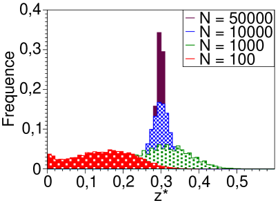
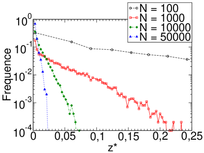
Furthermore, it can be observed that $M_{c}$ scales with $N$ as a power law with exponent lower than 1 (simulations suggest a trend $M_{c}\sim N^{\zeta}$ with $\zeta\simeq 0.4$), while nodes upstream the core that are removed by LRd and nodes downstream removed by LRu grow approximately linearly in $N$. Figures 10 show the results of simulations. The upstream part of the graph removed by LRd is indicated with the letter $U$ and the downstream part with $D$. One speculates that $U$, $D$ and $M_{c}$ at the transition point behave as

$$U\sim\alpha N\qquad D\sim\beta N\qquad M_{c}\sim N^{\zeta}\;.$$

Also the particular core structure of critical networks is affected by finite size effects. In fact, for $N=100$ it is not unusual to find core networks with more complex structures than disconnected simple loops. This also explains the behaviour of Fig.  6(d): one can speculate from the plots that the LRb core description in modular structures becomes more accurate increasing $N$, while, for smaller systems and $\gamma_{c}\leqslant\gamma\leqslant\gamma_{e}$, a single disconnected component with a more complex structure is present with more frequency.

Figure 10: Scaling with $N$ of the core $M_{c}$. Each point of simulation is the averaged result of $10^{3}$ iterations. The fit $y=ax^{b}$ with $a\simeq 0.68$ and $b\simeq-0.58$ is presented.

Appendix C Estimates of $T_{max}$

We estimate $T_{max}$ considering cores built of loop structures of lengths the first $m$ prime numbers $\{p_{1},p_{2},\ldots,p_{m}\}$, so:

$$M_{c}=\sum_{i\leqslant m}p_{i}\>,\qquad T=T_{max}=\prod_{i\leqslant m}p_{i}\;.$$

Since the $n$th prime number scales as $n\ln n$, from the above equations one has

$$M_{c} \sim \sum_{n}^{m}n\ln n\sim\frac{1}{2}m^{2}\ln m$$

$$\ln T_{max} \sim \sum_{n}^{m}\ln n+\ln\ln n\sim m\ln m\;,$$

from which

$$\ln T_{max}\sim\sqrt{M_{c}\ln M_{c}}\;.$$ (8)

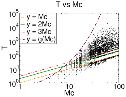
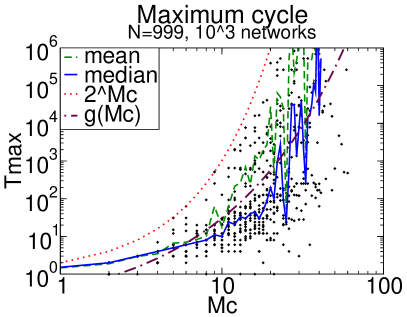
Simulated graphs show that this expression is a good upper bound for the value of $T=\textsc{lcm}\{l_{i}\}$ (Fig. 11.a). The plots indicate that these values “thicken” around multiple values of $M_{c}$. This suggests that residual graphs have a large component with dimension roughly equal to $M_{c}$ and a short loop of length 2, 3,$\ldots$
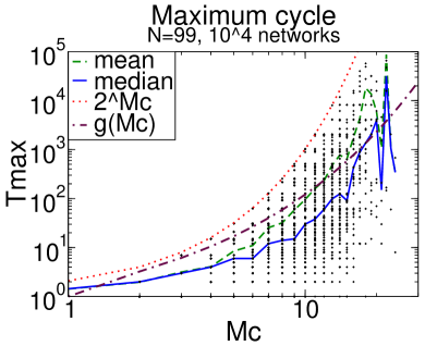
It is interesting to compare these estimates with maximum-length cycles generated by simulations of the core dynamics. Our numerical plots show the values of the maximum period $T_{max}$ emerging from reduced dynamics. In the case $N=99$ the bound set by Eq. (8) is passed several times (Fig. 11.b) because of finite size effects, but it becomes more reliable for larger systems. Figure 11.c shows that simulated values for $T_{max}$ seem to concentrate under the function $g(M_{c})\sim\exp(\sqrt{M_{c}\ln M_{c}})$. 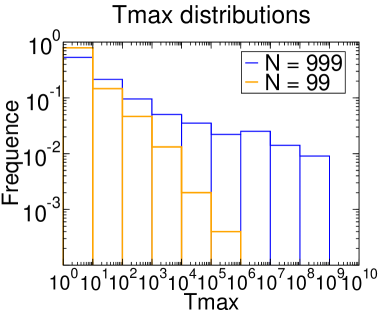Finally, Fig. 11.d shows the maximum cycle distributions for the same simulations. These are power-law like, and become broader with the system dimension. Since statistics is limited by the imposed cutoff, averages are highly biased by this computational restriction and cannot be considered reliable for large systems or much beyond the critical line.

(a)

(b)

(c)

(d)

Figure 11: Maximum cycle length for critical networks. (a) Values of $T=\mathrm{lcm}\{l_{i}\}$ vs $Mc$ for $\gamma=0.3334$, $N=10^{4}$, and $10^{4}$ different networks. $g(M_{c})\sim\exp(\sqrt{M_{c}\ln M_{c}})$. (b) and (c) are numerical simulation of the dynamics of core networks at $\gamma=0.33$ ($k=3$). The plots report the values of $T_{max}$ as a function of $M_{c}$. Dots are experimental points compared with the bound $g(M_{c})\sim\exp(\sqrt{M_{c}\ln M_{c}})$. Solid line (blue online) reports the median and the dashed one (green online) the mean. The cutoff on cycle lengths is $10^{9}$. For $N=999$ (c) this limit is passed only six times and all for $M_{c}\geqslant 48$. Estimates of central values are not calculated when data are insufficient. (d) Shape of the distributions of $T_{max}$ for $N=99$ (red online) and $N=999$ (blue online). The distributions are power-law-like and their tails are limited by the cutoff imposed ($10^{9}$).

References

- Barabasi and Oltvai (2004) A. L. Barabasi and Z. N. Oltvai, Nat. Rev. Gen. 5, 101 (2004).
- Alon (2003) U. Alon, Science 301, 1866 (2003).
- Hartwell et al. (1999) L. H. Hartwell, J. J. Hopfield, S. Leibler, and A. W. Murray, Nature 402, C47 (1999).
- Bray (2003) D. Bray, Science 301, 1864 (2003).
- Oltvai and Barabasi (2002) Z. N. Oltvai and A. L. Barabasi, Science 298 (2002).
- Lee et al. (2002) T. I. Lee et al., Science 298, 799 (2002).
- Babu et al. (2004) M. Babu, N. Luscombe, L. Aravind, M. Gerstein, and S. Teichmann, Curr. Opin. Struct. Biol. 14, 283 (2004).
- Thomas (1973) R. Thomas, J. Theor. Biol. 42, 563 (1973).
- Kauffman (1993) S. A. Kauffman, The origins of order : self-organization and selection in evolution (Oxford University Press, New York, 1993).
- Guelzim et al. (2002) N. Guelzim, S. Bottani, P. Bourgine, and F. Képès, Nat. Genet. 31, 60 (2002).
- Isalan et al. (2008) M. Isalan, C. Lemerle, K. Michalodimitrakis, C. Horn, P. Beltrao, E. Raineri, M. Garriga-Canut, and L. Serrano, Nature 17, 840 (2008).
- Kauffman (1969) S. A. Kauffman, J. Theor. Biol. 22, 437 (1969).
- Gershenson (2004) C. Gershenson, in Workshop and Tutorial Proceedings, Ninth International Conference on the Simulation and Synthesis of Living Systems (Artificial Life IX), edited by M. Bedau, P. Husbands, T. Hutton, S. Kumar, and H. Suzuki (MIT Press, 2004), pp. 160–173.
- Aldana et al. (2003) M. Aldana, S. Coppersmith, and L. P. Kadanoff, in Perspectives and Problems in Nonlinear Science, A celebratory volume in honor of Lawrence Sirovich, edited by E. Kaplan, J. E. Mardsen, and K. R. Sreenivasan (Springer, New York, 2003), Springer Applied Mathematical Science Series, pp. 23–89.
- Drossel (2007) B. Drossel, in Reviews of Nonlinear Dynamics and Complexity, edited by H. Schuster (Wiley, 2008), vol. 1.
- Ribeiro and Kauffman (2007) A. S. Ribeiro and S. A. Kauffman, J. Theor. Biol. 247, 743–755 (2007).
- Bastolla and Parisi (1997) U. Bastolla and G. Parisi, J. Theor. Biol. 187, 117 (1997).
- Seshasayee et al. (2006) A. S. N. Seshasayee, P. Bertone, G. M. Fraser, and N. M. Luscombe, Curr. Opin. Micr. 9, 511 (2006).
- Luscombe (2004) N. M. Luscombe, Nature 431, 308 (2004).
- Balaji et al. (2007) S. Balaji, M. Madan Babu, and L. Aravind, J. Mol. Biol. 372, 1108 (2007).
- Paul et al. (2006) U. Paul, V. Kaufman, and B. Drossel, Phys. Rev. E 73, 026118 (2006).
- Samuelsson and Troein (2003) B. Samuelsson and C. Troein, Phys. Rev. Lett. 90, 098701 (2003).
- Drossel (2005) B. Drossel, Phys. Rev. E 72, 016110 (2005).
- Cosentino Lagomarsino et al. (2005b) M. Cosentino Lagomarsino, P. Jona, and B. Bassetti, Phys. Rev. Lett. 95, 158701 (2005b).
- Correale et al. (2006a) L. Correale, M. Leone, A. Pagnani, M. Weigt, and R. Zecchina, J. Stat. Mech. P03002 (2006a).
- Correale et al. (2006b) L. Correale, M. Leone, A. Pagnani, M. Weigt, and R. Zecchina, Phys. Rev. Lett. 96, 018101 (2006b).
- Cosentino Lagomarsino et al. (2006) M. Cosentino Lagomarsino, P. Jona, and B. Bassetti, in Proceedings of the CMSB conference, Lecture Notes in Bioinformatics (Springer, 2006).
- Kolchin (1998) V. F. Kolchin, Random Graphs (Cambridge University Press, New York, 1998).
- Caracciolo and Sportiello (2002) S. Caracciolo and A. Sportiello, J. Phys. A: Math. Gen. 35, 7661 (2002).
- Mihaljev and Drossel (2006) T. Mihaljev and B. Drossel, Phys. Rev. E 74, 046101 (2006).
- Flyvbjerg and Kjaer (1988) H. Flyvbjerg and M. Kjaer, J. Phys. A: Math. Gen. 21, 1695 (1988).
- Bilke and Sjunnesson (2001) S. Bilke and F. Sjunnesson, Phys. Rev. E 65, 016129 (2001).
- Mézard et al. (1987) M. Mézard, G. Parisi, and M. Virasoro, Spin Glass Theory and Beyond, vol. 9 of World Scientific Lecture Notes in Physics (World Scientific Publishing Company, 1987).
- Mézard et al. (2003) M. Mézard, F. Ricci-Tersenghi, and R. Zecchina, J. Stat. Phys. 111, 505 (2003).
- Andrecut, M. and Kauffman, S. A. (2008) M. Andrecut and S. A. Kauffman, Phys. Lett. A 372, 4757-4760 (2008).
- Bauer and Golinelli (2001) M. Bauer and O. Golinelli, Eur. Phys. J. B 24, 339 (2001).
- Weigt (2002) M. Weigt, Eur. Phys. J. B 28, 369 (2002).
- Maffi (2005-2006) C. Maffi, Dynamical properties of Boolean models inspired to transcriptional regulation networks (Master degree thesis, Università degli studi di Milano, 2005-2006).
- Socolar and Kauffman (2003) J. E. S. Socolar and S. A. Kauffman, Phys. Rev. Lett. 90, 068702 (2003).
- Kaufman and Drossel (2006) V. Kaufman and B. Drossel, New J. Phys. 8, (228) (2006).
- Krawitz and Shmulevich (2007) P. Krawitz and I. Shmulevich, Phys. Rev. E 76, 036115 (2007).
- Bastolla and Parisi (1998a) U. Bastolla and G. Parisi, Physica D 115, 203 (1998a).
- Bastolla and Parisi (1998b) U. Bastolla and G. Parisi, Physica D 115, 219 (1998b).
- Kaufman et al. (2005) V. Kaufman, T. Mihaljev, and B. Drossel, Phys. Rev. E 72, 046124 (2005).
- Bassetti et al. (2007) F. Bassetti, M. Cosentino Lagomarsino, B. Bassetti, and P. Jona, Phys. Rev. E 75, 056109 (2007).