Bose-Einstein condensation in an optical lattice: A perturbation approach

Abstract

We derive closed analytical expressions for the order parameter $\Phi(x)$ and for the chemical potential $\mu$ of a Bose-Einstein Condensate loaded into a harmonically confined, one dimensional optical lattice, for sufficiently weak, repulsive or attractive interaction, and not too strong laser intensities. Our results are compared with exact numerical calculations in order to map out the range of validity of the perturbative analytical approach. We identify parameter values where the optical lattice compensates the interaction-induced nonlinearity, such that the condensate ground state coincides with a simple, single particle harmonic oscillator wave function.

I Introduction

The dynamics of Bose Einstein Condensates (BEC) in harmonically confined optical lattices is one of the key objects of cold matter research shin . While the fundamental equation which describes the mean field solution, the Gross-Pitaevski equation (GPE) Groos1 , is readily amenable to a numerical solution, explicit analytical expressions for the condensate ground state $\Phi$ and the associated chemical potential $\mu$ are scarce. Variational solutions have been proposed in perez , and quasiclassical approximations were implemented, providing several analytical results for the GPE Konotop . Eigenenergies and eigenmodes of the non-linear Schrödinger equation in a parabolically confined optical lattice can be characterized through asymptotic expansions of Mathieu functions, in the tight-binding approximation ana .

We will demonstrate in the present contribution that closed analytic results can indeed be derived, and that they permit not only qualitative but also quantitative insight into the competition between the interaction-induced nonlinearity on one hand, and the redistribution of the particles over the spatially modulated potential, on the other. Comparison with exact numerical results will finally allow us to demarcate the range of validity of our perturbation approach, with respect to parameter values employed in state of the art experiments.

II Analytical expressions

We consider the one-dimensional nonlinear GPE in a stationary optical lattice Groos1 ,

$$\left\{-\frac{\hbar^{2}}{2m}\frac{d^{2}}{dx^{2}}+\frac{1}{2}m\omega^{2}x^{2}+\lambda_{1D}\left|\Phi\right|^{2}\right.$$

$$\left.-sE_{R}\cos^{2}\left(\frac{2\pi}{d}x\right)\right\}\Phi=\mu\Phi,$$ (1)

where $\omega$ is the frequency of the confining harmonic trap Exp1 , $m$ the atomic mass, $E_{R}=$ $\frac{\hbar^{2}}{2m}(\frac{2\pi}{d})^{2}$ the recoil energy Kramer , $s\geq 0$ an adjustable parameter defined by the laser intensity, $d$ the laser wavelength, and $\lambda_{1D}$ the atom-atom interaction strength. With this one dimensional ansatz, we implicitly assume that the dynamics in the transverse direction be frozen – e.g., by sufficiently strong confinement or some other adiabaticity condition Berg . Furthermore, we imply the number of atoms per site to be large enough to justify the mean field limit Pitaevskii ; Pitaevskii2 . The normalization condition for $\Phi$ reads

$$1=\int_{-\infty}^{\infty}dx\left|\Phi\right|^{2}\,.$$ (2)

Equation (1) admits the following integral representation for $\Phi(x)$ trallero :

$$\Phi(x)=\int_{-\infty}^{\infty}G(x,x^{\prime})f(x^{\prime})dx^{\prime}\,,$$ (3)

with the Green function $G(x,x^{\prime})$ of the linear operator $L_{0}=-\frac{\hbar^{2}}{2m}d^{2}/dx^{2}+\frac{1}{2}m\omega^{2}x^{2}$, and

$$f=\left(\mu+sE_{R}\cos^{2}\left(2\pi x/d\right)-\lambda_{1D}\left|\Phi\right|^{2}\right)\Phi$$

the inhomogeneity of the differential equation $L_{0}[\Phi]=f$.

Recall that for Eq. (3) to hold, we have to impose that all involved functions tend to zero as $x\rightarrow\pm\infty$. Thus, on the basis of the general theory of Fredholm integral equations Mihling ; petrovskii ; trallero2 , the harmonic oscillator functions $\{\varphi_{n}\}$ represent a complete basis set which span the Hilbert space of the integral equation (3). Using the spectral representation of $G(x,x^{\prime})$, we can rewrite the order parameter $\Phi$ as

$$\Phi=\sum_{n=0}^{\infty}\varphi_{n}(\frac{x}{l_{o}})C_{n}(\mu)\,,$$ (4)

where $l_{o}=\sqrt{\hbar/m\omega}$ is the harmonic oscillator wavelength. Inserting (4) into (3), the vector coefficient $\mathbf{C}(\mu)=\{C_{n}(\mu)\}_{n=0}^{\infty}$ is restricted to obey the relation Mikhlin

$$\left[\mathbf{\Delta}(\mu)+\Lambda\mathbf{C}^{\tau}\mathbf{\cdot T}\cdot\mathbf{C-}V_{o}\mathbf{P}\right]\mathbf{C}=0\,,$$ (5)

with $\mathbf{C}^{\tau}$ the transpose of the vector $\mathbf{C}$. $T_{plmn}$ and $P_{km}$ are fourth and second rank tensors, respectively, and defined in Appendices A and B. Furthermore, $V_{o}=sE_{R}/\hbar\omega$, $\Lambda=\lambda_{1D}/l_{o}\hbar\omega$, and

$$\mathbf{\Delta}_{nm}=\left(n+\frac{1}{2}-\frac{\mu}{\hbar\omega}\right)\delta_{nm}\,.$$ (6)

II.1 Chemical potential

We tackle the problem under the assumption that the atom-atom interaction, the nonlinear term $\lambda\left|\Phi\right|^{2}$, and the optical lattice potential can be considered as perturbations with respect to the trap potential $m\omega^{2}x^{2}/2$. In this case, the dimensionless chemical potential $\mu/\hbar\omega$ and the vector $\mathbf{C}$ in Eq. (5) can be expanded in series,

$$\mathbf{C} = \mathbf{C}^{(0)}+\mathbf{C}^{(1)}+\mathbf{C}^{(2)}+\ldots\,,$$ (7)

$$\frac{\mu}{\hbar\omega} = \mu^{(0)}+\mu^{(1)}+\mu^{(2)}+\ldots\,,$$ (8)

where the quantities $\mathbf{C}^{(i)}$ and $\mu^{(i)}$ are understood to be of the same order in $\Lambda$ and $V_{o}$. Expansion of Eq. (5) to second order in $\Lambda$ and $V_{o}$ leads, after lengthy but straightforward manipulation, the following expression for the system’s ground state energy:

$$\frac{\mu}{\hbar\omega} = \frac{1}{2}+\Lambda T_{0000}-V_{o}P_{00}-3\Lambda^{2}\sum_{m=1}^{\infty}\frac{\left|T_{0002m}\right|^{2}}{2m}+$$ (9)

$$4\Lambda V_{o}\sum_{m=1}^{\infty}\frac{T_{0002m}P_{02m}}{2m}-V_{0}^{2}\sum_{m=1}^{\infty}\frac{\left|P_{02m}\right|^{2}}{2m}\,.$$

Using the properties of $T_{plmn}$ and $P_{kp}$ given in the Appendices A and B we obtain

$$\frac{\mu}{\hbar\omega} = \frac{1}{2}+\frac{\Lambda}{\sqrt{2\pi}}-\frac{V_{o}}{2}\left[1+\exp\left(-\alpha^{2}\right)\right]+$$ (10)

$$\frac{\Lambda V_{o}}{\sqrt{2\pi}}\exp\left(-\alpha^{2}\right)\sum_{m=1}^{\infty}\frac{\alpha^{2m}}{m2^{m}m!}-$$

$$\frac{3\Lambda^{2}}{2\pi}\sum_{m=1}^{\infty}\frac{(2m-1)!}{2^{4m}(m!)^{2}}-$$

$$\frac{V_{o}^{2}}{4}\exp\left(-2\alpha^{2}\right)\sum_{m=1}^{\infty}\frac{2^{2m}\alpha^{4m}}{2m(2m)!}\,,$$

with $\alpha=2\pi l_{o}/d$ the ratio of trap to laser wavelength. Finally, the series in (10) can be summed up with the help of Eqs. (30-33) in Appendix C, and we obtain for the chemical potential, at second order in $\Lambda$ and $V_{o}$:

$$\frac{\mu}{\hbar\omega} = \frac{\Lambda}{\sqrt{2\pi}}+\frac{1-V_{o}}{2}-\frac{V_{o}}{2}\exp\left(-\alpha^{2}\right)$$ (11)

$$+\frac{\Lambda V_{o}}{\sqrt{2\pi}}\exp\left(-\alpha^{2}\right)\left\{Ei(\frac{\alpha}{2})-\mathcal{C}-\ln\frac{\alpha}{2}\right\}$$

$$-0.033106\times\Lambda^{2}$$

$$-\frac{V_{o}^{2}}{4}\exp\left(-2\alpha^{2}\right)\left\{Chi(2\alpha)-\mathcal{C}-\ln 2\alpha\right\}.$$

II.2 Order parameter

Following the same procedure as above, $\mathbf{C}$ and thus (through (4)) the normalized order parameter $\Phi$ can be expressed, at first order in $\Lambda$ and $V_{o}$, as

$$\Phi=\varphi_{{}_{0}}(\frac{x}{l_{o}})-\sum_{m=1}^{\infty}\frac{\Lambda T_{0002m}-V_{o}P_{02m}}{2m}\varphi_{2m}(\frac{x}{l_{o}})\,.$$ (12)

With the expressions derived in the Appendices A and B for the matrix elements $T_{0002m}$ and $P_{02m}$, this can be rewritten as

$$\Phi = \varphi_{{}_{0}}(\frac{x}{l_{o}})+\sum_{m=1}^{\infty}\frac{\left(-1\right)^{m+1}}{2m}\left\{\frac{\Lambda\sqrt{\left(2m\right)!}}{\sqrt{2\pi}2^{2m}m!}-\right.$$ (13)

$$\left.\frac{V_{o}2^{m-1}}{\sqrt{\left(2m\right)!}}\alpha^{2m}\exp\left(-\alpha^{2}\right)\right\}\varphi_{2m}(\frac{x}{l_{o}})\,.$$

Since, according to Eqs. (34-37) of Appendix C,

$$F\left(z,\alpha\right)=\frac{\exp\left(-\alpha^{2}\right)}{\sqrt{\pi^{1/2}}}\sum_{m=1}^{\infty}\frac{\left(-1\right)^{m}2^{m-1}}{2m\sqrt{\left(2m\right)!}}\alpha^{2m}\varphi_{2m}(z)$$

equals

$$F\left(z,\alpha\right) = \frac{1}{\sqrt{l_{o}\pi^{1/2}}}\exp\left(-\alpha^{2}\right)\exp\left(-z^{2}/2\right)\times$$

$$\int\nolimits_{0}^{\alpha}\left[\exp(y^{2})\cos\left(2yz\right)-1\right]\frac{dy}{2y}\,,$$

and, moreover, with (LABEL:f-41),

$$G\left(z\right)=\sum_{m=1}^{\infty}\frac{\left(-1\right)^{m+1}\sqrt{(2m)!}}{2m2^{2m}\sqrt{2\pi}m!}\varphi_{2m}(z)$$

can be condensed into

$$G\left(z\right)=\frac{\exp\left(-z^{2}/2\right)}{\sqrt{2\pi}\sqrt{l_{o}\pi^{1/2}}}\int\nolimits_{1}^{\sqrt{2}/2}\frac{\exp\left(-\frac{z^{2}}{y^{2}}\left(1-y^{2}\right)\right)-y}{1-y^{2}}dy\,,$$

we obtain the following closed expression for the order parameter:

$$\Phi=\varphi_{{}_{0}}(\frac{x}{l_{o}})+\frac{\Lambda}{\sqrt{l_{o}}}G\left(\frac{x}{l_{o}}\right)+\frac{V_{o}}{\sqrt{l_{o}}}F\left(\frac{x}{l_{o}},\alpha\right)\,.$$ (14)

II.3 Numerical Solution

For a numerical solution of Eq. (1), we subdivide the dimensionless coordinate $z=x/l_{o}$, $z\in[-L;L]$, such that $z_{i}=(-L/2+(i-1))\delta$, $i=1,\ldots,L+1$, with a grid size $\delta$. For $\delta\ll d/l_{o}$, a three-point approximation with uniform spacing allows to rewrite the second derivative and the differential equation (1) as difference equations:

$$\left.\left(\frac{z_{i}^{2}}{2}+\Lambda\left|\overline{\phi_{i}}\right|^{2}-V_{o}\cos^{2}\frac{{2\pi{l}_{o}z_{i}}}{d}+\frac{1}{\delta^{2}}\right)\overline{\phi_{i}}\right.$$

$$\left.-\frac{\overline{\phi_{i-1}}}{2\delta^{2}}-\frac{\overline{\phi_{i+1}}}{2\delta^{2}}=\frac{\mu}{\hbar\omega}\overline{\phi_{i}}\right.\,,$$ (15)

where $\overline{\phi_{i}}=\sqrt{{{l}_{o}}}\Phi(z_{i})$ is the local, normalized order parameter which abides by the boundary conditions $\overline{\phi_{0}}=\overline{\phi_{L+2}}=0$.

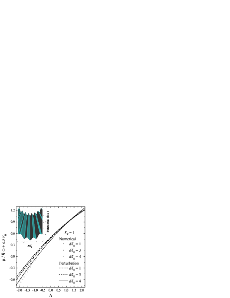
Figure 1: (Color online) Variation of the chemical potential $\mu/\hbar\omega+V_{o}/2$ as a function of the dimensionless self-interaction parameter $\Lambda$. Solid, dashed, and dash-dotted lines represent the analytical results for $d/l_{o}=$ 1, 2 and 3, respectively. Symbols correspond to the numerical solution of Eq. (1). The strength of the periodic potential was set to $V_{o}=sE_{R}/\hbar\omega=$ 1. Inset: Confining potential $U=\frac{1}{2}m\omega^{2}x^{2}-sE_{R}\cos^{2}\left(\frac{2\pi}{d}x\right)$ for $2<d/l_{o}<4$.

Equation (15) defines a tri-diagonal eigenvalue problem with the normalization condition $\sum_{i}|\overline{\phi_{i}}|^{2}\delta=1$ or, equivalently, $\sum_{i}|\tilde{\phi}_{i}|^{2}=1$, where $\tilde{\phi}_{i}=\sqrt{\delta}\bar{\phi}_{i}$. Since the resulting matrix (15) involves the non-linear term $\left|\overline{\phi_{i}}\right|^{2}$, an iterative procedure is needed for a self-consistent solution. To avoid numerical instabilities trallero2 ; Pu , we inserted the iterative wave function

$$F_{i}^{(k)}=\sqrt{(1-\varepsilon)\left|\tilde{\phi}_{i}^{(k-1)}\right|^{2}+\varepsilon\left|\tilde{\phi}_{i}^{(k)}\right|^{2}}$$ (16)

in (15), at each new iteration $k$, with $\varepsilon\in[0;1]$, and starting condition $F_{i}^{(0)}=\tilde{\phi}_{i}^{(0)}$. This procedure was repeated until $\left|\tilde{\phi}_{i}^{(k)}-\tilde{\phi}_{i}^{(k-1)}\right|<\delta_{\phi}$ and $|(\mu^{(k)}-\mu^{(k-1)})/\hbar\omega|<\delta_{\mu}$, where $\delta_{\phi}$ and $\delta_{\mu}$ are the desired accuracies for the order parameter and the chemical potential, respectively. Our iterative solutions then converge to a relative uncertainty of $10^{-4}$ for $\mu/\hbar\omega$ and the normalized order parameter.

III Results

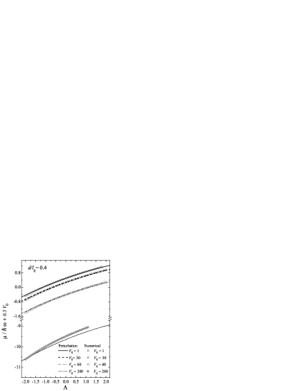
Figure 2: Same as in Fig. 1, for $V_{o}=$ 1 (solid line), 30 (dashed line), 60 (dash-dotted line), and 200 (dotted line). Symbols represent the analytical results. The laser wavelength was set to $d/l_{o}=$0.4.

Figure 3: Normalized order parameter $\sqrt{l_{0}}\Phi(x/l_{0})$ for the dimensionless self-interaction values: (a) $\Lambda=$0, (b) -0.5, (c) -1.0, and (d) -1.5. $V_{o}=$ 1 and $d/l_{o}=$1. Solid line: Closed solution according to Eq. (14). Open circles: Numerical result.

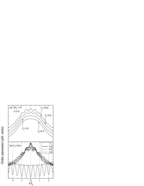
Figure 4: Order parameter $\Phi(x/l_{0})$ for $d/l_{o}=$ 1. (a) $\Lambda$ =2, $V_{o}=sE_{R}/\hbar\omega=$ 0.5, 1, 5, and 10. (b) $V_{o}=$ 10, $\Lambda$ =-2, 0, 2. Symbols represent the numerical solution. For the sake of comparison, $U$ (see caption Fig. 1) and the harmonic oscillator potential are shown by solid and dashed lines, respectively.

Figure 1 displays the variation of the chemical potential, $\mu/\hbar\omega+0.5V_{o}$, as a function of the dimensionless atom-atom interaction $\Lambda$. The analytical solution (10) is represented by solid, dashed, and dash-dotted lines, while symbols represent the numerical solutions of Eq. (1). The inset illustrates the confining potential $U=m\omega^{2}x^{2}/2-sE_{R}\cos^{2}\left(2\pi x/d\right)$, as a function of $x/l_{o},$ for $V_{o}=1$ and $2<d/l_{o}<4$. In our calculation of $\mu$, we fixed $V_{o}=1$ and checked the variation of the perturbative solution as compared to the numerical one, for several values $d/l_{o}=1,3$ and $4$ of the normalized wavelength. For $\Lambda<0$ the relative error between the numerical solution and Eq. (11) increases as $d/l_{o}$ increases, while for $\Lambda>0$ the worst comparison is obtained at $d/l_{o}=1$. In the case of repulsive interaction, numerical and perturbative calculation exhibit small variations with $d/l_{o}$. In general, Eq. (11) describes the values of the chemical potential better for repulsive than for attractive interaction. This can be understood with the following argument: In trallero ; trallero2 it was shown shown that, at $V_{o}=0$, perturbation theory matches the numerical solution very well in the interval $-2<\Lambda<2$. When the optical lattice is switched on ($V_{o}\neq 0$), we can argue that an effective renormalization of the non-linear parameter takes place. Since Eq. (11) includes a negative quadratic term in $V_{o}$, we expect that the effective range of $\Lambda$ where perturbation theory is applicable will shift to $\Lambda>-2$, i.e., more repulsive or less attractive atom-atom interactions. Naturally, the behavior of the chemical potential with $d/l_{o}$ limits this simple description.

In Fig. 2, we plot the dependence of $\mu(\Lambda)/\hbar\omega+0.5V$ on $\Lambda$, for several values of the strength of the periodic potential $V_{o}$. In the calculation we took $d/l_{o}=0.4$. The figure shows perfect agreement of Eq. (11) with the numerical result for $V_{o}$ ranging between $1$ and $60$, while, at $V_{o}=200$, we observe large discrepancies.

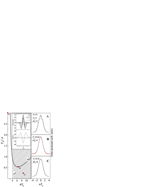
Figure 5: (Color online) Quenching of the non-linear repulsive interaction. Left panel: Region $\mathcal{H}$ is defined by the condition (17). The curve $\mathcal{D}$ is defined by Eq. (17), at $x=0$. Right panel: Order parameter calculated for those parameter values identified by A, B, and C on the left. Solid lines represent $\Phi$ as derived from Eq. (14), while open circles indicate the exact numerical solution. Dashed lines correspond to the harmonic oscillator wave function.

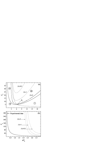
Figure 6: (a) Range of validity of Eq. (11) in the $V_{o}$-$d/l_{o}$-plane. The functions Linear, Mixed and Quadratic (see text) are represented by dashed, dotted and solid lines, respectively. $z_{c}=[(V_{o})_{c},(d/lo)_{c}$ ] is defined by equality between Linear and Quadratic. (b) Zoom into the region of large values of $V_{o}$. The circle locates the parameter values employed in the experiments reported in Ott .

Figure 3 displays the normalized order parameter, $\Phi(x/l_{0})\sqrt{l_{0}},$ for four values of $\Lambda=0,-0.5,-1.0$, and $-1.5$, and fixed $V_{o}=10$, $d/l_{o}=1$. In general, we obtain a remarkably good agreement between the analytical prediction (14) and the numerical result, for all considered (attractive) values of the dimensionless interaction parameter $\Lambda$, and witness the interplay between the optical lattice and harmonic oscillator potential: The harmonic oscillator ground state $\varphi_{{}_{0}}$ is modulated by an oscillatory behavior, induced by the optical lattice potential. We further note that the wave function gets more localized, and the maximum of $\Phi(x/l_{0})$ increases, as the non-linear potential becomes more attractive. Panel (a) of Fig. 4 shows the variation of $\Phi(x/l_{0})\sqrt{l_{0}}$ with the strength of the periodic potential $V_{o}$, for the repulsive case $\Lambda=2$. As $V_{o}$ increases from 0.5 to 10, the lattice-induced density oscillations manifest with increasing amplitude. A comparison between attractive and repulsive interactions, for $V_{o}=10$, is given by panel (b) of Fig. 4: Since $d/l_{o}=1$ in Figs. 3 and 4, the wave function $\Phi(x/l_{0})$ exhibits oscillations at $x/l_{0}\approx n/2$ ($n=\pm 1,\pm 2,\ldots$), which are quenched because of the asymptotic decay $\propto$ $\exp\left(-x^{2}/2l_{o}^{2}\right)$ of the oscillator wave functions. These oscillations are illustrated in Fig. 4(b), where the solid line represents the potential $U$ (see inset of Fig. 1), along with the wavefunction $\Phi$ for the same values of $V_{o}$ and $d/l_{o}$. The positions of the observed maxima (minima) in the order parameter correspond to the minima (maxima) of the resulting effective potential $U$.

The extrema of $\Phi$ exhibit different behavior depending on the non-linear interaction $\Lambda$. As the condensate becomes effectively less confined for increasing repulsive interaction, the amplitudes of the maxima and minima of $\Phi$ are enhanced. From the physical point of view it is clear that a strongly attractive interaction (in the figure: $\Lambda=-2$) should flatten the lattice-induced oscillations of the condensate. In panel (b) we compare the evolution of the order parameter from attractive to repulsive interaction. We note that, as $\Lambda$ increases, the condensate spreads, i.e., the wave function delocalizes, while its maximum decreases. The analytical solution (14) is less accurate at $x=0$ and $\Lambda=-2$ (with an error less than $5\%$), in agreement with the results of Fig. 1 and the anticipated range of validity of perturbation theory. Nevertheless, in this particular case the observed agreement with the exact solution is quite remarkable at $x\neq 0$, and shows that the closed analytical expressions derived here allow a fair representation of the BEC wave function in an optical lattice. Almost no differences can be observed on the scale of the figure between numerical and analytical solutions for $\Lambda=2$.

III.1 Quenching of the non-linear interaction

Since the repulsive atom-atom interaction and the optical lattice potential have opposite signs, the set of parameters ($\lambda_{1D}$, $\omega$, $d$, $sE_{R}$) can be chosen such as to minimize the effect of the non-linearity. To study this quenching effect, in the validity range of our perturbation approach, we consider the order parameter given by Eq. (14). In the inset of the left panel of Fig. 5, we monitor the dependence of $G(x/l_{o})$ and $F\left(x/l_{o},\alpha\right)$ on $x/l_{o}$. While the function $G$ is universal, $F$ shows a strong dependence on the parameter $d/l_{o}$. Moreover, for $d/l_{o}=4$ the contribution of $F$ to the order parameter, induced by the optical lattice, resembles the function $G$, though with opposite sign. If we impose the condition

$$\Lambda G(x/l_{o})+V_{o}F\left(x/l_{o},\alpha\right)\rightarrow 0\,,$$ (17)

then $\Phi$ can be solely described by the harmonic oscillator wave function $\varphi_{{}_{0}}$. The range of values of $\Lambda/V_{o}$, $d/l_{o}$, and $x/l_{o}$ that satisfy (17) is represented by the hatched region $\mathcal{H}$ in Fig. 5. At $x=0$, Eq. (17) defines the curve $\mathcal{D}$ shown in the figure. We have noted that at $x=0$ the functions $G$ and $F$ reach their minimum and maximum values, respectively. In the right panel of the figure we compare the harmonic oscillator wave function $\varphi_{{}_{0}}$ with the order parameter as predicted by (14). We chose three different points $A$, $B$, and $C$ in the parameter space of the left panel for this comparison: Indeed, $A$ does not fulfill the condition (17), and, consequently, $\Phi$ does not match $\varphi_{{}_{0}}$. The case $C$ belongs to region $\mathcal{H}$, but not to the curve $\mathcal{D}$. Hence, we observe a small discrepancy between both functions, mainly at $x=0$. Case $B$, which sits right on top of the curve $\mathcal{D}$, yields a perfect match between harmonic oscillator wave function and order parameter. Exact numerical solution of the GPE (1) with the parameters defined by $B$ corroborates this result, as indicated by the open circles in the figure.

III.2 Validity of the perturbation approach

For a vanishing lattice, $V_{o}=0$, our closed analytical solution for the chemical potential and its comparison with the numerical solution provides universal criteria for its range of validity: in the interval $\left|\Lambda\right|<2$, we derive an accuracy better than $97\%$ trallero ; trallero2 for Eq. (11). For nontrivial values of the lattice strength, two more independent parameters, $V_{o}$ and $d/l_{o}$ come into game. A necessary condition for the validity of the perturbative results requires that the functions $\mathit{Linear}=V_{o}\exp\left(-\alpha^{2}\right)/2$, $\mathit{Mixed}=\Lambda V_{o}\exp\left(-\alpha^{2}\right)\left\{Ei(\frac{\alpha}{2})-\mathcal{C}-\ln\frac{\alpha}{2}\right\}/\sqrt{2\pi}$, and $\mathit{Quadratic}=V_{o}^{2}\exp\left(-2\alpha^{2}\right)\left\{Chi(2\alpha)-\mathcal{C}-\ln 2\alpha\right\}/4$, that contribute to Eq. (11), simultaneously be smaller than one. This criterion allows to confine the range of validity of our analytical results in a 2D map spanned by $V_{o}$ and $d/l_{o}$, as displayed in Figs. 6(a) and (b). There the $\mathit{Mixed}$ contribution to (11) is plotted for three different values of $\left|\Lambda\right|=0.5$, $1$, and $2$. Fig. 6(a) thus defines different $V_{o}$ vs. $d/l_{o}$ regions where Eq. (11) can be trusted: In region I, the quadratic term in $V_{o}$ is less important than the linear one, while, in region II, we need to make one more distinction, depending on the $d/l_{o}$ values. For example, if $d/l_{o}<(d/l_{o})_{c}$, we have that $\mathit{Quadratic}$ represents the main contribution to $\mu$, and vice versa if $d/l_{o}>(d/l_{o})_{c}$, where $\mathit{Linear>Quadratic}$. A similar analysis applies in regions III and IV, with respect to the relative contributions of $\mathit{Linear}$ and $\mathit{Mixed}$.

Finally, let us note that experimental data as reported in Ott on ⁸⁷Rb condensates were obtained for $V_{o}=275$ and $d/l_{o}=0.19$. This working point is indicated by a solid circle in Fig. 6(b), and shows that our perturbative method is applicable in the experimental parameter range.

IV Conclusions

We provided closed analytical expressions for the chemical potential and the particle density of the GPE ground state in an optical lattice. These solutions were obtained by a perturbative expansion in the lattice strength and in the (attractive or repulsive) atom-atom interaction, with a well-controlled range of validity in the associated parameter space.

Interestingly, the interaction-induced non-linearity may be quenched by the presence of the lattice. Under certain conditions (see left panel of Fig. 5), we predict that the particle density of the repulsively interacting system is given by $\Phi(x,t)=\exp(i\mu[\Lambda,V_{o},d/l_{0}]t/\hslash)\varphi_{{}_{0}}(x/l_{0})$.

The solutions derived here can serve as a useful tool to study a weakly interacting BEC in a not too deep 1D optical lattice. On this basis, it is possible to develop a unified and comprehensive picture of Bogoliubov equations, the time-dependent GPE and of collective excitations (a subject under investigation). The model here developed can be generalized to two and three dimensions, and also for two component BECs.

Appendix A Tensor $\mathbf{T}$

Using the harmonic oscillator wave function

$$\varphi_{n}(x)=\left(\frac{1}{\pi^{1/2}2^{n}n!l_{0}}\right)^{1/2}\exp\left(-\frac{x^{2}}{2l_{0}{}^{2}}\right)H_{n}\left(\frac{x}{l_{0}}\right),$$ (18)

with $H_{n}(z)$ the Hermite polynomials, the matrix elements $T_{plmn}$ are defined by

$$T_{plmn} = \frac{1}{\pi\sqrt{2^{n+m+l+p}n!m!l!p!}}\times$$

$$\int_{-\infty}^{\infty}\exp(-2z^{2})H_{n}(z)H_{m}(z)H_{l}(z)H_{p}(z)dz\,.$$

It is possible to perform the above integral, and we get trallero2 ; lord

$$T_{p,l,n,m} = \frac{(-1)^{M-m-p}2^{M-\frac{1}{2}}}{\pi\sqrt{2^{n+m+l+p}n!m!l!p!}}\times$$ (22)

$$\frac{\Gamma(M-l+\frac{1}{2})\Gamma(M-n+\frac{1}{2})}{\Gamma(M-n-l+\frac{1}{2})}\times$$

$$\text{ }_{\text{3}}F_{\text{2}}\left(\begin{array}[]{cc}-m,\text{ \ }-p,&-M+n+l+\frac{1}{2};\\ -M+l+\frac{1}{2},&-M+n+\frac{1}{2};\end{array}1\right)\,,$$

with $\Gamma(z)$ the gamma function, ${}_{\text{3}}F_{\text{2}}\left(\begin{array}[]{ccc}\alpha_{1},&\alpha_{2},&\alpha_{3};\\ &\beta_{1},&\beta_{2};\end{array}1\right)$ the generalized hypergeometric function Gradshteyn80 , and $2M=p+l+m+n$. Consequently, we arrive at the following useful relations: i) $T_{plmn}=0$, if $n+m+l+p$ is an odd number, ii), for $m=0$ Gradshteyn80 ,

$$T_{pln0}=\frac{2^{s-1}}{\pi^{2}}\frac{\Gamma(s-l)\Gamma(s-p)\Gamma(s-n)}{\sqrt{2^{n+l+p}l!p!n!}}\,,$$ (24)

and, iii), for $p=l=n=0$,

$$T_{0002m}=\left(-1\right)^{m}\frac{\sqrt{\left(2m\right)!}}{\sqrt{2\pi}2^{2m}m!}\,.$$ (25)

Appendix B Tensor $\mathbf{P}$

The contribution of the optical lattice is represented by the two dimensional matrix elements $P_{kp}$ given by

$$P_{kp} = \frac{1}{\sqrt{\pi 2^{k+p}k!p!}}\int_{-\infty}^{\infty}\left[\cos^{2}(\frac{2\pi l_{o}}{d}z)\right.\times$$ (26)

$$\left.H_{k}(z)H_{p}(z)\exp(-z^{2})\right]dz.$$

For $p=k+2m$ this integral is equal to Gradshteyn80

$$P_{kp} = \frac{1}{2^{m+1}}\sqrt{\frac{k!}{\left(k+2m\right)!}}\left\{\delta_{m,0}+\right.$$ (27)

$$\left.\left(-1\right)^{m}b^{2m}\exp\left(-b^{2}/4\right)L_{k}^{2m}\left(\frac{b^{2}}{2}\right)\right\}\,,$$

where $b=4\pi l_{o}/d$ and $L_{k}^{t}\left(x\right)$ are the Laguerre polynomials. The symmetry of the Hermite polynomials imposes that $P_{kp}=0$ if $p=k+2m+1$. Using (27) the following relations hold: i) For $k=p=0$,

$$P_{00}=\frac{1}{2}+\frac{1}{2}\exp\left[-\left(\frac{2\pi l_{o}}{d}\right)^{2}\right]\,,$$ (28)

and, ii), for $k=0$ and $p=2m$,

$$P_{02m}=\frac{\left(-2\right)^{m}}{2\sqrt{(2m)!}}\left(\frac{2\pi l_{o}}{d}\right)^{2m}\exp\left(-\left(\frac{2\pi l_{o}}{d}\right)^{2}\right)\,.$$ (29)

Appendix C Series

We can sum up the series

$$F1=\frac{3}{2\pi}\sum_{m=1}^{\infty}\frac{(2m-1)!}{2^{4m}(m!)^{2}}$$ (30)

noting that

$$\sum_{m=1}^{\infty}\frac{(2m-1)!}{2^{3m}(m!)^{2}(x^{2}+1)^{m}}=-\ln\left(\frac{1}{2}\sqrt{\frac{2x^{2}+1}{2(x^{2}+1)}}+\frac{1}{2}\right)^{2}\,.$$ (31)

Hence, $F1=0.033106$.

Furthermore, we have the series Gradshteyn80

$$\sum_{m=1}^{\infty}\frac{1}{m2^{m}m!}\alpha^{2m}=Ei(\frac{\alpha}{2})-\mathcal{C}-\ln\frac{\alpha}{2}\,,$$ (32)

and Abramowitz

$$\sum_{m=1}^{\infty}\frac{2^{2m}}{2m(2m)!}\alpha^{4m}=Chi(2\alpha)-\mathcal{C}-\ln 2\alpha\,,$$ (33)

where $Ei(x)$ is the exponential integral, $Chi(x)$ is the cosine hyperbolic integral, and $\mathcal{C}$ is Euler’s constant.

For the summation of the first part of the series in (13), we note that

$$F2(z,\alpha) = \sum_{m=1}^{\infty}\frac{\left(-2\right)^{m}\alpha^{2m}}{2\sqrt{(2m)!}}\varphi_{2m}(z)$$ (34)

$$= \frac{\exp(-z^{2}/2)}{2\sqrt{l_{0}\pi^{1/2}}}\left(\exp\alpha^{2}\cos 2\alpha z-1\right)\,.$$

The series

$$G1(z,\alpha)=\frac{1}{2}\sum_{m=1}^{\infty}\frac{\left(-2\right)^{m}\alpha^{2m}}{2m\sqrt{(2m)!}}\varphi_{2m}(z)$$ (35)

is related to the function $F2(z,\alpha)$ through the differential equation

$$\frac{dG1(z,\alpha)}{d\alpha}=\frac{F2(z,\alpha)}{\alpha}\,.$$ (36)

The solution of (36) is given by

$$G1(z,\alpha) = \frac{1}{2\sqrt{l_{0}\pi^{1/2}}}\exp\left(-\frac{z^{2}}{2}\right)$$ (37)

$$\int_{0}^{\alpha}\frac{1}{y}\left[\exp(y^{2})\cos\left(2yz\right)-1\right]dy\,.$$

To perform the sum of the first series in (13), we use that

$$F3(z,c) = \frac{1}{\sqrt{l_{0}\pi^{1/2}}}\left[c\exp(-c^{2}z^{2}+\frac{z^{2}}{2})-\exp\left(-\frac{z^{2}}{2}\right)\right]$$

$$= \sum_{m=1}^{\infty}\frac{\left(-1\right)^{m}\sqrt{\left(2m\right)!}}{2^{m}m!}\left(1-\frac{1}{c^{2}}\right)^{m}\varphi_{2m}(z)\,.$$

Now the series

$$g(z,c)=\sum_{m=1}^{\infty}\frac{\left(-1\right)^{m+1}\sqrt{\left(2m\right)!}}{m2^{m}m!}\left(1-\frac{1}{c^{2}}\right)^{m}\varphi_{2m}z)$$ (39)

is related to the function $F3(z,c)$ through the equation

$$\frac{dg}{d\beta}=\frac{2\beta}{\left(1-\beta^{2}\right)}F3\,,$$ (40)

with $\beta=1/c.$ The differential equation (40) admits the solution

$$g(z,c)=\frac{2\exp\left(-\frac{z^{2}}{2}\right)}{\sqrt{l_{0}\pi^{1/2}}}\int\nolimits_{1}^{1/c}\frac{\exp\left(-\frac{z^{2}}{y^{2}}\left(1-y^{2}\right)\right)-y}{1-y^{2}}dy\,.$$ (41)

References

• (1) Th. Anker, M. Albiez, R. Gati, S. Hunsmann, B. Eiermann, A. Trombettoni, and M. K. Oberthaler, Phys. Rev. Lett. 94, 020403 (2005); Y. Shin, G.-B. Jo, M. Saba, T. A. Pasquini, W. Ketterle, and D. E. Pritchard, Phys. Rev. Lett. 95, 170402 (2005); A. V. Ponomarev, J. Madroñero, A. R. Kolovsky, and A. Buchleitner, Phys. Rev. Lett. 96, 050404 (2006); K. Winkler, G. Thalhammer, F. Lang, R. Grimm, J. H. Denschlag, A. J. Daley, A. Kantian, H. P. Büchler, and P. Zoller, Nature 441, 853 (2006); T. Roscilde and J. I. Cirac, Phys. Rev. Lett. 98, 190402 (2007); J. Brand and A.R. Kolovsky, Eur. Phys. J. D 41, 331 (2007).
• (2) E. P. Gross, Nuovo Cimento 20, 454 (1961); L. P. Pitaevskii, Zh. Eksp. Teor. Fiz. 40, 646 (1961) [Sov. Phys. JETP 13, 451 (1961)].
• (3) V. M. Pérez-García, H. Michinel, J. I. Cirac, M. Lewenstein, and P. Zoller, Phys. Rev. Lett. 77, 5320 (1996); ibid, Phys. Rev. A 56, 1424 (1997); V. I. Yukalov, E. P. Yukalova, and V. S. Bagnato, Laser Phys. 12, 1325 (2002); ibid, Phys. Rev. A 66, 025602 (2002);
• (4) V. Konotop and P. Kevrekidis, Phys. Rev. Lett. 91, 230402 (2003); T. Hyouguchi, R. Seto, M. Ueda, and S. Adachi, Ann. of Phys. 312, 177 (2004); D. Witthaut, H. J. Korsch, J. Phys. A: Math. Gen. 39, 14687 (2006)..
• (5) A. M. Rey, G. Pupillo, Ch. W. Clark, and C. J. Williams, Phys. Rew. A 72, 033616 (2005).
• (6) M. H. Anderson, J. R. Ensher, M. R. Matthews, C. E. Wieman, E. A Cornell, Science 269, 198 (1995).
• (7) M. Krämer, L. Pitaevskii, and S. Stringari, Phys. Rev. Lett. 88, 180404 (2002).
• (8) K. Berg-Sørensen and K. Mølmer, Phys. Rev. A 58, 1480 (1998); S. Burger, F. S. Cataliotti, C. Fort, F. Minardi, M. Inguscio, M. L. Chiofalo, and M. P. Tosi, Phys. Rev. Lett. 86, 4447 (2001).
• (9) F. Dalfovo, S. Giorgini, L. P. Pitaevskii, and S. Stringari, Rev. Mod. Phys. 71, 463 (1999).
• (10) L. Pezzè, L. Pitaevskii, A. Smerzi, Stringari, G. Modugno, E. de Mirandes, F. Ferlaino, H. Ott, G. Roati, and M. Inguscio, Phys. Rev. Lett. 93, 120401 (2004).
• (11) C. Trallero-Giner, J. Drake, V. López-Richard, C. Trallero-Herrero, Joseph L. Birman, Physics Letters A 354, 115 (2006).
• (12) S. G. Mikhlin and K. L. Prössdorf, Approximate Methods for Solutions of Differential and Integral Equations (American Elsevier Publ. Co., NY, 1967).
• (13) I. G. Petrovskii, Lectures on the Theory of Integral Equations (Graylock Press, Rochester, 1957).
• (14) C. Trallero-Giner, J. Drake, V. López-Richard, C. Trallero-Herrero, Joseph L. Birman, Physica D, 237, 2342 (2008).
• (15) From general arguments it is possible to show that the expansion (4) converges in the mean, i.e. $\lim\limits_{N\rightarrow\infty}\int\limits_{0}^{\infty}\left|\Phi-\sum\limits_{n=0}^{N}\varphi_{n}(x/l_{o})C_{n}(\mu)\right|^{2}dx=0$ (see S. G. Mikhlin, Variational Methods in Mathematical Physics (Pergamon Press, 1964)). This allows to manipulate the integral in (3) and the series (4) such as to derive the relation (5).
• (16) H. Pu and N. P. Bigelow, Phys. Rev. Lett. 80, 1130 (1998).
• (17) H. Ott, E. de Mirandes, F. Ferlaino, G. Roati, G. Modugno, and M. Inguscio, Phys Rev. Lett. 92, 160601 (2004).
• (18) R. D. Lord, J. London Math. Soc. 24, 101 (1949).
• (19) I. S. Gradshteyn and I. M. Ryzhik, Tables of Integrals, Series and Products (Academic, NY, 1980).
• (20) Handbook of Mathematical Functions, edited by M. Abramowitz and I. Stegun (Dover, NY, 1972)