Stability of Maximum likelihood based clustering methods: exploring the backbone of classifications
Abstract
Components of complex systems are often classified according to the way they interact with each other. In graph theory such groups are known as clusters or communities. Many different techniques have been recently proposed to detect them, some of which involve inference methods using either Bayesian or Maximum Likelihood approaches. In this article, we study a statistical model designed for detecting clusters based on connection similarity. The basic assumption of the model is that the graph was generated by a certain grouping of the nodes and an Expectation Maximization algorithm is employed to infer that grouping. We show that the method admits further development to yield a stability analysis of the groupings that quantifies the extent to which each node influences its neighbors group membership. Our approach naturally allows for the identification of the key elements responsible for the grouping and their resilience to changes in the network. Given the generality of the assumptions underlying the statistical model, such nodes are likely to play special roles in the original system. We illustrate this point by analyzing several empirical networks for which further information about the properties of the nodes is available. The search and identification of stabilizing nodes constitutes thus a novel technique to characterize the relevance of nodes in complex networks.
1 Introduction
Networks are useful tools to characterize complex systems [1, 2, 3, 4, 5, 6, 7, 8]. The system components are represented as nodes and their mutual interactions as edges. Finding structures in such networks is therefore of great relevance for understanding the mechanisms that underlie the system evolution. This explains the increasing interest in the topic, particularly in the detection of communities [1, 2, 4, 9, 10, 11, 12, 13, 14, 15, 16]. Communities are groups of nodes with a high level of group inter-connection [4]. They can be seen as relative isolated subgraphs with few contacts with the rest of the network. Communities have an obvious significance for social networks where they correspond to groups of close friends or well-established teams of collaborators [6]. However, they are also important for characterizing other real-world networks such as those coming from biology [3, 4, 7] or from technology and transport [17, 18, 19]. Communities are not the only meaningful structures in networks: in Ecology, Computer and Social Sciences structurally equivalent nodes have been also considered [5, 6, 8]. These nodes are characterized by similar connectivity patterns and are expected to play similar roles within the system.
There has been a long tradition of applying Bayesian and Maximum Likelihood methods to structure detection in networks [20, 21, 22, 23, 24, 25, 26, 27, 28]. These methods have the advantage that, depending on the statistical model used, they can be very general detecting both communities and structural equivalent set of nodes. The drawback, shared with many other methods, is that structure detection usually implies computational expensive exploration of the solutions maximizing the posterior probability or the likelihood. Recently, a maximum likelihood method that considers node clustering as missing information and deals with it using an Expectation Maximization (EM) approach has been introduced by Newman and Leicht [1, 2]. This method is computationally less costly to implement and we will denote it by the acronym NL-EM from now on. NL-EM is able to identify network structure relying on three basic assumptions: (i) the actual connectivity of the network is related to a coherent yet a priori unknown grouping of the nodes, (ii) the presence or absence of a link is independent from the other links of the network and (iii) the groups are tell-tales of processes that gave rise to the graph. No extra information is assumed except for the network itself and the number of groups. Under these assumptions, the method infers the classification of nodes that most likely generated the graph detecting communities and also structurally equivalent sets of nodes [2]. Here we will show that due to the simple structure of the NL-EM likelihood, its classifications are based on a subset of nodes which turn out to be responsible for establishing the group memberships of their neighbors. We are able to rank the nodes according to the amount of group-allocation information they transmit to their neighbors and thereby identify those that are essential for establishing each group. These nodes, which we will refer to as stabilizers, constitute the backbone of the classification: the classification would not be viable without them and conversely, stabilizers turn out to emerge as a result of their distinct connection patterns on the given graph. Given the generality of the NL-EM underlying assumptions and that the resulting classifications can be validated by comparison with other clustering methods, we suggest that the stabilizers have an important inherent value for understanding the processes that generated the given network. Such an expectation is supported by our results on empirical graphs for which additional information regarding the nodes intrinsic properties is available. We will also briefly discuss the extension of this concept to other inference methods such as Bayesian clustering techniques [22, 24].
2 NL-EM clustering method
We begin with a quick summary of NL-EM as applied to graphs. Labeling the nodes as , the variables are: , the probability that a randomly selected node is in group , , the probability that an edge leaving group connects to node , and , the probability that node belongs to group . The method is a mixture model where an edge between nodes and (expressed as ) given the groups of and ( and ) is observed with probability
| (1) |
The edges are considered as independent so the probability that a given grouping realizes an observed network can be written as
| (2) |
where is the set formed by the neighbors of node .
The group assignment captured by the terms is treated as missing information. The Expectation step of EM can thus be implemented as an average over the log-likelihood
| (3) |
The maximization of is subject to the normalization constraints,
| (4) |
and leads to
| (5) |
where is the degree of node . The group assignment probabilities are determined a posteriori from
| (6) |
as
| (7) |
The maximization of can be carried out with different techniques. In order to account for the possible existence of a rough likelihood landscape with many local extrema, we employed an algorithm that alternates between simulated annealing and direct greedy iteration of Eqs. (5) and (7).
3 Stability analysis and stabilizers
The group membership of the nodes is encoded by the probabilities . It is thus natural to ask for the conditions on a node and its neighbors to have crisply classified into a single group so that . The answer highlights the role of the neighbors in establishing a node’s membership credentials. Looking at the expression for , Eq. (7),
| (8) |
where the non-zero prefactors whose sole role is to ensure proper normalization have been suppressed, one finds that for each group there must be at least one neighbor of whose probability is zero. However, as seen from Eq. (5), whether is zero or not for some group depends in turn on the group memberships of the neighbors of . Hence having a node crisply classified as belonging to a group sets strong constraints on its neighbors and their respective neighborhoods. These constraints propagate throughout the network during the NL-EM iteration until a final configuration for and is established. In this sense, a node is passing information about group membership to its neighborhood through the probabilities . This information is negative, of the form ”you do not belong to group ” when is zero and we say that node stabilizes its neighbors against membership in group . It is worth noting the parallels of this mechanism with message passing algorithms [29]. In a classification into groups each crisply classified node must be stabilized against groups. Thus one can regard the number of groups a node stabilizes against as a measure of the amount of information that passes to its neighbors. If , node can stabilize its adjacent nodes alone providing thus complete information about their group membership. On the other hand, when , provides only partial information. The crisp classification of a neighbor requires then the combined action of other adjacent nodes in order to attain full group membership information. We denote as stabilizers of the union set of neighbors that alone or in combined action pass essential information to establishing its membership in a single group (a more precise definition will be given below). The above analysis implies that any crisply classified node must be stabilized by one or more stabilizers. Therefore, if the assumptions of the statistical model are justified and the resulting node classification is meaningful, the identification of the corresponding stabilizers may offer useful additional information.
Based on their classification and the information passed, four types of nodes can be distinguished: nodes can be strong or weak depending on whether they are crisply classified into a single group or not, and they can be stabilizers or not, depending on whether they pass essential information for establishing an adjacent node’s group membership. If we consider a node and denote by , the set of groups that does not connect to, and by , the set of groups that does not belong to, the NL-EM equations (5) and(7) relate these sets as follows:
| (9) |
forming a set of consistency relations with a simple meaning: a node cannot belong to a group to which its neighbors do not connect, and the common set of groups to which a node’s neighbors do not belong must correspond to the groups that it does not connect to. If we require in particular that a node is strong, i.e. it is crisply classified as belonging to a particular group , then [30].
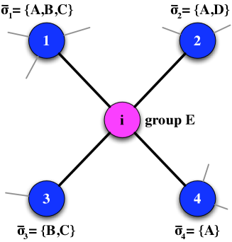
Given the sets associated with the neighbors of a strong node , not all adjacent nodes need to contribute to its full stabilization. Likewise, node can be stabilized by different combinations of its neighbors’ sets . This is best illustrated by an example shown in Fig. 1. Suppose that the groups are and let us assume that node is crisply classified as . Let have four neighbors with corresponding sets , , and . It is clear that all four nodes together must stabilize , as otherwise would not be a strong node. However, the sets of neighbors or each suffice to stabilize node . The node is redundant, since it does not contribute a new class against which or are not already stabilizing. In other words, if the set is considered, node can be removed without altering the stabilization of . The same is not true for the nodes and . The notion of stabilization sets and stabilizer nodes can be defined as follows: A subset of nodes adjacent to is a stabilization set of , if the removal of any one of the nodes from the set causes not to be stabilized by that set anymore. A node is a stabilizer if it is member of at least one stabilization set. The definition of stabilizer involves thus a stabilization relation with at least one of the node neighbors. In the above example, and are the only stabilizers of . Non-stabilizer nodes can be removed without affecting stabilization, while whenever a stabilizer is removed the number of ways in which a given node is stabilized decreases. In the example of Fig. 1, the removal of node would cause complete loss of stabilization of , while removal of or would leave with only a single stabilization. It can be shown that the removal of a stabilizer will never turn a previously non-stabilizer node into a stabilizer, but it might turn some stabilizers into non-stabilizers. Note that in a sense stabilizer is more important than or , since it is part of every stabilization of and its removal will thus render a weak node. In fact, one could attach a strength to each stabilizer by keeping track of the number of stabilizations in which it is involved, but, for sake of simplicity, we will not pursue this here.
Given an NL-EM classification with strong nodes, we can immediately identify the stabilizers that are responsible for the crisp classifications. Details on how to implement the identification of stabilizers are provided in Appendix A.2. The relation stabilizes induces a directed subgraph on the original network and we will refer to this as the stabilizer subgraph. The relation between two stabilizer nodes is not necessarily of mutual stabilization: a necessary condition for adjacent strong nodes and to mutually stabilize each other is that both and are empty. The connections among strong stabilizers capture the relations between groups in the graph. In that sense one can regard the stabilizers as exemplary members of the groups. In the undirected graphs of Figs. 2 - 5 the stabilizer subgraph has been superposed. The extension of these concepts to NL-EM classifications in directed graphs is similar, details are given in Appendix B.
The case of NL-EM classifications into two groups is particularly simple. Denoting the groups as and , a crisply-classified (strong) node belongs to either or and a strong node of a given group has to be stabilized against the complementary group. All nodes with non-empty are therefore stabilizers, and if more than one is present all are equivalent, each stabilizing a given node independently from the other stabilizers. Moreover, the strong stabilizers are nodes that are stabilized themselves by some of their neighbors which necessarily are also stabilizers. The conditions of Eq. (9) permit only two possible configurations of the stabilizer subgraphs. Either strong stabilizers of group connect to strong stabilizers of their own group, or stabilizers of group connect to those of the complementary group . In the former case we get a disjoint community like partition (cf. Fig. 4) of the stabilizer graph, whereas in the latter case we obtain a bipartite partition (cf. Fig. 5).
Furthermore, the NL-EM classification into two groups reveals a simple but meaningful hierarchical structure in the way the different type of nodes in the classification relate. Strong (non-stabilizer) nodes are nodes for which , so these nodes connect to nodes of both groups (weak or strong), however in order for them to be strongly classified as in one group, let us say, () they can only connect to those stabilizer nodes with the compatible stabilizer classes (). In turn, the neighborhood of strong stabilizer nodes with or can consist only of nodes strongly classified as or , respectively. The weak stabilizer nodes are by definition nodes for which , but for which or . Thus weak stabilizer nodes cannot connect to strong stabilizer nodes, but they can stabilize strong (non-stabilizer) nodes. Finally, the weak nodes that are neither strong nor stabilizing can connect to strong non-stabilizing nodes and other weak nodes. In this way the connection rules for the strong stabilizers, weak stabilizers, strong nodes, and weak nodes set up a hierarchy of nodes at the core of which are the strong stabilizers.
4 Stabilizers in a benchmark
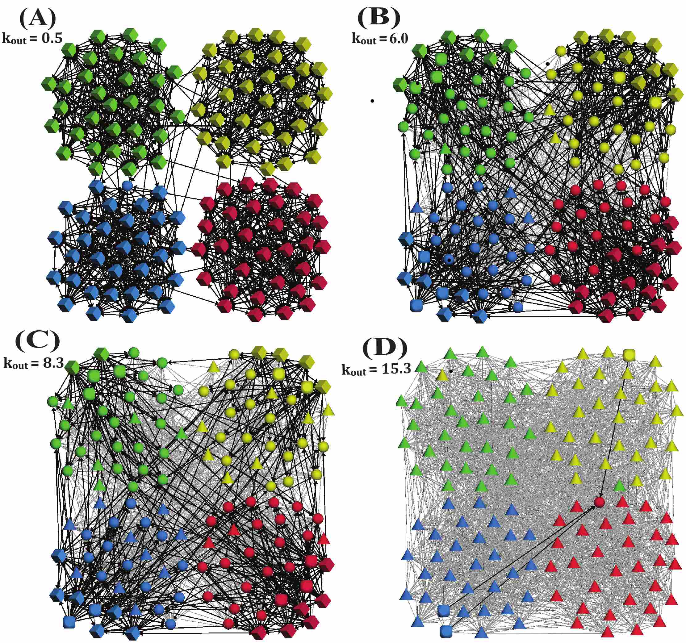
As we observed in the previous section, a node can be stabilized by its neighbors in multiple ways. This redundancy renders classifications robust against disorder introduced by the addition or removal of edges up to a certain point. To illustrate this we consider a benchmark with four communities [11]. The initial network is generated with four disjoint groups of nodes each, with the nodes having on average in-group links. These groups correspond to the four clusters of Fig. 2(A)-(D). Random links connecting different groups are added to the basic configuration and the number of stabilizers are tracked as a function of the average number of out-group links . Fig. 2 shows the stabilizers obtained from an NL-EM classification into groups at disorder level and .
When we find a crisp classification where all nodes are strong stabilizers, meaning that all nodes stabilize and are being stabilized. Furthermore, all of them provide complete stabilization information, , with a single stabilizer sufficing to crisply classify a neighbor. Since , there is on average 16-fold redundancy in the stabilization of each node. As random connections are added to the network, the four clusters become connected with each other. Some of the stabilizers start to stabilize against fewer classes, giving rise to a decrease in the average . In the right panel of Fig. 3, we have plotted how the average stabilization information decays when increases. In order for nodes with to be stabilizers they have to act in combined action with other nodes, as in the example of Fig. 1. Thus an increase of the level of disorder causes both a reduction in the redundancy of stabilizations of strong nodes and a shift towards stabilizations by combined action of more than one stabilizer. The increase in disorder eventually leads to a loss of strong nodes, implying that the classification deteriorates. In order to assess the quality of classifications, we use the entropy , as defined in [2]
| (10) |
The entropy measures the crispness of a classification. When , all the nodes are strong, while corresponds to case where the classification of the nodes is maximally uncertain. The right panel of Fig. 3 displays as a function of , showing that the crispness of the classification is lost for large .
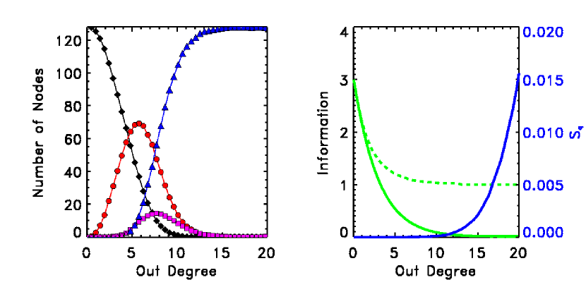
The increase in entropy is closely related to what happens to the different nodes in the classification as edges are added, particularly to the stabilizers. The variation of the number of the different type of nodes with is shown in the left panel of Fig. 3. As the addition of new edges progresses, some nodes cease to be strong stabilizers. When a node is not a strong stabilizer anymore, it can still remain strong as long as there are other nodes stabilizing it in its neighborhood. As can be seen in the left panel of Fig. 3, this is what is happening up to : The number of strong stabilizers decreases while the number of strong nodes rises accordingly. Therefore, initially the effect of adding edges is to convert strong stabilizers into strong nodes. Most of the nodes remain strong (stabilizer or not), and the classification is essentially crisp with an entropy . With the further addition of edges, the number of strong nodes starts to decrease as a result of the loss of stabilization, giving rise to the appearance of weak stabilizing and non-stabilizing nodes at . Continuing to , the entropy of the classification remains very low because there still is a sizable number of strong nodes supported by a few weak and strong stabilizers (see panels B and C in Fig. 2). As further edges are added, the number of weak stabilizers starts to decrease as well, and eventually most of the nodes are weak and non-stabilizing, accounting for the quick rise in the classification entropy starting around .
5 Real-world networks
We focus now on some empirical examples to show the special role that the stabilizers play in a classification and the type of information that they convey while also highlighting the versatility of our analysis. As explained, classifications into two groups are particularly simple and in this case the stabilizers can be easily identified once a solution of the NL-EM clustering is given. This simplicity makes them good candidates to illustrate the properties of the stabilizers. We present first two examples of this type that show the role of the stabilizers and the relations between them. We then turn to a directed network with a classification into groups in order to illustrate a more general situation.
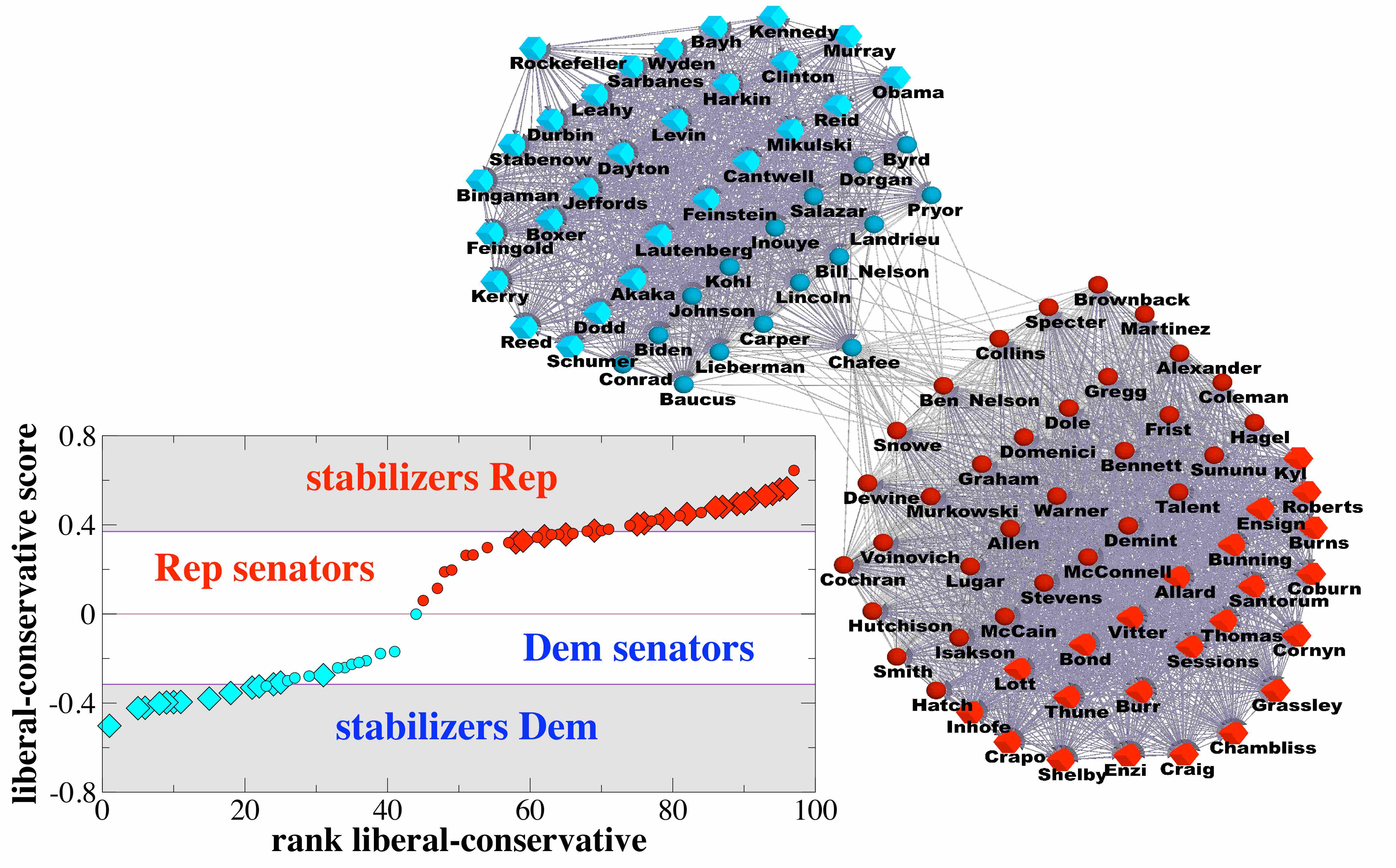
The first example is a network built from the voting records of the th US Senate [31]. The nodes represent senators that served the full two year term () during which issues were voted. Since our aim is to construct a network based on political affinity, we draw an edge between two senators if they voted in the same way at least once. The edges are weighted by the reciprocal of the number of co-voting senators minus one, a common practice for collaboration networks [32]. In this way, an agreement in minority on an issue has a higher value than that in an unanimous vote, differentiating more clearly close political standings. Due to circumstantial quasi-unanimous votes, the network is initially close to fully connected. A threshold such that edges with lower weights are removed can be introduced, and the resulting networks can be analyzed as the threshold increases. We have applied two-group NL-EM to these networks. Once the threshold is high enough, the clusters found follow well the divide between Democrats and Republicans. The instance in which about half of the senators, either Republicans or Democrats, are stabilizers is displayed in Figure 4. Congress roll calls and their derived networks have been extensively studied in the literature [33, 34, 35, 36]. One of the most interesting results is that single votes of a representative can be understood with a low dimensional spatial model (DW-NOMINATE [33, 34]) in which a set of coordinates can be assigned to each congressman characterizing his/her political stand on the different issues. Since the 90’s the number of dimensions required has been reduced in good approximation to only one that strongly correlates with the congressman’s view on socio-economic questions (liberal vs. conservative) [33, 34]. In Fig 4, we show the relation between being a stabilizer and the location in the liberal-to-conservative dimension. The stabilizers tend to be the most radical members of the Senate who are probably defining the overall position of their groups. This exercise can be repeated on networks obtained with different thresholds. It can be seen that as the threshold increases more and more nodes turn into stabilizers. Keeping track of the senators that become stabilizers at different thresholds allows for a refined exploration of the political spectrum. Note in particular that the above results have been obtained by simply looking at the co-voting relation and without considering the vote records in detail, i.e., the actual issue put to vote.
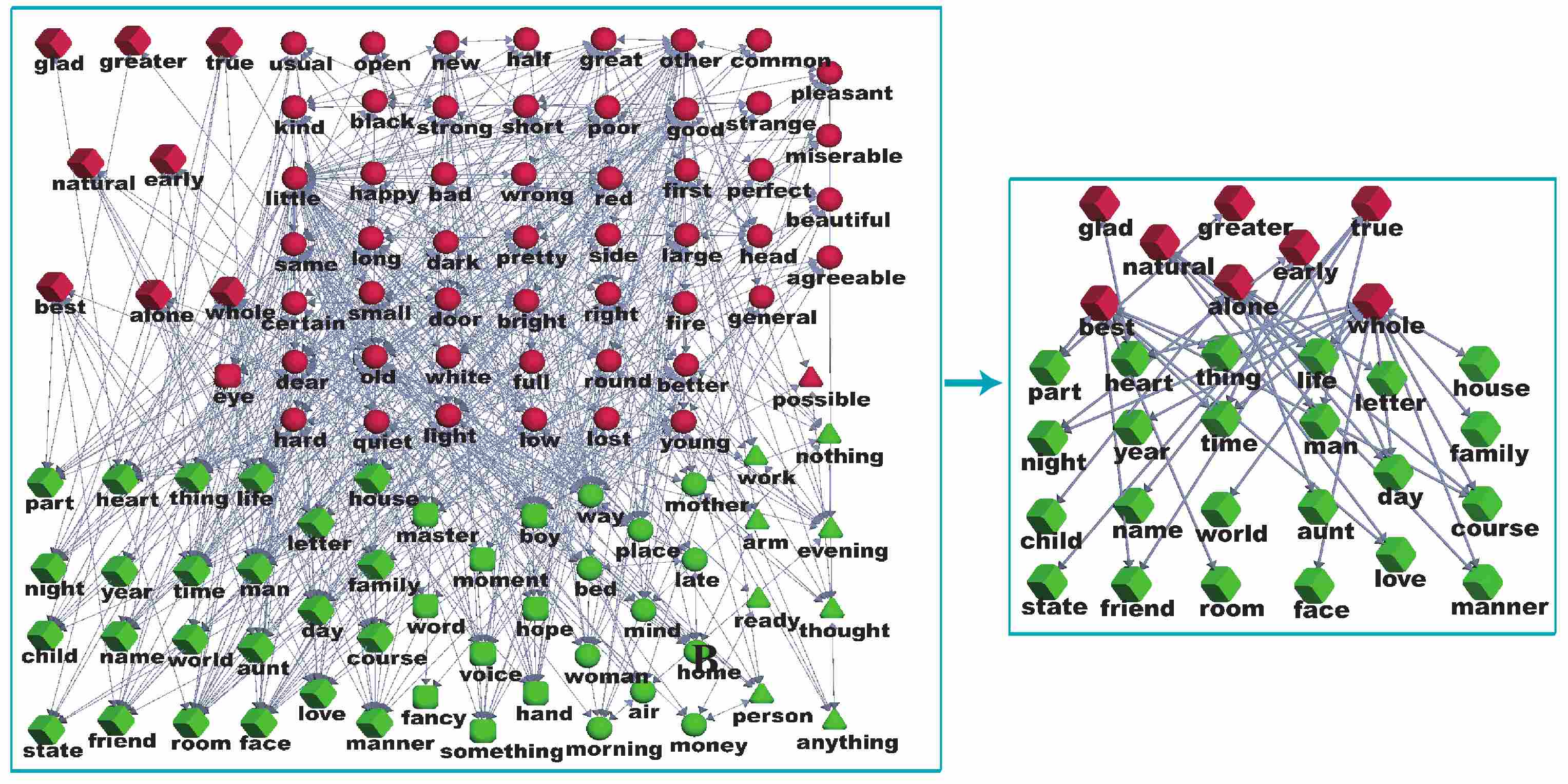
In our second example we show how by extracting the sub-graph of stabilizers we can obtain from its structure useful information about what features distinguish a stabilizer node and how the groups relate in a classification. We consider a semantic network in which the nodes are adjectives and nouns occurring most frequently in Charles Dickens’ novel David Copperfield [37]. A relation between any two of these words is established if they occur in juxtaposition. In Fig. 5, we have represented the network, the best NL-EM partition in two groups and identified the types of nodes. There turn out to be two sub-groups containing nouns or adjectives only that are strong stabilizers. These two sub-groups bear the responsibility for the classification of remaining words by association. Note that the only input to the NL-EM method is the network. We are not introducing any bias for the partition in adjectives and nouns. Most of the remaining words are well classified. The stabilizers, central to establishing the classification, are the words always occurring in strict combinations like true friends, never mixing with members of the same group and they form a bi-partite sub-graph of stabilizers as shown in the right panel of Fig. 5. Conversely, nonstabilizing nodes are words appearing in mixed roles, such as the word little in the adjective-adjective-noun triplet poor little mother.
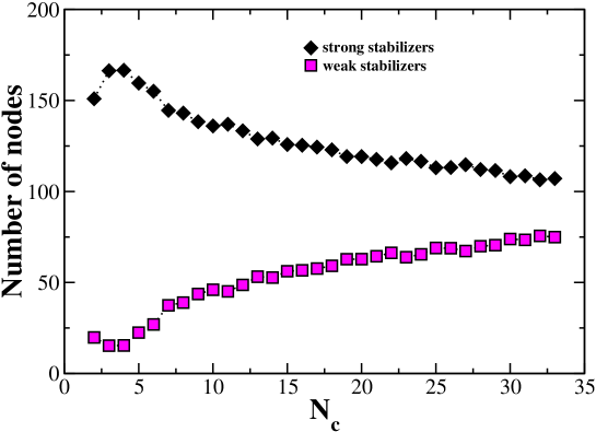
Our final example, showing a more general case with groups, is the Little Rock food-web. The vertices of this network are species living in the aquatic environment of Little Rock Lake in Wisconsin [38]. Each directed link represents a predation relation pointing from predator to prey. The number of trophic levels is around four [39] and turns out to be the number of groups for which the NL-EM algorithm produces a partition with highest abundance of strong stabilizers, as shown in Fig. 6 where we have plotted the number of stabilizers of an NL-EM solution against the number of groups . A property of the four group classification depicted in Fig. 7 is that it keeps basal species (green) in one group, top predators (cyan) in another, and assigns the rest to two different groups based on the prey they feed on at the basal level. The species that are not strong stabilizers, for instance nodes , or , could be related to a missing data problem. In the case of (Hydroporus) or (Lepidoptera Pyralidae), the species appear only as prey having no connection to lower levels. However, its consumers are not typically feeding on basal species, they are ”cyan”, and this results in an NL-EM classification that assigns them into the ”red” group.
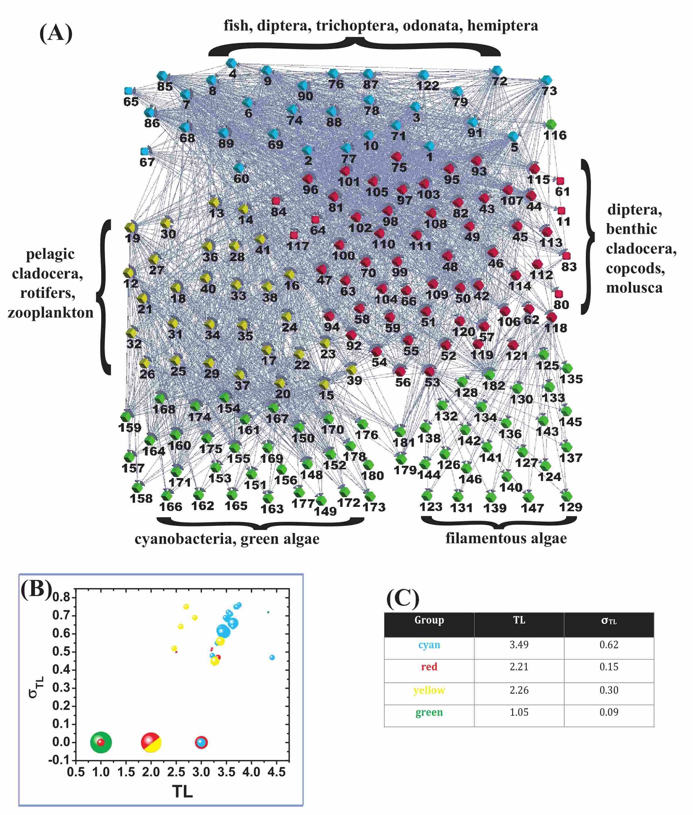
As seen in Fig. 7(A), most of the species of the network are strong stabilizers. Their abundance is a direct result of the highly structured organization of the foodweb: similar species have similar prey which, as our analysis shows, is also linked to their trophic levels (see Fig. 7 B and C). Or more correctly, the consistent choice of species a predator does not prey on is what renders them stabilizers. The possibility of classifying species in low dimensional spaces depending on their trophic level and on the intervality of their prey distribution has been extensively discussed in the literature [8, 40, 41, 42]. Our stability analysis reveals an underling structure in the connectivity pattern of the foodweb, which is responsible for the success of these low dimensional models.
6 Discussion and Conclusions
The maximum likelihood function upon which the NL-EM inference method is based is rather generic and depends on the assumption that nodes with similar connections should be grouped together. Using this likelihood function we were able to show that a subset of nodes, the stabilizers, associated with a given grouping play a central role as they form the backbone of the classification which could not be attained without them. The mathematical basis behind the concept of stabilizers is rather intuitive and follows from the product form of the group assignment probabilities, , in Eq. (7), which is in turn a direct consequence of the assumption that the edges are statistically independent (Eq. (2)). Such an assumption is common to a number of probabilistic clustering methods. We can rewrite Eq. (7) as
| (11) |
where
| (12) |
so that the prefactors are equally absorbed into . Note that is in the interval . Written in the above form it is clear that very small values of must arise from very small values of dominating the product. Likewise, we see from that changes in these factors will have the greatest effect on the value of . The stabilizers we have introduced here constitute the extreme case, namely the nodes for which . As we have shown, this requirement together with the fact that depends in turn on has allowed us to extract the stabilization rules for crisply classified nodes, . However, this concept could be relaxed to define stabilizers more generally by requiring only that with appropriately chosen.
It is possible to apply the notion of stabilizers to other probability models for node classification such as those considered by Airoldi et al.[24] or Nowicki and Snijders [22]. An inspection of Eqs. (2) and (3) as well as the equation for of [24] reveals a similar structure for the inter-relation between the edge-based class assignment probabilities and the class connection probability , which are analogues of the probabilities and . The variational Expectation Maximization approach of [24] can also be applied to a model that was considered by Nowicki and Snijders [22], which is more akin in spirit to the model presented here [43]. For both models, however the resulting rules of stabilization are rather involved due to the inclusion in the likelihood of the absence of edges, as well as due to the non-factorizable form of as compared with Eq. (1). The attractiveness of the probability model, Eqs. (1) and (2), is that it delivers meaningful classifications despite of its simplicity, while at the same time the corresponding stabilization rules have a rather immediate interpretation, as we have shown in Sections 3 and 4.
In summary, we have presented a general method for inferring information about which elements are most relevant in establishing group structures in a complex network. The maximum likelihood function upon which our inference is based is rather generic. This approach does not assume any additional a priori knowledge about the network, rendering it attractive in circumstances in which the available information about the nodes is limited. In particular, we have introduced the concept of stabilizers associated with a given NL-EM classification and shown that they play a central role in the network partition. If the stabilizers were removed from the network, the partition would lose its meaning. If on the other hand, the subgraph formed only by stabilizers is considered, the classification remain intact and useful information regarding the interaction between the different groups in the graph can be obtained. The stabilizers represent therefore the gist of a network partition. Their identification is highly useful in understanding the way in which the structure of complex systems form and their elements aggregate in clusters. This technique has a wide applicability as we have shown with three empirical examples of networks of very different origins: social sciences, semantics and ecology. In addition it raises several important questions, such as the role of these special nodes in the evolution of any dynamic process running on the graph such as the spreading of opinions, rumors or diseases, or even in the evolution of the graph itself if the network is dynamic.
Appendix A Numerical implementation details
A.1 NL-EM algorithm
Given a network, the search for classifications of the NL-EM algorithm was carried out using an algorithm that alternates between simulated annealing and a direct greedy iteration of Eqs. (5) and (7). The program was run with a set of different initial conditions for and for each value of the number of groups . Once the algorithm converged to a stationary value of the likelihood function, the instance with the best was selected.
A.2 Extraction of stabilizers
We outline here the algorithm we have used to extract stabilizers from an NL-EM classification with strong nodes. The problem of determining the set of stabilizers associated with a strong node is related to the set covering problem in Computer Science, which is NP-complete. If a strong node has adjacent nodes with non-empty , there are in principle combinations that have to be checked for finding the fundamental sets leading to stabilizations. In practice, many of the combinations can be eliminated by observing that if, say, have been selected as candidates for a stabilization, any that is a subset of the union of the ’s is redundant and thus cannot be part of that stabilization. This is the main strategy of our algorithm. Also note that, if there are number of classes the number of possible distinct stabilizer sets is . For small , can be larger than so that there are duplicates which can be removed beforehand.
We have used a recursive algorithm for detecting the stabilizers. We partially order the sets by their size. Two binary arrays of size , and indicate the candidates already selected and those available for contribution to a stabilization, respectively. The classes against which the nodes stabilize are coded in an binary array , where the non-zero elements of indicate the classes against which node is stabilizing. A recursively called subroutine , givenin Fig. A.1 in pseudo-code, performs the task of determining all stabilizations of a strong node, given the sets . In the algorithms we have assumed that there is already defined a procedure , which takes a list and returns the indices where the list element equals to along with the number of elements found . Also in our notation when two lists are operated on term by term we denote this as , avoiding having to write out explicitly a loop over the operation on individual elements.

Initially is called with the binary arrays and initialized to zero and one, respectively. The algorithm getNextAvailable (see Fig. A.2) updates , the set of available stabilizers that can contribute to a stabilization after has been added.

Appendix B Extension of NL-EM to directed graphs and stabilization
A generalization of NL-EM to directed graphs that preserves structural equivalence [5, 6, 8] was recently provided in our earlier work [2]. We assume that given a node , a link to a node can be either out-going, in-going or bi-directional. We thus introduce the probabilities:
-
•
that a directed link leaving a vertex of group connects to node ,
-
•
that a directed link pointing to a node in group exists from , and
-
•
that a bidirectional link exiting from group connects to ,
and construct the probability of realizing a directed graph as
| (13) |
, , and are the set of adjacent nodes of from which receives an in-coming, out-going, and bi-directional link, respectively.
The likelihood can now be written as
| (14) |
which has to be maximized under the following constraint on the probabilities ,
| (15) |
implying that there is no isolated node. The probability , that a randomly selected node belongs to group , is again given by . The final result is [2]
| (16) |
| (17) | |||
where , and are the in-degree, out-degree and bi-directional degree of node , respectively.
These expressions have to be again supplemented with the self-consistent equation for which now reads
| (18) |
Note that when we have only bi-directional links so that for all , and it follows from Eq. (17) that . Thus we recover the undirected EM equations Eqs. (5) and (7) under the identification .
B.1 Stabilization rules for directed graphs
The case of directed graphs is similar to the undirected case with a few minor modifications. Given a NL-EM classification of a directed graph , we associate with each node the following four sets:
-
•
, the set of groups that does not have an out-going connection to,
-
•
, the set of groups that does not have an in-going connection to,
-
•
, the set of groups that does not have an bi-directional connection to,
-
•
, the set of groups that does not belong to,
along with their complements, , , , and .
The NL-EM equations, Eqs. 17 and 18, relate the sets and to each other as follows:
| (19) | |||||
| (20) | |||||
| (21) | |||||
| (22) |
Defining the set of all stabilizer classes associated with a node, irrespective of the directionality as
| (23) |
the stabilization condition for a node becomes identical to the one for the undirected case,
| (24) |
References
References
- [1] Newman MEJ and Leicht EA, Mixture models and exploratory analysis in networks, 2007 Proc. Natl. Acad. Sci. USA 104 9564
- [2] Ramasco JJ and Mungan M, Inversion method for content-based networks, 2008 Phys. Rev. E 77 036122
- [3] Rives A and Galitski T, Modular organization of cellular networks, 2003 Proc. Natl. Acad. Sci. USA 100 1128
- [4] Girvan M and Newman MEJ, Community structure in social and biological networks, 2002 Proc. Natl. Acad. Sci. USA 99 7821
- [5] Doreian P, Batagelj V and Ferligoj A, Generalized Blockmodeling, 2005 (Cambridge: Cambridge University Press).
- [6] Lorrain F and White HC, Structural equivalence of individuals in social networks, 1971 Journal of Mathematical Sociology 1 49
- [7] Babu MM, Luscombe NM, Aravind L, Gerstein M and Teichmann SA, Structure and evolution of transcriptional regulatory networks, 2004 Curr. Op. Struct. Biol. 14 283
- [8] R.J. Williams RJ and N. Martinez N, Simple rules yield complex food webs, 2000 Nature 404 180
- [9] Radicchi F, Castellano C, Cecconi F, Loreto V and Parisi D, Defining and identifying communities in networks, 2004 Proc. Natl. Acad. Sci. USA 101 2658
- [10] Fortunato S and Barthélemy M, Resolution limit in community detection, 2007 Proc. Natl. Acad. Sci. USA 104 36
- [11] Newman MEJ and Girvan M, Finding and evaluating community structure in networks, 2004 Phys. Rev. E 69 026113
- [12] Newman MEJ, Modularity and community structure in networks, 2004 Phys. Rev. E 69 066133
- [13] Newman MEJ, Modularity and community structure in networks, 2006 Proc. Natl. Acad. Sci. USA 103 8577
- [14] Arenas A, Díaz-Guilera A and Pérez-Vicente CJ, Synchronization reveals topological scales in complex networks, 2006 Phys. Rev. Lett. 96 114102
- [15] Fortunato S, Community detection in graphs, 2010 Phys. Rep. 486 75
- [16] Clauset A, Moore C and Newman MEJ, Hierarchical structure and the prediction of missing links in networks, 2008 Nature 453 98
- [17] Flake GW, Lawrence S, Giles CL and Coetzee FM, Self-organization and identification of Web communities, 2002 Computer 35 66
- [18] Guimerà R, Mossa S, Turtschi A and Amaral LAN, The worldwide air transportation network: Anomalous centrality, community structure, and cities’ global roles, 2005 Proc. Natl. Acad. Sci. USA 102 7794
- [19] Capocci A, Rao F and Caldarelli G, Taxonomy and clustering in collaborative systems: The case of the on-line encyclopedia Wikipedia, 2008 Europhys. Lett. 81 28006
- [20] Holland PW and Leinhardt S, Local structure in social networks, 1976 Sociological Methodology 7 1
- [21] Wang YJ and Wong GY, Stochastic blockmodels for directed graphs, 1987 J. Am. Stat. Assoc. 82 8
- [22] Nowicki K and Snijders TAB, Estimation and prediction for stochastic blockstructures, 2001 J. Am. Stat. Assoc. 96 1077
- [23] Hastings MB, Community detection as an inference problem, 2006 Phys. Rev. E 74 035102(R)
- [24] Airoldi EM, Blei DM, Fienberg SE and Xing EP, Mixed membership stochastic blockmodels, 2008 Journal of Machine Learning Research 9 1981
- [25] Vazquez A, Population stratification using a statistical model of hypergraphs, 2008 Phys. Rev. E 77 066106
- [26] Vazquez A, Bayesian approach to clustering real value, hypergraph and bipartite graph data: solution via variational methods, 2008 ArXiv:0805.2689
- [27] Zanghi H, Ambroise C and Miele V, Fast online graph clustering via Erdös-Rényi mixture, 2008 Pattern Recognition 41 3592
- [28] Hofman JM and Wiggins CH, Bayesian approach to network modularity, 2008 Phys. Rev. Lett. 100 258701
- [29] Mackay DJC, Information theory, inference and learning algorithms, 2003 (Cambridge: Cambridge University Press).
-
[30]
The question of whether a given graph admits a NL-EM solution
that is a (strong) partition of all of its nodes into groups, can thus be seen as
a coloring problem: We seek a partition of the nodes, i.e. a coloring , corresponding to , such that
is satisfied for all . - [31] Data available at h͡ttp://www.voteview.com
- [32] Newman MEJ, Scientific collaboration networks. II. Shortest paths, weighted networks, and centrality, 2001 Phys. Rev. E 64 016132
- [33] Poole KT and Rosenthal H, Ideology and Congress, 2007 (New Jersey: Transaction Publishers)
- [34] Poole KT, Spatial Models of Parliamentary Voting, 2005 (Cambridge: Cambridge University Press)
- [35] Porter MA, Mucha PJ, Newman MEJ and Warmbrand CM, A network analysis of committees in the U.S. House of Representatives 2005 Proc. Natl. Acad. Sci. USA 102 7057
- [36] Porter MA, Mucha PJ, Newman MEJ and Friend AJ, Community structure in the United States House of Representatives 2007 Physica A 386 414
- [37] Newman MEJ, Finding community structure in networks using the eigenvectors of matrices, 2006 Phys. Rev. E 74 036104.
- [38] Martinez N, Artifacts or Attributes? Effects of Resolution on the Little Rock Lake food web, 1991 Ecological Monographs 61 367
- [39] Williams RJ and Martinez N, Limits to trophic levels and omnivory in complex food webs: theory and data, 2004 The American Naturalist 163 458
- [40] Cattin MF, Bersier LF, Banas̆ek-Richter C, Baltensperger R and Gabriel JP, Phylogenetic constraints and adaptation explain food-web structure, 2004 Nature 427 835
- [41] Stouffer DB, Camacho J and Amaral LAN, A robust measure of food web intervality, 2006 Proc. Natl. Acad. Sci. USA 103 19015
- [42] Allesina S, Alonso D and Pascual M, A general model for food web structure, 2008 Science 320 658
- [43] Mungan M, unpublished