Graphical Models for Correlated Defaults

Abstract

A simple graphical model for correlated defaults is proposed, with explicit formulas for the loss distribution. Algebraic geometry techniques are employed to show that this model is well posed for default dependence: it represents any given marginal distribution for single firms and pairwise correlation matrix. These techniques also provide a calibration algorithm based on maximum likelihood estimation. Finally, the model is compared with standard normal copula model in terms of tails of the loss distribution and implied correlation smile.

1 Introduction

Credit risk concerns the valuation and hedging of defaultable financial securities. (See e.g. Bielecki and Rutkowski [4], Duffie and Singleton [15], Bielecki et al. [5], Lando [31], and the references therein). Since investors almost always engage in a range of different instruments related to multiple firms, successful modeling of the interaction of default risk for multiple firms is crucial for both risk management and credit derivative pricing. The significance of default correlation is highlighted by the current financial crisis.

There are a number of approaches for modeling correlated default. Collin-Dufresne et al. [9], Duffie and Singleton [14] and Schönbucher and Schubert [41] extend the reduced form models by assuming correlated intensity processes. Intensity-based models, however, tend to induce unrealistic levels of correlation. Hull et al. [25], Hull and White [26], and Zhou [48] take the structural form approach and use correlated asset processes, extending the classical framework of Black and Cox [3]. These models nevertheless imply spreads close to zero for short maturities, similar to their single-firm counterparts.

Other approaches for default dependence include the so-called “contagion models”, where default of one firm affects the default process of the remaining firms. For example, Davis and Lo [12] use binary random variables for the default state of each firm, where these random variables are a function of a common set of independent identically distributed binary random variables. Jarrow and Yu [28] extend the reduced form setup by assuming that the intensity for the default process of each firm explicitly depends on the default of other firms, thus one default causes jumps in intensities of other firms’ default processes. Giesecke and Weber [22] place the firms on the nodes of a multi-dimensional lattice, and model their interaction by employing the voter model from the theory of interacting particle systems. The top-down approach, on the other hand, models the credit porfolio as a whole, focusing on the loss process rather than the processes of individual firms. Some examples of this approach include Giesecke and Goldberg [21], Errais et al. [17], Frey and Backhaus [18], Schönbucher and Ehler [40] and Sidenius et al. [42]. These models present their strength in situations where the modeling the individual firm process is not of primary importance: modeling index reference portfolios or when the firms are very small in comparison to the portfolio.

The binomial expansion method [8], Credit Suisse’s CreditRisk$+$ [1], and J.P. Morgan’s CreditMetrics [23] are well-known approaches in the finance industry. While BET represents the loss distribution as a binomial random variable with the number of trials in between the two extremes, CreditMetrics and CreditRisk$+$ focus on individual defaults. Distribution of the random variable representing the state of the firm is parameterized by a set of factors which are shared among the firms, but with varying weights. In contrast, copula models (see Schönbucher [39] for a general survey, and Li [33], Vasicek [44] for the normal copula) separate the modeling of the interdependence of random variables from the modeling of their marginal distributions. Though popular due to its tractability, normal copula suffers from two well-recognized deficiencies: a) it fails to produce fat tails observed in the credit derivatives market for the distribution of number of losses; b) the implied correlations in a normal copula for the equity and senior tranches of a Collateralized Debt Obligation(CDO) are higher than those for the mezzanine tranches, a phenomenon known as the “correlation smile”.

Our work

In this paper, a simple graphical model for correlated defaults is proposed and analyzed (Section 2). This model has an intuitive graphic structure and the loss distribution for its special one-period version is simply a summation of binomial random variables. This model is well posed in capturing default dependence in the following sense: it can represent any given marginal distribution for single firms and pairwise correlation matrix. Techniques from algebraic geometry are employed to prove this well-posedness and to provide a calibration algorithm for the model. Explicit formulas for the loss distribution and for CDO prices are derived. Finally, unlike the standard normal copula approach, this model can produce fat tails for loss distributions and correct the correlation smile (Section 3).

In addition to the proposal and analysis of a simple model for default correlation, one major contribution of this paper is the introduction of a new algebraic technique to study inequalities implied in correlation structures. As correlation in any multi-variate probability distribution naturally leads to certain linear or non-linear inequalities, we are hopeful that this new tool will provide a powerful alternative to existing approaches such as copulas in the mathematical finance literature for analyzing default correlation.

2 The Graphical Model for Defaults

In this section a class of hierarchical models is formulated to model default risk for multiple names. The most generic form of the model is first presented, followed by a specialization to homogeneous parameterizations for ease of calibration and comparison with existing models. To provide context, the simple terminology of “firms”, “sectors” and “default” is adapted, although our model is applicable in any generic context with interaction between multiple entities. In the finance context it includes any type of asset backed security (ABS) on multiple names. For example, one can represent a Collateralized Mortgage Obligation (CMO) with our proposed graph structure, simply by replacing “sectors”, “firms” , and “default” with “geographical region”, “mortgage holder”, and “refinancing or default” respectively.

2.1 General Form

Take an undirected graph $G=(V,E)$ with $M$ nodes, and denote the set of nodes by $V:=\{1,\ldots,M\}$. The edge set $E$ is a subset of ${M\choose 2}$ possible pairwise connections between any pairs of nodes, i.e. $E\subseteq\{(u,v):1\leq u<v\leq M\}$. Each node of the graph corresponds to a firm and has an associated binary random variable $X_{i},\,(i\in V)$ with $X_{i}=1$ representing the default of firm $i$ and $X_{i}=0$ the survival. The joint probability distribution of the random variable $X:=(X_{1},\ldots,X_{M})$ is given by

$$p_{w}(\eta):=P\left(X=w\right) = \frac{1}{Z}\cdot\exp\left(\sum_{i\in V}\eta_{i}w_{i}\,+\sum_{(u,v)\in E}\eta_{uv}w_{u}w_{v}\right)$$ (1)

Here $w=(w_{1},\ldots,w_{M})$ runs over $\{0,1\}^{M}$, the scalars $\eta_{i}\in\mathbb{R}$ and $\eta_{uv}\in\mathbb{R}$ are parameters, and $Z$ is the normalization constant known as the partition function:

$$Z\quad=\,\,\sum_{w\in\{0,1\}^{M}}\exp\,\bigl{(}\,\sum_{i\in V}\eta_{i}w_{i}\,+\sum_{(u,v)\in E}\eta_{uv}w_{u}w_{v}\bigr{)},$$

It is worth mentioning that Kitsukawa et al. [30] and Molins and Vives [35]) have suggested using the long range Ising model (LRIM) in the credit risk context. However, these models are special cases of our formulation, and make use of physical concepts with no clear financial interpretation. They restrict the structure to a single-period model with a completely connected graph and assume that all edge interactions are homogeneous. We investigate heterogeneous connections and a sector model, analyze the multi-period setting, and provide pricing formulas.

Well-posedness of the model

Probabilistic models of the form (1) are also known as Markov random fields, as Ising model in physics, or as graphical models in computer science [29] and statistics [32]. In the finance context, assessment of default correlation is usually assumed to identify the following two sets of sufficient statistics:

• The marginal default probability $P\left(X_{i}=1\right)$ is known for each firm $i\in V$.

• The pairwise linear correlation

  $$\rho_{uv}\,\,\,=\,\,\,\frac{P\left(X_{u}=X_{v}=1\right)\,-\,P\left(X_{u}{=}1\right)\cdot P\left(X_{v}{=}1\right)}{\sqrt{P\left(X_{u}{=}1\right)\cdot\left(1-P\left(X_{u}{=}1\right)\right)\cdot P\left(X_{v}{=}1\right)\cdot\left(1-P\left(X_{v}{=}1\right)\right)}}$$ (2)

  is assumed to be known for all pairs of firms $u$ and $v$ that share an edge in $E$.

Therefore, we shall demonstrate that this model is well posed for modelling correlated default: for every set of marginal default probabilities and correlations, there exists a unique set of parameters matching that information.

Clearly, data on the marginal default probabilities and the pairwise linear correlations is equivalent to the following set of $M+|E|$ sufficient statistics:

• The single node marginals $\,\,P_{i}:=P\left(X_{i}=1\right)\quad$ for all $i\in V$.

• The double node marginals $\,\,P_{uv}:=P\left(X_{u}=X_{v}=1\right)\,\,$ for all $\,(u,v)\in E$.

Denoting this set of marginals by $\,P_{\bullet}\in{[0,1]}^{M+|E|}$, we shall show:

Theorem 1.

Assume any given set of statistics $P_{\bullet}$ from some probability distribution on $M$ binary random variables. Then, there exists a unique set of parameters $\eta_{i},\eta_{uv}$ such that the single and double node marginals implied by Equation (1) match $P_{i},P_{uv}$.

The proof of Theorem 1 relies on techniques from algebraic geometry. The key ingredients of the proof are illustrated through a simple example to gain some insight. These ingredients are essential for model implementation as well (see Section 2.1).

The first ingredient is an integer matrix $A_{G}$ associated with the graph model.

Example 2.

Let $G$ be the triangle with $\,V=\{1,2,3\}\,$and $\,E=\bigl{\{}\{1,2\},\{1,3\},\{2,3\}\bigr{\}}$. The marginals $P_{i}$, $P_{uv}$ are characterized by the following $16$ linear equalities:

$$P_{i}\geq P_{ij}\geq 0\,\,\,\hbox{for all}\,\,i,j,$$

$$P_{1}+P_{2}\,\leq\,P_{12}+1\,,\,\,P_{1}+P_{3}\,\leq\,P_{13}+1\,,\,\,P_{2}+P_{3}\,\leq\,P_{23}+1\,,$$ (3)

$$\,P_{1}+P_{23}\,\leq\,P_{12}+P_{13}\,,\,\,\,P_{2}+P_{13}\,\leq\,P_{12}+P_{23}\,,\,\,\,P_{3}+P_{12}\,\leq\,P_{13}+P_{23}\,,$$

$${\rm and}\quad P_{1}+P_{2}+P_{3}\,\leq\,P_{12}+P_{13}+P_{23}+1.$$

These inequalities can be derived in the following way. First consider the expansion of marginal default probabilities in terms of elementary probabilities $p_{000},p_{001},\ldots,p_{111}$:

$$P_{i}\,\,=\sum_{w\in\{0,1\}^{3}}a_{iw}p_{w}$$

where $a_{iw}\in\{0,1\}$. Then construct a $\{0,1\}$ valued matrix $A_{G}$ using the $a_{iw}$ values, where each row corresponds to a marginal probability, whereas the columns correspond to the elementary probabilities. For the example, this matrix becomes

$$\bordermatrix{&p_{000}&p_{001}&p_{010}&p_{011}&p_{100}&p_{101}&p_{110}&p_{111}\cr P_{1}&0&0&0&0&1&1&1&1\cr P_{2}&0&0&1&1&0&0&1&1\cr P_{3}&0&1&0&1&0&1&0&1\cr P_{12}&0&0&0&0&0&0&1&1\cr P_{13}&0&0&0&0&0&1&0&1\cr P_{23}&0&0&0&1&0&0&0&1}$$ (4)

Then we have

$$\{P_{\bullet}:P_{\bullet}\textrm{ satisfies inequalities~{}(\ref{ineq2})}\}\,=\,\{P_{\bullet}\,:\,P_{\bullet}=A_{G}\cdot p,\,p\in\mathbb{R}_{+}^{8}\,\,{\rm and}\!\sum_{w\in\{0,1\}^{M}}p_{w}=1\}.$$

In other words, the solution set of the $16$ linear inequalities in (3) is the six-dimensional polytope which can be obtained by taking the convex hull of the columns of $A_{G}$.

Remark 3.

If $G$ is the complete graph on $M=4$ nodes then the corresponding $10$-dimensional polytope is described by $56$ facet-defining inequalities. In general, the number of facets of this polytope grows at least exponentially in $M$. See Wainwright and Jordan [45] for an approach which carefully addresses these issues of complexity.

In general, our graphical model can be represented as a toric model as in Geiger et al. [20] or Pachter and Sturmfels [37, §1.2] by defining the appropriate integer matrix $A_{G}$. This matrix represents the linear map which takes the vector of elementary probabilities to the vector of marginals. To be precise the matrix $A_{G}$ has $2^{M}$ columns and $M+|E|+1$ rows and its entries are in $\{0,1\}$. The columns of $A_{G}$ are indexed by the elementary probabilities

$$p_{w}\,=\,p_{w_{1}w_{2}\cdots w_{M}}\,\,=\,\,P(X_{1}=w_{1},\cdots,X_{M}=w_{M}),\,\,\quad w=(w_{1},\ldots,w_{M})\in\{0,1\}^{M}.$$

All rows but the last are indexed by the marginals $P_{i}$ for $i\in V$ and the correlations $P_{uv}$ for $\{u,v\}\in E$. The entries in these rows are the coefficients in the expansion of the marginals in terms of the $p_{w}$. The last row of $A_{G}$ has all entries equal to one, and it corresponds to computing the trivial marginal $\,\sum_{w\in\{0,1\}^{M}}p_{w}=1$.

To be consistent with the algebraic literature, we replace the model parameters by their exponentials, thus obtaining new parameters that are assumed to be positive:

$$\theta_{i}:={\rm exp}(\eta_{i})\,\,\,\hbox{for}\,\,i\in V\quad\hbox{and}\quad\theta_{uv}:={\rm exp}(\eta_{uv})\,\,\,\hbox{for}\,\,\{u,v\}\in E.$$

The model parameterization (1) now translates into the monomial form of [37, §1.2],

$$p_{w}\,\,\,=\,\,\,\frac{1}{Z}\cdot\prod_{i\in V}\theta_{i}^{w_{i}}\cdot\prod_{(u,v)\in E}\theta_{uv}^{w_{u}w_{v}},$$ (5)

where the elementary probabilities are the monomials corresponding to the columns of $A_{G}$. The last row of $A_{G}$ contributes the factor $\frac{1}{Z}$. In multi-dimensional form, the function mapping parameters to the elementary probabilities is then defined as:

$$f:\mathbb{R}^{M+|E|}\rightarrow\mathbb{R}^{2^{M}},\quad\theta\mapsto\frac{1}{\sum_{j=1}^{2^{M}}\theta^{a_{j}}}\left(\theta^{a_{1}},\cdots,\theta^{a_{2^{M}}}\right)$$ (6)

where $\theta^{a_{j}}:=\prod_{i=1}^{M+|E|}\theta_{i}^{a_{ij}}$. The model is the subvariety of the $(2^{M}-1)$-dimensional probability simplex cut out by the binomial equations

$$\prod_{w}p_{w}^{C_{w}}\,-\,\prod_{w}p_{w}^{D_{w}}\,\,\,=\,\,\,0,$$

where $C,D$ run over pairs of vectors in $\mathbb{N}^{2^{M}}$ such that $\,A_{G}\cdot C=A_{G}\cdot D$.

With the new notation, one can represent Example 2 in the following way. $A_{G}$ is the $7{\times}8$-matrix obtained by augmenting (4) with a row of ones. The model parameterization (5) leads to

$$\bigl{(}\,p_{000}\,,\,p_{001}\,,\,p_{010}\,,\,p_{011}\,,\,p_{100}\,,\,p_{101}\,,\,p_{110}\,,\,p_{111}\bigr{)}\qquad\qquad\quad\,$$

$$= \bigl{(}\,1,\,\theta_{3}\,,\,\theta_{2}\,,\,\theta_{2}\theta_{3}\theta_{23}\,,\,\theta_{1}\,,\,\theta_{1}\theta_{3}\theta_{13}\,,\,\theta_{1}\theta_{2}\theta_{12}\,,\,\theta_{1}\theta_{2}\theta_{3}\theta_{12}\theta_{13}\theta_{23}\,\bigr{)}$$

The model is the hypersurface in the seven-dimensional probability simplex given by

$$p_{000}p_{011}p_{101}p_{110}\,\,=\,\,p_{001}p_{010}p_{100}p_{111}.$$ (7)

Next, with this new notation, we introduce the second ingredient of the proof: Birch’s theorem, which implies that this six-dimensional toric hypersurface (7) is mapped bijectively onto the six-dimensional polytope (3) under the linear map $A_{G}$.

Theorem 4 (Birch’s theorem).

Every non-negative point on the toric variety specified by an integer matrix $A$ is mapped bijectively onto the corresponding polytope ${\rm conv}(A)$ under the linear map $A$.

A proof of Birch’s theorem can be found in Appendix A. For a more complete treatment, see e.g. [37, Theorem 1.10]. Now we are ready to prove Theorem 1.

Proof of Theorem 1.

The linear map $A_{G}$ maps the $(2^{M}-1)$-dimensional probability simplex onto the convex hull ${\rm conv}(A_{G})$ of the column vectors of $A_{G}$. The mapping $A\rightarrow conv(A)$ is usually referred to as the marginal map of a log-linear model in statistics (Christensen [7]), or moment map in toric geometry in mathematics (Fulton [19, §4]). The convex polytope ${\rm conv}(A_{G})$ therefore consists of all vectors of marginals that arise from some probability distribution on $M$ binary random variables. Now applying Birch’s theorem to the matrix $A_{G}$ yields the assertion of the theorem. ∎

As a corollary, we conclude by the Main Theorem for Polytopes [47, Theorem 1.1, page 29] that the possible marginals $P_{\bullet}$ arising from Equation (2) are always characterized by a finite set of linear inequalities as in (3). We also note that the above techniques, especially Birch’s theorem, are instrumental for model calibration.

Calibration

There are several algorithms for finding unique model parameters matching any given set of marginal default probabilities and correlations under the general formulation of Equation (1). The calibration problem is equivalent to maximum likelihood estimation for toric models. Indeed, suppose that one is given a data vector $u\in\mathbb{N}^{2^{M}}$ whose coordinates specify how many times each of the states in $\{0,1\}^{M}$ was observed. This data gives rise to an empirical probability distribution with empirical marginals $\,\frac{1}{\sum_{w=1}^{2^{M}}u_{w}}A_{G}\cdot u\,=\,(P_{\bullet})$, where $A_{G}$ is defined as in Section 2.1. The likelihood function of the data $u$ is the following function of model parameters:

$$\mathbb{R}^{M+|E|}\,\rightarrow\mathbb{R}_{>0}\,,\,\,\,\eta\,\,\mapsto\prod_{w\in\{0,1\}^{M}}\!\!p_{w}(\eta)^{u_{w}}.$$ (8)

Here $p_{w}(.)$ is defined as in Equation (1). Thus, a direct consequence of Theorem 1 is

Corollary 5.

The likelihood function (8) has a unique maximizer $\hat{\eta}$. This is the unique parameter vector whose probability distribution implied by Equation (1) has the empirical marginals $(P_{\bullet})$.

The key idea in the proof (given in Appendix B) implies that computing the maximum likelihood parameters amounts to solving the following optimization problem:

$$\max_{\eta}\,\,{{-\sum}_{w\in\{0,1\}^{N}}p_{w}\cdot{\rm log}(p_{w})}$$ (9)

s.t. $$p_{w}=\exp\left(\sum_{i\in V}\eta_{i}w_{i}\,+\sum_{(u,v)\in E}\eta_{uv}w_{u}w_{v}\right)\quad\forall\,w\in\{0,1\}^{M}$$ (11)

$$A_{G}\cdot p=P_{\bullet}$$

Note that on the polytope of all probability distributions $p$ with constraint (11), the objective function (9) as a function of $p$ is strictly concave with its maximizer $\hat{p}$ being the distribution represented by $\hat{\eta}$. One can thus apply convex optimization techniques to solve the parameter estimation problem in our graphical model. In fact, this optimization problem is also known as geometric programming. See Boyd et al. [6] for an introduction to this subject.

Parameter estimation in small toric models can be accomplished with the Iterative Proportional Fitting of Darroch and Ratcliff [10]; see Sturmfels [43, §8.4] for an algebraic description and a maple implementation. Such a straightforward implementation of IPF requires iterative updates of vectors with $2^{M}$ coordinates, which is infeasible for larger values of $M$. To remedy this challenge, one needs to turn to the large-scale computational methods used in machine learning. Popular methods aside from the convex optimization techniques mentioned above include those based on quasi-Newton methods such as LM-BFGS [36], conjugate gradient ascent, log-determinant relaxation [45], and local methods related to pseudolikelihood estimation (particularly in the sparse case).

2.2 One Period Model

For both ease of exposition and numerical comparison with the existing models in literature, we now investigate more specialized forms of the formulation.

First, we impose some structure on the graph. Take $M=N+S$, where nodes $1,\dots,N$ represent individual firms and $N+1,\dots,N+S$ represent individual industry sectors, so that the joint probability distribution for $(X_{1},\cdots,X_{N})$ is defined as:

$$P\left(X_{1}=x_{1},\cdots,X_{N}=x_{N}\right):=\sum_{s\in\{0,1\}^{S}} Q(X_{1}=x_{1},\cdots,X_{N}=x_{N},$$ (12)

$$X_{N+1}=s_{1},\cdots,X_{N+S}=s_{N+S}).$$

Here the probability distribution $Q$ on the right hand side is specified by Equation (1).

Next, to capture the dependency among different industry sectors, we specify the parameters $\eta_{i}$ and $\eta_{uv}$ as follows. We assume that each firm belongs to a particular sector $j=1,2,\cdots,S$ such that firm nodes $\{1,\dots,N\}$ are partitioned into $S$ subsets with $N_{j}$ elements, i.e. $N=\sum_{j=1}^{S}N_{j}$. Moreover, a number of homogeneity assumptions are imposed for simplicity:

• Each firm node $i$ has a single edge, which connects to its respective sector node.

• For any particular sector node $j$, all firm nodes that connect to it have the same node weight $\eta_{F_{j}}$ and same edge weight $\eta_{FS_{j}}$.

• Sector nodes are allowed to have different node weights $\eta_{S_{j}}$, and they can connect to each other with different edge weights $\eta_{N+u,N+v}$.

In short, the probability distribution for $(X_{1},\cdots,X_{N})$ in Equation (12) becomes

$$P\left(X_{1}=x_{1},\dots,X_{N}=x_{N}\right) = \frac{1}{Z_{S}}\sum_{s\in\{0,1\}^{S}}\exp\left(\sum_{j=1}^{S}s_{j}\eta_{S_{j}}+s_{j}n_{j}\eta_{FS_{j}}+n_{j}\eta_{F_{j}}\right)$$ (13)

$$\exp\left(\sum_{(u,v):u,v\in\{1,\cdots,S\}}s_{u}s_{v}\eta_{N+u,N+v}\right)$$

where $n_{j}:=\sum_{i:\eta_{i,N+j}\neq 0}x_{i}$ is the number of defaulting firms in sector $j$, and $Z_{S}$ is the normalization constant. Here a sector random variable $X_{N+j}$ having value $0$ is interpreted as that sector being financially healthy and $1$ as it being in distress.

Note that if the graph $G$ breaks up into various connected components, then the random variables associated with the nodes in each component are independent of each other. This property allows conditional independence structures to be easily incorporated into the model: when the state of all other other firms is fixed, two firms not connected by an edge will default independently of each other. Also note that, by allowing different parameters $\eta_{F_{j}}$ and $\eta_{{FS}_{j}}$ for each sector, one can represent a diverse portfolio of firms, with possibly negative pairwise default correlations.

Some simple calculation yields the loss distribution:

Proposition 6.

Given the model specified by Equation (12),

$$P\left(\sum_{i=1}^{N}X_{i}=n\right) = \frac{1}{Z_{S}}\sum_{(n_{1},\dots,n_{S}):\sum_{j}n_{j}=n}\sum_{s\in\{0,1\}^{S}}\exp\left(\sum_{(u,v):u,v\in\{1,\cdots,S\}}s_{u}s_{v}\eta_{N+u,N+v}\right)$$ (14)

$$\prod_{j}{N_{j}\choose n_{j}}\exp\left(s_{j}\eta_{S_{j}}+s_{j}n_{j}\eta_{FS_{j}}+n_{j}\eta_{F_{j}}\right),$$

where

$$Z_{S} = \sum_{s\in\{0,1\}^{S}}\exp\left(\sum_{j=1}^{S}s_{j}\eta_{S_{j}}+\sum_{(u,v):u,v\in\{1,\cdots,S\}}s_{u}s_{v}\eta_{uv}\right)\prod_{j=1}^{S}\left(1+e^{\eta_{F_{j}}+s_{j}\eta_{{FS}_{j}}}\right)^{N_{j}}.$$

Figure 1: A $12$-firm graph with three sector nodes: Square nodes represent the sectors and circle nodes represent firms.

Connection to Binomial Distribution and Fat Tails

Our model is related to binomial distribution with the simple observation that the probability distribution in Equation (14) can be decomposed into a summation of $2\cdot S$ independent binomial random variables. Indeed, note that when $S=1$,

$$P\left(X_{1}=x_{1},\cdots,X_{N}=x_{N}\right) = \frac{1}{Z_{1}}\left(e^{\eta_{F}\sum_{i}x_{i}}+e^{\eta_{S}+\left(\eta_{FS}+\eta_{F}\right)\sum_{i}x_{i}}\right),$$ (15)

$$P\left(\sum_{i=1}^{N}X_{i}=n\right) = \frac{1}{Z_{1}}{N\choose n}\left[e^{n\eta_{F}}+e^{\eta_{S}+n\eta_{F}+n\eta_{FS}}\right]$$ (16)

$$Z_{1} = \left(1+e^{\eta_{F}}\right)^{N}+e^{\eta_{S}}\left(1+e^{\eta_{F}+\eta_{FS}}\right)^{N},$$ (17)

where $\eta_{FS_{1}},\eta_{S_{1}},\eta_{F_{1}}$ are replaced by $\eta_{FS},\eta_{S},\eta_{F}$ respectively for notational simplicity.

Proposition 7.

Given the model (12), when $S=1$,

$$\sum_{i=1}^{N}X_{i}\stackrel{{\scriptstyle d}}{{=}}YB_{1}+(1-Y)B_{2},$$ (18)

where $Y,B_{1},B_{2}$ are independent and distributed as

$$Y \sim \textrm{Bernoulli}\left(\frac{{e^{\eta_{S}}}\left(1+{e^{\eta_{F}}}{e^{\eta_{FS}}}\right)^{N}}{Z_{1}}\right),$$

$$B_{1} \sim \textrm{Binomial}\left(\frac{{e^{\eta_{F}}}{e^{\eta_{FS}}}}{1+{e^{\eta_{F}}}{e^{\eta_{FS}}}},N\right),$$

$$B_{2} \sim \textrm{Binomial}\left(\frac{{e^{\eta_{F}}}}{1+{e^{\eta_{F}}}},N\right).$$

Corollary 8.

Under the assumptions of Proposition 7,

$$X_{i} \stackrel{{\scriptstyle d}}{{=}} YR_{i}+(1-Y)U_{i},\quad{\rm with}$$ (19)

$$R_{i} \sim \textrm{Bernoulli}\left(\frac{{e^{\eta_{F}}}{e^{\eta_{FS}}}}{1+{e^{\eta_{F}}}{e^{\eta_{FS}}}}\right),$$

$$U_{i} \sim \textrm{Bernoulli}\left(\frac{{e^{\eta_{F}}}}{1+{e^{\eta_{F}}}}\right),$$

and $R_{1},\dots,R_{N},U_{1},\dots,U_{N},Y$ are mutually independent. Moreover,

$$\operatorname{Corr}(X_{1},X_{2}) = \operatorname{Corr}(YV_{1}+U_{1},YV_{2}+U_{2})=\operatorname{Corr}(YV_{1},YV_{2})$$ (20)

$$= \frac{\mathbb{E}[Y^{2}]\mathbb{E}[V_{1}]\mathbb{E}[V_{2}]-\mathbb{E}[Y]^{2}\mathbb{E}[V_{1}]\mathbb{E}[V_{2}]}{\sqrt{\operatorname{Var}(YV_{1})}\sqrt{\operatorname{Var}(YV_{2})}}=\frac{\operatorname{Var}(Y)\mathbb{E}[V]^{2}}{\operatorname{Var}(YV)}$$

$$= \frac{\operatorname{Var}(Y\mathbb{E}[V])}{\operatorname{Var}(YV)}$$

where $V\stackrel{{\scriptstyle d}}{{=}}V_{i}:=R_{i}-U_{i}$ and independent of all other random variables.

One implication of Proposition 7 is that one can have control over the tails of the loss distribution. Of the two binomial random variables, varying the parameters affecting the center of the higher mean random variable to increase(decrease) its mean results in thicker(thinner) tails. Moreover, the loss distribution may be bimodal. Bimodality can be explained by a ‘contagion’ effect among firms. Having a high number of defaults may make it more likely for “neighboring” firms to default. This phenomenon enables our model to correct the so-called “correlation smile” (e.g. Amato and Gyntelberg [2], Hager and Schöbel [24]) in pricing CDOs, since a low probability for mezzanine level defaults naturally lead to lower spreads for the respective tranche. These will be illustrated in detail in Section 3.2.

2.3 Multi-period Model

In this section, we shall extend the one-period model to a multi-period one. This extension is essential for pricing defaultable derivatives and for comparison with standard copula models.

The construction is as follows:

• Start with a single-sector graph with $N$ firms. At each payment period $t_{k}$, the graph evolves by the defaulting of some nodes. Furthermore, some of the previously defaulted nodes are removed. Economically, removal of nodes represents that these firms are no longer influencing or providing useful information about the default process of other firms. Therefore, the number of firms remaining in the system is dynamic, and is denoted by $N_{t_{k}}$. Denote the number of firms that have defaulted up to $t_{k}$ by $D_{t_{k}}$. Then, $D_{0}=0$ and $N_{0}=N$.

• Each defaulted node “stays” in the system for a geometrically distributed number of time steps (with “success” or “removal” probability $p_{R}$), independent of everything else. This is equivalent to removing each defaulted node from the system with probability $p_{R}$, independent of everything else, at the beginning of $t_{k}$. Thus, the number of nodes that are currently in default and still in the system at time $t_{k}$, $I_{t_{k}}$, is given by:

  $${I}_{t_{k}}=D_{t_{k}}+N_{t_{k}}-N$$

• Number of additional defaults $D_{t_{k+1}}-D_{t_{k}}$ during the period $(t_{k},t_{k+1})$ is based on a conditioning of the probability distribution specified by Equation (16). More specifically:

  $$P\left(D_{t_{k+1}}-D_{t_{k}}=n\mid{I}_{t_{k}}=m;N_{t_{k}}\right)$$ (21)

  $$:= \sum_{i_{1},\cdots,i_{n}:i_{j}\in\{m+1,\cdots,N_{t_{k}}\}}P\left(X_{i_{1}}=\cdots=X_{i_{n}}=1,X_{i_{n+1}}=\cdots=X_{i_{N_{t_{k}}}}=0\right.$$

  $$\left.\mid X_{1}=\cdots=X_{m}=1\right),\quad n+m\leq N_{t_{k}}$$

This construction, together with some simple calculation, leads to

Proposition 9.

$$P\left(D_{t_{k+1}}-D_{t_{k}}=n\mid{I}_{t_{k}}=m;N_{t_{k}}\right)=\tilde{P}\left(n;N_{t_{k}}-m,\eta_{S}+m\eta_{FS},\eta_{FS},\eta_{F}\right)$$

where

$$\tilde{P}\left(n;N,\eta_{S},\eta_{FS},\eta_{F}\right):=P\left(\sum_{i=1}^{N}X_{i}=n\right)$$

as defined by Equation (16) and

$$Z_{N,\eta_{S},\eta_{FS},\eta_{F}}:=Z_{1}$$

as defined by Equation (17).

2.3.1 Simulation and CDO pricing

Based on the above proposition, it is easy to see that this multi-period model can be simulated as follows. At time $0$, the graph has $N$ non-defaulted firms, At time $t_{1}$, no removal of nodes occurs since none of the firms were in default at time $0$. The number of firms that default during period $(0,t_{1})$, $D_{1}-D_{0}=D_{1}$ is determined by sampling from Equation (16). At time $t_{2}$, each of the $D_{1}$ nodes is removed from the graph with probability $p_{R}$. The additional number of defaults $D_{2}-D_{1}$ is determined by Equation (21), where $N_{2}$ is the total number of firms remaining after the removal, and ${I}_{t_{2}}$ is the number of firms among $D_{1}$ that have not been removed from the graph. Continue in this fashion until $K$ periods are covered.

Moreover, the homogeneity assumptions for the one-period single-sector model imply that our model can be perceived as a two-state discrete time Markov chain, as $(D_{t_{k+1}},N_{t_{k+1}})$ only depends on $(D_{t_{k}},N_{t_{k}})$. Indeed, the transition matrix $P$ of the Markov chain is given by:

$$P_{(D_{t_{k}},N_{t_{k}})\rightarrow(D_{t_{k+1}},N_{t_{k+1}})} = {I_{t_{k}}\choose N_{t+k}-N_{t_{k+1}}}p_{R}^{N_{t_{k}}-N_{t_{k+1}}}{(1-p_{R})}^{D_{t_{k}}-N+N_{t_{k+1}}}$$

$$\tilde{P}(D_{t_{k+1}}-D_{t_{k}};N_{t_{k}}-{I}_{t_{k}},\eta_{S}+{I}_{t_{k}}\eta_{FS},\eta_{FS},\eta_{F})$$

$$N\geq D_{t_{k+1}}\geq D_{t_{k}}\geq 0\textrm{ and }N\geq N_{t_{k}}\geq N_{t_{k+1}}\geq 0$$

with $D_{0}=0,N_{0}=N$. This Markov chain formulation is useful for analytical calculation of loss distribution and CDO prices.

For purposes of model comparison in the later sections, we briefly discuss pricing of CDOs in our model.

Collateralized Debt Obligation(CDO) Pricing

A Collateralized Debt Obligation (CDO) is a portfolio of defaultable instruments (loans, credits, bonds or default swaps), whose credit risk is sold to investors who agree to bear the losses in the portfolio, in return for a periodic payment. A CDO is usually sold in tranches, which are specified by their attachment points $K_{L}$ and detachment points $K_{U}$ as a percentage of total notional of the portfolio. The holder of a tranche is responsible for covering all losses in excess of $K_{L}$ percent of the notional, up to $K_{U}$ percent. In return, the premiums he receives are adjusted according to the remaining notional he is responsible for. In the case of popularly traded tranches on the North American Investment Grade Credit Default Swap Index (CDX.NA.IG), the tranches are named equity, mezzanine, senior, senior, super-senior with attachment and detachment points of $0-3,3-7,7-10,10-15,15-30$ respectively.

Given an underlying portfolio, and fixed attachment and detachment points for all tranches, the pricing problem is the determination of periodic payment percentages (usually called spreads) $s_{l}$ for all tranches, assuming the market is complete and default-free interest rate is independent of the credit risk of securities in the portfolio.

If we denote the total notional of the portfolio by $M$, the periodic payment dates by $t_{1},\dots,t_{K}$, the date of inception of the contract by $t_{0}:=0$, payment period $t_{k+1}-t_{k}$ by $\gamma$, the total percentage of loss in the portfolio by time $t_{k}$ by $C_{t_{k}}$, the attachment (detachment) point for tranche $l$ by $K_{L_{l}}$ ($K_{U_{l}}$), and the discount factor from $t_{0}$ to $t_{k}$ by $\beta(t_{0},t_{k})$, then it is clear that specifying the distribution for $C_{t_{k}}$ for $k=1,\dots,K$ is sufficient for pricing purposes.

To see this, note the percentage of loss $C_{l,t}$ suffered by the holders of tranche $l$ up to time $t$ is given by:

$$C_{l,t} := \min\{C_{t},K_{U_{l}}\}-\min\{C_{t},K_{L_{l}}\}.$$ (23)

Consequently, the value at time $t_{0}$ of payments received by the holder of tranche $l$ is

$$\sum_{k=1}^{K}\beta(t_{0},t_{k})s_{l}\gamma M\mathbb{E}[K_{U_{l}}-K_{L_{l}}-C_{l,t_{k}}].$$ (24)

Similarly, the value at time $t_{0}$ of payments made by the holder of tranche $l$ is given by

$$\sum_{k=1}^{K}\beta(t_{0},t_{k})M\mathbb{E}[C_{l,t_{k}}-C_{l,t_{k-1}}].$$ (25)

In order to prevent arbitrage, the premium $s_{l}$ needs to be chosen such that the value of payments received is equal to the value of payments made. Therefore,

$$s_{l} = \frac{\sum_{k=1}^{K}\beta(t_{0},t_{k})\left(\mathbb{E}[C_{l,t_{k}}]-\mathbb{E}[C_{l,t_{k-1}}]\right)}{\sum_{k=1}^{K}\beta(t_{0},t_{k})\gamma\left(K_{U_{l}}-K_{L_{l}}-\mathbb{E}[C_{l,t_{k}}]\right)}.$$ (26)

Now our focus is to calculate the distribution for $C_{t_{k}}$ in our multi-period model. Denoting the $k$-step transition matrix (in Equation (2.3.1)) for the Markov chain with $P^{k}$ and the number of losses at the $k$-th step by $L^{k}$, then

$$P\left(C_{t_{k}}=\frac{m}{N}\right)=P\left(L^{k}=m\right)=\sum_{n=0}^{N}P^{k}_{(0,N)\rightarrow(m,n)},$$ (27)

and the spreads are given by

Proposition 10.

Given the yield curve $\beta$, attachment ($K_{L_{l}}$) and detachment ($K_{U_{l}}$) points, and the implied Markov transition matrix $P$, the spread of tranche $l$ is

$$s_{l} = \frac{\sum_{k=1}^{K}\beta(t_{0},t_{k})\left(\sum_{m=0}^{N}\left(\min\{\frac{m}{N},K_{U_{l}}\}-\min\{\frac{m}{N},K_{L_{l}}\}\right)\sum_{n=0}^{N}P^{k}_{(0,N)\rightarrow(m,n)}-P^{k-1}_{(0,N)\rightarrow(m,n)}\right)}{\sum_{k=1}^{K}\beta(t_{0},t_{k})\gamma\left(K_{U_{l}}-K_{L_{l}}-\sum_{m=0}^{N}\left(\min\{\frac{m}{N},K_{U_{l}}\}-\min\{\frac{m}{N},K_{L_{l}}\}\right)\sum_{n=0}^{N}P^{k}_{(0,N)\rightarrow(m,n)}\right)}.$$

3 Sensitivity Analysis and Comparison with One-Factor Normal Copula

In this section, some numerical results on the proposed model are reported, and they are compared with both the static(one-period) and dynamic(multi-period) one-factor normal copula model. Throughout the section, $S=1$ is assumed for simplicity.

3.1 Static Characteristics

Correlation for single-period model

First, we analyze the effects of the parameterization triplets $(\eta_{S},\eta_{F},\eta_{FS})$ on the correlation between two firms $corr(X_{i},X_{j})$. Note the following statement

Proposition 11.

Given fixed $\eta_{S},\eta_{FS}$ and $q\in(0,1)$, the $\eta_{F}^{*}$ value that gives $P\left(X_{1}=1\right)=q$ in Equation (15) is given by

$$g(e^{\eta_{F}^{*}})+e^{\eta_{S}}g\left(e^{\eta_{FS}}e^{\eta_{F}^{*}}\right)=0,$$

where

$$g(y)=\left(1-\frac{1-q}{q}y\right)\left(1+y\right)^{N-1}.$$

Take $q=0.01,0.05$ and $N=125$. Figures 2–5 show the correlation values for the four quadrants on $\eta_{S}$ and $\eta_{FS}$. For each point Proposition 11 is utilized for calculating the $\eta_{F}^{*}$ value that achieves the desired $q$ value. Note that $\eta_{FS}$ is the dominant parameter when $\eta_{FS}$ values are close to $0$. As $\eta_{FS}$ moves away from $0$, $\eta_{S}$’s effect increases. Also note that it is possible to obtain high degrees of linear correlation levels even for $q=0.01$. This extends the abilities of multi-firm extensions of intensity-based models in literature (see [39, §10.5] for a discussion).

(a) q=$0.01$

(b) q=$0.05$

Figure 2: Variation of $\rho$ for fixed marginal default probabilities, $\eta_{S}<0,\eta_{FS}>0$

(a) q=$0.01$

(b) q=$0.05$

Figure 3: Variation of $\rho$ for fixed marginal default probabilities, $\eta_{S}<0,\eta_{FS}<0$

(a) q=$0.01$

(b) q=$0.05$

Figure 4: Variation of $\rho$ for fixed marginal default probabilities, $\eta_{S}>0,\eta_{FS}>0$

(a) q=$0.01$

(b) q=$0.05$

Figure 5: Variation of $\rho$ for fixed marginal default probabilities, $\eta_{S}>0,\eta_{FS}<0$

Loss distribution for single-period model

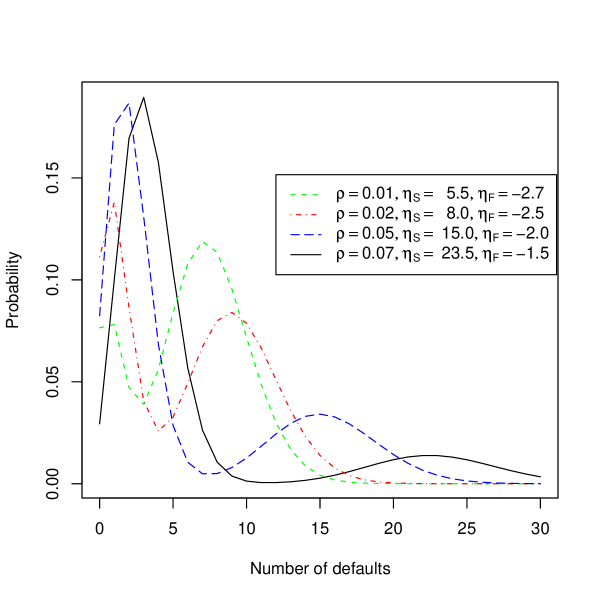
Figure 6 exhibits the shape and fat tails of the loss distribution for different parameters. Here $N=$125, $\eta_{FS}=$ -2.1, $P\left(X_{i}\right)=$0.05, with $\eta_{S}$ calibrated to match the given correlation level $\rho$ and $\eta_{F}$ to match the given marginal default probability. The figure shows the loss distribution for correlation levels 0.01, 0.02, 0.05, 0.07. As expected, the mass shifts towards the tail as correlation increases. All the distributions are bimodal, which facilitates having significantly fat tails.

Figure 6: Distribution of number of defaults under different correlations, $\eta_{FS}=$-2.1, $\eta_{S},\eta_{F}$ varying

Heavy Tails for Multi-period Model

(a) Single step loss distribution

(b) 5 steps

(c) 10 steps

Figure 7: Evolution of number of defaults for varying disappearance probabilities, $\eta_{F}$=-2.8, $\eta_{S}$=5.514, $\eta_{FS}$=-5, $\rho$=0.05, single step default probability 0.005, 50 firms

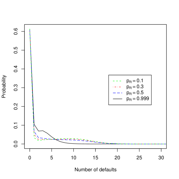
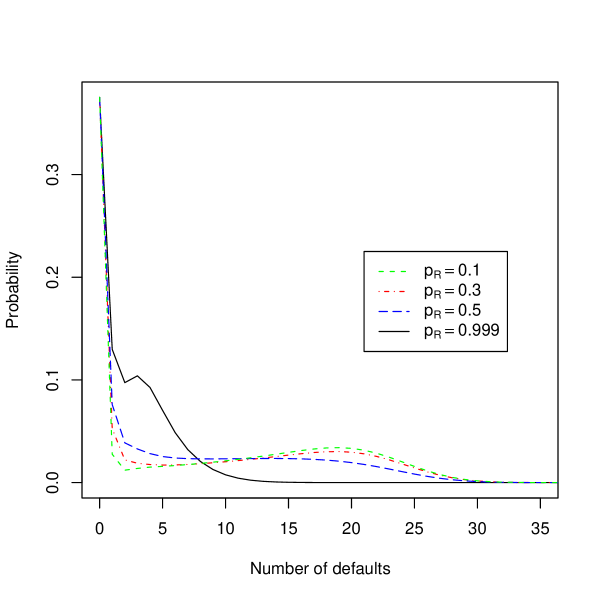
Figure 7 shows the effect of different parameterizations on loss distributions in a multi-period model. Take $N=$50 firms and $(\eta_{S},\eta_{FS},\eta_{F})$= $($5.514, -5, -2.76$)$. The parameters are chosen to correspond to the single-firm default probability of 0.005 and default correlation of 0.05. The loss distribution is then calculated after 5 and 10 steps, with the removal probabilities $p_{R}$ = 0.1, 0.3, 0.5, 0.999. Note that by varying $p_{R}$, tail of the loss distribution can be controlled as shown in Figure 7: Increasing $p_{R}$ results in thinner tails, whereas lower $p_{R}$ values can obtain quite fat tails. As the removal probability increases, the mass is shifted towards fewer defaults. This is intuitive, since higher $p_{R}$ values lead to defaulted firms staying in the system shorter and thus having less detrimental effect on financially healthy firms. Moreover, the tails become very significant as the number of steps increase, despite a relatively low single-step default probability of 0.005. Figure 7(c) shows the importance of choosing a suitable single step default probability. High values for this quantity results in rather strong shifts of mass towards high number of defaults. Therefore, for a fixed maturity, whenever the number of steps is increased, the single step default probability has to be scaled down accordingly.

3.2 Comparison to Normal Copula

In this section, we compare our model with the widely used one-factor normal copula model of [33]. Two important attributes are discussed: the heaviness of the tails in loss distribution, and the correlation smile in pricing standard tranches.

Heavy tails for One-period Model

One well-known deficiency of normal copulas with a constant correlation parameter for all pairs of firms is the thinner “tails” in the loss distribution than observed from market data. In comparison, Proposition 7 suggests that the loss distribution based on our model can achieve fatter tails.

To demonstrate this, first recall that in a copula model, the default indicator $X_{i}$ for firm $i$ is given by $X_{i}=\mathbb{I}\{M_{i}\leq K\}$ where

$$M_{i} = \sqrt{\rho_{A}}Y+\sqrt{1-\rho_{A}}\epsilon_{i},\,i\in\{1,\cdots,N\}$$ (28)

$$Y,\epsilon_{i} \sim \textrm{Normal}(0,1)\,\,i.i.d.$$

$\rho_{A}=corr(M_{i},M_{j})$ is the asset correlation, assumed to be the same for all pairs of firms. Note that $K\in\mathbb{R}$ implicitly specifies the marginal default probability $P\left(X_{i}=1\right)$ which is assumed to be the same across all firms. Note also that the asset correlation $\rho_{A}$ is different from the default correlation $\rho=corr(X_{i},X_{j})$ which is given by:

$$\rho=\frac{{\Phi^{-1}(K)}^{2}\int_{-\infty}^{\infty}\phi(y){\Phi\left(\frac{K-\sqrt{\rho_{A}}y}{\sqrt{1-\rho_{A}}}\right)}^{2}dy}{{\Phi(K)}^{2}{(1-\Phi(K))}^{2}}.$$

This is an important distinction, as asset correlation values for the normal copula result in significantly different values of default indicator correlation.

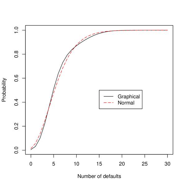
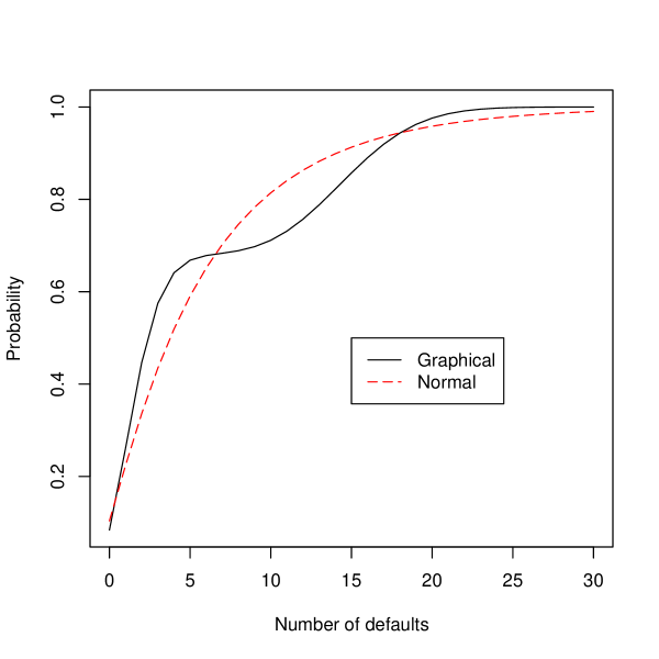
For comparing loss distributions implied by the two approaches, take $N=$125, $P\left(X_{i}=1\right)=$ 0.05, and two levels of $\rho=$ 0.01, 0.05. For the normal copula, these $\rho$ values lead to to $\rho_{A}$=0.042, 0.18 respectively. For our model, take $(\eta_{FS},\eta_{S},\eta_{F})=\\ ($-0.95, 9.2, -2.2$)$ and $($ -2.1, 15, -2$)$ respectively. These parameters are chosen so as to match the specified $P\left(X_{i}=1\right)$ and $\rho$. For both levels of correlation, as demonstrated in Figure 8 our model exhibits fatter tails and has smaller loss probabilities for intermediary values. Furthermore, the values for the loss distribution are of the same scale. All these properties help in correcting the deficiencies of the normal copula when pricing CDO’s, as demonstrated next.

(a) $\rho=0.01$

(b) $\rho=0.05$

Figure 8: Comparison of one-factor normal copula and single sector one-period graphical models

Correlation Smile

For the normal copula, the pricing scheme of [33] and Hull and White [27] is utilized, where the default time $\tau_{i}$ for a firm is defined through a transformation of $M_{i}$ in Equation (28). More specifically, the risk-free interest rate $r$ and the recovery rate $R$ are taken to be constants, $\tau_{i}$ is assumed to be distributed exponentially with rate $\lambda$, and $M_{i}$ is mapped to $\tau_{i}$ using a percentile-to-percentile transformation so that for any given realization $\hat{M}_{i}$:

$$\hat{\tau}_{i} = \frac{-\ln(1-\Phi(\hat{M}_{i}))}{\lambda}.$$ (29)

The spreads $s_{l}$ are then calculated by simulating $M_{i}$ values and replacing the expected values in the pricing formula in Equation (26) by their respective estimators.

Recall that given a standard tranche on CDX.NA.IG, with given observed spread $s_{l}$, and known $r,R,\lambda$, it is possible to “imply” the asset correlation parameter $\rho_{A}$ in Equation (28). However, it is known (e.g. [2], [24]) that implying $\rho_{A}$ in such a manner across all tranches results in a “smile”: The mezzanine tranche has lower implied correlation compared to the neighboring tranches. One plausible interpretation for this kind of smile is that the normal copula model underprices the senior tranches and overprices the equity tranche in comparison to the mezzanine tranche.

We now demonstrate that our model has the potential to correct this smile. To achieve this, first we calculate prices from normal copula. We then find parameters $(\eta_{F},\eta_{FS},\eta_{S},p_{R})$ such that our model matches the mezzanine tranche spread exactly with those from normal copula while giving significantly lower spreads for the equity tranche and higher spreads for the senior tranches.

More specifically, take two different credit rating classes, representing high and low credit ratings respectively, so that

• the one-year default probabilities are set at 0.001 for high-rating class and 0.015 for low-rating class,

• the asset correlation values for the normal copula are 0.2 and 0.3 (these values correspond to default indicator correlations of 0.0059 and 0.0562 ),

• the recovery rate is 0.4, the interest rate 0.05, and $N$=50,

• the maturity of the CDO is 5 years with payment frequency 0.5 corresponding to a ten period model.

Meanwhile, for each rating class, an optimization on $(\eta_{FS},\eta_{S},p_{R})$ maximizing the difference between equity tranche spread for the normal copula and our model, and senior tranche spreads for our model and the normal copula is run. Parameter $\eta_{F}$ is constrained so that both the one-year default probability and the mezzanine spread are matched.

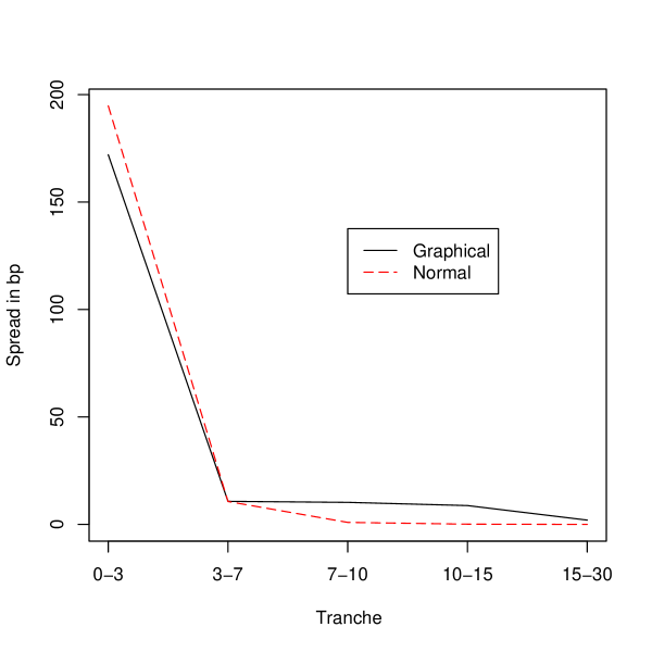
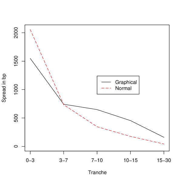
Figure 9 shows the output of one such optimization run. It demonstrates that even with a flat correlation value for the graphical model, one can obtain lower prices for mezzanine tranche and higher for the senior tranches in comparison to the normal copula, thus “correcting” the correlation smile.

(a) High-rating CDO

(b) Low-rating CDO

Figure 9: Tranche spreads for graphical and normal copula models

4 Conclusion

This paper proposes and analyzes a simple graphical model for modelling correlated default. The graphical representation provides an effective shorthand to depict the dependence relationships between the $N$ firms, with the desirable conditional independence property. The probability distribution proposed is a toric model which is beneficial in both parameter estimation and simulation. With some homogeneity assumptions, loss distributions and CDO prices are obtained analytically. The model generates heavy tails in the loss distribution, and its dynamic formulation seems promising for correcting the correlation smile observed in one-factor normal copula.

Appendix A Birch’s Theorem

Our proof follows that in [19], and begins with a lemma.

Lemma 12.

Let $A=(a_{ij})$ be a real $d\times m$ matrix of rank $d$ and $\operatorname{pos}(A)$ the $\mathbb{R}_{\geq 0}$-span of its columns $a_{\cdot 1},\dots,a_{\cdot m}$. Let $t^{1},\dots,t^{m}\in\mathbb{R}_{>0}$ be real positive numbers and define

$$F:\mathbb{R}^{d}\rightarrow\mathbb{R}^{d}$$

$$\eta\mapsto\sum_{j=1}^{m}t^{j}e^{\langle a_{\cdot j},\eta\rangle}a_{\cdot j}$$

That is, $F(\eta)=A(t^{1}e^{\langle a_{\cdot 1},\eta\rangle},\dots,t^{m}e^{\langle a_{\cdot m},\eta\rangle})^{\top}$. Then $F$ determines a real analytic isomorphism of $\mathbb{R}^{d}$ onto the interior of $\operatorname{pos}(A)$.

Proof.

First, the fact that $F$ is an injective local isomorphism with image points arbitrarily close to the extreme rays of $\operatorname{pos}(A)$ is established. Then the result will follow from an inductive proof that $\operatorname{im}(F)$ is convex.

We have $F(\eta)_{i}=\sum_{j}t^{j}e^{a^{\ell}_{j}\eta_{\ell}}a^{i}_{j}$, so

$$\frac{\partial F_{i}}{\partial\eta_{k}}=\sum_{j}t^{j}e^{a^{\ell}_{j}\eta_{\ell}}a^{i}_{j}a^{k}_{j}$$

so that the Jacobian is symmetric. Moreover, the quadratic form is given by

$$x_{i}(t^{j}e^{a^{\ell}_{j}\eta_{\ell}}a^{i}_{j}a^{k}_{j})x_{k}=(x_{i}a^{i}_{j})t^{j}e^{a^{\ell}_{j}\eta_{\ell}}(a^{k}_{j}x_{k})=t^{j}e^{a^{\ell}_{j}\eta_{\ell}}(x_{i}a^{i}_{j})^{2}$$

which is strictly positive for $x\not=0$ since the $a^{\cdot}_{j}$ span $\mathbb{R}^{d}$, so some $a^{i}_{j}\neq 0$. This shows that $F$ is a local isomorphism. To show it is injective, it is sufficient to check that $F$ is injective on a line, and by a change of coordinates this reduces the problem to the case $d=1$. In this case, the $a^{\cdot}_{j}$ are scalars $a_{j}$ and $F$ sends $\eta\in\mathbb{R}$ to $t^{j}a_{j}e^{a^{i}_{j}\eta_{i}}$, with strictly positive derivative as above. $\operatorname{pos}(A)$ is either $[0,\infty)$, $(\infty,0]$, or $(-\infty,\infty)$ depending on the signs of the $a_{j}$, and $F$ is an isomorphism of manifolds. Thus the $d=1$ case shows $F$ is injective and will also serve as the base case for our induction.

By grouping the $a^{\cdot}_{j}$ and changing the $t^{j}$, one may assume no two $a^{\cdot}_{j}$ lie on the same ray. Suppose $a^{\cdot}_{1}$ generates an extreme ray of $\operatorname{pos}(A)$. Then one may choose $v$ such that $\langle v,a^{\cdot}_{1}\rangle=0$ but $\langle v,a^{\cdot}_{1}\rangle<0$ for $j\neq 1$. Then $F(\lambda v+\eta)=t^{1}e^{\langle\eta,a^{\cdot}_{1}\rangle}a^{\cdot}_{1}+\cdots+t^{1}e^{\langle\eta,a^{\cdot}_{1}\rangle+\lambda\langle v,a^{\cdot}_{m}\rangle}a^{\cdot}_{m}$, so

$$\lim_{\lambda\rightarrow\infty}F(\lambda v+\eta)=t^{1}e^{\langle\eta,a^{\cdot}_{1}\rangle}a^{\cdot}_{1}$$

so that one can approach any point on $\mathbb{R}_{\geq 0}a^{\cdot}_{1}$ arbitrarily closely by adjusting $\eta$.

It remains to show that the image of $F$ is convex. Suppose $\operatorname{im}(F)$ is convex for $d-1$, and let $L$ be a line in $\mathbb{R}^{d}$; to show $\operatorname{im}(F)$ is convex for $d$, one must show that $L\cap\operatorname{im}(F)$ is connected or empty. One can write $L=\pi^{-1}q$ for a suitable projection $\pi:\mathbb{R}^{d}\rightarrow\mathbb{R}^{d-1}$ and point $q\in\mathbb{R}^{d-1}$, and

$$\operatorname{im}(F)\cap L=F(\mathbb{R}^{d})\cap\pi^{-1}(q)=F((\pi\circ F)^{-1}(q)).$$

By a linear change of coordinates in $\mathbb{R}^{d}$, one may assume that $\pi$ is projection onto the first $d-1$ coordinates. Let $\rho$ denote the projection to the last coordinate, $\eta\mapsto\eta_{d}$. Let $G=\pi\circ F$ and for $y\in\mathbb{R}$ let $G_{y}$ be the restriction of $G$ to $\rho^{-1}y$.

This defines a map $G_{y}:\mathbb{R}^{d-1}\rightarrow\mathbb{R}^{d-1}$. $G_{y}(\eta_{1},\dots,\eta_{d-1})=\sum_{j}s^{j}e^{\eta_{\hat{d}}\cdot a^{\hat{d}}_{j}}a^{\hat{d}}_{j}$ with $s^{j}=t^{j}e^{ya^{d}_{j}}>0$. Still the columns of its defining matrix $\hat{A}$ ($A$ without its last row) span $\mathbb{R}^{d-1}$, so $G_{y}$ meets the hypotheses of the theorem for $d-1$. Thus each $G_{y}$ is an injective map onto $\operatorname{int}(\pi(\operatorname{pos}(A)))$. Then for each $q$ in $\operatorname{int}(\pi(\operatorname{pos}(A)))$, the projection $G^{-1}(q)=(\pi\circ F)^{-1}(q)$ to $\mathbb{R}$ induced by $\rho$ is a bijection. So the intersection is connected. ∎

Now Lemma 12 can be applied to polytopes.

Proposition 13.

Let $A=(a_{ij})$ be a real $d\times m$ matrix, and $K$ be the convex hull of its columns $a_{\cdot 1},\dots,a_{\cdot m}$. Further require that the $a_{\cdot j}$ not be contained in any hyperplane. Let $t_{1},\dots,t_{m}\in\mathbb{R}_{>0}$ be real positive numbers and define

$$H:\mathbb{R}^{d}\rightarrow\mathbb{R}^{d}$$

$$\eta\mapsto\frac{1}{Z(\eta)}\sum_{j=1}^{m}t^{j}e^{\langle a_{\cdot j},\eta\rangle}a_{\cdot j}$$

where $Z(\eta)=t_{1}e^{\langle a_{1}^{\cdot},\eta\rangle}+\cdots t_{m}e^{\langle a_{m}^{\cdot},\eta\rangle}$. Then $H$ defines a real analytic isomorphism of $\mathbb{R}^{d}$ onto the interior of $K$.

Proof.

Form the cone over $K$ in $\mathbb{R}^{d+1}$, letting $\tilde{a_{j}}=a^{1}_{j},\dots,a^{d}_{j},1$. Let

$$\tilde{F}:\mathbb{R}^{d+1}\rightarrow\mathbb{R}^{d+1}$$

$$\eta,\eta_{d+1}\mapsto\sum_{j}t^{j}e^{\langle a_{j},\eta\rangle}e^{\eta_{d+1}}\tilde{a_{j}}$$

since the $a_{j}$ were not contained in any hyperplane, after lifting they still span $\mathbb{R}^{d+1}$. Then by Lemma 12, $\tilde{F}$ maps $\mathbb{R}^{d+1}$ isomorphically onto $\operatorname{int}(\pi(\operatorname{pos}(\tilde{A})))$. The last coordinate of $\tilde{F}$ is $\sum_{j}t^{j}e^{\langle a_{j},\eta\rangle}e^{\eta_{d+1}}$; this is equal to $1$ when $\eta_{d+1}=-\log(Z(\eta))$. Thus $H(\eta)=\tilde{F}(\eta,-\log(Z(\eta)))$ maps $\mathbb{R}^{d}$ isomorphically onto $\operatorname{int}(K)$. ∎

Note that if all $a_{j}$’s lie in a hyperplane (such as when the column sums of $A$ are equal), coordinates can be changed so that the last row of $A$ is all ones and the $a^{\hat{d}}_{j}$ do not lie in a hyperplane.

Appendix B Proof of Corollary 5

The proof is from [37, Proposition 1.9]. First assume that $P_{\bullet}$ is a vector of marginal default probabilities and linear correlations with $M+|E|+1$ coordinates, where the last coordinate is $1$. This implies that there exists a $q\in\{p:\sum_{w=1}^{2^{M}}p_{w}=1\}$ such that $A_{G}q=P_{\bullet}$. Now take $u=q$. Equation (8) can equivalently be written as:

$$\textrm{Maximize }\theta^{A_{G}u}\textrm{ subject to }\theta\in\mathbb{R}^{M+|E|}_{>0}\textrm{ and }\sum_{j=1}^{2^{M}}\theta^{a_{j}}=1$$

where:

$$\theta^{A_{G}u}:=\prod_{i=1}^{M+|E|}\prod_{j=1}^{2^{M}}\theta_{i}^{a_{ij}u_{j}}=\prod_{i=1}^{M+|E|}\theta_{i}^{a_{i1}u_{1}+\cdots+a_{i,2^{M}}u_{2^{M}}}\textrm{ and }\theta^{a_{j}}=\prod_{i=1}^{M+|E|}\theta_{i}^{a_{ij}}$$

Writing $b=A_{G}u$ for the sufficient statistic, our optimization problem is:

$$\textrm{Maximize }\theta^{b}\textrm{ subject to }\theta\in\mathbb{R}^{M+|E|}_{>0}\textrm{ and }\sum_{j=1}^{2^{M}}\theta^{a_{j}}=1$$ (30)

Using $f(\theta):=(p_{1}(\log\theta),\cdots,p_{2^{M}}(\log\theta))$ with $p_{w}(.)$ given by Equation (1):

Proposition 14.

Let $\hat{p}=f(\hat{\theta})$ be any local maximum for the problem (30). Then:

$$A_{G}\hat{p}=b$$

Proof.

Introduce a Lagrange multiplier $\lambda$. Every local optimum of (30) is a critical point of the following function in $M+|E|+1$ unknowns $\theta_{1},\cdots,\theta_{M+|E|},\lambda$:

$$\theta^{b}+\lambda\left(1-\sum_{j=1}^{2^{M}}\theta^{a_{j}}\right)$$

Apply the scaled gradient operator

$$\theta\cdot\nabla_{\theta}=\left(\theta_{1}\frac{\partial}{\partial\theta_{1}},\cdots,\theta_{M+|E|}\frac{\partial}{\partial\theta_{M+|E|}}\right)$$

to the function above. The resulting critical equations for $\hat{\theta}$ and $\hat{p}$ state that

$$(\hat{\theta})^{b}\cdot b=\lambda\sum_{j=1}^{2^{M}}(\hat{\theta})^{a_{j}}a_{j}=\lambda A_{G}\hat{p}$$

This says that the vector $A_{G}\hat{p}$ is a scalar multiple of the vector $b=A_{G}u$. Since the last row of $A_{G}$ is assumed to be $(1,\cdots,1)$, and last element of $b$ to be $1$, $A_{G}\hat{p}=b$. ∎

As the matrix $A_{G}$ is assumed to have full row rank, the proof of Corollary 5 follows from Theorem 1, which states that the parameters satisfying $A_{G}p(\eta)=P_{\bullet}$ are unique.

References

- [1] (1997). Creditrisk+: A credit risk management framework. Technical report, Credit Suisse Financial Products.
- [2] Amato, J. D. and J. Gyntelberg (2005). CDS index tranches and the pricing of credit risk correlations. BIS Quarterly Review.
- [3] Black, F. and J. Cox (1976). Valuing corporate securities: Some effects of bond indenture provisions. Journal of Finance, 31:351–367.
- [4] Bielecki, T. and M. Rutkowski (2002). Credit risk: Modeling, Valuation and Hedging. Springer.
- [5] Bielecki, T., M. Jeanblanc, and M. Rutkowski (2003). Modeling and valuation of credit risk. Stochastic Methods in Finance: Lectures given at the C.I.M.E–E.M.S. summer school held in Bressanone.
- [6] Boyd, S., S. J. Kim, L. Vandenberghe, and A. Hassibi (2007). A tutorial on geometric programming. Optimization and Engineering 8(1):67–127.
- [7] Christensen, R. (1990). Log-Linear Models. Springer-Verlag.
- [8] Cifuentes, A. and G. O’Connor (1996). The binomial expansion method applied to cbo/clo analysis. Technical report, Moody’s Investor Service.
- [9] Collin-Dufresne, P., R. Goldstein, and J. Helwege (2003). Are jumps in corporate bond yields priced? modeling contagion via the updating of beliefs. Working Paper.
- [10] Darroch, J. and D. Ratcliff (1972). Generalized iterative scaling for log-linear models. The Annals of Mathematical Statistics, 43:1470–1480.
- [11] Das, S. R., D. Duffie, K. Nikunj, and L. Saita (2005). Common failings: How corporate defaults are correlated. The Journal of Finance.
- [12] Davis, M. and V. Lo (2001). Infectious defaults. Quantitative Finance, 1(4):382–387.
- [13] Develin, M. and S. Sullivant (2003). Markov bases of binary graph models. Annals of Combinatorics, 7:441–466.
- [14] Duffie, D. and K. Singleton (1999). Simulating correlated defaults. Working Paper.
- [15] Duffie, D. and K. Singleton (2003). Credit Risk. Princeton University Press.
- [16] Elizalde, A. (2005). Credit risk models iv: understanding and pricing CDOs. Working Paper.
- [17] Errais, E., K. Giesecke and L. R. Goldberg (2006). Pricing credit from the top down with affine point processes. Working Paper.
- [18] Frey, R. and J. Backhaus (2004). Portfolio credit risk models with interacting default intensities: a Markovian approach. Working Paper.
- [19] Fulton, W. (1993). Introduction to Toric Varieties. Princeton University Press.
- [20] Geiger, D., C. Meek and B. Sturmfels (2006). On the toric algebra of graphical models. Annals of Statistics, 34:1463–1492.
- [21] Giesecke, K., L. Goldberg (2005). A top-down approach to multi-name credit. Working Paper.
- [22] Giesecke, K., S. Weber (2006). Credit contagion and aggregate losses. Journal of Economic Dynamics and Control, 30(5):741–767.
- [23] Gupton, G. M., C. C. Finger, and M. Bhatia (1997). Creditmetrics. Technical report, J.P. Morgan.
- [24] Hager, S. and R. Schöbel (2006). A note on the correlation smile. Working Paper.
- [25] Hull, J., M. Predescu, and A. White (2006). The valuation of correlation-dependent credit derivatives using a structural model. Working paper.
- [26] Hull, J. and A. White (2001). Valuing credit default swaps ii: Modeling default correlations. Journal of Derivatives, 8(3):12–22.
- [27] Hull, J. and A. White (2004). Valuation of a CDO and an to default CDS without monte carlo simulation. Journal of Derivatives, 12(2):8–23.
- [28] Jarrow, R. A. and F. Yu (2001). Counterparty risk and the pricing of defaultable securities. Journal of Finance, 56(5):1765–1799.
- [29] Jordan, M. I. (Ed.). (1999). Learning in Graphical Models. MIT Press.
- [30] Kitsukawa, K., S. Mori and M. Hisakado (2006). Evaluation of tranche in securitization and long-range ising model. Physica A: Statistical Mechanics and its Applications, (368):191–206.
- [31] Lando, D. (2004). Credit Risk Modeling: Theory and Applications. Princeton University Press.
- [32] Lauritzen, S. L. (1996). Graphical Models. Oxford University Press.
- [33] Li, D. X. (2000). On default correlation: A copula function approach. Technical report, The RiskMetrics Group.
- [34] McGinty, L., E. Bernstein, R. Ahluwalia, and M. Watts (2004). Credit correlation: a guide. Research note, JP Morgan Credit Derivatives Strategy.
- [35] Molins, J. and E. Vives (2005). Long range ising model for credit risk modeling in homogeneous portfolios. AIP Conference Proceedings, 779(1): 156–161, Granada, Spain.
- [36] Noceda, J. and S. Wright (1999). Numerical Optimization. Springer-Verlag.
- [37] Pachter, L. and B. Sturmfels, editors (2005). Algebraic Statistics for Computational Biology. Cambridge University Press.
- [38] Schönbucher, P. J. (2000). Factor models for portfolio credit risk. Working Paper.
- [39] Schönbucher, P. J. (2003). Credit Derivatives Pricing Models. Wiley.
- [40] Schönbucher, P. J. and P. Ehlers (2006). Background filtrations and canonical loss processes for top-down models of portfolio credit risk. Working Paper.
- [41] Schönbucher, P. J. and D. Schubert (2001). Copula-dependent default risk in intensity models. Working Paper.
- [42] Sidenius, J., V. Piterbarg and L. Andersen (2004). A new framework for dynamic credit portfolio loss modeling. Working Paper.
- [43] Sturmfels, B. (2002). Solving systems of polynomial equations. Amer.Math.Soc., CBMS Regional Conferences Series, No 97, Providence, Rhode Island.
- [44] Vasicek, O. (1987). Probability of loss on loan portfolio. Technical report, KMV Corporation.
- [45] Wainwright, M. and M. Jordan (2006). Log-determinant relaxation for approximate inference in discrete markov random fields. IEEE transactions on signal processing, 54:2099–2109.
- [46] Yu, F. (2005). Accounting transparency and the term structure of credit spreads. Journal of Financial Economics, 75:53–84.
- [47] Ziegler, G. (1995). Lectures on Polytopes, Springer-Verlag.
- [48] Zhou, C. (2001). An analysis of default correlations and multiple defaults. Review of Financial Studies, 14(2):555–576.