Measurement of time dependent asymmetry parameters
in meson decays to , , and
B. Aubert
M. Bona
Y. Karyotakis
J. P. Lees
V. Poireau
E. Prencipe
X. Prudent
V. Tisserand
Laboratoire de Physique des Particules, IN2P3/CNRS et Université de Savoie, F-74941 Annecy-Le-Vieux, France
J. Garra Tico
E. Grauges
Universitat de Barcelona, Facultat de Fisica, Departament ECM, E-08028 Barcelona, Spain
L. LopezabA. PalanoabM. PappagalloabINFN Sezione di Baria; Dipartmento di Fisica, Università di Barib, I-70126 Bari, Italy
G. Eigen
B. Stugu
L. Sun
University of Bergen, Institute of Physics, N-5007 Bergen, Norway
G. S. Abrams
M. Battaglia
D. N. Brown
R. N. Cahn
R. G. Jacobsen
L. T. Kerth
Yu. G. Kolomensky
G. Lynch
I. L. Osipenkov
M. T. Ronan
K. Tackmann
T. Tanabe
Lawrence Berkeley National Laboratory and University of California, Berkeley, California 94720, USA
C. M. Hawkes
N. Soni
A. T. Watson
University of Birmingham, Birmingham, B15 2TT, United Kingdom
H. Koch
T. Schroeder
Ruhr Universität Bochum, Institut für Experimentalphysik 1, D-44780 Bochum, Germany
D. Walker
University of Bristol, Bristol BS8 1TL, United Kingdom
D. J. Asgeirsson
B. G. Fulsom
C. Hearty
T. S. Mattison
J. A. McKenna
University of British Columbia, Vancouver, British Columbia, Canada V6T 1Z1
M. Barrett
A. Khan
Brunel University, Uxbridge, Middlesex UB8 3PH, United Kingdom
V. E. Blinov
A. D. Bukin
A. R. Buzykaev
V. P. Druzhinin
V. B. Golubev
A. P. Onuchin
S. I. Serednyakov
Yu. I. Skovpen
E. P. Solodov
K. Yu. Todyshev
Budker Institute of Nuclear Physics, Novosibirsk 630090, Russia
M. Bondioli
S. Curry
I. Eschrich
D. Kirkby
A. J. Lankford
P. Lund
M. Mandelkern
E. C. Martin
D. P. Stoker
University of California at Irvine, Irvine, California 92697, USA
S. Abachi
C. Buchanan
University of California at Los Angeles, Los Angeles, California 90024, USA
J. W. Gary
F. Liu
O. Long
B. C. Shen
G. M. Vitug
Z. Yasin
L. Zhang
University of California at Riverside, Riverside, California 92521, USA
V. Sharma
University of California at San Diego, La Jolla, California 92093, USA
C. Campagnari
T. M. Hong
D. Kovalskyi
M. A. Mazur
J. D. Richman
University of California at Santa Barbara, Santa Barbara, California 93106, USA
T. W. Beck
A. M. Eisner
C. J. Flacco
C. A. Heusch
J. Kroseberg
W. S. Lockman
A. J. Martinez
T. Schalk
B. A. Schumm
A. Seiden
M. G. Wilson
L. O. Winstrom
University of California at Santa Cruz, Institute for Particle Physics, Santa Cruz, California 95064, USA
C. H. Cheng
D. A. Doll
B. Echenard
F. Fang
D. G. Hitlin
I. Narsky
T. Piatenko
F. C. Porter
California Institute of Technology, Pasadena, California 91125, USA
R. Andreassen
G. Mancinelli
B. T. Meadows
K. Mishra
M. D. Sokoloff
University of Cincinnati, Cincinnati, Ohio 45221, USA
P. C. Bloom
W. T. Ford
A. Gaz
J. F. Hirschauer
M. Nagel
U. Nauenberg
J. G. Smith
K. A. Ulmer
S. R. Wagner
University of Colorado, Boulder, Colorado 80309, USA
R. Ayad
Now at Temple University, Philadelphia, Pennsylvania 19122, USA
A. Soffer
Now at Tel Aviv University, Tel Aviv, 69978, Israel
W. H. Toki
R. J. Wilson
Colorado State University, Fort Collins, Colorado 80523, USA
D. D. Altenburg
E. Feltresi
A. Hauke
H. Jasper
M. Karbach
J. Merkel
A. Petzold
B. Spaan
K. Wacker
Technische Universität Dortmund, Fakultät Physik, D-44221 Dortmund, Germany
M. J. Kobel
W. F. Mader
R. Nogowski
K. R. Schubert
R. Schwierz
A. Volk
Technische Universität Dresden, Institut für Kern- und Teilchenphysik, D-01062 Dresden, Germany
D. Bernard
G. R. Bonneaud
E. Latour
M. Verderi
Laboratoire Leprince-Ringuet, CNRS/IN2P3, Ecole Polytechnique, F-91128 Palaiseau, France
P. J. Clark
S. Playfer
J. E. Watson
University of Edinburgh, Edinburgh EH9 3JZ, United Kingdom
M. AndreottiabD. BettoniaC. BozziaR. CalabreseabA. CecchiabG. CibinettoabP. FranchiniabE. LuppiabM. NegriniabA. PetrellaabL. PiemonteseaV. SantoroabINFN Sezione di Ferraraa; Dipartimento di Fisica, Università di Ferrarab, I-44100 Ferrara, Italy
R. Baldini-Ferroli
A. Calcaterra
R. de Sangro
G. Finocchiaro
S. Pacetti
P. Patteri
I. M. Peruzzi
Also with Università di Perugia, Dipartimento di Fisica, Perugia, Italy
M. Piccolo
M. Rama
A. Zallo
INFN Laboratori Nazionali di Frascati, I-00044 Frascati, Italy
A. BuzzoaR. ContriabM. Lo VetereabM. M. MacriaM. R. MongeabS. PassaggioaC. PatrignaniabE. RobuttiaA. SantroniabS. TosiabINFN Sezione di Genovaa; Dipartimento di Fisica, Università di Genovab, I-16146 Genova, Italy
K. S. Chaisanguanthum
M. Morii
Harvard University, Cambridge, Massachusetts 02138, USA
A. Adametz
J. Marks
S. Schenk
U. Uwer
Universität Heidelberg, Physikalisches Institut, Philosophenweg 12, D-69120 Heidelberg, Germany
V. Klose
H. M. Lacker
Humboldt-Universität zu Berlin, Institut für Physik, Newtonstr. 15, D-12489 Berlin, Germany
D. J. Bard
P. D. Dauncey
J. A. Nash
M. Tibbetts
Imperial College London, London, SW7 2AZ, United Kingdom
P. K. Behera
X. Chai
M. J. Charles
U. Mallik
University of Iowa, Iowa City, Iowa 52242, USA
J. Cochran
H. B. Crawley
L. Dong
W. T. Meyer
S. Prell
E. I. Rosenberg
A. E. Rubin
Iowa State University, Ames, Iowa 50011-3160, USA
Y. Y. Gao
A. V. Gritsan
Z. J. Guo
C. K. Lae
Johns Hopkins University, Baltimore, Maryland 21218, USA
N. Arnaud
J. Béquilleux
A. D’Orazio
M. Davier
J. Firmino da Costa
G. Grosdidier
A. Höcker
V. Lepeltier
F. Le Diberder
A. M. Lutz
S. Pruvot
P. Roudeau
M. H. Schune
J. Serrano
V. Sordini
Also with Università di Roma La Sapienza, I-00185 Roma, Italy
A. Stocchi
G. Wormser
Laboratoire de l’Accélérateur Linéaire, IN2P3/CNRS et Université Paris-Sud 11, Centre Scientifique d’Orsay, B. P. 34, F-91898 Orsay Cedex, France
D. J. Lange
D. M. Wright
Lawrence Livermore National Laboratory, Livermore, California 94550, USA
I. Bingham
J. P. Burke
C. A. Chavez
J. R. Fry
E. Gabathuler
R. Gamet
D. E. Hutchcroft
D. J. Payne
C. Touramanis
University of Liverpool, Liverpool L69 7ZE, United Kingdom
A. J. Bevan
C. K. Clarke
K. A. George
F. Di Lodovico
R. Sacco
M. Sigamani
Queen Mary, University of London, London, E1 4NS, United Kingdom
G. Cowan
H. U. Flaecher
D. A. Hopkins
S. Paramesvaran
F. Salvatore
A. C. Wren
University of London, Royal Holloway and Bedford New College, Egham, Surrey TW20 0EX, United Kingdom
D. N. Brown
C. L. Davis
University of Louisville, Louisville, Kentucky 40292, USA
A. G. Denig
M. Fritsch
W. Gradl
G. Schott
Johannes Gutenberg-Universität Mainz, Institut für Kernphysik, D-55099 Mainz, Germany
K. E. Alwyn
D. Bailey
R. J. Barlow
Y. M. Chia
C. L. Edgar
G. Jackson
G. D. Lafferty
T. J. West
J. I. Yi
University of Manchester, Manchester M13 9PL, United Kingdom
J. Anderson
C. Chen
A. Jawahery
D. A. Roberts
G. Simi
J. M. Tuggle
University of Maryland, College Park, Maryland 20742, USA
C. Dallapiccola
X. Li
E. Salvati
S. Saremi
University of Massachusetts, Amherst, Massachusetts 01003, USA
R. Cowan
D. Dujmic
P. H. Fisher
G. Sciolla
M. Spitznagel
F. Taylor
R. K. Yamamoto
M. Zhao
Massachusetts Institute of Technology, Laboratory for Nuclear Science, Cambridge, Massachusetts 02139, USA
P. M. Patel
S. H. Robertson
McGill University, Montréal, Québec, Canada H3A 2T8
P. BiassoniabA. LazzaroabV. LombardoaF. PalomboabINFN Sezione di Milanoa; Dipartimento di Fisica, Università di Milanob, I-20133 Milano, Italy
J. M. Bauer
L. Cremaldi
R. Godang
Now at University of South Alabama, Mobile, Alabama 36688, USA
R. Kroeger
D. A. Sanders
D. J. Summers
H. W. Zhao
University of Mississippi, University, Mississippi 38677, USA
M. Simard
P. Taras
F. B. Viaud
Université de Montréal, Physique des Particules, Montréal, Québec, Canada H3C 3J7
H. Nicholson
Mount Holyoke College, South Hadley, Massachusetts 01075, USA
G. De NardoabL. ListaaD. MonorchioabG. OnoratoabC. SciaccaabINFN Sezione di Napolia; Dipartimento di Scienze Fisiche, Università di Napoli Federico IIb, I-80126 Napoli, Italy
G. Raven
H. L. Snoek
NIKHEF, National Institute for Nuclear Physics and High Energy Physics, NL-1009 DB Amsterdam, The Netherlands
C. P. Jessop
K. J. Knoepfel
J. M. LoSecco
W. F. Wang
University of Notre Dame, Notre Dame, Indiana 46556, USA
G. Benelli
L. A. Corwin
K. Honscheid
H. Kagan
R. Kass
J. P. Morris
A. M. Rahimi
J. J. Regensburger
S. J. Sekula
Q. K. Wong
Ohio State University, Columbus, Ohio 43210, USA
N. L. Blount
J. Brau
R. Frey
O. Igonkina
J. A. Kolb
M. Lu
R. Rahmat
N. B. Sinev
D. Strom
J. Strube
E. Torrence
University of Oregon, Eugene, Oregon 97403, USA
G. CastelliabN. GagliardiabM. MargoniabM. MorandinaM. PosoccoaM. RotondoaF. SimonettoabR. StroiliabC. VociabINFN Sezione di Padovaa; Dipartimento di Fisica, Università di Padovab, I-35131 Padova, Italy
P. del Amo Sanchez
E. Ben-Haim
H. Briand
G. Calderini
J. Chauveau
P. David
L. Del Buono
O. Hamon
Ph. Leruste
J. Ocariz
A. Perez
J. Prendki
S. Sitt
Laboratoire de Physique Nucléaire et de Hautes Energies, IN2P3/CNRS, Université Pierre et Marie Curie-Paris6, Université Denis Diderot-Paris7, F-75252 Paris, France
L. Gladney
University of Pennsylvania, Philadelphia, Pennsylvania 19104, USA
M. BiasiniabR. CovarelliabE. ManoniabINFN Sezione di Perugiaa; Dipartimento di Fisica, Università di Perugiab, I-06100 Perugia, Italy
C. AngeliniabG. BatignaniabS. BettariniabM. CarpinelliabAlso with Università di Sassari, Sassari, Italy
A. CervelliabF. FortiabM. A. GiorgiabA. LusianiacG. MarchioriabM. MorgantiabN. NeriabE. PaoloniabG. RizzoabJ. J. WalshaINFN Sezione di Pisaa; Dipartimento di Fisica, Università di Pisab; Scuola Normale Superiore di Pisac, I-56127 Pisa, Italy
D. Lopes Pegna
C. Lu
J. Olsen
A. J. S. Smith
A. V. Telnov
Princeton University, Princeton, New Jersey 08544, USA
F. AnulliaE. BaracchiniabG. CavotoaD. del ReabE. Di MarcoabR. FacciniabF. FerrarottoaF. FerroniabM. GasperoabP. D. JacksonaL. Li GioiaM. A. MazzoniaS. MorgantiaG. PireddaaF. PolciabF. RengaabC. VoenaaINFN Sezione di Romaa; Dipartimento di Fisica, Università di Roma La Sapienzab, I-00185 Roma, Italy
M. Ebert
T. Hartmann
H. Schröder
R. Waldi
Universität Rostock, D-18051 Rostock, Germany
T. Adye
B. Franek
E. O. Olaiya
F. F. Wilson
Rutherford Appleton Laboratory, Chilton, Didcot, Oxon, OX11 0QX, United Kingdom
S. Emery
M. Escalier
L. Esteve
S. F. Ganzhur
G. Hamel de Monchenault
W. Kozanecki
G. Vasseur
Ch. Yèche
M. Zito
CEA, Irfu, SPP, Centre de Saclay, F-91191 Gif-sur-Yvette, France
X. R. Chen
H. Liu
W. Park
M. V. Purohit
R. M. White
J. R. Wilson
University of South Carolina, Columbia, South Carolina 29208, USA
M. T. Allen
D. Aston
R. Bartoldus
P. Bechtle
J. F. Benitez
R. Cenci
J. P. Coleman
M. R. Convery
J. C. Dingfelder
J. Dorfan
G. P. Dubois-Felsmann
W. Dunwoodie
R. C. Field
A. M. Gabareen
S. J. Gowdy
M. T. Graham
P. Grenier
C. Hast
W. R. Innes
J. Kaminski
M. H. Kelsey
H. Kim
P. Kim
M. L. Kocian
D. W. G. S. Leith
S. Li
B. Lindquist
S. Luitz
V. Luth
H. L. Lynch
D. B. MacFarlane
H. Marsiske
R. Messner
D. R. Muller
H. Neal
S. Nelson
C. P. O’Grady
I. Ofte
A. Perazzo
M. Perl
B. N. Ratcliff
A. Roodman
A. A. Salnikov
R. H. Schindler
J. Schwiening
A. Snyder
D. Su
M. K. Sullivan
K. Suzuki
S. K. Swain
J. M. Thompson
J. Va’vra
A. P. Wagner
M. Weaver
C. A. West
W. J. Wisniewski
M. Wittgen
D. H. Wright
H. W. Wulsin
A. K. Yarritu
K. Yi
C. C. Young
V. Ziegler
Stanford Linear Accelerator Center, Stanford, California 94309, USA
P. R. Burchat
A. J. Edwards
S. A. Majewski
T. S. Miyashita
B. A. Petersen
L. Wilden
Stanford University, Stanford, California 94305-4060, USA
S. Ahmed
M. S. Alam
J. A. Ernst
B. Pan
M. A. Saeed
S. B. Zain
State University of New York, Albany, New York 12222, USA
S. M. Spanier
B. J. Wogsland
University of Tennessee, Knoxville, Tennessee 37996, USA
R. Eckmann
J. L. Ritchie
A. M. Ruland
C. J. Schilling
R. F. Schwitters
University of Texas at Austin, Austin, Texas 78712, USA
B. W. Drummond
J. M. Izen
X. C. Lou
University of Texas at Dallas, Richardson, Texas 75083, USA
F. BianchiabD. GambaabM. PelliccioniabINFN Sezione di Torinoa; Dipartimento di Fisica Sperimentale, Università di Torinob, I-10125 Torino, Italy
M. BombenabL. BosisioabC. CartaroabG. Della RiccaabL. LanceriabL. VitaleabINFN Sezione di Triestea; Dipartimento di Fisica, Università di Triesteb, I-34127 Trieste, Italy
V. Azzolini
N. Lopez-March
F. Martinez-Vidal
D. A. Milanes
A. Oyanguren
IFIC, Universitat de Valencia-CSIC, E-46071 Valencia, Spain
J. Albert
Sw. Banerjee
B. Bhuyan
H. H. F. Choi
K. Hamano
R. Kowalewski
M. J. Lewczuk
I. M. Nugent
J. M. Roney
R. J. Sobie
University of Victoria, Victoria, British Columbia, Canada V8W 3P6
T. J. Gershon
P. F. Harrison
J. Ilic
T. E. Latham
G. B. Mohanty
Department of Physics, University of Warwick, Coventry CV4 7AL, United Kingdom
H. R. Band
X. Chen
S. Dasu
K. T. Flood
Y. Pan
M. Pierini
R. Prepost
C. O. Vuosalo
S. L. Wu
University of Wisconsin, Madison, Wisconsin 53706, USA
Abstract
We present measurements of the
time-dependent -violation parameters and in the decays
,
,
reconstructed as
and ,
and .
The data sample corresponds to the full
BABAR
dataset of
pairs produced at the PEP-II asymmetric-energy collider
at the Stanford Linear Accelerator Center. The results are
,
,
,
,
, and
,
where the first errors are statistical and the second systematic. These
results are consistent with our previous measurements and the world average
of
measured in
.
pacs:
13.25.Hw, 12.15.Hh, 11.30.Er
I Introduction
Measurements of time-dependent asymmetries in meson decays
through amplitudes have provided
crucial tests of the mechanism of violation in the Standard Model (SM)
CPVobsInB . These amplitudes contain the leading -quark
couplings, given by the
Cabibbo-Kobayashi-Maskawa CKM (CKM) flavor
mixing matrix, for kinematically allowed transitions.
Decays to
charmless final states such as , ,
, , , are CKM-suppressed
() processes dominated by a single loop (penguin)
amplitude. This amplitude has the same weak phase of the CKM mixing matrix as that
measured in the transition, but is sensitive to
the possible presence of new heavy particles in the loop
Penguin . Due to the different non-perturbative strong-interaction
properties of the various penguin decays, the effect of new physics is
expected to be channel dependent.
The CKM phase is accessible experimentally through
interference between the direct decay of the meson to a
eigenstate and mixing followed by decay to
the same final state. This interference is
observable through the time evolution of the decay. In the present
study, we reconstruct one from , which decays to
the eigenstate , , , or ().
From the remaining particles in the
event we also reconstruct the decay vertex of the other meson () and identify its flavor. The distribution of the difference
of the proper decay times and
of these mesons is given by
where is the eigenvalue of final state ( for
, , and ; for ). The upper
(lower) sign denotes a decay accompanied by a () tag,
is the mean lifetime, and is the mixing frequency.
A nonzero value of the parameter would indicate direct violation.
In these modes we expect and , assuming penguin
dominance of the transition and neglecting other CKM-suppressed
amplitudes with a different weak phase. However, these CKM-suppressed
amplitudes and the color-suppressed tree diagram introduce additional weak
phases whose contributions may not be
negligible Gross ; Gronau ; BN ; london . As a consequence, the measured
may differ from even within the SM. This deviation is estimated in several theoretical approaches: QCD
factorization (QCDF) BN ; beneke , QCDF with modeled
rescattering Cheng , soft collinear effective theory
(SCET) Zupan , and SU(3) symmetry Gross ; Gronau ; Jonat . The
estimates are channel dependent. Estimates of from QCDF are in
the ranges , , and for ,
, and , respectively beneke ; Zupan ; CCS ; SU(3)
symmetry provides bounds of for and
for Jonat . Predictions that use isospin symmetry to
relate several amplitudes, including the amplitude, give
an expected value for near instead of Spiks .
We present updated measurements of mixing-induced violation in the decay modes , , and , which
supersede our previous
measurements PreviousOmK ; PreviousEtapK ; PreviousPizK . Significant
changes to previous analyses include twice as much data for ,
more data for and , improved track
reconstruction, and an additional decay channel in . Despite the
modest increase in data, the uncertainties on and
decrease by and , respectively. Measurements in these modes have
also been made by the Belle Collaboration BELLEetapK ; BELLEKsPi0 .
II The BaBar detector and dataset
The results presented in this paper are based on data collected with the
BABAR detector at the PEP-II asymmetric-energy storage ring,
operating at the Stanford Linear Accelerator Center. At PEP-II, 9.0 electrons collide with 3.1 positrons to yield a center-of-mass energy
of , which corresponds to the mass of the resonance. The asymmetric energies result in a boost from the laboratory to
the center-of-mass (CM) frame of . We
analyze the entire BABAR dataset collected at the resonance,
corresponding to an integrated luminosity of 426 fb-1 and pairs. We use an additional 44 fb-1 of data
recorded about 40 below this energy (off-peak) for the study of the
non- background.
A detailed description of the BABAR detector can be found
elsewhere BABARNIM . Surrounding the interaction point is a
five-layer double-sided silicon vertex tracker (SVT) that
provides precision measurements near the collision point of
charged particle tracks in the planes transverse
to and along the beam direction. A 40-layer drift chamber (DCH) surrounds
the SVT. Both of these tracking devices operate in the 1.5 T magnetic
field of a superconducting solenoid to provide measurements of the
momenta of charged particles.
Charged hadron identification is achieved through
measurements of particle energy loss in the tracking system and the
Cherenkov angle obtained from a detector of internally reflected Cherenkov
light (DIRC). A CsI(Tl) electromagnetic calorimeter (EMC) provides photon
detection, electron identification, and , , and reconstruction. Finally, the instrumented flux return (IFR) of the magnet
allows discrimination of muons from pions and detection of mesons. For
the first 214 of data, the IFR was composed of a resistive plate
chamber system. For the most recent 212 of data, a portion
of the resistive plate chamber system has been replaced by limited streamer
tubes lsta .
III Vertex reconstruction
In the reconstruction of the vertex, we use all charged daughter tracks.
Daughter tracks that form a are fit to a separate vertex, with the
resulting parent momentum and position used in the fit to the vertex.
The vertex for the decay is constructed from all tracks in the event
except the daughters of . An additional constraint is provided by the
calculated production point and three-momentum, with its associated
error matrix. This is determined from the knowledge of the three momentum
of the fully reconstructed candidate, its decay vertex and error
matrix, and from the knowledge of the average position of the interaction
point and average boost.
In order to reduce bias and tails due to long-lived particles, and
candidates are used as input to the fit in place of their
daughters. In addition, tracks consistent with photon conversions
() are excluded from the fit.
To reduce contributions from charm decay products that bias
the determination of the vertex position the tracks with a
vertex contribution greater than 6 are removed and the fit is
repeated until no track fails the requirement. We obtain from the measured distance between the and vertex with the relation .
Because there are no charged particles present at the decay
vertex, the vertex reconstruction differs significantly from
that of the and analyses.
In we identify the vertex of the using the single
trajectory from the momenta and the knowledge of the average
interaction point (IP) IP , which is determined several times per hour
from the spatial distribution of vertices from two track events.
The average transverse size of the IP is .
We compute
and its uncertainty with a geometric fit to the
system that takes this IP constraint into account.
We further improve the accuracy of the measurement by constraining the sum of the two
decay times () to be equal to ( is the
mean lifetime) with an uncertainty , which effectively
improves the determination of the decay position of the .
We have verified in a full detector simulation that this procedure
provides an unbiased estimate of .
The estimate of the uncertainty on for each event reflects the
strong dependence of the resolution on the flight direction and
on the number of SVT layers traversed by the decay daughters.
When both pion tracks are reconstructed with information from at least the first
three layers of the SVT in the coordinate along the collision axis (axial) as well
as on the transverse plane (azimuthal),
we obtain with resolution comparable
to that of the and analyses. The average resolution in these modes is about 1.0 ps.
Events for which there is axial and azimuthal information from the first
three layers of the SVT and for which and the error on satisfy
ps and ps are classified as “good”
(class ), and their information is used in the time dependent part of
the likelihood function (Eq. 10). About 60% of the events
fall in this class. Otherwise events are classified as “bad” (class ).
Since can also be extracted from flavor tagging information alone,
events of class contribute to the measurement of
(Eq. 11) and to the signal yield in the analysis.
In and decays, the determination of the decay
vertex is dominated by the charged daughters of the and , so we
do not require information in the first three SVT layers from daughter
pions for events in class . Also, since about 95% of
events in these modes are of class , the precision of the measurement
of is not improved by including class events. We maintain
simplicity of these analyses by simply rejecting class events.
IV Flavor tagging and resolution
In the measurement of time-dependent asymmetries, it is important
to determine whether at the time of decay of the
the was a or a . This ‘flavor tagging’
is achieved with the analysis of the decay products of the recoiling
meson.
Most mesons decay to a final state that is
flavor specific; i.e., only accessible from either a or a ,
but not from both. The purpose of the flavor tagging
algorithm is to determine the flavor of with the highest possible
efficiency and lowest possible probability of assigning a wrong flavor to .
The figure of merit for the performance of the tagging algorithm is the
effective tagging efficiency
(2)
which is approximately related to the statistical uncertainty in the
coefficients and through
(3)
It is not necessary to reconstruct fully to determine its flavor.
We use a neural network based technique babarsin2betaprd to exploit signatures of decays that
determine the flavor at decay of the .
Primary leptons from semileptonic decays are
selected from identified electrons and muons as well as isolated
energetic tracks. The charges of identified kaon candidates define a
kaon tag. Soft pions from decays are selected on the basis of
their momentum and direction with respect to the thrust axis of . Based on the output of this algorithm, candidates are divided into
seven mutually exclusive categories. These are (in order of decreasing
signal purity) Lepton, Kaon I, Kaon II, Kaon-Pion, Pion,
Other, and Untagged.
We apply this algorithm to a sample of fully reconstructed, self-tagging,
neutral decays ( sample). We use decays to
to measure the tagging efficiency ,
mistag rate , and the difference in mistag rates for and tag-side
decays . The results are shown
in Table 1. The Untagged category of events contains no flavor
information and therefore carries no weight in the time-dependent analysis.
The total effective tagging efficiency for this algorithm is measured to be
.
Table 1: Efficiencies , average mistag fractions , mistag fraction differences
, and effective tagging
efficiency for each tagging category from
the data.
Category
(%)
(%)
(%)
(%)
Lepton
Kaon I
Kaon II
Kaon-Pion
Pion
Other
All
Including the effects of the mistag rate, Eq. I becomes
Finally, to account for experimental resolution, we convolve
Eq. IV with a resolution function, the parameters of which we
obtain from fits to the sample. The resolution
function is represented as a sum of three Gaussian distributions with
different widths. For the core and tail Gaussians, the widths are
scaled by .
In addition we allow an offset for the core distribution in the hadronic
tagging categories (Sec. IV) separate from that of
the Lepton category, to allow for a small bias of from
secondary -meson decays; a common offset is used for the tail component.
The third Gaussian (of fixed 8 ps width) accounts for the few events with
incorrectly reconstructed vertices. Identical resolution
function parameters are used for all modes, since the
vertex precision dominates the resolution.
Events without reliable information (class ) are
sensitive to the parameter and are used to constrain this
parameter in the analysis. Integrating Eq. IV
over we get
(5)
We also account for the asymmetry in tagging efficiency for and decays, but, for simplicity, we assume the asymmetry is zero in the
above equations.
V Event reconstruction and selection
We choose event selection criteria with the aid of a detailed
Monte Carlo (MC) simulation of the production and decay sequences,
and of the detector response geant . These criteria are designed
to retain signal events with high efficiency while removing most of the
background.
We reconstruct the candidate by combining the four-momenta of
the two daughter mesons, with a vertex constraint.
The -daughter candidates are reconstructed with the following decays:
; ();
(); ();
();
(), where ; ; and
(). In the analysis we also reconstruct
via its decay to two neutral pions ().
The requirements on the invariant
masses of these particle combinations are given in Table 2.
We consider as photons energy depositions in the EMC that are isolated
from any charged tracks, carry a minimum energy of , and have
the expected lateral shower shapes.
The five final states used for are
,
,
,
,
and .
For the channel we reconstruct the in two modes:
and
.
Large backgrounds to the final states , , and
preclude
these modes from improving the precision of the measurement of parameters in and ; and
events lack the minimum information for
reconstruction of the decay vertex.
For decays with a candidate we perform a fit of the
entire decay tree which constrains the flight
direction to the pion pair momentum direction and the production point to the vertex determined as
described in Sec. III. In this vertex fit we also
constrain the , , and candidate masses to
world-average values PDG2006 , since these resonances have natural
widths that are negligible compared to the resolution. Given that the
natural widths of the and mesons are comparable to or greater than the
detector resolution, we do not impose any constraint on the masses of these
candidates; constraining the mass of the does not
improve determination of the vertex. In the and analyses, we require the probability of this fit to be greater than
0.001. We also require that the flight length divided by its
uncertainty be greater than ( for ).
Table 2:
Selection requirements on the invariant masses of candidate resonant
decays and the laboratory energies of photons from the decay.
State
Invariant mass (MeV)
(MeV)
Prompt
Secondary
—
—
—
—
—
—
Signal candidates are reconstructed from clusters of energy deposited in
the EMC or from hits in the IFR not associated with any charged track in
the event Stefan . Taking the flight direction of the to be the
direction from the decay vertex to the cluster centroid, we determine
the momentum from a fit with the and masses
constrained to world-average values PDG2006 .
V.1 Kinematics of
In this experiment the energy of the initial state is
known within an uncertainty of a few . For a final state with two particles we can
determine four kinematic variables from conservation of energy and
momentum. These may be taken as polar and azimuthal angles of the
line of flight of the two particles, and two energy, momentum, or mass
variables, such as the masses of the two particles. In practice, since
we fully reconstruct one meson candidate, we make the assumption
that it is one of two final-state particles of equal mass. We compute
two largely uncorrelated variables that test consistency with this
assumption, and with the known value PDG2006 of the -meson
mass. The choice of these variables depends on the decay process, as
we discuss below.
In the reconstruction of and the kinematic variables
are the energy-substituted mass
(6)
and the energy difference
(7)
where and are the laboratory four-momenta of
the and the candidate, respectively, and the asterisk
denotes the rest frame. The resolution is in and
- in , depending on the decay mode. We require
and , as distributions of these
quantities for signal events peak at the -meson mass in and zero
in .
For the channel only the direction of the momentum is
measured. For these candidates is not determined; instead
we obtain from a calculation with the and
masses constrained to world-average values. Because of the mass
constraint on the , the distribution for events, which
peaks at zero for signal, is asymmetric and narrower than that of events; we require for .
For the analysis we use the kinematic variables and .
The variable is the invariant mass of the reconstructed . The
variable is the invariant mass of the ,
computed from the known beam energy and the measured
momentum with constrained to the nominal -meson mass
MassConstraint . For signal decays, and
peak at the mass and have resolutions of and , respectively; the distribution of exhibits a low-side
tail due to
leakage of energy out of the EMC. To compare the resolution with the resolution
a factor of two from the approximate relation should be taken into account. The beam-energy constraint
in helps to eliminate the correlation
with .
We select candidates within the window
and , which
includes the signal peak and a sideband region for background
characterization.
V.2 Background reduction
Background events arise primarily from random combinations of particles
in continuum events (). For some of the
decay chains we must also consider cross feed from -meson decays by
modes other than the signal; we discuss these in Secs. VI.1
and VI.2 below. To reduce the backgrounds we make use of
additional properties of the event that are consequences of the
decay.
For the and channels we define the angle between the
thrust axis thrust of the candidate in the frame
and that of the charged tracks and neutral calorimeter clusters in the
rest of the event. The event is required to contain at least
one charged track not associated with the candidate. The
distribution of is sharply peaked near 1 for jet
pairs, and nearly uniform for -meson decays. The requirement
is for all modes.
For the decays we also define the angle between the momenta of the daughter and of the
, measured in the rest frame. We require
to reduce the combinatorial
background of candidates incorporating a soft pion that are
reconstructed as decays with .
For candidates we require that the cosine of the polar angle of
the total missing momentum in the laboratory system be less than 0.96
to reject very forward jets.
We construct the missing momentum as the difference of
and the momenta of all charged tracks and neutral clusters
not associated with the candidate. We project
onto ,
and require the component perpendicular to the beam line, , to satisfy . These values are chosen to minimize the
uncertainty on and in the presence of background.
The purity of the candidates
reconstructed in the EMC is further improved by a requirement on the
output of a neural network (NN) that takes cluster-shape variables as
inputs. For the NN, we use the following eight variables: the number of crystals in the EMC
cluster; the total energy deposited in the EMC cluster; the second moment of the cluster energy
(8)
where is the energy deposited in the crystal and
its distance from the cluster centroid;
the lateral moment
(9)
where refers to
the most energetic crystal and to the least energetic one; the ratio
of the energy of the most energetic crystal () to the sum of energy
of the crystal block with in its center (); the ratio ,
where is the sum of energy of the crystal block with in its
center; and the absolute value of the expansion coefficients
and of the
spatial energy distribution
of the EMC cluster expressed as a series of Zernike polynomials ():
, where
are the cartesian coordinates in the plane of the calorimeter,
are the polar coordinates of the Zernike polynomials
() and are non-negative integers.
The NN is trained on MC signal events and off-peak data reconstructed for
the decay mode to return +1 if the
event is signal-like and if it is background-like. We check the
performance of the NN on an independent sample of MC signal events and
off-peak data reconstructed for the
decay mode. Using ensembles of
simulated experiments, as discussed in Sec. VI.4, we find
that requiring the output of the NN to be greater than minimizes the
average statisticial uncertainty on and .
For the channel we require the probability of the
kinematic fit to be greater than 0.001. We exclude
events in which the absolute value of cosine of the angle between the beam
axis and the momentum in the frame () is
greater than 0.9. Finally, we apply a cut on the event shape, selecting
events with ; is the angular
moment defined as
where is the angle with
respect to the thrust axis of track or neutral cluster , is its
momentum, and the sum excludes the daughters of the candidate.
The average number of candidates found per selected event in and is between 1.08 and 1.32, depending on the final
state. For events with multiple candidates we choose the one with the
largest decay vertex probability for the meson. Furthermore, in
the sample, if several candidates have the same vertex
probability, we choose the candidate with the information taken
from, in order, EMC and IFR, EMC only, or IFR only. From the
simulation we find that this algorithm selects the correct-combination
candidate in about two thirds of the events containing multiple
candidates.
For the channel the average number of candidates found per
selected event is . In events with multiple candidates we
choose the one with the smallest value of obtained from
the reconstructed mass of the and the candidates and their
respective errors.
In the analysis, we estimate from MC the fraction of events in
which we misreconstruct charged daughters of the (self-crossfeed events),
which dominate the determination of the decay vertex. We find that
- of events are self-crossfeed, depending on the and
decay channel.
VI Maximum likelihood fit
The selected sample sizes are given in the first column of
Table 3.
We perform an unbinned maximum likelihood (ML) fit
to these data to obtain the common -violation parameters and signal
yields for each channel.
For each signal or background component , tagging category , and event
class (Sec. III), we define a total probability
density function (PDF) for event as
(10)
where is the function defined in
Eq. IV convolved with the resolution function, and
is the flavor defined by upper and lower signs in
Eq.I. For event class (for the analysis), we define a total PDF for event as
(11)
where is the function defined in Eq. 5. The set of
variables , which serve to discriminate signal from background, are
described along with their PDFs in Sec. VI.2
below. The factored form of the PDF is a good approximation
since linear correlations are smaller than 5%, 7% and 6% in the
, and analyses, respectively. The effects
of these correlations are estimated as described in
Sec. VI.4.
We write the extended likelihood function for all candidates for decay
mode as
(12)
where is the yield of events of component , is the
fraction of events of component for each event class ,
is the efficiency of component for each tagging
category , and is the number of events of category with event class
in the sample. When combining decay modes we form the grand likelihood
.
We fix for all components except the background to , which are listed in
Table 1. For the channel we assume the same
for class and class events. For and we fix
because we accept only events of class .
VI.1 Model components
For all of the decay chains we include in the ML fit a component for
combinatorial background (), in addition
to the one for the signal. The functional forms of the PDFs that describe this
background are determined from fits of one observable at
a time to sidebands of the data in the kinematic variables that
exclude signal events. Some of the parameters of this PDF are
free in the final fit. Thus the combinatorial component receives
contributions from all non-signal events in the data.
We estimate from the simulation that charmless decay modes contribute
less than of background to the input sample. These events have
final states different from the signal, but similar kinematics, and
exhibit broad peaks in the signal regions of some observables. We
find that the charmless background component ()
is needed for the final states , ,
and . We account for these
with a separate component in the PDF. Unlike the other fit components, we
fix the charmless yields using measured branching fractions, where
available, and detection efficiencies determined from MC. For unmeasured
background modes, we use theoretical estimates of branching fractions.
We also consider the presence of decays to charmed particles in the input sample.
The charmed hadrons in these final states tend to be too heavy to be
misreconstructed as the two light bodies contained in our signals, and their
distributions in the kinematic variables are similar to those for
. However, in the event shape variables and they are
signal-like. We have found that biases in the fit results are minimized for
the modes with by including a component specifically for the decays to charm states (). Finally, for we
divide the signal component into two categories for correctly reconstructed
and self-crossfeed events; we fix the fraction of the self-crossfeed
category to the value obtained from MC.
VI.2 Probability density functions
The set of variables of Eqs. 10 and 11
is defined for each family of decays as
•
: ,
•
: ,
•
: ,
•
: .
Here is a Fisher discriminant
described below, and is the cosine of the polar angle of the normal to
the decay plane in the helicity frame, which is defined as
the rest frame with polar axis opposite to the direction of the .
From Monte Carlo studies we find that including the mass,
mass, helicity, or Dalitz plot coordinates does not improve
the precision of the measurements of and .
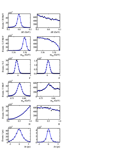
In Fig. 1 we show PDFs for the signal and components for the analysis, which are similar to those for
the analysis. We parameterize the PDFs for the signal
component using simulated events, while the background distributions
are taken from sidebands of the data in the kinematic variables that
exclude signal events. The parameters used in the PDFs are different for
each mode.
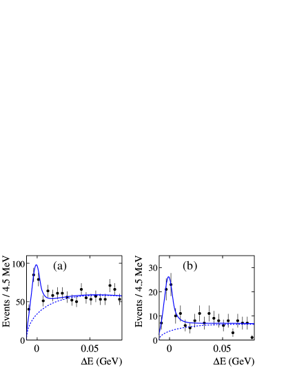
Figure 1: PDFs for ; from top to bottom ,
, , mass, , and . In the left column
we show distributions from signal Monte Carlo; in the right column we show
distributions for the component, which are taken from sidebands of
the data in the kinematic variables that exclude signal events.
For the background PDF shapes we use the following:
the sum of two Gaussians for and ;
a quadratic dependence for , , and ; and the sum of two Gaussians
for .
For and we use
the function
(13)
with ( for ) and a
free parameter Argus , and the same function plus a
Gaussian for and .
For and we use the
function
(14)
where is the peak position of the distribution,
are the left and right widths, and
are the left and right tail parameters.
For in the analysis, we use the function
(15)
where , with fixed to , and
is a free parameter.
To reduce background beyond that obtained with the requirement described above for and (and the
and requirements for ), we use additional event topology
information in the ML fit. The variables used include ,
, , and the angle with respect to the beam axis in the
frame of the signal thrust axis ().
For the analysis, we use and the ratio
directly in the fit, parameterized by a second-order
polynomial and a seven-bin histogram, respectively.
The parameters of the PDF depend on the tagging category
in the signal component. In Fig. 2 we show the PDFs
for signal (background) superimposed on the distribution for data where
background (signal) events are subtracted using an event weighting
technique ref:splots . The bin widths of the histogram have been
adjusted to be coarser where the background is small to reduce the number of
free parameters of the PDF.
Figure 2: Distribution of (a) , (b) , (c) ,
(d) , for signal (background-subtracted) events in data
(points) from the sample.
The solid curve represents the shape of the signal PDF, as
obtained from the ML fit. The insets show the distribution of the data,
and the PDF, for background (signal-subtracted) events.
For the other decay modes we construct a Fisher discriminant , which is an
optimized linear combination of , , , and
. For the modes we also use the continuous
output of the flavor tagging algorithm as a variable entering the
Fisher discriminant. The coefficients used to combine these
variables are chosen to maximize the separation (difference of means
divided by quadrature sum of errors) between the signal and continuum
background distributions of , and are determined from studies of signal
MC and off-peak data. We have studied the optimization of for a variety
of signal modes, and find that a single set of coefficients is
nearly optimal for all.
The PDF shape for is an asymmetric Gaussian with different
widths below and above the peak for signal, plus a broad Gaussian for
background to account for a small tail in the signal region.
The background peak parameter is adjusted to be the same for all tagging
categories . Because describes the overall shape of the event,
the distribution for background is similar to the signal distribution.
For we use the sum of two Gaussians; for
and the
sum of a Gaussian and a quadratic. For
and we use a quadratic dependence,
and for a fourth-order polynomial.
As described in Sec. IV, the resolution function
in
is a sum of three Gaussians for all fit components . For background we use the same functional form as for
signal, but fix the lifetime to zero so that is effectively just the resolution model.
For the signal and background components we determine the parameters of
from simulation, and the background
parameters are free in the final fit. For the signal resolution function
we fix all parameters to values obtained from the sample; we obtain
parameter values from MC for the charm and charmless resolution models;
we leave parameters of the resolution model for free in the final fit.
For the and analyses, we use large control samples to determine any needed adjustments to the
signal PDF shapes that have initially been determined from Monte Carlo. For
and in and , we use the decay with ,
which has similar topology to the modes under study here. We select this
sample by making loose requirements on and , and requiring for
the
candidate mass . We also
place kinematic requirements on the and daughters to force the
charmed decay to look as much like that of a charmless decay as possible.
These selection criteria are applied both to the data and to MC. For
, we use a sample of decays
selected with requirements very similar to those of our signal modes. From
these control samples, we determine small adjustments (of the order of few )
to the mean value of the signal distribution. The means and widths of the other
distributions do not need adjustment.
For the mass line shape, we use production in the data
sidebands. The means and resolutions of the invariant mass
distributions are compared between data and MC, and small adjustments
are made to the PDF parameterizations. These studies also provide
uncertainties in the agreement between data and MC that are used for
evaluation of systematic errors. For the analysis, we apply no
correction to the signal PDF shapes, but we evaluate the related systematic
error as described in Sec. VIII.
VI.3 Fit variables
For the analysis we perform a fit with 25 free
parameters: , , signal yield, continuum background yield and
fractions (6), and the background PDF parameters for , , , ,
, and (15). For the five channels
we perform a single fit with 98 free parameters:
, , signal yields (5), charm background yields (2), continuum background yields (5) and fractions
(30), and the background PDF parameters for , , , and (54).
Similarly the two channels are fit jointly, with parameters:
, , signal yields (2), background yields (2), fractions (12), and
PDF parameters (16). For the
analysis we perform a fit with free parameters: , ,
signal yield, the means of and signal PDFs, background yield, background
PDF parameters for , , , ,
(), background tagging efficiencies (), and the fraction of good
events (). For the signal, charm , and charmless components the
parameters and are fixed to world-average values
PDG2006 ; for the components and are fixed to zero and
then varied to obtain the related systematic uncertainty as described below;
for the model is fixed to zero.
VI.4 Fit validation
We test the fitting procedure by applying it to ensembles
of simulated experiments with and charmed events drawn from
the PDF into which we have embedded the expected number of signal and
charmless background events (with the expected values of and
) randomly extracted from the fully
simulated MC samples. We find biases (measuredexpected) for
, , , , and of
, , , ,
and , respectively.
These small biases are
due to neglected correlations among the observables,
contamination of the signal by self-crossfeed,
and the small signal event yield in . We apply additive
corrections to the final results for these biases. For ,
, and we make no correction but assign a systematic
uncertainty as described in Sec. VIII.
VII Fit results
Table 3: Results of the fits. Signal yields quoted here include events with
no flavor tag information. Subscripts for decay modes denote (1)
, (2) , and (3) .
Mode
# events
Signal yield
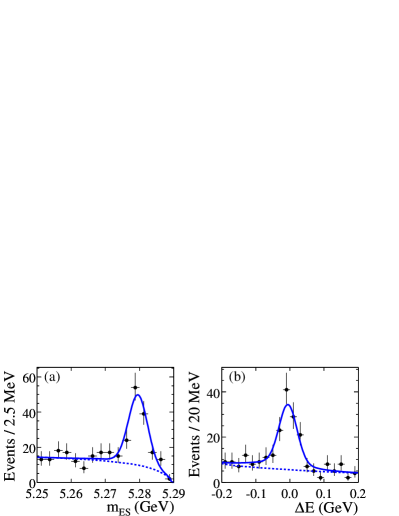
Figure 3: Distributions for projected (see text) onto
(a) and (b) . The solid
lines show the fit result and the dashed lines show the
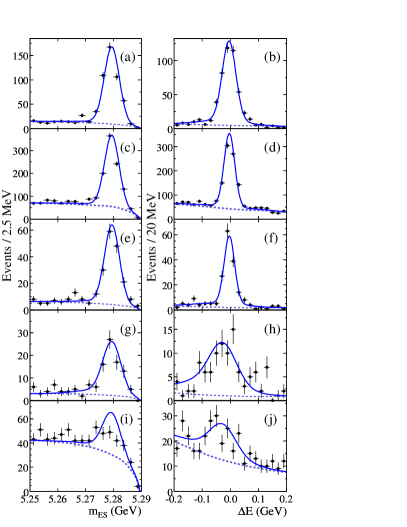
background contributions. Figure 4: Distributions for
(a,b) ,
(c,d) ,
(e,f) ,
(g,h) , and
(i,j)
projected (see text) onto (, ). The solid
lines show the fit result and the dashed lines show the
background contributions.
Results from the fits for the signal yields and the parameters
and are presented in Table 3.
In Figs. 3–9,
we show projections onto the kinematic variables and for subsets of the data for which the
ratio of the likelihood to be signal and the sum of likelihoods to be
signal and background (computed without the variable plotted) exceeds
a mode-dependent threshold that optimizes the statistical significance of
the plotted signal. In the fraction of signal events with
respect to the total after this requirement
has been applied is , while in and , the
fraction of signal events is in the and range
respectively, depending on the decay mode.
In Fig. 3 we show the projections onto and for the analysis; in Fig. 4 we show the
projections onto and for ; in Fig. 5
we show the projections for . The corresponding
information for is conveyed by the background-subtracted
distributions for and in Fig. 2.
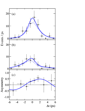
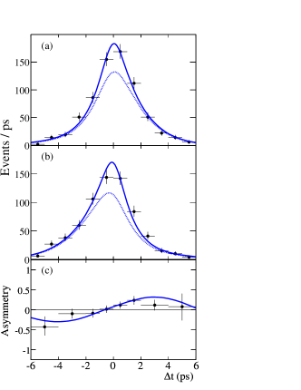
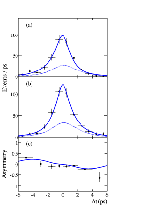
Figure 5: Distributions for (a) and
(b) projected (see
text) onto . The solid lines show the fit result and the dashed
lines show the background contributions. Figure 6: Data and model projections for onto for (a) and (b) tags. We show data as points with error bars and the
total fit function (total signal) with a the solid (dotted) line.
In (c) we show the raw asymmetry,
with a
solid line representing
the fit function.
In Figs. 6–9,
we show the projections and the asymmetry
for each final state.
In the , , ,
and analyses, we measure the correlation between and in
the fit to be 2.9%,
3.0%, 1.0%
and %, respectively.
Figure 7: Data and model projections for onto for (a) and (b) tags. Points with error bars represent the
data; the solid (dotted) line displays the total fit function
(total signal). In (c) we show the raw asymmetry,
; the solid line represents
the fit function.Figure 8: Data and model projections for onto for (a) and (b) tags. Points with error bars represent the
data; the solid (dotted) line displays the total fit function
(total signal). In (c) we show the raw asymmetry,
; the solid line represents
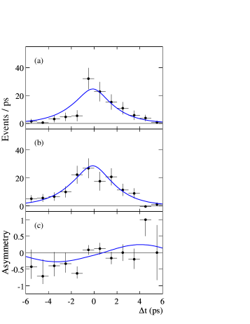
the fit function.Figure 9: Data and model projections for onto for (a) and (b) tags. Points with error bars represent the
signal where backgroud is subtracted using an event weighting
techinque ref:splots ; the solid line displays the signal fit
function. In (c) we show the raw asymmetry,
; the solid line represents
the fit function.
VII.1 Crosschecks
We perform several additional crosschecks of our analysis technique
including time-dependent fits for decays to the final
states , , and
in which measurements of and are
consistent with zero.
There are only small changes in the results when we do any of the following:
fix or , allow and to be different for each tagging
category, remove each of the discriminating variables one by one, and
allow the signal resolution model parameters to vary in the fit.
To validate the IP-constrained vertexing technique in ,
we examine decays in
data where or . In these events
we determine in two ways: by fully reconstructing the
decay vertex using the trajectories of charged daughters of the
and the mesons (standard method), or by neglecting the
contribution to the decay vertex and using the IP constraint
and the trajectory only. This study shows that within
statistical uncertainties
of order 2% of the error on ,
the IP-constrained
measurement is unbiased with respect to the standard technique and
that the fit values of and are consistent
between the two methods.
VIII Systematic uncertainties
A number of sources of systematic uncertainties affecting the fit
values of and have been considered.
We vary the parameters of the signal PDFs that are kept fixed
in the fit within their uncertainty and take as systematic error the
resulting changes of and . These parameters include
and , the mistag parameters and , the
efficiencies of each tagging category, the parameters of the
resolution model, and the shift and scale factors applied to the variables
related to the kinematics and event shape variables that serve to distinguish
signal from background. The deviations of and for and
for variations of and are less than .
For the channel as an additional systematic error
associated with the shape of the PDFs we also use the largest
deviation observed when the parameters of the individual PDFs are
free in the fit.
As a systematic uncertainty related to the fit bias on and we assign
the statistical uncertainty on the bias obtained from simulated experiments
during the fit validation. As explained in Sec. IV, we
obtain parameters of the signal resolution model from a fit to the
sample instead of from a fit to signal MC. We evaluate the
systematic uncertainty of this approach with two sets of simulated experiments
that differ only in the values of resolution model parameters (one set with
parameters from the sample and one set with parameters from MC). We
take the difference in the average and from these two sets of
experiments as the related systematic error.
We evaluate the impact of potential biases arising from
the interference of doubly Cabibbo-suppressed decays with
the Cabibbo-favored decays on the tag-side of the event dcsd
by taking into account realistic values of the ratio between the two
amplitudes and the relative phases.
For and we
estimate using MC, published measurements, and theoretical predictions that
conservative ranges of the net values for parameters in the background are and for the charmless background and
and for the charm background.
We perform a fit in which we
fix the parameters to these values and take the difference in signal parameters between this fit and the nominal fit as the systematic error.
For the and channels we also vary the amount of the charmless
background by . For we do not include a background
component in the fit but we embed background events in the data
sample and extract the peaking background from the observed change in
the yield. We use this yield to estimate the change in and due to the
asymmetry of the peaking background. We also measure the systematic
error associated with the vertex reconstruction by varying within
uncertainties the parameters of the alignment of the SVT and the position
and size of the beam spot.
We quantify the effects of self-crossfeed events in the analysis.
For we perform sets of simulated experiments in which we embed only correctly
reconstructed signal events and compare the results to the nominal simulated
experiments (Sec. VI.4) in which we embed both correctly and
incorrectly reconstructed signal events. We take the difference as the
systematic uncertainty related to self-crossfeed. For the analysis, in which we include a self-crossfeed component in the fit, we
perform a fit in which we take parameter values for the self-crossfeed
resolution model from self-crossfeed MC events instead of the nominal
sample. We take the difference of the results from this fit and the
nominal fit as the self-crossfeed systematic for . The effects of
self-crossfeed are negligible for and .
Table 4: Summary of systematic uncertainties affecting and .
Source
Variation of PDF parameters
0.012
0.019
0.006
0.009
0.009
0.007
0.010
0.012
Bias correction
0.010
0.007
0.006
0.005
0.014
0.009
0.011
0.001
Interference from DCSD on tag side
0.001
0.015
0.001
0.015
0.001
0.015
0.001
0.015
background
0.009
0.010
0.009
0.005
-
-
0.005
0.001
Signal parameters from
0.002
0.001
0.009
0.015
0.004
0.008
0.016
0.011
SVT alignment
0.011
0.003
0.002
0.003
0.004
0.004
0.009
0.009
Beam-spot position and size
0.000
0.000
0.002
0.001
0.004
0.003
0.004
0.002
Vertexing method
-
-
-
-
-
-
0.008
0.016
Self-crossfeed
-
-
0.004
0.001
0.001
0.004
-
-
Total
0.021
0.028
0.016
0.024
0.018
0.021
0.025
0.028
Finally, for the analysis we examine large samples of
simulated and decays to quantify the
differences between resolution function parameter values obtained from
the sample and those of the signal channel; we use these
differences to evaluate uncertainties due to the use of the resolution
function extracted from the sample. We also use the
differences between resolution function parameters extracted from data
and MC in the decays to quantify possible problems in the
reconstruction of the vertex. We take the sum in quadrature of
these errors
as the systematic error related to the vertexing method.
The contributions of the above sources of systematic uncertainties
to and are summarized in Table 4.
IX and parameters for
As noted in Sec. I, the final states and
have opposite eigenvalues, and in the SM, if
, then . We therefore compute the
values of and from our separate measurements with
and , taking in combination with ,
and with .
To represent the results of the individual fits, we project the
likelihood by maximizing (Sec. VI) at a succession of fixed values of to obtain
. We then convolve this likelihood with a
Gaussian function representing the independent systematic errors for each mode.
The product of these convolved one-dimensional likelihood functions for the
two modes, shifted in by their respective corrections (Sec. VI.4), gives the joint likelihood for . The
likelihood for is computed similarly. Since the measured
correlation between and is small in our fits (Sec. VII), we extract the central values and total
uncertainties of these quantities from these one-dimensional likelihood
functions. Applying the same procedure without the convolution over
systematic errors yields the statistical component of the error. The
systematic component is then extracted by subtraction in quadrature from
the total error.
X Summary and discussion
In conclusion, we have used samples of
,
,
, and
flavor-tagged events to measure the time-dependent violation
parameters
where the first errors are statistical and the second systematic.
These results are consistent with and supersede our previous measurements
PreviousOmK ; PreviousEtapK ; PreviousPizK ;
they are also consistent with the world average of measured in PDG2006 .
XI Acknowledgements
We are grateful for the
extraordinary contributions of our PEP-II colleagues in
achieving the excellent luminosity and machine conditions
that have made this work possible.
The success of this project also relies critically on the
expertise and dedication of the computing organizations that
support BABAR.
The collaborating institutions wish to thank
SLAC for its support and the kind hospitality extended to them.
This work is supported by the
US Department of Energy
and National Science Foundation, the
Natural Sciences and Engineering Research Council (Canada),
the Commissariat à l’Energie Atomique and
Institut National de Physique Nucléaire et de Physique des Particules
(France), the
Bundesministerium für Bildung und Forschung and
Deutsche Forschungsgemeinschaft
(Germany), the
Istituto Nazionale di Fisica Nucleare (Italy),
the Foundation for Fundamental Research on Matter (The Netherlands),
the Research Council of Norway, the
Ministry of Education and Science of the Russian Federation,
Ministerio de Educación y Ciencia (Spain), and the
Science and Technology Facilities Council (United Kingdom).
Individuals have received support from
the Marie-Curie IEF program (European Union) and
the A. P. Sloan Foundation.
References
(1)BABAR Collaboration, B. Aubert et al., Phys. Rev. Lett. 89, 201802 (2002);
Belle Collaboration, K. Abe et al., Phys. Rev. D 66, 071102(R) (2002).
(2)N. Cabibbo, Phys. Rev. Lett. 10, 531 (1963); M. Kobayashi and T. Maskawa, Prog. Theor. Phys. 49, 652 (1973).
(3)Y. Grossman and M. P. Worah, Phys. Lett. B 395, 241 (1997);
D. Atwood and A. Soni, Phys. Lett. B 405, 150 (1997);
M. Ciuchini et al., Phys. Rev. Lett. 79, 978 (1997).
(4) M. Beneke and M. Neubert, Nucl. Phys. B 675, 333 (2003).
(5)C.-W. Chiang, M. Gronau, and J. L. Rosner, Phys. Rev. D 68, 074012 (2003); M. Gronau, J. L. Rosner, and J. Zupan, Phys. Lett. B 596, 107 (2004).
(6) D. London and A. Soni, Phys. Lett. B 407, 61 (1997).
(7) Y. Grossman, Z. Ligeti, Y. Nir, and H. Quinn, Phys. Rev. D 68, 015004 (2003).
(8) M. Beneke, Phys. Lett. B 620, 143 (2005).
(9) H. Y. Cheng, C-K. Chua, and A. Soni, Phys. Rev. D 72, 014006 (2005), Phys. Rev. D 71,
014030 (2005); S. Fajfer, T. N. Pham, and A. Prapotnik-Brdnik Phys. Rev. D 72, 114001 (2005).
(10) A. R. Williamson and J. Zupan, Phys. Rev. D 74, 014003 (2006).
(11) M. Gronau, J. L. Rosner, and J. Zupan, Phys. Rev. D 74, 093003 (2006).
(12) H-Y. Cheng, C-K. Chua, and A. Soni, Phys. Rev. D 72, 014006 (2005).
(13) A. J. Buras, R. Fleischer, S. Recksiegel, and F. Schwab, Phys. Rev. Lett. 92, (2004) 101804; R. Fleischer, S. Jager, D. Pirjol, and J. Zupan,
Phys. Rev. D 78, 111501 (2008); M. Gronau and J. L. Rosner, Phys. Lett. B 666, 467 (2008).
(14)BABAR Collaboration, B. Aubert et al., Phys. Rev. D 74, 011106 (2006).
(15)BABAR Collaboration, B. Aubert et al., Phys. Rev. Lett. 98, 031801 (2007).
(16)BABAR Collaboration , B. Aubert et al., Phys. Rev. D 77, 012003 (2008).
(17)
Belle Collaboration, K. Abe et al., Phys. Rev. Lett. 98, 031802 (2007).
(18)
Belle Collaboration, K. F. Chen et al., Phys. Rev. D 76, 091103 (2007).
(19)BABAR Collaboration, B. Aubert et al., Nucl. Instrum. Methods Phys. Res., Sect. A 479, 1 (2002).
(20)
G. Benelli et al., Nuclear Science Symposium
Conference Record, 2005 IEEE, 2, 1145 (2005).
(21)BABAR Collaboration, B. Aubert et al., Phys. Rev. Lett. 93, 131805 (2004).
(22)BABAR Collaboration, B. Aubert et al., Phys. Rev. D 66, 032003 (2002).
(23)
S. Agostinelli et al., Nucl. Instrum. Methods Phys. Res., Sect. A 506, 250 (2003).
(24)BABAR Collaboration, B. Aubert et al., Phys. Rev. D 66, 032003 (2002).
(25)
Particle Data Group, Y.-M. Yao et al., J. Phys. G33, 1 (2006).
(26)BABAR Collaboration, B. Aubert et al., Phys. Rev. D 71,
111102 (2005).
(27)
A. de Rújula, J. Ellis, E. G. Floratos, and M. K. Gaillard,
Nucl. Phys. B 138, 387 (1978).
(28)
ARGUS Collaboration, H. Albrecht et al., Phys. Lett. B 241, 278 (1990).
(29)
M. Pivk and F. R. Le Diberder,
Nucl. Instrum. Methods Phys. Res., Sect. A 555, 356 (2005).
(30)
O. Long, M. Baak, R. N. Cahn, and D. Kirkby, Phys. Rev. D 68, 034010 (2003).