Minkowski Sum Selection and Finding

Abstract

Let $P,Q\subseteq{\mathbb{R}^{2}}$ be two $n$-point multisets and $Ar\geq b$ be a set of $\lambda$ inequalities on $x$ and $y$, where $A\in\mathbb{R}^{\lambda\times 2}$, $r=[^{x}_{y}]$, and $b\in\mathbb{R}^{\lambda}$. Define the constrained Minkowski sum $(P\oplus Q)_{Ar\geq b}$ as the multiset $\{(p+q)|p\in P,q\in Q,A(p+q)\geq b\}$. Given $P$, $Q$, $Ar\geq b$, an objective function $f:\mathbb{R}^{2}\rightarrow\mathbb{R}$, and a positive integer $k$, the Minkowski Sum Selection problem is to find the $k^{th}$ largest objective value among all objective values of points in $(P\oplus Q)_{Ar\geq b}$. Given $P$, $Q$, $Ar\geq b$, an objective function $f:\mathbb{R}^{2}\rightarrow\mathbb{R}$, and a real number $\delta$, the Minkowski Sum Finding problem is to find a point $(x^{*},y^{*})$ in $(P\oplus Q)_{Ar\geq b}$ such that $|f(x^{*},y^{*})-\delta|$ is minimized. For the Minkowski Sum Selection problem with linear objective functions, we obtain the following results: (1) optimal $O(n\log n)$ time algorithms for $\lambda=1$; (2) $O(n\log^{2}n)$ time deterministic algorithms and expected $O(n\log n)$ time randomized algorithms for any fixed $\lambda>1$. For the Minkowski Sum Finding problem with linear objective functions or objective functions of the form $f(x,y)=\frac{by}{ax}$, we construct optimal $O(n\log n)$ time algorithms for any fixed $\lambda\geq 1$. As a byproduct, we obtain improved algorithms for the Length-Constrained Sum Selection problem and the Density Finding problem.

Keywords. Bioinformatics, Sequence analysis, Minkowski sum.

1 Introduction

Let $P,Q\subseteq{\mathbb{R}^{2}}$ be two $n$-point multisets and $Ar\geq b$ be a set of $\lambda$ inequalities on $x$ and $y$, where $A\in\mathbb{R}^{\lambda\times 2}$, $r=[^{x}_{y}]$, and $b\in\mathbb{R}^{\lambda}$. Define the constrained Minkowski sum $(P\oplus Q)_{Ar\geq b}$ as the multiset $\{(p+q)|p\in P,q\in Q,A(p+q)\geq b\}.$

In the Minkowski Sum Optimization problem, we are given $P$, $Q$, $Ar\geq b$, and an objective function $f:\mathbb{R}^{2}\rightarrow\mathbb{R}$. The goal is to find the maximum objective value among all objective values of points in $(P\oplus Q)_{Ar\geq b}$. A function $f:D\subseteq\mathbb{R}^{2}\rightarrow\mathbb{R}$ is said to be quasiconvex if and only if for all points $v_{1},v_{2}\in D$ and all $\gamma\in[0,1]$, one has $f(\gamma\cdot v_{1}+(1-\gamma)\cdot v_{2})\leq\max(f(v_{1}),f(v_{2}))$. Bernholt et al. [5] studied the Minkowski Sum Optimization problem for quasiconvex objective functions and showed that their results have applications to many optimization problems arising in computational biology [1, 6, 9, 10, 15, 16, 17, 21]. In this paper, two variations of the Minkowski Sum Optimization problem are studied: the Minkowski Sum Selection problem and the Minkowski Sum Finding problem.

In the Minkowski Sum Selection problem, we are given $P$, $Q$, $Ar\geq b$, an objective function $f:\mathbb{R}^{2}\rightarrow\mathbb{R}$, and a positive integer $k$. The goal is to find the $k^{th}$ largest objective value among all objective values of points in $(P\oplus Q)_{Ar\geq b}$. The Minkowski Sum Optimization problem is equivalent to the Minkowski Sum Selection problem with $k=1$. A variety of selection problems, including the Sum Selection problem [3, 13], the Length-Constrained Sum Selection problem [14], and the Slope Selection problem [7, 18], are linear-time reducible to the Minkowski Sum Selection problem with a linear objective function or an objective function of the form $f(x,y)=\frac{by}{ax}$. It is desirable that relevant selection problems from diverse fields are integrated into a single one, so we don’t have to consider them separately. Next, let us look at the use of the Minkowski Sum Selection problem in practice. As mentioned above, the Minkowski Sum Optimization problem finds applications to many optimization problems arising in computational biology [1, 6, 9, 10, 15, 16, 17, 21]. In these optimization problems, the objective functions are chosen such that feasible solutions with higher objective values are “more likely” to be biologically meaningful. However, it is not guaranteed that the best feasible solution always satisfies the needs of biologists. If the best feasible solution does not interest biologists or does not provide enough information, we still have to find the second best feasible solution, the third best feasible solution and so on until a satisfying feasible solution is finally found. As a result, it is desirable to know how to dig out extra good feasible solutions in case that the best feasible solution is not sufficient.

In the Minkowski Sum Finding problem, we are given $P$, $Q$, $Ar\geq b$, an objective function $f:\mathbb{R}^{2}\rightarrow\mathbb{R}$, and a real number $\delta$. The goal is to find a point $(x^{*},y^{*})$ in $(P\oplus Q)_{Ar\geq b}$ such that $|f(x^{*},y^{*})-\delta|$ is minimized. This problem originates from the study of the Density Finding problem proposed by Lee $et~{}al.$ [12]. The Density Finding problem can be regarded as a specialization of the Minkowski Sum Finding problem with objective function $f(x,y)=\frac{y}{x}$ and find applications in recognizing promoters in DNA sequences [11, 20]. In these applications, the goal is not to find the feasible solution with the highest objective value. Instead, feasible solutions with objective values close to some specific number, say $\delta$, are thought to be more biologically meaningful and preferred.

The main results obtained in this paper are as follows.

• The Minkowski Sum Selection problem with one constraint and a linear objective function can be solved in optimal $O(n\log n)$ time.

• The Minkowski Sum Selection problem with two constraints and a linear objective function can be solved in $O(n\log^{2}n)$ time by a deterministic algorithm and expected $O(n\log n)$ time by a randomized algorithm.

• For any fixed $\lambda>2$, the Minkowski Sum Selection problem with $\lambda$ constraints and a linear objective function is shown to be asymptotically equivalent to the Minkowski Sum Selection problem with two constraints and a linear objective function.

• The Minkowski Sum Finding problem with any fixed number of constraints can be solved in optimal $O(n\log n)$ time if the objective function $f(x,y)$ is linear or of the form $\frac{by}{ax}$.

As a byproduct, we obtain improved algorithms for the Length-Constrained Sum Selection problem [14] and the Density Finding problem [12]. Recently, Lin and Lee [14] proposed an expected $O(n\log(u-l+1))$-time randomized algorithm for the Length-Constrained Sum Selection problem, where $n$ is the size of the input instance and $l,u\in\mathbb{N}$ are two given parameters with $1\leq l<u\leq n$. In this paper, we obtain a worst-case $O(n\log(u-l+1))$-time deterministic algorithm for the Length-Constrained Sum Selection problem (see Appendix A). Lee, Lin, and Lu [12] showed the Density Finding problem has a lower bound of $\Omega(n\log n)$ and proposed an $O(n\log^{2}m)$-time algorithm for it, where $n$ is the size of the input instance and $m$ is a parameter whose value may be as large as $n$. In this paper, we give an optimal $O(n\log n)$-time algorithm for the Density Finding problem (see Appendix B).

2 Preliminaries

In the following, we review some definitions and theorems. For more details, readers can refer to [5, 8]. A matrix $X\in\mathbb{R}^{\mathfrak{n}\times\mathfrak{m}}$ is said to be sorted if the values of each row and each column are in nondecreasing order. Frederickson and Johnson [8] gave some results about the selection problem and the ranking problem in a collection of sorted matrices. From the results of Frederickson and Johnson [8], we have the following theorems.

Theorem 1

: The selection problem in a collection of sorted matrices is given a rank $k$ and a collection of sorted matrices $\{X_{1},\ldots,X_{N}\}$ in which $X_{j}$ has dimensions $n_{j}\times m_{j}$, $n_{j}\geq m_{j}$, to find the $k^{th}$ largest element among all elements of sorted matrices in $\{X_{1},\ldots,X_{N}\}$. This problem is able to be solved in $O(\sum_{j=1}^{N}m_{j}\log(2n_{j}/m_{j}))$ time.

Theorem 2

: The ranking problem in a collection of sorted matrices is given an element and a collection of sorted matrices $\{X_{1},\ldots,X_{N}\}$ in which $X_{j}$ has dimensions $n_{j}\times m_{j}$, $n_{j}\geq m_{j}$, to find the rank of the given element among all elements of sorted matrices in $\{X_{1},\ldots,X_{N}\}$. This problem can be solved in $O(\sum_{j=1}^{N}m_{j}\log(2n_{j}/m_{j}))$ time.

By the recent works of Bernholt et al. [5], we have the following theorems.

Theorem 3

: Given a set of $\lambda$ linear inequalities $Ar\geq b$ and two $n$-point multisets $P$, $Q\subseteq{\mathbb{R}^{2}}$, one can compute the vertices of the convex hull of $(P\oplus Q)_{Ar\geq b}$ in $O(\lambda\log\lambda+\lambda\cdot n\log n)$ time.

Theorem 4

: The problem of maximizing a quasiconvex objective function $f$ over the constrained Minkowski sum $(P\oplus Q)_{Ar\geq b}$ requires $\Omega(n\log n)$ time in the algebraic decision tree model even if $f$ is a linear function and $Ar\geq b$ consists of only one constraint.

3 Minkowski Sum Selection with One Constraint

In this section we study the Minkowski Sum Selection problem and give an optimal $O(n\log n)$ time algorithm for the case where only one linear constraint is given and the objective function is also linear.

3.1 Input Transformation

Given $P=\{(x_{1,1},y_{1,1}),\ldots,(x_{1,n},y_{1,n})\}$, $Q=\{(x_{2,1},y_{2,1}),\ldots,(x_{2,n},y_{2,n})\}$, a positive integer $k$, one constraint $L$: $ax+by\geq c$, and a linear objective function $f(x,y)=dx+ey$, where $a$, $b$, $c$, $d$, and $e$ are all constants, we perform the following transformation.

1. Change the content of $P$ and $Q$ to $\{(ax_{1,1}+by_{1,1},dx_{1,1}+ey_{1,1}),\ldots,(ax_{1,n}+by_{1,n},dx_{1,n}+ey_{1,n})\}$, and $\{(ax_{2,1}+by_{2,1},dx_{2,1}+ey_{2,1}),\ldots,(ax_{2,n}+by_{2,n},dx_{2,n}+ey_{2,n})\}$, respectively.

2. Change the constraint from $ax+by\geq c$ to $x\geq c$.

3. Change the objective function from $dx+ey$ to $y$.

This transformation can be done in $O(n)$ time and the answer remains the same. Hence from now on, our goal becomes to find the $k^{th}$ largest $y$-coordinate on the constrained Minkowski sum of $P$ and $Q$ subject to the constraint $L:x\geq c$.

3.2 Algorithm

For ease of exposition, we assume that no two points in $P$ and $Q$ have the same $x$-coordinate and $n$ is a power of two. The algorithm proceeds as follows. First, we sort $P$ and $Q$ into $P_{x}$ and $Q_{x}$ ($P_{y}$ and $Q_{y}$, respectively) in nondecreasing order of $x$-coordinates ($y$-coordinates, respectively) in $O(n\log n)$ time. Next, we use a divide-and-conquer approach to store the $y$-coordinates of $(P\oplus Q)_{x\geq c}$ as a collection of sorted matrices and then apply Theorem 1 to select the $k^{th}$ largest element from the elements of these sorted matrices.

Now we explain how to store the $y$-coordinates of $(P\oplus Q)_{x\geq c}$ as a collection of sorted matrices. Let $P_{x}=((x_{1},y_{1}),\ldots,(x_{n},y_{n}))$, $Q_{x}=((\bar{x}_{1},\bar{y_{1}}),\ldots,(\bar{x}_{n},\bar{y}_{n}))$, $P_{y}=((x^{\prime}_{1},y^{\prime}_{1}),\ldots,(x^{\prime}_{n},y^{\prime}_{n})),$ and $Q_{y}=((\bar{x}^{\prime}_{1},\bar{y}^{\prime}_{1}),\ldots,(\bar{x}^{\prime}_{n},\bar{y}^{\prime}_{n})).$ We then divide $P_{x}$ into two halves of equal size: $A=((x_{1},y_{1}),\ldots,(x_{n/2},y_{n/2}))$ and $B=((x_{n/2+1},y_{n/2+1}),\ldots,(x_{n},y_{n})).$ Find a point $(\bar{x}_{t},\bar{y}_{t})$ of $Q_{x}$ such that $x_{n/2}+\bar{x}_{t}<c$ and $t$ is maximized. Then divide $Q_{x}$ into two halves: $C=((\bar{x}_{1},\bar{y}_{1}),\ldots,(\bar{x}_{t},\bar{y}_{t}))$ and $D=((\bar{x}_{t+1},\bar{y}_{t+1}),\ldots,(\bar{x}_{n},\bar{y}_{n})).$ The set $(P\oplus Q)_{x\geq c}$ is the union of $(A\oplus C)_{x\geq c}$, $(A\oplus D)_{x\geq c}$, $(B\oplus C)_{x\geq c}$, and $(B\oplus D)_{x\geq c}$. Because $\bar{x}_{t}$ is the largest $x$-coordinate among all $x$-coordinates of points in $Q_{x}$ such that $x_{n/2}+\bar{x}_{t}<c$, we know that all points in $A\oplus C$ cannot satisfy the constraint $x\geq c$. Hence, we only need to consider points in $A\oplus D$, $B\oplus C$, and $B\oplus D$. Because $P_{x}$ and $Q_{x}$ are in nondecreasing order of $x$-coordinates, it is guaranteed that all points in $B\oplus D$ satisfy the constraint $L$, i.e., $B\oplus D=(B\oplus D)_{x\geq c}$. Construct in linear time row_vector = $(r_{1},r_{2},\ldots,r_{n/2})$ which is the $y$-coordinates in the subsequence of $P_{y}$ resulting from removing points with $x$-coordinates no greater than $x_{n/2}$ from $P_{y}$. Construct in linear time column_vector = $(c_{1},c_{2},\ldots,c_{n-t})$ which is the $y$-coordinates in the subsequence of $Q_{y}$ resulting from removing points with $x$-coordinates no greater than $\bar{x}_{t}$ from $Q_{y}$. Note row_vector is the same as the result of sorting $B$ into nondecreasing order of $y$-coordinates, and column_vector is the same as the result of sorting $D$ into nondecreasing order of $y$-coordinates. Thus, we have $\{y:(x,y)\in(B\oplus D)_{x\geq c}\}=\{y:(x,y)\in B\oplus D\}=\{r_{i}+c_{j}:1\leq i\leq|row\_vector|,1\leq j\leq|column\_vector|\}$. Therefore, we can store the $y$-coordinates of $B\oplus D=(B\oplus D)_{x\geq c}$ as a sorted matrix $X$ of dimensions $|row\_vector|\times|column\_vector|$ where the $(i,j)$-th element of $X$ is $r_{i}+c_{j}$. Note that it is not necessary to explicitly construct the sorted matrix $X$, which needs $\Omega(n^{2})$ time. Because the $(i,j)$-th element of $X$ can be obtained by summing up $r_{i}$ and $c_{j}$, we only need to keep $row\_vector$ and $column\_vector$. The rest is to construct the sorted matrices for the $y$-coordinates of points in $(A\oplus D)_{x\geq c}$ and $(B\oplus C)_{x\geq c}$. It is accomplished by applying the above approach recursively. The pseudocode is shown in Figure 1 and Figure 2. We now analyze the time complexity.

Algorithm ConstructMatrices$(P_{x},Q_{x},P_{y},Q_{y},L$: $x\geq c)$
Input: $P_{x}$ and $P_{y}$ are the results of sorting the multiset $P\subseteq\mathbb{R}^{2}$ in nondecreasing
	order of $x$-coordinates and $y$-coordinates, respectively. $Q_{x}$ and $Q_{y}$ are the results
	of sorting the multiset $Q\subseteq\mathbb{R}^{2}$ in nondecreasing order of $x$-coordinates and
	$y$-coordinates, respectively. A linear constraint $L$: $x\geq c$.
Output: The $y$-coordinates of points in $(P\oplus Q)_{x\geq c}$ as a collection of sorted matrices.
1	$n^{\prime}\leftarrow|P_{x}|$; $m^{\prime}\leftarrow|Q_{x}|$.
2	Let $P_{x}=((x_{1},y_{1}),\ldots,(x_{n^{\prime}},y_{n^{\prime}}))$, $Q_{x}=((\bar{x}_{1},\bar{y_{1}}),\ldots,(\bar{x}_{m^{\prime}},\bar{y}_{m^{\prime}}))$,
	$P_{y}=((x^{\prime}_{1},y^{\prime}_{1}),\ldots,(x^{\prime}_{n^{\prime}},y^{\prime}_{n^{\prime}})),$ and $Q_{y}=((\bar{x}^{\prime}_{1},\bar{y}^{\prime}_{1}),\ldots,(\bar{x}^{\prime}_{m^{\prime}},\bar{y}^{\prime}_{m^{\prime}})).$
3	$\bar{x}_{0}\leftarrow-\infty$.
4	if $n^{\prime}\leq 0$ or $m^{\prime}\leq 0$ then
5  return
6	if $n^{\prime}=1$ or $m^{\prime}=1$ then
7  Scan points in $P_{x}\oplus Q_{x}$ to find all points satisfying $L$ and construct the sorted
matrix for $y$-coordinates of these points.
8  return the above sorted matrix.
9	for $t\leftarrow m^{\prime}$ down to $0$ do
10  if $x_{n^{\prime}/2}+\bar{x}_{t}<c$ then
11		row_vector $\leftarrow$ subsequence of $P_{y}$ being removed points with
		$x$-coordinates $\leq x_{n^{\prime}/2}$.
12		column_vector $\leftarrow$ subsequence of $Q_{y}$ being removed points with
		$x$-coordinates $\leq\bar{x}_{t}$.
13		$A_{x}\leftarrow P_{x}[1,n^{\prime}/2]$; $B_{x}\leftarrow P_{x}[n^{\prime}/2+1,n^{\prime}]$; $C_{x}\leftarrow Q_{x}[1,t]$; $D_{x}\leftarrow Q_{x}[t+1,m^{\prime}]$.
14		$A_{y}\leftarrow$ subsequence of $P_{y}$ being removed points with $x$-coordinates $>x_{n^{\prime}/2}$.
15		$B_{y}\leftarrow$ subsequence of $P_{y}$ being removed points with $x$-coordinates $\leq x_{n^{\prime}/2}$.
16		$C_{y}\leftarrow$ subsequence of $Q_{y}$ being removed points with $x$-coordinates $>\bar{x}_{t}$.
17		$D_{y}\leftarrow$ subsequence of $Q_{y}$ being removed points with $x$-coordinates $\leq\bar{x}_{t}$.
18		ConstructMatrices($A_{x},D_{x},A_{y},D_{y},L$: $x\geq c$).
19		ConstructMatrices($B_{x},C_{x},B_{y},C_{y},L$: $x\geq c$).
20		return row_vector and column_vector.

Figure 1: The subroutine for the Minkowski Sum Selection problem with one linear constraint and a linear objective function.

Algorithm Selection${}_{1}(P,Q,L,f,k)$
Input: Two multisets $P\subseteq\mathbb{R}^{2}$ and $Q\subseteq\mathbb{R}^{2}$; a linear constraint $L$; a linear objective
	function $f:{\mathbb{R}^{2}}\rightarrow\mathbb{R}$; a positive integer $k$.
Output: The $k^{th}$ largest value among all objective values of points in $(P\oplus Q)_{L}$.
1	Perform the input transformation described in Section 3.1.
2	Sort $P$ and $Q$ into $P_{x}$ and $Q_{x}$, respectively, in nondecreasing order of $x$-coordinates.
3	Sort $P$ and $Q$ into $P_{y}$ and $Q_{y}$, respectively, in nondecreasing order of $y$-coordinates.
4	$S\leftarrow$ ConstructMatrices$(P_{x},Q_{x},P_{y},Q_{y},L)$.
5	return the $k^{th}$ largest element among the elements of sorted matrices in $S.$

Figure 2: The main procedure for the Minkowski Sum Selection problem with one linear constraint and a linear objective function.

Lemma 1

: Given a matrix $X\in\mathbb{R}^{\mathfrak{N}\times\mathfrak{M}}$, we define the side length of $X$ be $\mathfrak{N}+\mathfrak{M}$. Letting $T(n^{\prime},m^{\prime})$ be the running time of ConstructMatrices($P_{x},Q_{x},P_{y},Q_{y},L$), where $n^{\prime}=|P_{x}|=|P_{y}|$ and $m^{\prime}=|Q_{x}|=|Q_{y}|$, we have $T(n^{\prime},m^{\prime})=O((n^{\prime}+m^{\prime})\log(n^{\prime}+1)).$ Similarly, letting $M(n^{\prime},m^{\prime})$ be the sum of the side lengths of all sorted matrices created by running ConstructMatrices($P_{x},Q_{x},P_{y},Q_{y},L$), we have $M(n^{\prime},m^{\prime})=O((n^{\prime}+m^{\prime})\log(n^{\prime}+1)).$

Proof: It suffices to prove that $T(n^{\prime},m^{\prime})=O((n^{\prime}+m^{\prime})\log(n^{\prime}+1)).$ By Algorithm ConstructMatrices in Figure 1, we have $T(n^{\prime},m^{\prime})\leq\max_{0\leq i\leq m^{\prime}}\{c^{\prime}(n^{\prime}+m^{\prime})+T(n^{\prime}/2,i)+T(n^{\prime}/2,m^{\prime}-i)\}\mbox{ for some constant }c^{\prime}.$ Then by induction on $n^{\prime}$, it is easy to prove that $T(n^{\prime},m^{\prime})$ is $O((n^{\prime}+m^{\prime})\log(n^{\prime}+1))$.      

Theorem 5

: Given two $n$-point multisets $P\subseteq\mathbb{R}^{2}$ and $Q\subseteq\mathbb{R}^{2}$, a positive integer $k$, a linear constraint $L$, and a linear objective function $f:\mathbb{R}^{2}\rightarrow\mathbb{R}$, Algorithm Selection₁ finds the $k^{th}$ largest objective value among all objective values of points in $(P\oplus Q)_{L}$ in $O(n\log n)$ time. Hence, by Theorem 4, Algorithm Selection₁ is optimal.

Proof: Let $S=\{X_{1},\ldots,X_{N}\}$ be the sorted matrices produced at Step 4 in Algorithm Selection₁. Let $X_{j}$, $1\leq j\leq N$, be of dimensions $n_{j}\times m_{j}$ where $n_{j}\geq m_{j}$. By Lemma 1, we have $O(\sum_{i=1}^{N}(m_{i}+n_{i}))=O(n\log n).$ By Theorem 1, the time required to find the $k^{th}$ largest element from the elements of matrices in $S$ is $O(\sum_{i=1}^{N}m_{i}\log(2n_{i}/m_{i}))$. Since

$$\sum_{i=1}^{N}m_{i}\log(2n_{i}/m_{i})\leq\sum_{i=1}^{N}m_{i}\frac{2n_{i}}{m_{i}}=\sum_{i=1}^{N}2n_{i}\leq\sum_{i=1}^{N}2(m_{i}+n_{i})=O(n\log n),$$

the time for selecting the $k^{th}$ largest element from elements of matrices in $S$ is $O(n\log n)$. Combining this with the time for the input transformation, sorting, and executing ConstructMatrices($P_{x},Q_{x},P_{y},Q_{y},L$), we conclude that the total running time is $O(n\log n)$.      

Using similar techniques, the following problem can also be solved in $O(n\log n)$ time. Given two $n$-point multisets $P\subseteq\mathbb{R}^{2}$ and $Q\subseteq\mathbb{R}^{2}$, a linear constraint $L$, a linear objective function $f:\mathbb{R}^{2}\rightarrow\mathbb{R}$, and a real number $t$, the problem is to find the rank of $t$ among all objective values of points in $(P\oplus Q)_{L}$, where the rank of $t$ is equal to the number of elements in $\{y|(x,y)\in(P\oplus Q)_{L},y>t\}$ plus one. The pseudocode is given in Figure 3. Note that in Algorithm Selection₁ and Algorithm Ranking₁, we assume the input constraint is of the form $ax+by\geq c$. After slight modifications, we can also cope with constraints of the form $ax+by>c$. To avoid redundancy, we omit the details here. For ease of exposition, we assume that Algorithm Selection₁ and Algorithm Ranking₁ are also capable of coping with constraints of the form $ax+by>c$ in the following sections.

Algorithm Ranking${}_{1}(P,Q,L,f,t)$
Input: Two multisets $P\subseteq\mathbb{R}^{2}$ and $Q\subseteq\mathbb{R}^{2}$; a linear constraint $L$; a linear objective
	function $f:{\mathbb{R}^{2}}\rightarrow\mathbb{R}$; a real number $t$.
Output: The rank of $t$ among the objective values of points in $(P\oplus Q)_{L}$.
1	Perform the input transformation in Section 3.1.
2	Sort $P$ and $Q$ into $P_{x}$ and $Q_{x}$, respectively, in nondecreasing order of $x$-coordinates.
3	Sort $P$ and $Q$ into $P_{y}$ and $Q_{y}$, respectively, in nondecreasing order of $y$-coordinates.
4	$S\leftarrow$ ConstructMatrices$(P_{x},Q_{x},P_{y},Q_{y},L)$.
5	return the rank of $t$ among the elements of sorted matrices in $S.$

Figure 3: The ranking algorithm for the Minkowski sum with one linear constraint and a linear objective function.

4 Minkowski Sum Selection with Two Constraints

In this section, we show the Minkowski Sum Selection problem can be solved in worst-case $O(n\log^{2}n)$ time and expected $O(n\log n)$ time for the case where two linear constraints are given and the objective function is linear.

4.1 Input Transformation.

Given $P=\{(x_{1,1},y_{1,1}),\ldots,(x_{1,n},y_{1,n})\}$, $Q=\{(x_{2,1},y_{2,1}),\ldots,(x_{2,n},y_{2,n})\}$, a positive integer $k$, two constraints $L_{1}$: $a_{1}x+b_{1}y\geq c_{1}$ and $L_{2}$: $a_{2}x+b_{2}y\geq c_{2}$, and a linear objective function $f(x,y)=dx+ey$, where $a_{1}$, $b_{1}$, $c_{1}$, $a_{2}$, $b_{2}$, $c_{2}$, $d$, and $e$ are all constants, we perform the following transformation.

1. Change the content of $P$ and $Q$ to $\{(a_{1}x_{1,1}+b_{1}y_{1,1},dx_{1,1}+ey_{1,1}),\ldots,(a_{1}x_{1,n}+b_{1}y_{1,n},dx_{1,n}+ey_{1,n})\}$, and $\{(a_{1}x_{2,1}+b_{1}y_{2,1},dx_{2,1}+ey_{2,1}),\ldots,(a_{1}x_{2,n}+b_{1}y_{2,n},dx_{2,n}+ey_{2,n})\}$, respectively.

2. Change the constraints from $a_{1}x+b_{1}y\geq c_{1}$ and $a_{2}x+b_{2}y\geq c_{2}$ to $x\geq c_{1}$ and $\frac{a_{2}e-b_{2}d}{a_{1}e-b_{1}d}x+\frac{a_{1}b_{2}-b_{1}a_{2}}{a_{1}e-b_{1}d}y\geq c_{2}$, respectively.

3. Change the objective function from $dx+ey$ to $y$.

This transformation can be done in $O(n)$ time and the answer remains the same. Hence from now on, our goal becomes to find the $k^{th}$ largest $y$-coordinate on the constrained Minkowski sum of $P$ and $Q$ subject to the constraints $L_{1}$: $x\geq c_{1}$ and $L_{2}$: $ax+by\geq c_{2}$, where $a=\frac{a_{2}e-b_{2}d}{a_{1}e-b_{1}d}$ and $b=\frac{a_{1}b_{2}-b_{1}a_{2}}{a_{1}e-b_{1}d}.$ Note that if the two constraints and the objective function are parallel, we cannot use the above transformation. However, if the two constraints are parallel, this problem can be solved in $O(n\log n)$ time. For the space limitation, we present the algorithm for this special case in Appendix C.

4.2 Algorithm

After applying the above input transformation to our problem instances, there are four possible cases: (1) $a<0,b<0$; (2) $a>0,b>0$; (3) $a<0,b>0$; (4) $a>0,b<0$. Note that the two constraints are not parallel implies $b\neq 0$. If $a=0$, we can solve this case more easily in $O(n\log^{2}n)$ time by using the same technique stated later and we omit the details here. In the following discussion we focus on Case (1), and the other three cases can be solved in a similar way.

For simplicity, we assume that $n$ is a power of two, and each point in $(P\oplus Q)_{L_{1},L_{2}}$ has a distinct $y$-coordinate. Now we are ready to describe our algorithm. First, we sort $P$ and $Q$ into $P_{y}$ and $Q_{y}$, respectively, in nondecreasing order of $y$-coordinates using $O(n\log n)$ time. Let $P_{y}=\{(x^{\prime}_{1},y^{\prime}_{1}),\ldots,(x^{\prime}_{n},y^{\prime}_{n})\}$ and $Q_{y}=\{(\bar{x}^{\prime}_{1},\bar{y}^{\prime}_{1}),\ldots,(\bar{x}^{\prime}_{n},\bar{y}^{\prime}_{n})\}$. Denote by $Y$ the sorted matrix of dimensions $n\times n$ where the $(i,j)$-th element is $y^{\prime}_{i}+\bar{y}^{\prime}_{j}$. We then run a loop where an integer interval $[l,u]$ is maintained such that the solution is within the set $\{\mbox{the }h^{th}\mbox{ largest element of }Y:l\leq h\leq u\}$. Initially, we set $l=1$ and $u=n^{2}$. At the beginning of each iteration, we select the $\frac{u-l+1}{2}$-th largest element $t$ of $Y$, which can be done in $O(n)$ time by Theorem 1. Let $R$ be the rank of $t$ among the objective values of points in $(P\oplus Q)_{L_{1},L_{2}}$. Then there are three possible cases: (i) $R<k$; (ii) $R=k$; (iii) $R>k$. See Figure 5 for an illustration. If it is Case (i), then we reset $l$ to $\frac{u-l+1}{2}$ and continue the next iteration. If it is Case (ii), then we apply the algorithm for the Minkowski Sum Finding problem (discussed in Section 6) to find the point $p=(x^{*},y^{*})$ in $(P\oplus Q)_{L_{1},L_{2},y\leq t}$ in $O(n\log n)$ time such that $y^{*}$ is closest to $t$ and return $y^{*}$. If it is Case (iii), then we reset $u$ to $\frac{u-l+1}{2}$ and continue the next iteration.

It remains to describe the subroutine for computing $R$. Let $A=\{(x,y)|x<c_{1}\mbox{ and }ax+by<c_{2}\}$, $B=\{(x,y)|x<c_{1}\mbox{ and }ax+by\geq c_{2}\mbox{ and }y>t\}$, $C=\{(x,y)|x\geq c_{1}\mbox{ and }ax+by\geq c_{2}\mbox{ and }y>t\}$ and $D=\{(x,y)|x\geq c_{1}\mbox{ and }ax+by<c_{2}\mbox{ and }y>t\}$. See Figure 5 for an illustration. First, we compute the number of points in $(P\oplus Q)\cap(A\cup B)$, say $R_{1}$, by calling Ranking${}_{1}(P,Q,L^{\prime}$: $x<c_{1},f^{\prime}(x,y)=y,t)-1$. Secondly, we compute the number of points in $(P\oplus Q)\cap(A\cup D)$, say $R_{2}$, by calling Ranking${}_{1}(P,Q,L^{\prime\prime}$: $ax+by<c_{2},f^{\prime}(x,y)=y,t)-1.$ Thirdly, we compute the number of points in $(P\oplus Q)\cap A$, say $R_{3}$, by calling Ranking${}_{1}(P,Q,L^{\prime\prime}$: $ax+by<c_{2},f^{\prime\prime}(x,y)=-x,c_{1})-1$. Finally, we compute the number of points in $(P\oplus Q)_{y>t}$, say $R_{t}$. It can be done by applying Theorem 2 to calculate the rank of $t$ among the values of the elements in $Y$, say $R_{t}^{\prime}$, and set $R_{t}$ to $R_{t}^{\prime}-1$. After getting $R_{1}$, $R_{2}$, $R_{3}$, and $R_{t}$, we can compute $R$ by the following equation: $R=R_{t}-R_{1}-R_{2}+R_{3}+1$. Since all $R_{1},R_{2},R_{3},$ and $R_{t}$ can be computed in $O(n\log n)$ time, the time for computing $R$ is $O(n\log n)$.

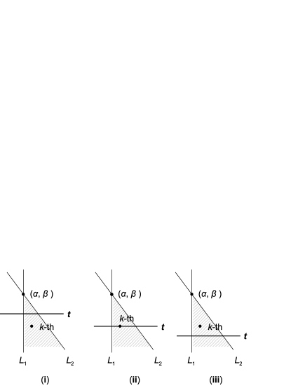
Figure 4: The three possible cases for a given value $t$.

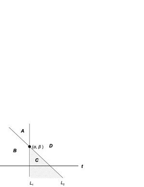
Figure 5: The four regions above (exclusive) the line $y=t.$

Now let us look at the total time complexity. Since the loop consists of at most $O(\log n)$ iterations and each iteration takes $O(n\log n)$ time, the total time complexity of the loop is $O(n\log^{2}n)$. By combining this with the time for the input transformation and sorting, we have the following theorem.

Theorem 6

: Given two $n$-point multisets $P\subseteq\mathbb{R}^{2}$ and $Q\subseteq\mathbb{R}^{2}$, a positive integer $k$, two linear constraints $L_{1}$ and $L_{2}$, and a linear objective function $f:\mathbb{R}^{2}\rightarrow\mathbb{R}$, the $k^{th}$ largest objective value among all objective values of points in $(P\oplus Q)_{L_{1},L_{2}}$ can be found in $O(n\log^{2}n)$ time.

Theorem 7

: For linear objective functions, the Minkowski Sum Selection problem with two linear constraints can be solved in expected $O(n\log n)$ time.

Proof: Due to the space limitation, we leave the proof to Appendix D.      

5 Minkowski Sum Selection with $\lambda>2$ Constraints

Let $\lambda$ be a fixed integer greater than two. In the following theorem, we summarize our results of the Minkowski Sum Selection for the case where $\lambda$ linear constraints are given and the objective function is linear. Due to the space limitation, we leave the proof to Appendix E.

Theorem 8

: Let $\lambda$ be any fixed integer larger than two. The Minkowski Sum Selection problem with $\lambda$ constraints and a linear objective function is asymptotically equivalent to the Minkowski Sum Selection problem with two linear constraints and a linear objective function.

6 Minkowski Sum Finding

In the Minkowski Sum Finding problem, given two $n$-point multisets $P,Q$, a set of $\lambda$ inequalities $Ar\geq b$, an objective function $f(x,y)$ and a real number $\delta$, we are required to find a point $v^{*}=(x^{*},y^{*})$ among all points in $(P\oplus Q)_{Ar\geq b}$ which minimizes $|f(x^{*},y^{*})-\delta|$. In this section, we show how to cope with an objective function of the form $f(x,y)=ax+by$ or $f(x,y)=\frac{by}{ax}$ based on the algorithms proposed by Bernholt et al. [5]. Instead of finding the point $v^{*}=(x^{*},y^{*})$, we would like to focus on computing the value of $|f(x^{*},y^{*})-\delta|$. The point $v^{*}=(x^{*},y^{*})$ can be easily constructed from the computed information. Before moving on to the algorithm, let us look at the lower bound of the problem.

Lemma 2

: The Minkowski Sum Finding problem with an objective function of the form $f(x,y)=ax+by$ or $f(x,y)=\frac{by}{ax}$ has a lower bound of $\Omega(n\log n)$ in the algebraic decision tree model.

Proof: Given two real number sets $A=\{a_{1},\ldots,a_{n}\}$ and $B=\{b_{1},\ldots,b_{n}\}$, the Set Disjointness problem is to determine whether or not $A\cap B=\emptyset$. It is known the Set Disjointness problem has a lower bound of $\Omega(n\log n)$ in the algebraic decision tree model [2]. We first prove that the Set Disjointness problem is linear-time reducible to the Minkowski Sum Finding problem with the objective function $f(x,y)=y$. Let $P=\{(1,a_{1}),\ldots,(1,a_{n})\}$, $Q=\{(1,-b_{1}),\ldots,(1,-b_{n})\}$, and $(x^{*},y^{*})$ be the point in $(P\oplus Q)$ such that $y^{*}$ is closest to zero. Then $(x^{*},y^{*})=(2,0)$ if and only if $A\cap B\neq\emptyset$. Similarly, we can prove that the Set Disjointness problem is linear-time reducible to the Minkowski Sum Finding problem with the objective function $f(x,y)=\frac{y}{x}$. Let $P=\{(1,a_{1}),\ldots,(1,a_{n})\}$, $Q=\{(1,-b_{1}),\ldots,(1,-b_{n})\}$, and $(x^{*},y^{*})$ be the point in $(P\oplus Q)$ such that $\frac{y^{*}}{x^{*}}$ is closest to zero. Then $(x^{*},y^{*})=(2,0)$ if and only if $A\cap B\neq\emptyset$.      

Now, let us look at how to cope with a linear objective function $f(x,y)=ax+by$. Without loss of generality, we assume $\delta=0$; otherwise we may perform some input transformations first. Thus, the goal is to compute the value of $\min\{|ax+by|:(x,y)\in(P\oplus Q)_{Ar\geq b}\}$.

Lemma 3

: Divide the $xy$-plane into two parts: $D_{1}=\{(x,y):ax+by\geq 0\}$ and $D_{2}=\{(x,y):ax+by<0\}$. Given two points $v_{1}=(x_{1},y_{1})$ and $v_{2}=(x_{2},y_{2})$ in the same part, let $v_{\gamma}=(x_{\gamma},y_{\gamma})=\gamma v_{1}+(1-\gamma)v_{2}$, where $\gamma\in[0,1]$. Then we have $|ax_{\gamma}+by_{\gamma}|\geq\min{(|ax_{1}+by_{1}|,|ax_{2}+by_{2}|)}$.

Proof: It is easy to see the lemma holds if $b=0$. Without loss of generality, let $x_{1}\geq x_{2}$ and $b\neq 0$. We only prove the case where both $v_{1}$ and $v_{2}$ are in $D_{1}$, and the other case can be proved in a similar way. Now consider the following two situations: (1) $|ax_{1}+by_{1}|\leq|ax_{2}+by_{2}|$ and (2) $|ax_{1}+by_{1}|>|ax_{2}+by_{2}|$. In the first situation, by $|ax_{1}+by_{1}|\leq|ax_{2}+by_{2}|$, $ax_{1}+by_{1}\geq 0$, and $ax_{2}+by_{2}\geq 0$, we can derive that $b(y_{2}-y_{1})\geq a(x_{1}-x_{2})$. Let $v^{\prime}=(x^{\prime},y^{\prime})$ satisfy $ax_{1}+by_{1}=ax^{\prime}+by^{\prime}$ and $x^{\prime}=x_{\gamma}=\gamma x_{1}+(1-\gamma)x_{2}$. It follows that $y^{\prime}=\frac{a}{b}(1-\gamma)(x_{1}-x_{2})+y_{1}$. By $y_{\gamma}=\gamma y_{1}+(1-\gamma)y_{2}=(1-\gamma)(y_{2}-y_{1})+y_{1}$, we have $by_{\gamma}\geq by^{\prime}$. Thus, $|ax_{\gamma}+by_{\gamma}|\geq|ax^{\prime}+by^{\prime}|=|ax_{1}+by_{1}|$. In the second situation, $b(y_{1}-y_{2})>a(x_{2}-x_{1})$. Let $v^{\prime\prime}=(x^{\prime\prime},y^{\prime\prime})$ satisfy $ax_{2}+by_{2}=ax^{\prime\prime}+by^{\prime\prime}$ and $x^{\prime\prime}=x_{\gamma}=\gamma x_{1}+(1-\gamma)x_{2}$. It follows that $y^{\prime\prime}=\frac{a}{b}\gamma(x_{2}-x_{1})+y_{2}$. By $y_{\gamma}=\gamma y_{1}+(1-\gamma)y_{2}=\gamma(y_{1}-y_{2})+y_{2}$, we have $by_{\gamma}>by^{\prime\prime}$. Thus, $|ax_{\gamma}+by_{\gamma}|>|ax^{\prime\prime}+by^{\prime\prime}|=|ax_{2}+by_{2}|$. Therefore, $|ax_{\gamma}+by_{\gamma}|\geq\min{(|ax_{1}+by_{1}|,|ax_{2}+by_{2}|)}$ if $ax_{1}+by_{1}\geq 0$ and $ax_{2}+by_{2}\geq 0$.      

Let $D_{1}=\{(x,y):ax+by\geq 0\}$ and $D_{2}=\{(x,y):ax+by<0\}$. Let $R_{1}$ be the vertices of the convex hull of $(P\oplus Q)_{Ar\geq b,ax+by\geq 0}$ and $R_{2}$ be the vertices of the convex hull of $(P\oplus Q)_{Ar\geq b,ax+by<0}$. By Theorem 3, we can compute $R_{1}$ and $R_{2}$ in $O(\lambda\log\lambda+\lambda\cdot n\log n)$ time. Let $sol_{1}=\min\{|ax+by|:(x,y)\in(P\oplus Q)_{Ar\geq b}\cap D_{1}\}$ and $sol_{2}=\min\{|ax+by|:(x,y)\in(P\oplus Q)_{Ar\geq b}\cap D_{2}\}$. By Lemma 3, we have $sol_{1}=\min\{|ax+by|:(x,y)\in R_{1}\}$ and $sol_{2}=\min\{|ax+by|:(x,y)\in R_{2}\}$. Note that both the sizes of $R_{1}$ and $R_{2}$ are bounded above by $O(\lambda\cdot n)$. Therefore, $sol_{1}$ and $sol_{2}$ are computable in $O(\lambda\cdot n)$ time by examining all points in $R_{1}$ and $R_{2}$. Finally, we have the solution is the minimum of $sol_{1}$ and $sol_{2}$. The total time complexity is $O(\lambda\log\lambda+\lambda\cdot n\log n)$, and we have the following theorem.

Theorem 9

: Let $\lambda$ be any fixed nonnegative integer. The Minkowski Sum Finding problem with $\lambda$ constraints and a linear objective function can be solved in optimal $O(n\log n)$ time.

Next, we see how to cope with an objective function of the form $f(x,y)=\frac{by}{ax}$. Without loss of generality, we assume $\delta=0$ and $a=b=1$; otherwise we may perform some input transformations first. Thus, the goal is to compute the value of $\min\{|\frac{y}{x}|:(x,y)\in(P\oplus Q)_{Ar\geq b}\}$. For technical reasons, we define $\frac{y}{x}=\infty$ if $x=0$. A function $f:D\rightarrow(\mathbb{R}\cup{\infty})$ defined on a convex subset $D$ of $\mathbb{R}^{2}$ is $quasiconcave$ if whenever $v_{1},v_{2}\in D$ and $\gamma\in[0,1]$ then $f(\gamma\cdot v_{1}+(1-\gamma)\cdot v_{2})\geq\min\{f(v_{2}),f(v_{2})\}.$

Lemma 4

: Let $D_{1}=\{(x,y)\in\mathbb{R}^{2}:x\geq 0,y\geq 0\}$, $D_{2}=\{(x,y)\in\mathbb{R}^{2}:x\leq 0,y\geq 0\}$, $D_{3}=\{(x,y)\in\mathbb{R}^{2}:x\leq 0,y\leq 0\}$, and $D_{4}=\{(x,y)\in\mathbb{R}^{2}:x\geq 0,y\leq 0\}$. Define function $f_{i}:D_{i}\rightarrow\mathbb{R}$ by letting $f_{i}(x,y)=|\frac{y}{x}|$ for each $i=1,2,3,4.$ Then we have function $f_{i}$ is quasiconcave for each $i=1,2,3,4$.

Proof: We only prove that $f_{1}$ is quasiconcave. The proofs for $f_{2}$, $f_{3}$, and $f_{4}$ can be derived in a similar way. Let $v_{1}=(x_{1},y_{1})\in D_{1}$, $v_{2}=(x_{2},y_{2})\in D_{1}$, and $x_{1}\geq x_{2}$. Without loss of generality we may assume $x_{1}>0$ and $v_{\gamma}\not\in\{v_{1},v_{2}\}.$ Consider the following two cases.

Case 1: $\frac{y_{1}}{x_{1}}\leq{\frac{y_{2}}{x_{2}}}$. Let $v^{\prime}=(x^{\prime},y^{\prime})$ be the point which satisfies $\frac{y_{1}}{x_{1}}=\frac{y^{\prime}}{x^{\prime}}$ and $x^{\prime}=x_{\gamma}=\gamma x_{1}+(1-\gamma)x_{2}$. By $x_{1}>0$, $x_{2}\geq 0$, and ${\frac{y_{1}}{x_{1}}}\leq{\frac{y_{2}}{x_{2}}}$, we have $y_{2}\geq\frac{x_{2}}{x_{1}}y_{1}$. It follows that $y^{\prime}=(\gamma x_{1}+(1-\gamma)x_{2})\frac{y_{1}}{x_{1}}=\gamma y_{1}+(1-\gamma)\frac{x_{2}}{x_{1}}y_{1}\leq\gamma y_{1}+(1-\gamma)y_{2}=y_{\gamma}$. By $0<x^{\prime}=x_{\gamma}$ and $0\leq y^{\prime}\leq y_{\gamma}$, we have $|\frac{y_{\gamma}}{x_{\gamma}}|=\frac{y_{\gamma}}{x_{\gamma}}\geq\frac{y^{\prime}}{x^{\prime}}=\frac{y_{1}}{x_{1}}=|\frac{y_{1}}{x_{1}}|\geq\min\{|{\frac{y_{1}}{x_{1}}}|,|{\frac{y_{2}}{x_{2}}}|\}$.

Case 2: ${\frac{y_{1}}{x_{1}}}>{\frac{y_{2}}{x_{2}}}$. Let $v^{\prime\prime}=(x^{\prime\prime},y^{\prime\prime})$ be the point which satisfies $\frac{y_{2}}{x_{2}}=\frac{y^{\prime\prime}}{x^{\prime\prime}}$ and $x^{\prime\prime}=x_{\gamma}=\gamma x_{1}+(1-\gamma)x_{2}$. By $x_{1}>0$ and ${\frac{y_{1}}{x_{1}}}>{\frac{y_{2}}{x_{2}}}$, we have $y_{1}>\frac{x_{1}}{x_{2}}y_{2}$. It follows that $y^{\prime\prime}=(\gamma x_{1}+(1-\gamma)x_{2})\frac{y_{2}}{x_{2}}=\gamma\frac{x_{1}}{x_{2}}y_{2}+(1-\gamma)y_{2}<\gamma y_{1}+(1-\gamma)y_{2}=y_{\gamma}$. By $0<x^{\prime\prime}=x_{\gamma}$ and $0\leq y^{\prime\prime}\leq y_{\gamma}$, we have $|\frac{y_{\gamma}}{x_{\gamma}}|=\frac{y_{\gamma}}{x_{\gamma}}>\frac{y^{\prime\prime}}{x^{\prime\prime}}=\frac{y_{2}}{x_{2}}=|{\frac{y_{2}}{x_{2}}}|\geq\min\{|{\frac{y_{1}}{x_{1}}}|,|{\frac{y_{2}}{x_{2}}}|\}$.      

Let $D_{1}=\{(x,y)\in\mathbb{R}^{2}:x\geq 0,y\geq 0\}$, $D_{2}=\{(x,y)\in\mathbb{R}^{2}:x\leq 0,y\geq 0\}$, $D_{3}=\{(x,y)\in\mathbb{R}^{2}:x\leq 0,y\leq 0\}$, and $D_{4}=\{(x,y)\in\mathbb{R}^{2}:x\geq 0,y\leq 0\}$. Let $R_{i}$ be the vertices of the convex hull of $(P\oplus Q)_{Ar\geq b}\cap D_{i}$ for $i=1,2,3,4$. By Theorem 3, each $R_{i}$ is computable in $O(\lambda\log\lambda+\lambda\cdot n\log n)$ time. Let $sol_{i}=\min\{|\frac{y}{x}|:(x,y)\in(P\oplus Q)_{Ar\geq b}\cap D_{i}\}$ for each $i=1,2,3,4$. By Lemma 4, we have $sol_{i}=\min\{|\frac{y}{x}|:(x,y)\in R_{i}\}$ for each $i$. Note that the size of each $R_{i}$ is bounded above by $O(\lambda+n)$. Therefore, each $sol_{i}$ is computable in $O(\lambda+n)$ time by examining all points in $R_{i}$. Finally, we have the solution is $\min_{i=1}^{4}sol_{i}$. The total time complexity is $O(\lambda\log\lambda+\lambda\cdot n\log n)$, and we have the following theorem.

Theorem 10

: Let $\lambda$ be any fixed nonnegative integer. The Minkowski Sum Finding problem with $\lambda$ constraints and an objective function of the form $f(x,y)=\frac{by}{ax}$ can be solved in optimal $O(n\log n)$ time.

Appendix A: Applications to the Length-constrained Sum Selection Problem

Given a sequence $S=(s_{1},s_{2},\ldots,s_{n})$ of $n$ real numbers, and two positive integers $l$, $u$ with $l<u$, define the length and sum of a segment $S[i,j]=(s_{i},\ldots,s_{j})$ to be $length(i,j)=j-i+1$ and $sum(i,j)=\sum_{h=i}^{j}s_{h}$, respectively. A segment is said to be feasible if and only if its length is in $[l,u]$. The Length-Constrained Sum Selection problem is to find the $k^{th}$ largest sum among all sums of feasible segments of $S$.

When there are no length constraints, i.e., $l=1$ and $u=n$, the Length-Constrained Sum Selection problem becomes the Sum Selection problem. Bengtsson and Chen [3] first studied the Sum Selection problem and gave an $O(n\log^{2}n)$-time algorithm for it. Recently, Lin and Lee provided an $O(n\log n)$-time algorithm [13] for the Sum Selection problem and an expected $O(n\log(u-l+1))$-time randomized algorithm [14] for the Length-Constrained Sum Selection problem. In the following, we show how to solve the Length-Constrained Sum Selection problem in worst-case $O(n\log(u-l+1))$ time.

Algorithm

We first reduce the Length-Constrained Sum Selection problem to the Minkowski Sum Selection problem as follows. Let $P=\{p_{0},p_{1},\ldots,p_{n}\}$ and $Q=\{q_{0},q_{-1},\ldots,q_{-n}\}$, where $p_{i}=(x_{i},y_{i})=(i,\sum_{t=1}^{i}s_{t})$ and $q_{-i}=(\overline{x}_{i},\overline{y}_{i})=(-i,-\sum_{t=1}^{i}s_{t})$ for all $i=0,1,\ldots,n$.

A point $(x,y)$ in $P\oplus Q$ is said to be a feasible point if and only if $l\leq x\leq u$. Each feasible segment $S[i,j]$ corresponds to a feasible point $(x,y)=p_{j}+q_{1-i}$ in $P\oplus Q$. Thus, the Length-Constrained Sum Selection problem is equivalent to finding the $k^{th}$ largest $y$-coordinate among all $y$-coordinates of feasible points in $P\oplus Q$. We next show how to do this in $O(n\log(u-l+1))$ time. For simplicity, we assume $n$ is a multiple of $u-l$.

1. Let $i_{t}=t(u-l)$ and $j_{t}=l-t(u-l)$ for $t=0,1,\ldots,\frac{n}{u-l}$.

2. For $t\leftarrow 0$ to $\frac{n}{u-l}$ do

   1. Let $P_{t}$=$\{p_{h}\in P:i_{t}-(u-l)<h\leq i_{t}\}$ and $Q_{t}=Q_{t,1}\cup Q_{t,2}$, where $Q_{t,1}=\{q_{h}\in Q:j_{t}\leq h<j_{t}+(u-l)\}$ and $Q_{t,2}=\{q_{h}\in Q:j_{t}+(u-l)\leq h<j_{t}+2(u-l)\}.$

   2. Store the $y$-coordinates of points in $(P_{t}\oplus Q_{t,1})_{x\geq l}$ as a set $N_{t,1}$ of sorted matrices such that the sum of side lengths of the sorted matrices in $N_{t,1}$ is no greater than $c\cdot((|P_{t}|+|Q_{t,1}|)\log(|P_{t}|+|Q_{t,1}|+1))$ for some constant $c$.

   3. Store the $y$-coordinates of points in $(P_{t}\oplus Q_{t,2})_{x\leq u}$ as a set $N_{t,2}$ of sorted matrices such that the sum of side lengths of the sorted matrices in $N_{t,2}$ is no greater than $c\cdot((|P_{t}|+|Q_{t,2}|)\log(|P_{t}|+|Q_{t,2}|+1))$ for some constant $c$.
      

3. Return the $k^{th}$ largest element among the elements of sorted matrices in $\bigcup_{t=0}^{\frac{n}{(u-l)}}(N_{t,1}\cup N_{t,2})$.

The following lemma ensures the correctness.

Lemma 5

: $(P\oplus Q)_{l\leq x\leq u}=\bigcup_{t=0}^{\frac{n}{(u-l)}}((P_{t}\oplus Q_{t,1})_{l\leq x}\cup(P_{t}\oplus Q_{t,1})_{x\leq u})$.

Proof: We prove that $(P\oplus Q)_{l\leq x\leq u}\stackrel{{\scriptstyle(1)}}{{=}}\bigcup_{t=0}^{\frac{n}{(u-l)}}(P_{t}\oplus Q)_{l\leq x\leq u}\stackrel{{\scriptstyle(2)}}{{=}}\bigcup_{t=0}^{\frac{n}{(u-l)}}(P_{t}\oplus Q_{t})_{l\leq x\leq u}\stackrel{{\scriptstyle(3)}}{{=}}\bigcup_{t=0}^{\frac{n}{(u-l)}}((P_{t}\oplus Q_{t,1})_{l\leq x\leq u}\cup(P_{t}\oplus Q_{t,2})_{l\leq x\leq u})\stackrel{{\scriptstyle(4)}}{{=}}\bigcup_{t=0}^{\frac{n}{(u-l)}}((P_{t}\oplus Q_{t,1})_{l\leq x}\cup(P_{t}\oplus Q_{t,2})_{x\leq u}).$ It is clear that equations (1) and (3) are true, so only equations (2) and (4) remain to be proved.

We first prove equation (2) by showing that $(P_{t}\oplus Q)_{l\leq x\leq u}=(P_{t}\oplus Q_{t})_{l\leq x\leq u}.$ Suppose for contradiction that there exist $p_{i}\in P_{t}$ and $q_{j}\not\in Q_{t}$ such that $l\leq x_{i}+\overline{x}_{j}=i+j\leq u.$ By $p_{i}\in P_{t}$, we have $(t-1)(u-l)<i\leq t(u-l)$; by $q_{j}\not\in Q_{t}$, we have either $j<l-t(u-l)$ or $j\geq l-(t-2)(u-l)$. It follows that $i+j$ is either less than $l$ or larger than $u$, a contradiction. To prove equation (4), it suffices to prove that all points in $(P_{t}\oplus Q_{t,1})$ must have $x$-coordinates less than $u$ and all points in $(P_{t}\oplus Q_{t,2})$ must have $x$-coordinates larger than $l$. Let $p_{i}\in P_{t}$, $q_{j}\in Q_{t,1}$ and $q_{j^{\prime}}\in Q_{t,2}$. It follows that $(t-1)(u-l)<x_{i}=i\leq t(u-l)$, $l-t(u-l)\leq\overline{x}_{j}=j<l-(t-1)(u-l)$, and $l-(t-1)(u-l)\leq\overline{x}_{j^{\prime}}=j^{\prime}<l-(t-2)(u-l)$. Thus, we have $x_{i}+\overline{x}_{j}=i+j<u$ and $l<x_{i}+\overline{x}_{j^{\prime}}=i+j^{\prime}$.      

Since $|P_{t}|,|Q_{t,1}|$, and $|Q_{t,2}|$ are no greater than $(u-l)$ for all $t$, each execution of Step 2.b and Step 2.c can be done in $O((u-l)\log(u-l+1))$ time by Lemma 1. There are total $\frac{n}{u-l}+1$ iterations of the for-loop in Step 2, so the total time spent on Step 2.b and Step 2.c is $O(n\log(u-l+1)).$ The sum of side lengths of sorted matrices in $\bigcup_{t=0}^{\frac{n}{(u-l)}}(N_{t,1}\cup N_{t,2})$ is $O(\sum_{t=0}^{\frac{n}{u-l}}\sum_{i=1}^{2}(|P_{t}|+|Q_{t,i}|)\log(|P_{t}|+|Q_{t,i}|+1))=O(\sum_{t=0}^{\frac{n}{u-l}}(u-l)\log(u-l+1))=O(n\log(u-l+1))$. Therefore, by Theorem 1, Step 3 can be done in $O(n\log(u-l+1))$ time. Putting everything together, we have that the total running time is $O(n\log(u-l+1))$.

Theorem 11

: The Length-Constrained Sum Selection problem can be solved in $O(n\log(u-l+1))$ time.

Appendix B: Applications to the Density Finding Problem

Given a sequence of number pairs $S=((s_{1},w_{1}),(s_{2},w_{2}),\ldots,(s_{n},w_{n}))$ where $w_{i}>0$ for $i=1,2,\ldots,n$, two positive numbers $l,u$ with $l<u$, and a real number $\delta$, let segment $S(i,j)$ of $S$ be the consecutive subsequence of $S$ between indices $i$ and $j$. Define the sum $s(i,j)$, width $w(i,j)$, and density $d(i,j)$ of segment $S(i,j)$ to be $\sum_{r=i}^{j}s_{r}$, $\sum_{r=i}^{j}w_{r}$ and $\frac{s(i,j)}{w(i,j)},$ respectively. A segment $S(i,j)$ is said to be feasible if and only if $l\leq w(i,j)\leq u$. The Density Finding problem is to compute the density of the feasible segment $S(i^{*},j^{*})$ which minimizes $|d(i^{*},j^{*})-\delta|$. Lee $et~{}al.$ [12] proved that the Density Finding problem has a lower bound of $\Omega(n\log n)$ in the algebraic decision tree model and provided an $O(n\log^{2}m)$ algorithm for it, where $m=\min(\lfloor\frac{u-l}{w_{min}}\rfloor,n)$ and $w_{min}=\min_{1\leq r\leq n}w_{r}$. In the following we describe how to solve the Density Finding problem in $O(n\log n)$ time by using the algorithm developed in Section 6.

Let $w(1,0)=0$ and $s(1,0)=0$. Compute in $O(n)$ time the following two point sets: $P=\{(w(1,i),s(1,i))|0\leq i\leq n\}$ and $Q=\{(-w(1,i),-s(1,i))|0\leq i\leq n)\}$. Note that each feasible segment $S(i,j)$ of $S$ corresponds to a point $(w(1,j)-w(1,i-1),s(1,j)-s(1,i-1))$ in $(P\oplus Q)_{l\leq x\leq u}$. Thus, the problem is reduced to finding the point $(x^{*},y^{*})$ in $(P\oplus Q)_{l\leq x\leq u}$ such that $|\frac{y^{*}}{x^{*}}-\delta|$ is minimized. By Theorem 10, it can be done in $O(n\log n)$ time, so we have the following theorem.

Theorem 12

: The Density Finding problem can be solved in optimal $O(n\log n)$ time.

Appendix C: Minkowski Sum Selection with Two Parallel Constraints

Now we explain how to solve the Minkowski Sum Selection problem with two parallel constraints in $O(n\log n)$ time. Given $P=\{(x_{1,1},y_{1,1}),\ldots,(x_{1,n},y_{1,n})\}$, $Q=\{(x_{2,1},y_{2,1}),\ldots,(x_{2,n},y_{2,n})\}$, a positive integer $k$, two parallel constraints $L_{1}$: $ax+by\geq c_{1}$ and $L_{2}$: $ax+by\leq c_{2}$ with $c_{1}\leq c_{2}$, and a linear objective function $f(x,y)=dx+ey$, where $a$, $b$, $c_{1}$, $c_{2}$, $d$, and $e$ are all constants, we want to find the $k^{th}$ largest objective value among all objective values of points in $(P\oplus Q)_{L_{1},L_{2}}$. Note that if the constraints $L_{1}$ and $L_{2}$ are of the forms $ax+by\leq c_{1}$ and $ax+by\leq c_{2}$ respectively, this problem degenerates to the Minkowski Sum Selection problem with one constraint and can be solved by the algorithm stated in Section 3. We perform the following transformation.

1. Change the content of $P$ and $Q$ to $\{(ax_{1,1}+by_{1,1},dx_{1,1}+ey_{1,1}),\ldots,(ax_{1,n}+by_{1,n},dx_{1,n}+ey_{1,n})\}$, and $\{(ax_{2,1}+by_{2,1},dx_{2,1}+ey_{2,1}),\ldots,(ax_{2,n}+by_{2,n},dx_{2,n}+ey_{2,n})\}$, respectively.

2. Change the constraints from $ax+by\geq c_{1}$ and $ax+by\leq c_{2}$ to $x\geq c_{1}$ and $x\leq c_{2}$, respectively.

3. Change the objective function from $dx+ey$ to $y$.

This transformation can be done in $O(n)$ time and the answer remains the same. Hence from now on, our goal becomes to find the $k^{th}$ largest $y$-coordinate on the constrained Minkowski sum of $P$ and $Q$ subject to the constraints $L_{1}$: $x\geq c_{1}$ and $L_{2}$: $x\leq c_{2}$. First we sort $P$ and $Q$ into $P_{x}$ and $Q_{x}$ in nondecreasing order of $x$-coordinates, respectively in $O(n\log n)$ time. Let $P_{x}=\{(x_{1},y_{1}),\ldots,(x_{n},y_{n})\}$ and $Q_{x}=\{(\bar{x}_{1},\bar{y}_{1}),\ldots,(\bar{x}_{n},\bar{y}_{n})\}$. For all points in $P_{x}$, we can form a partition of them according to the values of their $x$-coordinates. Let the partition be $P_{t_{1}},P_{t_{2}},\ldots,P_{t_{m}}$ where $P_{t_{i}}=\{(x_{j},y_{j})\in P_{x}:(t_{i}-1)(c_{2}-c_{1})<x_{j}\leq t_{i}(c_{2}-c_{1})\}$, and $t_{i}$ be an integer for $i=1,2,\ldots,m$ with $t_{1}<t_{2}<\ldots<t_{m}$. Similarly, we can partition the points in $Q_{x}$ according to the values of their $x$-coordinates. Let the partition be $Q_{\bar{t}_{1}},Q_{\bar{t}_{2}},\ldots,Q_{\bar{t}_{m^{\prime}}}$ where $Q_{\bar{t}_{i}}=\{(\bar{x}_{j},\bar{y}_{j})\in Q_{x}:c_{1}-\bar{t}_{i}(c_{2}-c_{1})\leq\bar{x}_{j}<c_{1}-(\bar{t}_{i}-1)(c_{2}-c_{1})\}$, and $\bar{t}_{i}$ be an integer for $i=1,2,\ldots,m^{\prime}$ with $\bar{t}_{1}<\bar{t}_{2}<\ldots<\bar{t}_{m^{\prime}}$. Since $P_{x}$ and $Q_{x}$ are sorted in nondecreasing order of $x$-coordinates respectively, the two partitions can be easily produced in linear time. In the following, we show the algorithm for this problem.

1. Let $P_{t_{1}},P_{t_{2}},\ldots,P_{t_{m}}$ and $Q_{\bar{t}_{1}},Q_{\bar{t}_{2}},\ldots,Q_{\bar{t}_{m^{\prime}}}$ be defined as the above.

2. For $i\leftarrow 1$ to $m$ do

   1. To find $Q_{t_{i}}=\{(\bar{x}_{j},\bar{y}_{j})\in Q_{x}:c_{1}-t_{i}(c_{2}-c_{1})\leq\bar{x}_{j}<c_{1}-(t_{i}-1)(c_{2}-c_{1})\}$ and $Q_{t_{i}-1}=\{(\bar{x}_{j},\bar{y}_{j})\in Q_{x}:c_{1}-(t_{i}-1)(c_{2}-c_{1})\leq\bar{x}_{j}<c_{1}-(t_{i}-2)(c_{2}-c_{1})\}.$

   2. If $Q_{t_{i}}$ exists, store the $y$-coordinates of points in $(P_{t_{i}}\oplus Q_{t_{i}})_{x\geq c_{1}}$ as a set $N_{i,1}$ of sorted matrices such that the sum of side lengths of the sorted matrices in $N_{i,1}$ is no greater than $c\cdot((|P_{t_{i}}|+|Q_{t_{i}}|)\log(|P_{t_{i}}|+|Q_{t_{i}}|+1))$ for some constant $c$.

   3. If $Q_{t_{i}-1}$ exists, store the $y$-coordinates of points in $(P_{t_{i}}\oplus Q_{t_{i}-1})_{x\leq c_{2}}$ as a set $N_{i,2}$ of sorted matrices such that the sum of side lengths of the sorted matrices in $N_{i,2}$ is no greater than $c\cdot((|P_{t_{i}}|+|Q_{t_{i}-1}|)\log(|P_{t_{i}}|+|Q_{t_{i}-1}|+1))$ for some constant $c$.
      

3. Return the $k^{th}$ largest element among the elements of sorted matrices in $\bigcup_{i=1}^{m}(N_{i,1}\cup N_{i,2})$.

By the proof of Lemma 5, we ensure the correctness of the algorithm. Now we consider the time complexity of the algorithm. By Lemma 1, each execution of Step 2.b and Step 2.c can be done in $O((|P_{t_{i}}|+|Q_{t_{i}}|)\log(|P_{t_{i}}|+|Q_{t_{i}}|+1))$ and $O((|P_{t_{i}}|+|Q_{t_{i}-1}|)\log(|P_{t_{i}}|+|Q_{t_{i}-1}|+1))$ time, respectively. Since there are total $m$ iterations of the for-loop in Step 2, it follows that

$$\sum_{i=1}^{m}\big{(}(|P_{t_{i}}|+|Q_{t_{i}}|)\log(|P_{t_{i}}|+|Q_{t_{i}}|+1)+(|P_{t_{i}}|+|Q_{t_{i}-1}|)\log(|P_{t_{i}}|+|Q_{t_{i}-1}|+1)\big{)}$$

$$\leq \sum_{i=1}^{m}\big{(}(|P_{t_{i}}|+|Q_{t_{i}}|)\log(2n+1)+(|P_{t_{i}}|+|Q_{t_{i}-1}|)\log(2n+1)\big{)}$$

$$\leq \sum_{i=1}^{m}(2|P_{t_{i}}|+|Q_{t_{i}}|+|Q_{t_{i}-1}|)\log(2n+1)\leq(4n)\log(2n+1).$$

Therefore, the total time spent on Step 2 is $O(n\log n)$ and the sum of the side lengths of sorted matrices in $\bigcup_{i=1}^{m}(N_{i,1}\cup N_{i,2})$ is also $O(n\log n)$. By Theorem 1, Step 3 can be done in $O(n\log n)$ time. Putting everything together, we have that the total running time is $O(n\log n)$. The next theorem summarizes the time complexity of the algorithm.

Theorem 13

: For linear objective functions, the Minkowski Sum Selection problem with two parallel constraints can be solved in $O(n\log n)$ time.

Appendix D: A Randomized Algorithm for Minkowski Sum Selection with Two Constraints

In this section, we introduce a randomized algorithm for the Minkowski Sum Selection problem with two constraints that runs in expected $O(n\log n)$ time.

Subroutines for Minkowski Sum Selection Problem with Two Constraints

Our randomized algorithm is based on three subroutines for three subproblems. In this subsection, we define these subproblems and give these subroutines for them.

Before we discuss these subroutines, we introduce the notion of an order-statistic tree. An order-statistic tree is a balanced search tree with additional information, $size[z]$, stored in each node $z$ of the tree. The additional information $size[z]$ contains the total number of nodes in the subtree rooted at $z$. Define $left[z]$ and $right[z]$ are the left and right children of the node $z$, respectively. The additional information $size[z]$ equals to $size[left[z]]+size[right[z]]+1$ if $z$ is an internal node, and one if $z$ is a leaf node. Let $key[z]$ be the key of the node $z$. The rank of a given value $x$ can be determined in $O(\log n)$ time by using the order-statistic tree $T$, where $n$ is the number of nodes in $T$. That is, we can find the rank $r(x,T)=|\{y|y\in T,key[y]>x\}|$ in $O(\log n)$ time, retrieve an element in $T$ with a given rank in $O(\log n)$ time and maintain both insertion and deletion operations in $T$ in $O(\log n)$ time.

The first subproblem is the reporting version of the Minkowski Sum Range Query problem with two constraints, which is defined as follows: Given two $n$-point multisets $P$, $Q$, two constraints $L_{1}$, $L_{2}$, and two real numbers $s_{l}$, $s_{r}$ with $s_{l}\leq s_{r}$, we want to output all points in $(P\oplus Q)_{L_{1},L_{2}}$, such that their $y$-coordinates are in the range $[s_{l},s_{r}]$. Before we discuss this subproblem, we consider a weak version of this subproblem. The weak version is defined as above, except that we assign the constraints $L_{1}$: $ax+by\geq c_{1}$ and $L_{2}$: $ax+by\leq c_{2}$, where $c_{1}\leq c_{2}$. To solve the weak version, we perform the input transformation stated in Section 4.1.1 to change $L_{1}$ and $L_{2}$ to $x\geq c_{1}$ and $x\leq c_{2}$ respectively. Then we sort $P$ and $Q$ into $P_{x}$ and $Q_{x}$ respectively in nondecreasing order of $x$-coordinates. Let $P_{x}=((x_{1},y_{1}),\ldots,(x_{n},y_{n}))$ and $Q_{x}=((\bar{x}_{1},\bar{y}_{1}),\ldots,(\bar{x}_{n},\bar{y}_{n}))$. Denote by $l_{i}$ the smallest index in $Q_{x}$ such that $x_{i}+\bar{x}_{l_{i}}\geq c_{1}$ and by $r_{i}$ the largest index in $Q_{x}$ such that $x_{i}+\bar{x}_{r_{i}}\leq c_{2}$. It is guaranteed that $l_{i}\geq l_{j}$ and $r_{i}\geq r_{j}$ for any $i<j$. For this reason, it can be easily done to find all $l_{i}$ and $r_{i}$ for $i=1,\ldots,n$ in total $O(n)$ time. We use the points in $Q_{x}$ to construct an order-statistic tree with the values of $y$-coordinates as keys. For the index $j$, we use the points $(\bar{x}_{i},\bar{y}_{i})$ in $Q_{x}$ for $i=l_{j},\ldots,r_{j}$ to construct an order-statistic tree $T(j)$ in $O((r_{j}-l_{j})\log(r_{j}-l_{j}))$ time. Because $T(j)$ is also a balanced binary search tree, we can report all points in $T(j)$ whose $y$-coordinates are in $[s_{l}-y_{j},s_{r}-y_{j}]$ by binary search in $O(log(r_{j}-l_{j})+h_{j})$ time, where $h_{j}$ is the total number of points whose $y$-coordinates are in $[s_{l}-y_{j},s_{r}-y_{j}]$. At each iteration $j$, we can maintain $T(j+1)$ dynamically by deleting all points $(\bar{x}_{i},\bar{y}_{i})$ in $T(j)$ for $i=r_{j+1}+1,\ldots,r_{j}$ and inserting all points $(\bar{x}_{i^{\prime}},\bar{y}_{i^{\prime}})$ into $T(j)$ for $i^{\prime}=l_{j+1},\ldots,l_{j}-1$. It suffices to iterate on each index $j$ to find all points in $(P\oplus Q)_{L_{1},L_{2},y\leq s_{r},y\geq s_{l}}$. Hence, we can solve the weak version in $O(n\log n+h)$ time, where $h$ is the output size.

Now we show how to solve the reporting version of the Minkowski Sum Range Query problem with two constraints by the weak version stated above. By performing the transformation stated in Section 4.1.1, $L_{1}$ and $L_{2}$ are changed to $x\geq c_{1}$ and $ax+by\geq c_{2}$ respectively. We divide the feasible region bounded by $L_{1}$, $L_{2}$, and $s_{l}\leq y\leq s_{r}$ into several subregions. For each subregion, it can be solved by the subroutine for the weak version of this subproblem. Let $L_{1}^{\prime}$ be the line that is parallel to $L_{1}$ and passes through the intersection point of $L_{2}$ and $y=s_{r}$, and $L_{2}^{\prime}$ be the line that is parallel to $L_{2}$ and passes through the intersection point of $L_{1}$ and $y=s_{r}$. By the location of the intersection point of $L_{1}^{\prime}$ and $L_{2}^{\prime}$, we have four possible cases: (a) the intersection point lies in the line $y=s_{l}$; (b) the intersection point lies below the line $y=s_{l}$; (c) the intersection point lies above the line $y=s_{r}$; (d) the intersection point lies between $y=s_{l}$ and $y=s_{r}$. See Figure 6 for an illustration. We solve the reporting version according to the four possible cases respectively. For Case (a), we consider the parallelogram formed by $L_{2}$, $L_{2}^{\prime}$, $y\leq s_{r}$, and $y\geq s_{l}$ and all feasible points in this parallelogram can be reported by the subroutine of the weak version. Next we consider the rectangle formed by $L_{1}$, $L_{1}^{\prime}$, $y\leq s_{r}$, and $y\geq s_{l}$ and all feasible points in this rectangle can be reported in the same way, except we have to remove the redundant points in the area formed by $L_{1}^{\prime}$, $L_{2}^{\prime}$, and $y\leq s_{r}$. When we report each feasible point in the rectangle formed by $L_{1}$, $L_{1}^{\prime}$, $y\leq s_{r}$, and $y\geq s_{l}$, we can check whether this point lies in the area formed by $L_{1}^{\prime}$, $L_{2}^{\prime}$, and $y\leq s_{r}$ in $O(1)$ time. If this point lies in this area, we discard this point, or we report it. For Case (b), we can also solve this case in the same way of Case (a), except the redundant points are in the area formed by $L_{1}^{\prime}$, $L_{2}^{\prime}$, $y\leq s_{r}$, and $y\geq s_{l}$. For each redundant point, however, the removal can be also easily done in $O(1)$ time.

For Case (c), we must divide the triangle formed by $L_{1}$, $L_{2}$, and $y\geq s_{l}$ in another way. Let $a$ be the intersection point of $L_{1}$ and $L_{2}$, $c$ be the intersection point of $L_{1}$ and $y\geq s_{l}$, and $b$ be the middle point of the line segment $\overline{ac}$. We can draw the line $L_{3}$ that is parallel to $y=s_{l}$ and passes through $b$, and let $d$ be the intersection point of $L_{3}$ and $L_{2}$. Let $L_{2}^{\prime\prime}$ be the line that is parallel to $L_{2}$ and passes through $b$, and $L_{1}^{\prime\prime}$ be the line that is parallel to $L_{1}$ and passes through $d$. Because the triangle formed by $L_{1}$, $L_{2}$, and $y\geq s_{l}$ is a right-angled triangle, the intersection point of $L_{1}^{\prime\prime}$ and $L_{2}^{\prime\prime}$ must lie in the line $y=s_{l}$. We first report the feasible points in the parallelogram formed by $L_{1}$, $L_{1}^{\prime\prime}$, $L_{2}$, and $L_{2}^{\prime\prime}$ by the subroutine of the weak version. Then we report the feasible points in the parallelogram formed by $L_{3}$, $y\geq s_{l}$, $L_{2}$, and $L_{2}^{\prime\prime}$ in the same way and remove the redundant points, i.e., the points lie in the area formed by $L_{3}$, $L_{1}^{\prime\prime}$, and $L_{2}^{\prime\prime}$. Finally, we report the feasible points in the rectangle formed by $L_{1}$, $L_{1}^{\prime\prime}$, $L_{3}$, and $y\geq s_{l}$ and remove the redundant points in the area formed by $L_{3}$, $L_{1}^{\prime\prime}$, and $L_{2}^{\prime\prime}$.

For Case (d), we report all feasible points in the parallelogram formed by $L_{2}$, $L_{2}^{\prime}$, $y\leq s_{r}$, and $y\geq s_{l}$ and in the rectangle formed by $L_{1}$, $L_{1}^{\prime}$, $y\leq s_{r}$, and $y\geq s_{l}$ with the removal of the redundant points in the area formed by $L_{1}^{\prime}$, $L_{2}^{\prime}$, and $y\leq s_{r}$. The remaining is the triangle formed by $L_{1}^{\prime}$, $L_{2}^{\prime}$, and $y\geq s_{l}$ and is just Case (c). Therefore, we can solve this triangle in the same way of Case (c). In the following, we conclude the time complexity of this problem.

Figure 6: The illustration of how to solve the reporting version.

Lemma 6

: The reporting version of the Minkowski Sum Range Query problem with two constraints can be solved in $O(n\log n+h)$ time, where $h$ is the output size.

The second subproblem, called the counting version of the Minkowski Sum Range Query problem with two constraints, is defined as before, but we only want to find the number of points in $(P\oplus Q)_{L_{1},L_{2}}$ satisfying the range query, i.e., their $y$-coordinates are between $s_{l}$ and $s_{r}$. To solve this subproblem, we make use of the procedure Ranking₂ shown in Figure 7. Let $R_{l}$ be the number of points in $(P\oplus Q)_{L_{1},L_{2}}$ that their $y$-coordinates are larger than $s_{l}$. It is obvious to see that $R_{l}$ is equal to Ranking${}_{2}(P,Q,L_{1},L_{2},f(x,y)=y,s_{l})$. Let $R_{r}$ be the number of points in $(P\oplus Q)_{L_{1},L_{2}}$ that their $y$-coordinates are larger than $s_{r}$, and $R_{r}$ is equal to Ranking${}_{2}(P,Q,L_{1},L_{2},f(x,y)=y,s_{r})$. As a result, the number of points in $(P\oplus Q)_{L_{1},L_{2},y\leq s_{r},y\geq s_{l}}$ is $R_{l}-R_{r}$ plus the number of points in $(P\oplus Q)_{L_{1},L_{2},y=s_{l}}$. Let $R$ be the number of points in $(P\oplus Q)_{L_{1},L_{2},y=s_{l}}$. $R$ can be obtained by computing Ranking${}_{1}(P,Q,y=s_{l},f(x,y)=x,c_{1})$ minus Ranking${}_{1}(P,Q,y=s_{l},f(x,y)=x,c_{2})$. Hence, we obtain the number of points in $(P\oplus Q)_{L_{1},L_{2},y\leq s_{r},y\geq s_{l}}$.

Lemma 7

: The counting version of the Minkowski Sum Range Query problem with two constraints can be solved in $O(n\log n)$ time.

The last subproblem, called the Random Sampling Minkowski Sum problem with two constraints, is defined as follows: Give two $n$-point multisets $P$, $Q$, two constraints $L_{1}$: $x\geq c_{1}$, $L_{2}$: $ax+by\geq c_{2}$, and two real numbers $s_{l}$, $s_{r}$ with $s_{l}\leq s_{r}$, we want to randomly generate $n$ points from $(P\oplus Q)_{L_{1},L_{2},y\leq s_{r},y\geq s_{l}}$ with replacement. For the ease of similar discussions, in the following we only focus on Case (a) illustrated in Figure 6 and the other cases can be solved in a similar way.

Let $N$ be the number of points in $(P\oplus Q)_{L_{1},L_{2},y\leq s_{r},y\geq s_{l}}$, $N_{1}$ be the number of points in the parallelogram $A$ formed by $L_{2}$, $L_{2}^{\prime}$, $y\leq s_{r}$ and $y\geq s_{l}$, $N_{2}$ be the number of points in the rectangle $B$ formed by $L_{1}$, $L_{1}^{\prime}$, $y\leq s_{r}$ and $y\geq s_{l}$, and $N_{3}$ be the number of points in the triangle $C$ formed by $L_{1}^{\prime}$, $L_{2}^{\prime}$ and $y\leq s_{r}$. $N$, $N_{1}$, $N_{2}$, and $N_{3}$ can be computed by the subroutine for the counting version of the Minkowski Sum Range Query problem with two constraints. For the parallelogram $A$, we can use the subroutine for the weak version of the reporting subproblem to construct the order-statistic tree $T(j)$ on points in $Q_{x}$ for $j=1,\ldots,n$. Let the size of $T(j)$ be $t_{j}$ and then $N_{1}=t_{1}+t_{2}+\ldots+t_{n}$. We first pick $n$ random integers $\bar{R}=\{\bar{r}_{1},\bar{r}_{2},\ldots,\bar{r}_{n}\}$ uniformly distributed in the range from $1$ to $N$ with replacement. Since $N=O(n^{2})$, we can sort them by radix sort and rename them such that $\bar{r}_{1}\leq\bar{r}_{2}\leq\ldots\leq\bar{r}_{n}$ in $O(n)$ time. Let $\tau_{j}=t_{1}+t_{2}+\ldots+t_{j}$. For each $j$, there exist $\bar{r}_{c},\bar{r}_{c+1},\ldots,\bar{r}_{c+d}\in\bar{R}$ such that $\tau_{j-1}<\bar{r}_{c}\leq\bar{r}_{c+1}\leq\ldots\leq\bar{r}_{c+d}\leq\tau_{j}$. For $\bar{r}_{i}\leq N_{1}$, we shall find points $\bar{s}_{c},\bar{s}_{c+1},\ldots,\bar{s}_{c+d}$ in $(P\oplus Q)_{L_{1},L_{2},y\leq s_{r},y\geq s_{l}}$ with a one-to-one correspondence to $\bar{r}_{c},\bar{r}_{c+1},\ldots,\bar{r}_{c+d}$. For each index $j$, we make a query to the order-statistic tree $T(j)$ in order to count the total number $\alpha_{j}$ of points such that their $y$-coordinates are less than $s_{l}$, i.e., $\alpha_{j}=|\{y|y\in T(j),key[y]<s_{l}\}|$. We then retrieve the point $\bar{s}_{c+i}=(\bar{x}_{q_{i}},\bar{y}_{q_{i}})$ from $T(j)$ such that $\bar{y}_{q_{i}}$ has a rank equal to $\alpha_{j}+\bar{r}_{c+i}-\tau_{j-1}$ in $T(j)$ for each $i=0,1,\ldots,d$. For $\bar{r}_{i}>N_{1}$, we record the total number of $\bar{r}_{i}$ larger than $N_{1}$, say $\phi$. We thus obtain a set of points, $\bar{S}=\{\bar{s}_{1},\ldots,\bar{s}_{N_{1}}\}$. Next we remove the points in $\bar{S}$ lying in the triangle $C$, and record the number of points removed, say $\psi$. Then we select $\phi+\psi$ points randomly from the rectangle $B$ using the same way. Combining these $\phi+\psi$ points with $\bar{S}$, we obtain the set of random sampling points.

Now we show that the sampling resulted from our random sampling subroutine is uniformly random. Let $\bar{X}=\{X_{1},X_{2},\ldots,X_{n}\}$ be any fixed random sample generated from our random sampling subroutine and $X_{i_{1}},X_{i_{2}},\ldots X_{i_{k}}$ be the points in the triangle formed by $L_{1}^{\prime}$, $L_{2}$, and $y\geq s_{l}$. The probability that this random sample occurs is exactly $(\frac{1}{N})^{k}(\frac{N_{2}}{N})^{n-k}(\frac{1}{N_{2}})^{n-k}=(\frac{1}{N})^{n}$. Thus we obtain that for any fixed random sample, the probability of occurring is the same $(\frac{1}{N})^{n}$, i.e., the random sample generated from our random sampling subroutine is uniformly random. The following lemma concludes the time complexity.

Lemma 8

: The Random Sampling Minkowski Sum problem with two constraints can be solved in expected $O(n\log n)$ time.

Algorithm

First of all, we perform the input transformation stated in Section 4.1.1. Hence we assume that the two constraints are $L_{1}$: $x\geq c_{1}$, $L_{2}$: $ax+by\geq c_{2}$ and the objective function is $f(x,y)=y$. We say a range $[s_{l},s_{r}]$ contains a point $s\in P\oplus Q$ if $s$ satisfies two linear constraints $y\geq s_{l}$ and $y\leq s_{r}$.

Let the $y$-coordinates of the points in $P\oplus Q$ be in the range $[s_{l},s_{r}]$, and $s^{*}=(x^{*},y^{*})$ be the solution of the Minkowski Sum Selection problem with two constraints. Our randomized algorithm for this problem will contract the range $[s_{l},s_{r}]$ into a smaller range $[s_{l^{\prime}},s_{r^{\prime}}]$ such that $[s_{l^{\prime}},s_{r^{\prime}}]$ contains $s^{*}$. A point $s$ is said to be feasible if $s\in(P\oplus Q)_{L_{1},L_{2}}$. Let $N$ be the number of points in $(P\oplus Q)_{L_{1},L_{2}}$. The subrange $[s_{l^{\prime}},s_{r^{\prime}}]$ will contain at most $O(N/\sqrt{n})$ feasible points. We shall repeat the contraction several times until the subrange contains at most $O(n)$ feasible points and also the solution $s^{*}$. Then we output all feasible points in this subrange by the subroutine for the reporting version of the Minkowski Sum Range Query problem with two constraints and find the solution $s^{*}$ with an appropriate rank.

We first randomly select $n$ independent feasible points $\bar{S}=\{\bar{s}_{1},\bar{s}_{2},\ldots,\bar{s}_{n}\}$ which are contained in the range $[s_{l},s_{r}]$ from $N$ feasible points by the subroutine for the Random Sampling Minkowski Sum problem in $O(n\log n)$ time. When we randomly select a feasible point in $[s_{l},s_{r}]$, the probability is $\frac{k}{N}$ that its $y$-coordinate is smaller than that of $s^{*}$. Consider this event as a Bernoulli trial with the success probability $p=\frac{k}{N}$. It is obvious to see that the total number of successes is a random variable which has a binomial distribution. Hence the expected value of the total number of successes is $\mu=np=n\frac{k}{N}$. As a result, we know the good approximation for the point of the $k^{th}$ largest $y$-coordinate among all feasible points is the point of the $e^{th}$ largest $y$-coordinate among $\bar{S}$, where $e=\lfloor np\rfloor=\lfloor n\frac{k}{N}\rfloor$.

Let $l^{\prime}=\max\{1,\lfloor n\frac{k}{N}-t\frac{\sqrt{n}}{2}\rfloor\}$ and $r^{\prime}=\min\{n,\lfloor n\frac{k}{N}+t\frac{\sqrt{n}}{2}\rfloor\}$, where $t$ is a constant and will be determined later. After the random sampling, we can find the $l^{\prime}$-th and the $r^{\prime}$-th largest $y$-coordinates in $\bar{S}$, say $s_{l^{\prime}}$ and $s_{r^{\prime}}$ respectively, by any standard selection algorithm in $O(n)$ time to obtain the subrange $[s_{l^{\prime}},s_{r^{\prime}}]$. Next, we check the following two conditions by the subroutine for the counting version of the Minkowski Sum Range Query problem with two constraints in $O(n\log n)$ time:

(1) The subrange $[s_{l^{\prime}},s_{r^{\prime}}]$ contains the solution $s^{*}$.

(2) The subrange $[s_{l^{\prime}},s_{r^{\prime}}]$ contains at most $t^{2}N/(t-1)\sqrt{n}$ $(<2tN/\sqrt{n})$ feasible points.

Let $k_{1}$ and $k_{2}$ be the total number of feasible points contained in $[s_{l},s_{l^{\prime}})$ and $[s_{l},s_{r^{\prime}}]$ respectively. If $s^{*}$ is contained in the subrange $[s_{l^{\prime}},s_{r^{\prime}}]$, we know that $k_{1}<k$ and $k_{2}\geq k$. If both of the two conditions hold, we replace the range $[s_{l},s_{r}]$ and the rank $k$ with the subrange $[s_{l^{\prime}},s_{r^{\prime}}]$ and the rank $k^{\prime}=k-k_{1}$. If any of the two conditions is violated, we repeat the above step until both of the two conditions are satisfied, i.e. we need to select $n$ random feasible points with replacement in the range $[s_{l},s_{r}]$ by running the subroutine for the Random Sampling Minkowski Sum problem again to obtain a new subrange $[s_{l^{\prime}},s_{r^{\prime}}]$ and then check the above two conditions for this new subrange.

Since this randomized algorithm for the Minkowski Sum Selection problem with two constraints starts with $N$ feasible points, after the first successful contraction, we have a new range $[s_{l^{\prime}},s_{r^{\prime}}]$ contains $O(N/\sqrt{n})$ feasible points and $s^{*}$, the point of the $k^{\prime}$-th largest $y$-coordinate among all feasible points. After the second successful contraction, we have an another subrange $[s_{l^{\prime\prime}},s_{r^{\prime\prime}}]$ which contains $O(\frac{N/\sqrt{n}}{\sqrt{n}})=O(n)$ feasible points and $s^{*}$, the point of the $k^{\prime\prime}$-th largest $y$-coordinate among all feasible points. Since the number of feasible points contained in the range $[s_{l^{\prime\prime}},s_{r^{\prime\prime}}]$ is $O(n)$, we can enumerate all feasible points in this range in $O(n\log n)$ time via the subroutine for the reporting version of the Minkowski Sum Range Query problem with two constraints and select the point of the $k^{\prime\prime}$-th largest $y$-coordinate from these feasible points by using any standard selection algorithm in $O(n)$ time.

Now we show that with high probability, the point of the $k^{th}$ largest $y$-coordinate among all feasible points contained in subrange $[s_{l^{\prime}},s_{r^{\prime}}]$ and the subrange $[s_{l^{\prime}},s_{r^{\prime}}]$ contains at most $t^{2}N/(t-1)\sqrt{n}$ feasible points. Applying the results of Matou$\check{\mbox{s}}$ek et al. [19], we have the following lemma:

Lemma 9

: Given a set of feasible points $\Theta=\{\theta_{1},\theta_{2},\ldots,\theta_{N}\}$, an index $k$ $(1\leq k\leq N)$, and an integer $n>0$, we can compute in $O(n\log n)$ time an interval $[s_{l^{\prime}},s_{r^{\prime}}]$, such that, with probability $1-1/\Omega(\sqrt{n})$, the point of the $k^{th}$ largest $y$-coordinate among $\Theta$ lies within this interval, and the number of points in $\Theta$ that lie within the interval is at most $N/\Omega(\sqrt{n})$.

By the results given by Matou$\check{\mbox{s}}$ek et al. [19], we can choose $t=3$. Therefore, we just need to repeat the contraction step at most twice on average in the randomized algorithm for the Minkowski Sum Selection problem with two constraints. We conclude the time complexity of the randomized algorithm in the following theorem.

Theorem 14

: For linear objective functions, the Minkowski Sum Selection problem with two linear constraints can be solved in expected $O(n\log n)$ time.

7 Appendix E: Minkowski Sum Selection with $\lambda>2$ Constraints

In the following, we describe how to solve the Minkowski Sum Selection problem with $\lambda>2$ constraints and a linear objective function by using Algorithm Selection₂ and Algorithm Ranking₂. The pseudocodes of Algorithm Selection₂ and Algorithm Ranking₂ are given in Figure 7 and Figure 8, respectively. The running time of Algorithm Selection₂ is $O(n\log^{2}n)$ by Theorem 6, and the running time of Algorithm Ranking₂ is $O(n\log n)$.

Algorithm Selection${}_{2}(P,Q,L_{1},L_{2},f,k)$
Input: $P\subseteq\mathbb{R}^{2}$ and $Q\subseteq\mathbb{R}^{2}$ are two multisets; $L_{1}$ and $L_{2}$ are linear
	constraints; $f:{\mathbb{R}^{2}}\rightarrow\mathbb{R}$ is a linear objective function; $k$ is a positive integer.
Output: The $k^{th}$ largest value among all objective values of points in $(P\oplus Q)_{L_{1},L_{2}}$.
1	Perform the input transformation in Section 4.1. Let $L_{1}:x\geq c_{1}$ and
	$L_{2}:ax+by\geq c_{2}$ be the resulting constraints after the input transformation.
	/*Assume that $a<0$ and $b<0$.*/
2	Sort $P$ and $Q$ into $P_{y}$ and $Q_{y}$, respectively, in nondecreasing order of $y$-coordinates.
3	Let $P_{y}=((x^{\prime}_{1},y^{\prime}_{1}),\ldots,(x^{\prime}_{n},y^{\prime}_{n}))$ and $Q_{y}=((\bar{x}^{\prime}_{1},\bar{y}^{\prime}_{1}),\ldots,(\bar{x}^{\prime}_{n},\bar{y}^{\prime}_{n}))$.
4	Denote by $Y$ the sorted matrix of dimensions $n\times n$ where the $(i,j)$-th element
	is $y^{\prime}_{i}+\bar{y}^{\prime}_{j}$.
5	$u\leftarrow n^{2}$; $l\leftarrow 1$; $m\leftarrow\frac{u-l+1}{2}$; $t\leftarrow$ the $m^{th}$ largest element of $Y$.
6	while true do
7  else
8    $R\leftarrow$ Ranking${}_{2}(P,Q,L_{1},L_{2},f,t)$.
9    if $R<k$ then
10      $l\leftarrow m$; $m\leftarrow\frac{u+l+1}{2}$; $t\leftarrow$ the $m^{th}$ largest element of $Y$.
11    else if $R=k$ then
12       Find the point $p=(x^{*},y^{*})$ in $(P\oplus Q)_{L_{1},L_{2},x\leq t}$ such that $y^{*}$
	is closest to $t$.
13       return $y^{*}$.
14    else
15      $u\leftarrow m$; $m\leftarrow\frac{u-l+1}{2}$; $t\leftarrow$ the $m^{th}$ largest element of $Y$.

Figure 7: The algorithm for the Minkowski Sum Selection problem with two linear constraints and a linear objective function.

Algorithm Ranking${}_{2}(P,Q,L_{1},L_{2},f,t)$
Input: Two multisets $P\subseteq\mathbb{R}^{2}$ and $Q\subseteq\mathbb{R}^{2}$; two linear constraints $L_{1}$ and $L_{2}$;
	a linear objective function $f:{\mathbb{R}^{2}}\rightarrow\mathbb{R}$; a real number $t$.
Output: The rank of $t$ among the objective values of points in $(P\oplus Q)_{L_{1},L_{2}}$.
1	Perform the input transformation in Section 4.1. Let $L_{1}:x\geq c_{1}$ and
	$L_{2}:ax+by\geq c_{2}$ be the resulting constraints after the input transformation.
	/*Assume that $a<0$ and $b<0$.*/
2	Sort $P$ and $Q$ into $P_{y}$ and $Q_{y}$, respectively, in nondecreasing order of $y$-coordinates.
3	Let $P_{y}=((x^{\prime}_{1},y^{\prime}_{1}),\ldots,(x^{\prime}_{n},y^{\prime}_{n}))$ and $Q_{y}=((\bar{x}^{\prime}_{1},\bar{y}^{\prime}_{1}),\ldots,(\bar{x}^{\prime}_{n},\bar{y}^{\prime}_{n}))$.
4	Denote by $Y$ the sorted matrix of dimensions $n\times n$ where the $(i,j)$-th element
	is $y^{\prime}_{i}+\bar{y}^{\prime}_{j}$.
5	$R_{1}\leftarrow$ Ranking${}_{1}(P,Q,L^{\prime}$: $x<c_{1},f^{\prime}(x,y)=y,t)-1$.
6	$R_{2}\leftarrow$ Ranking${}_{1}(P,Q,L^{\prime\prime}$: $ax+by<c_{2},f^{\prime}(x,y)=y,t)-1$.
7	$R_{3}\leftarrow$ Ranking${}_{1}(P,Q,L^{\prime\prime}$: $ax+by<c_{2},f^{\prime\prime}(x,y)=-x,c_{1})-1$.
8	$R_{t}\leftarrow$ the rank of $t$ among the values of $y$-coordinates of the points in $Y$ minus one.
9	$R\leftarrow R_{t}-R_{1}-R_{2}+R_{3}+1$.
10	return $R$.

Figure 8: The ranking algorithm for the Minkowski sum with two linear constraints and a linear objective function.

Without loss of generality, we assume the given objective function is $f(x,y)=y$; otherwise, we may perform some transformations on the input first. Before moving on to the algorithm, let us pause here to introduce some definitions. Let $\chi=\{L_{1},L_{2},\ldots,L_{\lambda}\}$ the set of the $\lambda$ constraints and $V=(v_{1}=(x_{1},y_{1}),v_{2}=(x_{2},y_{2}),\ldots,v_{m}=(x_{m},y_{m}))$ be the vertices of the polygon formed by the $\lambda$ constraints, sorted in nonincreasing order of $y$-coordinates. For simplicity, we assume that each point in $(P\oplus Q)_{\chi}$ and $V$ has a distinct $y$-coordinate and the polygon formed by the $\lambda$ constraints is closed. If not, we can add another constraint making that the polygon is closed and contains all points in $(P\oplus Q)_{\chi}$. Denote by $L_{1}^{i}$ and $L_{2}^{i}$ the two constraints resulting in the edges of the polygon between lines $y=y_{i}$ and $y=y_{i+1}$ for each $i=1,\ldots,m-1$. For each $i=1,2,\ldots,m-1$, we define $R_{i}$ to be the point set $\{(x,y):(x,y)\in(P\oplus Q)_{\chi}\mbox{ and }y_{i+1}<y\leq y_{i}\}$. An illustration of the above definitions is shown in Figure 9.

Figure 9: The polygon formed by the $\lambda$ constraints.

We now explain how our algorithm works. First of all, we have to compute the value of $|R_{i}|$ for each $i=1,2,\ldots,m-1$. The value of $|R_{i}|$ is equal to the number of points in $(P\oplus Q)_{L_{1}^{i},L_{2}^{i}}$ above the line $y=y_{i+1}$ minus the number of points in $(P\oplus Q)_{L_{1}^{i},L_{2}^{i}}$ above the line $y=y_{i}$. The number of points in $(P\oplus Q)_{L_{1}^{i},L_{2}^{i}}$ above the line $y=y_{i+1}$ is equal to the rank of $y_{i+1}$ among the values of $y$-coordinates of the points in $(P\oplus Q)_{L_{1}^{i},L_{2}^{i}}$ minus one, i.e., Ranking${}_{2}(P,Q,L_{1}^{i},L_{2}^{i},f(x,y)=y,y_{i+1})-1$. The number of points in $(P\oplus Q)_{L_{1}^{i},L_{2}^{i}}$ above the line $y=y_{i}$ is equal to the rank of $y_{i}$ among the values of $y$-coordinates of the points in $(P\oplus Q)_{L_{1}^{i},L_{2}^{i}}$ minus one, i.e., $\mbox{Ranking}_{2}(P,Q,L_{1}^{i},L_{2}^{i},f(x,y)=y,y_{i})-1$. Thus, we have $|R_{i}|=\mbox{Ranking}_{2}(P,Q,L_{1}^{i},L_{2}^{i},f(x,y)=y,y_{i+1})-\mbox{Ranking}_{2}(P,Q,L_{1}^{i},L_{2}^{i},f(x,y)=y,y_{i})$ for each $i=1,2,\ldots,m-1$. After computing all values of $|R_{i}|$ for each $i=1,2,\ldots,m-1$, we can determine in which set $R_{w}$ the solution $y^{*}$ is located.

Next, we explain how to determine this set $R_{w}$ where the solution $y^{*}$ is located. Let $S_{0}=0$ and $S_{i}=|R_{1}|+|R_{2}|+\cdots+|R_{i}|$ for each $i=1,2,\ldots,m-1$. We find the smallest index $w$ such that $S_{w}\geq k$ or $w=m-1$. It is easy to see that the solution $y^{*}$ must be located in the set $R_{w}$. It follows that the solution $y^{*}$ must be among the $y$-coordinates of points in $(P\oplus Q)_{L_{1}^{w},L_{2}^{w}}$.

The last step is to obtain the rank of $y^{*}$ among the $y$-coordinates of points in $(P\oplus Q)_{L_{1}^{w},L_{2}^{w}}$ and then we can use Algorithm Selection₂ to find the solution $y^{*}$. Because the solution $y^{*}$ is located in the set $R_{w}$, the rank of $y^{*}$ among the $y$-coordinates of points in $R_{w}$ is $k-S_{w-1}$. We call $\mbox{Ranking}_{2}(P,Q,L_{1}^{w},L_{2}^{w},f(x,y)=y,y_{w})$ and let $r$ be the return value of the invocation. The value $r-1$ is equal to the number of points in $(P\oplus Q)_{L_{1}^{w},L_{2}^{w}}$ that are above the line $y=y_{w}$. Hence, there are $r$ points in $(P\oplus Q)_{L_{1}^{w},L_{2}^{w}}$ that are above the line $y=y_{w}$ and there are $k-S_{w-1}$ points in $(P\oplus Q)_{L_{1}^{w},L_{2}^{w}}$ belonging to the set $R_{w}$. It is easy to derive that the value $r-1+k-S_{w-1}$ is the rank of the solution $y^{*}$ among the $y$-coordinates of points in $(P\oplus Q)_{L_{1}^{w},L_{2}^{w}}$. Finally, we call Selection${}_{2}(P,Q,L_{1}^{w},L_{2}^{w},f(x,y)=y,r-1+k-S_{w-1})$ to find the solution $y^{*}$. The detailed algorithm is given in Figure 10.

Algorithm Selection${}_{\lambda}(P,Q,\chi,k)$
Input: Two multisets $P\subseteq\mathbb{R}^{2}$, $Q\subseteq\mathbb{R}^{2}$; a set $\chi$ of the $\lambda$ constraints; a positive integer $k$.
Output: The $k^{th}$ largest value of $y$-coordinates among all points in $(P\oplus Q)_{L_{1},\ldots,L_{\lambda}}$.
1	$V\leftarrow$ vertices of the polygon formed by the $\lambda$ constraints in $\chi$.
2	$m\leftarrow|V|$; $S_{0}\leftarrow 0$.
3	for $i\leftarrow 1$ to $m-1$ do
4  $|R_{i}|\leftarrow$ Ranking${}_{2}(P,Q,L_{1}^{i},L_{2}^{i},f(x,y)=y,y_{i+1})$
$-\mbox{Ranking}_{2}(P,Q,L_{1}^{i},L_{2}^{i},f(x,y)=y,y_{i})$.
5  $S_{i}\leftarrow|R_{i}|+S_{i-1}$.
6	Find the smallest index $w$ such that $S_{w}\geq k$ or $w=m-1$.
7	$r\leftarrow\mbox{Ranking}_{2}(P,Q,L_{1}^{w},L_{2}^{w},f(x,y)=y,y_{w})$.
8	return Selection${}_{2}(P,Q,L_{1}^{w},L_{2}^{w},f(x,y)=y,r-1+k-S_{w-1})$.

Figure 10: The algorithm for the Minkowski Sum Selection problem with $\lambda>2$ linear constraints an a linear objective function.

Now let us see the running time. Because there are $\lambda$ constraints, it takes $O(\lambda\log\lambda)$ time to compute $V$ [4]. To compute the values of $|R_{i}|$ for all $i\in\{1,2,\ldots,m-1\}$, we call Algorithm Ranking₂ $2\lambda$ times, which takes $O(\lambda\cdot n\log n)$ time. The invocation of Algorithm Selection₂ takes $O(n\log^{2}n)$ time by Theorem 6. Hence, the total time complexity is $O(\lambda\cdot n\log n+\lambda\log\lambda+n\log^{2}n)$. Note that if we use the randomized algorithm described in Theorem 7 instead of Algorithm Selection₂, the total time complexity is $O(\lambda\cdot n\log n+\lambda\log\lambda+n\log n)$. Hence, we have the following theorem.

Theorem 15

: Let $\lambda$ be any fixed integer larger than two. The Minkowski Sum Selection problem with $\lambda$ constraints and a linear objective function is asymptotically equivalent to the Minkowski Sum Selection problem with two linear constraints and a linear objective function.

References

- [1] Allison, L.: Longest Biased Interval and Longest Non-negative Sum Interval. Bioinformatics Application Note 19(10), 1294–1295 (2003)
- [2] Ben-Or, M.: Lower Bounds for Algebraic Computation Trees. In: Proc. STOC, pp. 80–86 (1983)
- [3] Bengtsson, F. and Chen, J.: Efficient Algorithms for Maximum Sums. Algorithmica 46(1), 27–41 (2006)
- [4] Berg, M., Kreveld, M., Overmars, M., Rivest, R.L., and Schwarzkopf O.: Computational Geometry: Algorithms and Applications. Springer (2000)
- [5] Bernholt, T., Eisenbrand, F., and Hofmeister, T.: A Geometric Framework for Solving Subsequence Problems in Computational Biology Efficiently. In SoCG, pp. 310–318 (2007)
- [6] Chen, K.-Y. and Chao, K.-M.: Optimal Algorithms for Locating the Longest and Shortest Segments Satisfying a Sum or an Average Constraint. Information Processing Letter 96(6), 197–201 (2005)
- [7] Cole, R., Salowe, J.S., Steiger, W.L., and Szemeredi, E.: An Optimal-Time Algorithm for Slope Selection. SIAM Journal on Computing 18(4), 792–810 (1989)
- [8] Frederickson, G.N. and Johnson, D.B.: Generalized Selection and Ranking: Sorted Matrices. SIAM Journal on Computing 13(1), 14–30 (1984)
- [9] Goldwasser, M.H., Kao, M.-Y., and Lu, H.-I: Linear-time Algorithms for Computing Maximum-density Sequence Segments with Bioinformatics Applications. Journal of Computer and System Sciences 70(2), 128–144 (2005)
- [10] Huang, X.: An Algorithm for Identifying Regions of a DNA Sequence that Satisfy a Content Requirement. Computer Applications in the Biosciences 10(3), 219-225 (1994)
- [11] Ioshikhes, I. and Zhang, M.Q.: Large-Scale Human Promoter Mapping Using CpG Islands. Nature Genetics 26(1), 61-63 (2000)
- [12] Lee, D.T., Lin, T.-C., and Lu, H.-I: Fast Algorithms for the Density Finding Problem. Algorithmica DOI:10.1007/s00453-007-9023-8 (2007)
- [13] Lin, T.-C. and Lee, D.T.: Efficient Algorithm for the Sum Selection Problem and Maximum Sums Problem. In: Asano T. (eds) ISAAC 2006. LNCS, vol 4288, pp. 460–473. Springer, Heidelberg (2006)
- [14] Lin, T.-C. and Lee, D.T.: Randomized Algorithm for the Sum Selection Problem. Theoretical Computer Science 377(1-3), 151–156 (2007)
- [15] Lin, Y.-L., Jiang, T., and Chao, K.-M.: Efficient Algorithms for Locating the Length-constrained Heaviest Segments with Applications to Biomolecular Sequence Analysis. Journal of Computer and System Sciences 65(3), 570–586 (2002)
- [16] Lin, Y.-L., Huang, X., Jiang, T., and Chao, K.-M.: MAVG: Locating Non-overlapping Maximum Average Segments in a Given Sequence. Bioinformatics 19(1), 151–152 (2003)
- [17] Lipson, D., Aumann, Y., Ben-Dor, A., Linial, N., and Yakhini, Z.: Efficient Calculation of Interval Scores for DNA Copy Number Data Analysis. Journal of Computational Biology 13(2), 215-228 (2006)
- [18] Matouek, J.: Randomized optimal algorithm for slope selection. Information Processing Letters 39(4), 183–187 (1991)
- [19] Matouek, J., Mount, D.M., and Netanyahu, N.S.: Efficient Randomized Algorithms for the Repeated Median Line Estimator. Algorithmica 20(2), 136–150 (1998)
- [20] Ohler, U., Niemann, H., Liao, G.-C., and Rubin, G.M.: Joint Modeling of DNA Sequence and Physical Properties to Improve Eukaryotic Promoter Recognition. Bioinformatics 199–206 (2001)
- [21] Wang, L. and Xu, Y.: SEGID: Identifying Interesting Segments in (Multiple) Sequence Alignments. Bioinformatics 19(2), 297-298 (2003)