Coronal Alfvén speeds in an isothermal atmosphere
I. Global properties

Abstract

Aims. Estimating Alfvén speeds is of interest in modelling the solar corona, studying the coronal heating problem and understanding the initiation and propagation of coronal mass ejections (CMEs).

Methods. We assume here that the corona is in a magnetohydrostatic equilibrium and that, because of the low plasma $\beta$, one may decouple the magnetic forces from pressure and gravity. The magnetic field is then described by a force-free field for which we perform a statistical study of the magnetic field strength with height for four different active regions. The plasma along each field line is assumed to be in a hydrostatic equilibrium. As a first approximation, the coronal plasma is assumed to be isothermal with a constant or varying gravity with height. We study a bipolar magnetic field with a ring distribution of currents, and apply this method to four active regions associated with different eruptive events.

Results. By studying the global properties of the magnetic field strength above active regions, we conclude that (i) most of the magnetic flux is localized within 50 Mm of the photosphere, (ii) most of the energy is stored in the corona below 150 Mm, (iii) most of the magnetic field strength decays with height for a nonlinear force-free field slower than for a potential field. The Alfvén speed values in an isothermal atmosphere can vary by two orders of magnitude (up to 100000 km/s). The global properties of the Alfvén speed are sensitive to the nature of the magnetic configuration. For an active region with highly twisted flux tubes, the Alfvén speed is significantly increased at the typical height of the twisted flux bundles; in flaring regions, the average Alfvén speeds are above 5000 km$\cdot$s^-1 and depart strongly from potential field values.

Conclusions. We discuss the implications of this model for the reconnection rate and inflow speed, the coronal plasma $\beta$ and the Alfvén transit time.

1 Introduction

In 1942, Alfvén discovered that magnetohydrodynamic (MHD) waves are of three kinds: two magnetoacoustic waves (slow and fast modes) which are compressible and can be subject to damping, and the so-called Alfvén wave which propagates along the magnetic field and is incompressible. The Alfvén wave propagates at the Alfvén speed given by:

$$v_{A}=\frac{B}{\sqrt{\mu_{0}\rho}}$$ (1)

where $B$ is the magnetic field strength and $\rho$ is the density of the plasma. Since Alfvén’s work on MHD waves, the Alfvén speed has been shown to be an important quantity in understanding many physical processes in the solar atmosphere such as (i) the coronal heating problem, (ii) the (non-) equilibrium state of the corona, (iii) the initiation and propagation of coronal mass ejections (CMEs).

The coronal heating problem aims basically to identify and understand the mechanisms responsible for sustaining the high temperature of the corona (about 1 MK) compared with the photosphere (about 4600 K). It is thought that the heating mechanism for the corona is of magnetic origin: the magnetic energy stored in the corona is released and converted into heat either by magnetic reconnection or by dissipation of waves (see review by Klimchuk, 2006, and reference therein). The Alfvén speed appears as a tuning parameter in both heating processes. For instance, in a reconnection model such as the Sweet-Parker model (Sweet, 1958; Parker, 1963), the outflow speed is of the order the Alfvén speed of the inflow region. Therefore, the measurement of the local Alfvén speed in the corona is an estimate of the outflow speed in the case of a possible reconnection process. Observationally, Narukage & Shibata (2006) and Nagashima & Yokoyama (2006) have analysed numerous EUV and soft X-ray flares to deduce an inflow speed of a few tens of km$\cdot$s^-1 and a reconnection rate between 10^-3 and 10^-1 of the Alfvén speed. These results are consistent with the estimates made by Dere (1996). In terms of MHD waves, the mode conversion between slow and fast magnetoacoustic waves is the efficient when the sound speed is equal to the Alfvén speed for a disturbance propagating along the magnetic field. Nevertheless under coronal conditions, the heating by dissipation of Alfvén wave is more likely than by magnetoacoustic waves. The dissipation of shear Alfvén waves generated in the low corona can be considered as a plausible heating mechanism especially when the dynamics of Alfvén waves is dominated by phase-mixing (Heyvaerts & Priest, 1983; Hood et al., 1997; Nakariakov et al., 1997) or resonant absorption (Grossmann & Smith, 1988; Poedts et al., 1989, 1990). The damping of shear Alfvén waves by phase-mixing is associated with the existence of a gradient in the Alfvén speed and inhomogeneities in the background stratification. Resonant absorption is an other viable mechanism for coronal heating when the driving velocity of the magnetic structure is equal to the local Alfvén speed. Recently McLaughlin & Hood (2004, 2006) showed that fast magnetoacoustic waves can be dissipated near a null point in a low-$\beta$ plasma and that Alfvén waves are more likely dissipated near separatrices. Both fast and Alfvén waves contribute to Joule heating in the corona localized near topological elements. Furthermore, Longcope & Priest (2007) showed how fast magnetoacoustic waves maybe launched by transient reconnection.

A coronal magnetic configuration can be considered to be in equilibrium if the time scale of the evolution $\tau_{eq}$ is longer than both the Alfvén time scale $\tau_{A}$ (or Alfvén transit time) and the reconnection time scale $\tau_{rec}$ (e.g., Antiochos, 1987; Priest, 1999). For a typical length of 100 Mm and an Alfvén speed of 2000 km$\cdot$s^-1, $\tau_{A}$ is of 1 min. The reconnection time $\tau_{rec}$ is of few seconds. The transit time $\tau_{eq}$ is often assumed to be of the order of 10-20 min in the corona for a typical length of 100 Mm and an upper limit of the plasma velocity of 100 km$\cdot$s^-1 corresponding to a sub-sonic coronal flow. In the limit of $\tau_{eq}\gg\tau_{A}\gg\tau_{rec}$, the magnetic configuration can relax to a minimum energy state, i.e. a linear force-free field according to Woltjer (1958). Then the evolution of the magnetic field can be described as a series of linear force-free equilibria (Heyvaerts & Priest, 1984). If $\tau_{eq}>\tau_{A}\gg\tau_{rec}$, the magnetic configuration can relax to a nonlinear force-free equilibrium. Régnier & Canfield (2006) showed that the evolution of an active region can be well described by a series of nonlinear force-free equilibria, the time span between two equilibria being of 15 min.

In the different classes of CMEs, two main ingredients are often considered: the existence of a twisted flux tube or sheared arcade that can store mass and magnetic energy, and the existence of a current sheet above or below the twisted flux tube or sheared arcade in order to change the connectivity of the field lines by magnetic reconnection. Different models exist. The classical CSHKP model (Carmichael, 1964; Sturrock, 1968; Hirayama, 1974; Kopp & Pneuman, 1976) assumes the formation of a current sheet below a rising twisted flux tube in the pre-flare phase leading to the eruption of the flux rope and the formation of post-flare loops. According to Cargill & Priest (1982) and contrary to Kopp & Pneuman (1976), the evolution of post-flare loops is better described by slow-shock waves (ohmic heating). In the breakout model (Antiochos et al., 1999; MacNeice et al., 2004), the increase of shear in the underlying field lines of a quadrupolar configuration leads to field lines opening at the top of the magnetic system. This model leads to the formation of a flux rope in 3D (Lynch et al., 2005). The development of sheared arcades and/or the instability of a flux rope are then a prerequisite to a CME. The coronal sheared arcades are formed by shearing motions of magnetic polarities in the photosphere. The formation of unstable flux ropes and/or the destabilisation of an existing flux rope in the corona are often considered: kink instability (e.g., Hood & Priest, 1981), flux emergence (e.g., Amari et al., 2000; Chen & Shibata, 2000), cancellation of flux (e.g., Parnell et al., 1994; Priest et al., 1994), tether-cutting (e.g., Moore & Labonte, 1980). As noticed above, the reconnection process is an important step in the CME: the speed and the acceleration of a CME is related to the local Alfvén speed and to the reconnection rate. Therefore, the nature of CMEs can be inferred from the determination of the local Alfvén speed: to know where the reconnection is more likely to happen and to estimate the speed of the CME.

To our knowledge, few attempts have been made to characterise the Alfvén speed in a coronal magnetic configuration. Dere (1996) performed a study of the Alfvén speed in active regions, quiet-Sun regions and coronal holes based on magnetic field estimates and/or potential extrapolations, the density and loop length being derived from coronal observations. Warmuth & Mann (2005) derived the Alfvén speed associated with the propagation of wave disturbances by modelling the magnetic field of an active region by a magnetic dipole superimposed on that of the quiet Sun as in Mann et al. (2003) and constraining the density by observations. Following Lin (2002), the local Alfvén speed in an isothermal atmosphere with a constant gravity is assumed to decrease with height until about 1.5 solar radii ($\sim$ 350 Mm above the surface) and then to increase. When a solar wind component is added to the modelled atmosphere (Sittler & Guhathakurta, 1999), Lin (2002) showed that the Alfvén speed decreases with height but is still consistent with Alfvén speed values in the low corona ($<$ 350 Mm). Nevertheless, the variation with height and the dynamical range of the local Alfvén speed are not well-known in the low corona.

As the physical processes mentioned above rely on the nature of magnetic configurations in the corona, the first part of this paper is dedicated to a determination of the magnetic field strength and its variation from the photosphere to the corona. The coronal magnetic field is not easily measurable. Several attempts have been made to measure the magnetic field in prominences via the Hanle effect (Leroy et al., 1984), or above active regions from gyro-emission frequencies (White & Kundu, 1997). Recently the possibility of measuring the magnetic field based on infrared wavelengths has been investigated as well as the inference of the coronal magnetic field strength from the properties of type II bursts (Cho et al., 2007). Poletto et al. (1975) derived the magnetic field strength of several active region field lines using a potential field extrapolation. Based on this method the magnetic field strength decreases with height faster than $1/r$ from the photosphere and depends on the total magnetic flux and the spatial distribution of polarities on the photosphere. The significant results in measuring the coronal magnetic field have been summarized by Koutchmy (2004). Using a nonlinear force-free field method to extrapolate the observed photospheric magnetic field into the corona, we study the global properties of the magnetic field in the corona for different active regions. In Régnier & Priest (2007a, b), the authors described the geometry of field lines as well as the variations of energy density with height. In this paper, we focus on the distributions of the magnetic field strength with height revealing different behaviours between different active regions.

The second part of this paper is to derive Alfvén speeds in the corona. The assumption of our model is that the corona satisfies a magnetohydrostatic equilibrium given by:

$$-\@vec{\nabla}p+\rho\@vec{g}+\@vec{j}\wedge\@vec{B}=\@vec{0},$$ (2)

describing the balance between plasma pressure $p$, gravity and magnetic forces. Several magnetohydrostatic models already exist and are based on the extrapolation of the magnetic field into the corona satisfying Eqn.(2) with or without gravity (Low, 1985; Bogdan & Low, 1986; Low, 1991, 1992, 1993; Neukirch, 1995; Low, 2005; Neukirch, 1997). Recently Wiegelmann & Neukirch (2006) have developed an optimization scheme to address this problem. If we assume that the magnetic forces dominate the corona, so that there is a force-free equilibrium for the coronal magnetic field and a hydrostatic equilibrium for the distribution of the plasma along each field line:

$$(\@vec{\nabla}\wedge\@vec{B})\wedge\@vec{B}=o(\beta)$$ (3)

and

$$\@vec{B}\cdot\left(-\@vec{\nabla}p+\rho\@vec{g}\right)=0.$$ (4)

These equations imply that there is no feedback of the coronal plasma on the magnetic field. However the magnetic field strongly influences the plasma by determining the shapes of coronal loops. Under coronal conditions, we assume that the plasma $\beta$ is much less than 1: Eqn (3) is a force-free equilibrium and Eqn. (4) is the hydrostatic equilibrium. Solving these equations, we investigate the values and distribution of the Alfvén speed in the low corona assuming that the corona is isothermal. We only consider the global properties of the Alfvén speed and not the Alfvén speed profiles along individual field lines.

In Section 2, we first describe the observed active regions, the magnetic field model as well as the isothermal atmosphere model required to compute the Alfvén speeds. In Section 3, we then study the field strength and Alfvén speed in a twisted bipolar field. We apply this model to four solar active regions in Section 4. We discuss the implications of these results on the physics of active regions and CMEs in Section 5.

2 Observations and models

2.1 Observed active regions

To show the diverse and complex nature of the coronal magnetic field, we have selected four different active regions with different types of activity (confined flares, flares associated with a CME or filament eruptions) and at a different stage of their evolution (before or after a flare):

• AR8151: observed on February 11, 1998 at 17:36 UT, this is an old decaying active region (decreasing magnetic flux and magnetic polarities diffusing away). A filament eruption associated with an aborted CME was reported on Feb. 12, but no flare was observed. The vector magnetic field was recorded by the MEES/IVM (Mickey et al., 1996; LaBonte et al., 1999). The high values of the current density imply strongly sheared and twisted flux bundles (see Régnier et al., 2002; Régnier & Amari, 2004). Due to the existence of highly twisted flux tubes (with more than 1 turn) and the stability of the reconstructed filament and sigmoid (with less than 1 turn), the authors concluded that the eruptive phenomena was most likely to be due to the development of a kink instability in the highly twisted flux bundles;

• AR8210: observed on May 1, 1998 from 17:00 to 21:30 UT, this is a newly emerged active region with a complex topology as described in Régnier & Canfield (2006). An M1.2 flare was recorded on May 1, 1998 at 22:30 UT. The selected vector magnetogram (MEES/IVM) at 19:40 UT was observed during a “quiet” period between two C-class flares. In Régnier & Canfield (2006), the authors described the magnetic reconnection processes occurring during this time period and leading to a local reorganisation of the magnetic field. The reconnection processes are related to the slow clockwise rotation of the main sunspot or a fast moving, newly emerged polarity. Following the time evolution during 4 hours, the authors showed that the free magnetic energy decreases during the flare over a period of about 15 min, and the total magnetic energy is slightly increased during this time period;

• AR9077: this corresponds to the famous Bastille day flare in 2000 (e.g., Liu & Zhang, 2001; Yan et al., 2001; Fletcher et al., 2001). The vector magnetogram was recorded at 16:33 UT after the X5.7 flare which occurred at 10:30 UT. The active region was still in the magnetic reorganisation phase after the flare and “post”-flare loops were observed in 195Å TRACE EUV images. The flare was also associated with a CME;

• AR10486: this active region is responsible for the main eruptions observed during the Halloween events (26 Oct. to 4 Nov. 2003). The MEES/IVM vector magnetogram was recorded on October 27, 2003 at 18:36 UT before the X17.2 flare which occurred at 11:10 UT on October 28. The flaring activity of this active region and the associated CMEs have been extensively studied. For instance, Metcalf et al. (2005) have shown that the large magnetic energy budget ($\sim 3\leavevmode\nobreak\ 10^{33}$ erg) on Oct. 29 is enough to power the extreme activity of this active region.

For these particular active regions, the reduction of the full Stokes vector to derive the magnetic field has already been detailed in several articles (e.g., Régnier et al., 2002; Régnier & Canfield, 2006) – the 180-degree ambiguity in the transverse component was solved by using the algorithm developed in Canfield et al. (1993) (see also Metcalf et al., 2006).

2.2 Nonlinear force-free field

Under coronal conditions, the magnetic force dominates the pressure gradient and gravity, and so we regard the corona above active regions as being well described by the force-free approximation (see e. g., recent reviews by Régnier, 2007; Wiegelmann, 2008). Throughout this article, the coronal magnetic configurations are computed from the nonlinear force-free (nlff) approximation based on a vector potential Grad-Rubin (1958) method by using the XTRAPOL code (Amari et al., 1997, 1999). The nlff field is governed by the following equations:

$$\@vec{\nabla}\wedge\@vec{B}=\alpha\@vec{B},$$ (5)

$$\@vec{B}\cdot\@vec{\nabla}\alpha=0,$$ (6)

$$\@vec{\nabla}\cdot\@vec{B}=0,$$ (7)

where $\@vec{B}$ is the magnetic field vector in the domain $\Omega$ above the photosphere, $\delta\Omega$, and $\alpha$ is a function of space defined as the ratio of the vertical current density, $J_{z}$ and the vertical magnetic field component, $B_{z}$:

$$\alpha=\frac{1}{B_{z}}\leavevmode\nobreak\ \left(\frac{\partial B_{y}}{\partial x}-\frac{\partial B_{x}}{\partial y}\right).$$ (8)

From Eqn. (6), $\alpha$ is constant along a field line. In terms of the magnetic field $\@vec{B}$, the Grad-Rubin iterative scheme can be written in two steps as follows. Firstly,

$$\@vec{B}^{(n)}\cdot\@vec{\nabla}\alpha^{(n)}=0\quad\mathrm{in}\quad\Omega,$$ (9)

$$\alpha^{(n)}|_{\delta\Omega^{\pm}}=\alpha_{0},$$ (10)

where $\delta\Omega^{\pm}$ is defined as the domain on the photosphere for which $B_{z}$ is positive ($+$) or negative ($-$). This step corresponds to the transport of $\alpha$ along field lines, and secondly

$$\@vec{\nabla}\wedge\@vec{B}^{(n+1)}=\alpha^{(n)}\@vec{B}^{(n)}\quad\mathrm{in}\quad\Omega,$$ (11)

$$\@vec{\nabla}\cdot\@vec{B}^{(n+1)}=0\quad\mathrm{in}\quad\Omega,$$ (12)

$$B_{z}^{(n+1)}|_{\delta\Omega}=b_{z,0},$$ (13)

$$\lim_{|r|\rightarrow\infty}\leavevmode\nobreak\ |\@vec{B}|=0,$$ (14)

which is the step required to update the magnetic configuration. The boundary conditions on the photosphere are given by the distribution $b_{z,0}$ of $B_{z}$ on $\delta\Omega$ (see Eqn. (13)) and by the distribution $\alpha_{0}$ of $\alpha$ on $\delta\Omega$ for a given polarity (see Eqn. (10)). We also impose that

$$B_{n}=0\quad\mathrm{on}\quad\Sigma-\delta\Omega,$$ (15)

where $\Sigma$ is the surface of the computational box, $n$ refers to the normal component to the surface. These conditions imply that no field line can enter or leave the computational box, or in other words the active region being studied is magnetically isolated.

We ensure that the total unsigned magnetic flux is balanced within the field-of-view by surrounding the vector magnetograms by SOHO/MDI line-of-sight field. The smoothing function is applied in order to smooth out the transition between the vector field and the MDI magnetogram. From the Grad-Rubin method, we obtain a nlff equilibrium even if the photosphere is not exactly force-free according to Metcalf et al. (1995). Recently, Wiegelmann et al. (2006) have developed a pre-processing method in order to minimise the effects of non-force-freeness and to obtain a more chromospheric magnetogram (Wiegelmann et al., 2008). This way of improving nlff field extrapolations is still under investigation. Our nlff extrapolations have been successfully compared to EUV, soft X-rays and visible observations (Régnier et al., 2002; Régnier & Amari, 2004; Régnier & Canfield, 2006; Régnier & Fleck, 2004; Régnier et al., 2005).

For the sake of comparison, we also compute the potential field with the same boundary conditions. The potential field corresponds to the minimum energy state that a magnetic configuration can reach if all the currents are dissipated and while the distribution of the vertical field is held fixed.

2.3 Coronal Alfvén and sound speeds in an isothermal atmosphere

In order to compute the coronal Alfvén speeds, we first need to define the thermodynamic parameters such as temperature, density and pressure. As a first approximation, the corona is assumed to be an isothermal atmosphere satisfying a hydrostatic equilibrium:

$$-\@vec{\nabla}p+\rho\@vec{g}=\@vec{0}.$$ (16)

In agreement with the Harvard-Smithonian model of the solar atmosphere, we suppose the assumption is reasonable above a height ($z_{0}$) of about 5 Mm above the photosphere. Let us then compare the effect of a constant gravity ($g_{0}$) with a gravitational field ($g(z)$) decreasing with distance from the Sun. In an isothermal atmosphere, the pressure and density are either:

$$\centering\left\{\begin{array}[]{c l}p(z)=p_{0}\exp{\left(-\frac{z-z_{0}}{H}\right)},&\quad\textrm{and}\\[5.69046pt] \rho(z)=\rho_{0}\exp{\left(-\frac{z-z_{0}}{H}\right)}&\quad\textrm{for $g=g_{0}$,}\\ \end{array}\right.\@add@centering$$ (17)

or

$$\centering\left\{\begin{array}[]{c l}p(z)=p_{0}\exp{\left(-\frac{R_{\odot}^{2}}{H\leavevmode\nobreak\ (R_{\odot}+z_{0})}\left(\frac{z-z_{0}}{R_{\odot}+z}\right)\right)},&\quad\textrm{and}\\[5.69046pt] \rho(z)=\rho_{0}\exp{\left(-\frac{R_{\odot}^{2}}{H\leavevmode\nobreak\ (R_{\odot}+z_{0})}\left(\frac{z-z_{0}}{R_{\odot}+z}\right)\right)}&\quad\textrm{for $g=g(z)=\frac{g_{0}\leavevmode\nobreak\ R_{\odot}^{2}}{(R_{\odot}+z)^{2}}$,}\\ \end{array}\right.\@add@centering$$ (18)

where $H=k_{B}T/(\tilde{\mu}m_{p}g_{0})$ is the pressure scale-height ($k_{B}=1.38\leavevmode\nobreak\ 10^{-23}$ J$\cdot$K^-1, $\tilde{\mu}=0.6$ for a fully ionized coronal plasma, $m_{p}=1.67\leavevmode\nobreak\ 10^{-27}$ kg and $g_{0}=g(R_{\odot})=274$ m$\cdot$s^-2), $p_{0}$ and $\rho_{0}$ are characteristic values of the pressure and density at $z_{0}$. The pressure scale-height and the density $\rho_{0}$ are the two free parameters of the model. Typical values are: $H=50$ Mm for a temperature of 1 MK and $\rho_{0}=10^{9}$ cm^-3.

In these models, the Alfvén and sound speeds are given by:

$$v_{A}(x,y,z)=\frac{B(x,y,z)}{\sqrt{\mu_{0}\rho_{0}}}\exp{\left(\frac{z-z_{0}}{2H}\right)},$$ (19)

for a constant gravitational field and

$$v_{A}(x,y,z)=\frac{B(x,y,z)}{\sqrt{\mu_{0}\rho_{0}}}\exp{\left(\frac{R_{\odot}^{2}}{2H\leavevmode\nobreak\ (R_{\odot}+z_{0})}\left(\frac{z-z_{0}}{R_{\odot}+z}\right)\right)},$$ (20)

for a gravitational field varying with height, and

$$c_{s}^{2}=\frac{\gamma p_{0}}{\rho_{0}}=\frac{k_{B}T}{\tilde{\mu}m_{p}},$$ (21)

where $B$ is the magnetic field strength and $\gamma=1$ in an isothermal atmosphere. Therefore, the sound speed is constant in the corona and the Alfvén speed can be defined locally knowing the magnetic field strength at each point of the coronal volume. Assuming that at infinity the magnetic field strength decays as $1/z^{2}$ for a dipolar field, we notice that

$$\lim_{z\rightarrow+\infty}\leavevmode\nobreak\ v_{A}(x,y,z)=+\infty,$$ (22)

for a constant gravitational field, while for a gravitational field decreasing with height, we obtain

$$\lim_{z\rightarrow+\infty}\leavevmode\nobreak\ v_{A}(x,y,z)=0.$$ (23)

The assumption of a gravitational field varying with height is therefore more reasonable at high altitudes in order to avoid the Alfvén speed becoming unbounded and to have a smooth transition with the solar wind.

3 Study of a bipolar field

3.1 Nonlinear force-free bipolar field

Before applying this model to examples of solar active regions, we perform a parameter study using a nonlinear force-free bipolar field. The free parameters are the pressure scale-height (or temperature) and the density at the base of the corona.

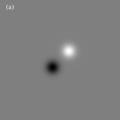
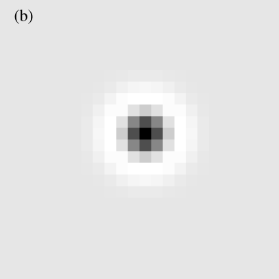
Figure 1: (a) Vertical magnetic field on the photosphere, (b) vertical current density distribution imposed in the positive polarity.

The bipolar vertical magnetic field component is simply given by a Gaussian distribution with the same full-width at half-maximum for both polarities of 15 Mm (see Fig. 1a). The maximum field strength is set to 2000 G. The considered field-of-view has dimensions 150 Mm$\times$150 Mm assuming a square pixel of 1 Mm². The separation between the two polarities is 50 Mm. The magnetic flux is balanced and the total unsigned magnetic flux is 7.1 10²¹ Mx. A typical bipolar magnetic field used in this study is depicted in Fig. 1a. The field-of-view is large enough to have no magnetic flux on the edges of the surface. We impose a ring distribution of current at the positive source of the form:

$$J_{z}(r)=2\leavevmode\nobreak\ J_{z0}\leavevmode\nobreak\ [r^{2}-C_{0}]\leavevmode\nobreak\ \exp{\left(-\frac{r^{2}}{\sigma^{2}}\right)},$$ (24)

where $r$ is measured from the centre of the source and $C_{0}$ is a constant which ensure a zero net current. We always take care to (i) keep a zero net current, and (ii) have enough pixels to describe the steep gradient between the positive and negative currents. A typical distribution used in this experiment is shown in Fig. 1b. We set $J_{z0}$ to 10 mA$\cdot$m^-2. To satisfy the Grad-Rubin boundary-value problem, the current distribution is defined in only one polarity. This equilibrium corresponds to a single twisted flux tube with an excess magnetic energy of 3% above the potential field.

3.2 Magnetic field strength

We first study the distribution of magnetic field strength with height for potential and nlff fields. We plot the average field strength as a function of height in Fig. 2. The average strength values start from 80 G at the photosphere and tend to zero. The rapid decrease of the field strength is due to the confinement of the twisted flux tube at a height lower than 30 Mm due to a separation between polarities of 50 Mm. There is a small departure of the nlff field values from the potential values due to the storage of magnetic energy in the corona associated with the twisted flux tube (see e.g, Régnier & Priest, 2007b).

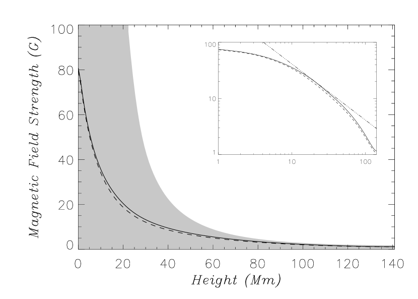
Figure 2: Average field strength as a function of height (Mm) for the nlff field (solid line) and the potential field (dashed line). The grey area is enclosed between the minimum and maximum field strengths at a given height. The log-log plot is drawn in the top-right corner. The dot-dashed line indicates the $z^{-1}$ decay of the field.

In Fig. 2, we also plot the log-log distribution of the average field strength with height in order to determine the shape of the decaying magnetic field. For both the potential and nlff fields, the average magnetic field strength decays rapidly from the photosphere up to about 20 Mm and then the rate of decline of the field strength reduces with a slope index greater than -1 as indicated by the dot-dashed line in the log-log plot of Fig. 2. We focus our interest on an index of -1 which corresponds to the typical slope of a dipolar field average on a surface. The whole curve is well fitted by a function of the following form:

$$\overline{B}(z)=B_{0}\exp\left[-\ln^{2}\left(\frac{z}{z_{0}}\right)\right]=B_{0}\left(\frac{z_{0}}{z}\right)^{\ln{(\frac{z}{z_{0}})}},$$ (25)

as deduced from the log-log plot, where $\overline{B}$ is the average field strength and $z$ the height ($B_{0}$ and $z_{0}$ being constants). Dere (1996) found that the magnetic field decay below 40 Mm is well described by an exponential decay. We will discuss these typical curves further in Section 5.

3.3 Alfvén speed

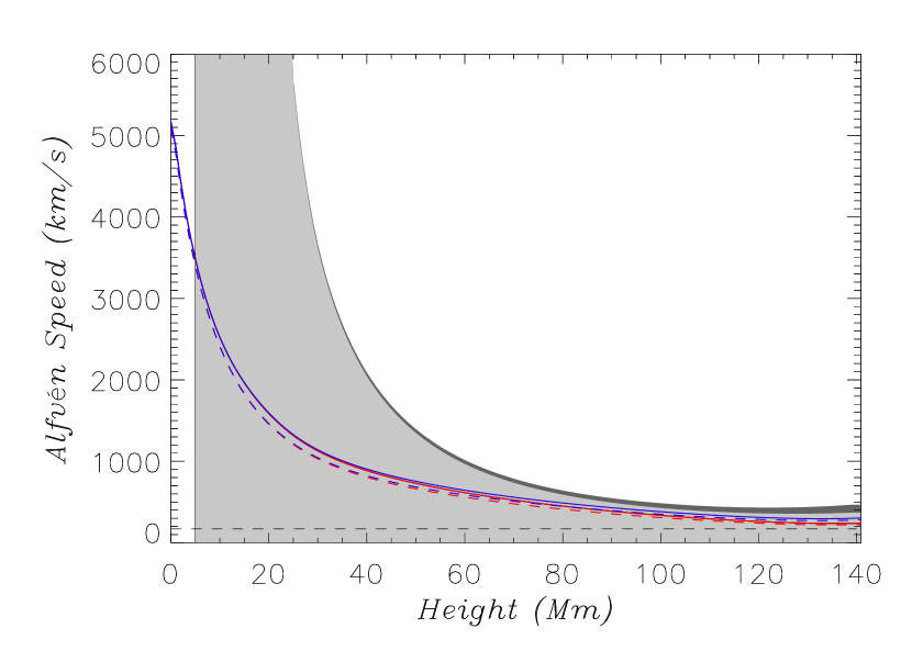
Figure 3: Average Alfvén speed (km$\cdot$s^-1) as a function of height (Mm) for $H=$ 50 Mm and $\rho_{0}=10^{9}$ cm^-3. Blue and red solid curves are from the nlff field for the constant and varying gravity models respectively. Blue and red dashed curves are from the potential field for the constant and varying gravity models respectively. The red and blue curves are very similar and almost superimposed. The dark and light grey areas indicate the spread of Alfvén speed values at a given height for the constant and varying gravity models respectively: only above 60 Mm, one can slightly notice the difference between the two gravity models.

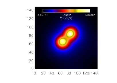
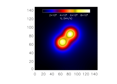
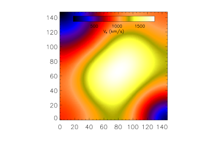
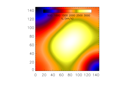
Figure 4: Dynamic range of the Alfvén speed at 10 Mm (top row) and 60 Mm (bottom row) for two sets of free parameters ($\rho_{0}$, $H$) in (cm^-3, Mm): (10⁹, 25), (10⁸, 50) from left to right.

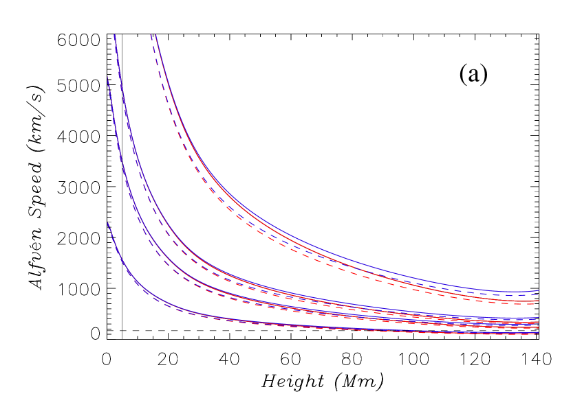
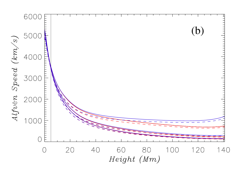
Figure 5: Average Alfvén speed (km$\cdot$s^-1) as a function of height (Mm) for the nonlinear force-free field (solid line) and the potential field (dashed line). (a): for $H=$ 50 Mm and $\rho_{0}=[5\leavevmode\nobreak\ 10^{9},10^{9},5\leavevmode\nobreak\ 10^{8},10^{8}]$ cm^-3 (from left to right); (b): for $H=[100,50,25]$ Mm (from left to right) and $\rho_{0}=10^{9}$ cm^-3. Red (resp. blue) curves are for the varying (resp. constant) gravity model.

We derive the Alfvén speeds from the model described above with $H=$ 50 Mm (1 MK) and $\rho_{0}=$ 10⁹ cm^-3. In Fig. 3, we plot the average Alfvén speed at a given height from both the potential field (dashed line) and the nonlinear force-free field (solid line). The Alfvén speed values are valid only above 5 Mm (vertical solid straight line). Under the force-free assumption, the plasma $\beta$ is considered to be much less than 1. The plasma $\beta$ can be expressed in terms of the Alfvén and sound speeds: $2c_{s}^{2}/\gamma v_{A}^{2}$. In an isothermal atmosphere, we then obtain a minimum value for the Alfvén speed:

$$v_{A,min}^{2}=2c_{s}^{2}.$$ (26)

As the sound speed is 120 km$\cdot$s^-1 for $H=50$ Mm, we plot $v_{A,min}=$ 170 km$\cdot$s^-1 in Fig. 3 and Fig. 5a (dashed straight line). The average Alfvén speed is similar for both gravity models in the case of the bipolar field. The curves are exactly the same up to a height $z=H$. Thus, we only report here the values for the constant gravity model. The average Alfvén speed decreases with height suggesting that the magnetic field decreases faster than the square root of the density with height. The Alfvén speed values range between 2400 km$\cdot$s^-1 at 10 Mm and 300 km$\cdot$s^-1 at 140 Mm. The scatter of the Alfvén speed (grey areas in Fig. 3) strongly depends on the height: a maximum value of 24000 km$\cdot$s^-1 at 10 Mm with a standard deviation of 3800 km$\cdot$s^-1, and a maximum value of 990 km$\cdot$s^-1 at 60 Mm with a standard deviation of 200 km$\cdot$s^-1 (see Fig. 4). By drawing the dynamic range of the Alfvén speed at different heights (see Fig. 4), we show that the Alfvén speed is larger where the field strength is larger whatever the density or the pressure scale-height: the two opposite polarities are clearly seen at 10 Mm and the loop top is seen at 60 Mm.

We now study the effects of two free parameters: the density at the base of the corona $\rho_{0}$ (see Fig. 5a) and the pressure scale-height $H$ (see Fig. 5b). In Fig. 5a, we plot the evolution of average Alfvén speed with height for several values of the density $\rho_{0}$ varying from 10⁸ to 5 10⁹ cm^-3. As the magnetic field is the same, the average Alfvén speed follows the density variations which can be seen from the values of the Alfvén speed at 5 Mm: 1560 km$\cdot$s^-1 for $\rho_{0}=5\leavevmode\nobreak\ 10^{9}$ cm^-3, 3500 km$\cdot$s^-1 for $\rho_{0}=10^{9}$ cm^-3, 4950 km$\cdot$s^-1 for $\rho_{0}=5\leavevmode\nobreak\ 10^{8}$ cm^-3 and 11070 km$\cdot$s^-1 for $\rho_{0}=10^{8}$ cm^-3. We note that there is a minimum of these curves at about 135 Mm. This minimum was also noticed by Lin (2002) but at about 0.5 R_⊙ ($\sim$ 350 Mm) for an isothermal atmosphere. From Eqn. (19), the minimum corresponds to the location where the variations of the gas pressure are becoming more important than those of the magnetic field (that does not mean that the plasma $\beta$ becomes greater than 1!). We conclude that this minimum is strongly related to the distribution of the magnetic field: from Eqn. 19, we deduce that the minimum of the curves is obtained for a constant gravitational field when the magnetic field satisfies

$$\frac{\partial B}{\partial z}=-\frac{B}{2H},$$ (27)

which depends only on the pressure scale-height. For a gravitational field varying with height, the minimum occurs where

$$\frac{\partial B}{\partial z}=-\frac{B}{2H}\left(\frac{R_{\odot}}{R_{\odot}+z}\right)^{2}.$$ (28)

We can already mention that Eqn. (27) is similar to the equation derived by Filippov & Den (2000) for the height of unstable prominences. In Fig. 5b, we plot the average Alfvén speed with height for several values of the pressure scale-height varying from 25 to 100 Mm (from 0.5 to 2 MK, resp.) giving a sound speed between 83 km$\cdot$s^-1 and 165 km$\cdot$s^-1, respectively. Therefore, the Alfvén speed curve for $H=$ 100 Mm is less than $v_{A,min}$ above 100 Mm, and the curve for $H=$ 25 Mm is way above $v_{A,min}$ whatever the height. The minimum of the curves is decreasing with height when $H$ decreases. The Alfvén speed values increase significantly when $H$ decreases: at 100 Mm, the Alfvén speed is 200 km$\cdot$s^-1 for $H=$ 100 Mm, 400 km$\cdot$s^-1 for $H=$ 50 Mm and 1000 km$\cdot$s^-1 for $H=$ 25 Mm.

From this study, we conclude that a density at the base of the corona of 10⁹ cm^-3 and a pressure scale-height of 50 Mm are a reasonable choice of parameters to model an isothermal corona. We will adopt these values in the following Sections.

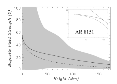
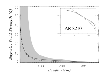
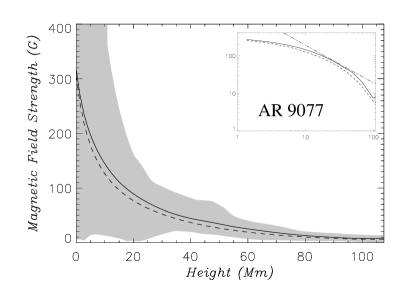
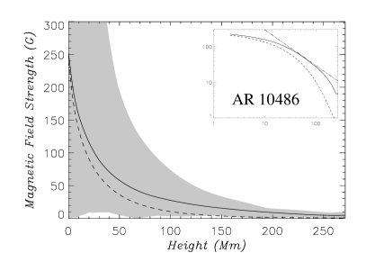
Figure 6: Average magnetic field strength as a function of height for the potential field (dashed line) and for the nonlinear force-free field (solid line). The grey area ranges from the minimum to the maximum field strength of the nonlinear force-free field. The log-log plots are drawn in the top-right corners. The dot-dashed line indicates the $z^{-1}$ decay of the field.

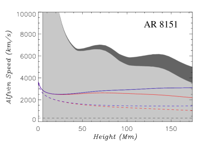
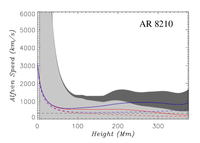
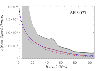
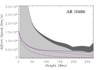
Figure 7: Same as Fig. 3 for different active regions: AR 8151 (top left), AR 8210 (top right), AR 9077 (bottom left), AR 10486 (bottom right).

4 Active regions

4.1 Magnetic field strength in active regions

Before computing the Alfvén speed, we study the changes of magnetic field strength depending on the nature of the observed active region and on the extrapolation model. We first compute the potential and nonlinear force-free magnetic fields associated with the four active regions described in Section 2.1. Then we derive the magnetic field strength average in an xy–plane as a function of height. In Fig. 6, we plot the average field strength for the potential field (dashed line) and the nonlinear force-free field (solid line). The grey area is the variation of field strength for the nonlinear force-free field at a given height.

For AR 8151 (Fig. 6 top left), the average nlff field strength ranges from 55 G on the photosphere to 9 G at 170 Mm. Assuming that the decrease of the field strength should be exponential, there is an excess in the values of the field strength between 40 Mm and 100 Mm where the twisted flux bundles are located (see Régnier & Amari, 2004; Régnier & Priest, 2007b).

For AR 8210 (Fig. 6 top right), the average nlff field strength varies from 45 G on the photosphere to small values above 300 Mm. The nlff curve (solid line) follows an exponential decay as for the potential field (dashed line). It is noticeable that the scatter of the field strength below 50 Mm is of about two orders of magnitude. Even if the storage of magnetic energy is focussed near the surface (Régnier & Priest, 2007b), the largest departure from potential occurs between 50 Mm and 300 Mm. Below 50 Mm, the average values of the nlff field strength are similar to the potential ones but the spatial distribution is different: the free magnetic energy above the potential field is only 2.5% of the total magnetic energy and the energy is stored near topological elements in the nlff field, as mentioned in Régnier & Priest (2007a, b).

For AR 9077 (Fig. 6 bottom left), the total magnetic flux on the photosphere is more important than for the above examples. The average field strength varies from 300 G on the photosphere to 90 G at 110 Mm. The average strength from the nlff field follows the same decay as for the potential field. The active region was observed after a X5.7 flare and exhibits post-flare loops. The variation of the field strength with height indicates very little storage of magnetic energy in the corona due to twisted flux tubes contrary to AR 8151.

For AR 10486 (Fig. 6 bottom right), the average field strength varies from 250 G on the photosphere to 5 G at 250 Mm. It is noticeable that the magnetic energy can be stored in the corona up to 150 Mm as seen by the departure from the potential field (dashed curve).

By studying the global properties of the magnetic field strength above several active regions, we conclude that:

• the main magnetic flux concentration occurs near the photosphere up to a height of 50 Mm;

• a significant amount of magnetic energy can be stored in the corona (between 50 and 150 Mm) in an active region with highly twisted flux bundles (AR 8151) or with a complex topology associated with a strong photospheric flux (AR 10486);

• the potential and nlff fields have different behaviours depending on the nature of the field: strong departure from the potential field for active regions with highly twisted flux tubes or complex topology associated with a high activity level, and small departure for active regions after a strong flare or with a complex topology not related to important flare activity.

As pointed out by Koutchmy (2004), there are few measurements of the magnetic field strength in the solar atmosphere. The above study shows that the average values at a given height strongly depend on the nature of the active region (the total magnetic flux and the distribution of polarities on the photosphere) and on the nature of the coronal magnetic field (potential or nlff fields). In Section 5 we will discuss the implications for different solar models.

Regarding the relationship between eruption and magnetic field decay, the log-log plots (see Fig. 6) show several interesting features:

• the $z^{-1}$ decay line is tangent to the curve of the nlff field at about 80 Mm for both active regions (AR 8151 and AR 10486) associated with an eruption causing a large-scale magnetic field reorganisation, whilst for a post-eruptive active region (AR 9077) and the one associated with confined flares (AR 8210), the $z^{-1}$ line is at about 20 Mm;

• the weak slope of the log-log plots below the $z^{-1}$ line indicates the strong influence of the current systems as in van Tend & Kuperus (1978).

The implications for eruption models are developed in Section 5.

4.2 Alfvén speed in solar active regions

We apply the above models to the active regions described in Section 2.1. To avoid confusion, we only report here the Alfvén speed values for the constant gravity model. In Fig. 7, we plot the average Alfvén speed values in the xy–plane as a function of height derived from the potential field (dashed curves) and nlff field (solid curves) for the different active regions. First, the average Alfvén speed at the base of the corona varies from 2–3000 km$\cdot$s^-1 for AR 8151 and AR 8210 to 13000 km$\cdot$s^-1 for AR 9077 and AR 10486. It is strongly related to the total magnetic flux of the active region on the photosphere. Above the coronal base, the variation of the Alfvén speed with height is greatly influenced by the nature of the field: the topology, the geometry of field lines and the effects of currents.

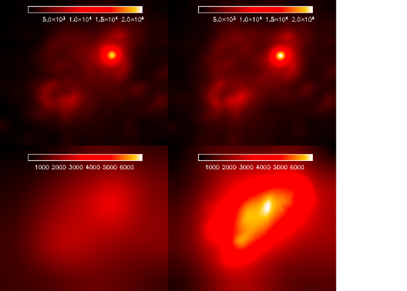
Figure 8: Alfvén speed dynamic range in AR 8151 for the potential field (left column) and the nonlinear force-free field (right column) at two different heights, 10 Mm (top) and 60 Mm (bottom).

For AR 8151, the Alfvén speeds in the nlff field can reach up to 52000 km$\cdot$s^-1 near the base of the corona (for an average value of 3000 km$\cdot$s^-1). Then the maximum Alfvén speed values decrease to 6000 km$\cdot$s^-1 at 50 Mm to finally reach the value of 5000 km$\cdot$s^-1 above 150 Mm. The evolution of the average values is almost constant at 3000 km$\cdot$s^-1. Nevertheless there is a minimum of Alfvén speed of 2500 km$\cdot$s^-1 at 25 Mm. This result is consistent with Warmuth & Mann (2005). According to Régnier & Priest (2007b), the minimum is below the height where the twisted flux tubes are located and the magnetic energy is deposited in this active region. The evolution of the average speeds in the potential field (dashed curve) is strictly decreasing from 2500 km$\cdot$s^-1 to 1500 km$\cdot$s^-1. Note that according to Section 3, the average speeds should increase above 170 Mm when the density dominates. Both potential and nlff average speed curves are above the $\beta<1$ limit (dashed line). Even if the average values of the Alfvén speed for the potential and nlff fields are not far from each other in the low corona, there is a factor of about 2 difference above 80 Mm. In Fig. 8, we draw the dynamic range of Alfvén speed at two different heights (top: 10 Mm, bottom: 60 Mm) for both potential (left) and nlff (right) fields. At both heights and for both models, the greater is the magnetic field strength, the larger is the Alfvén speed. Even if the dynamic range is similar for the potential and nlff fields at 10 Mm, the Alfvén speed varies by a factor of 2 at 60 Mm due to the presence of twisted flux bundles along the polarity inversion line. The average Alfvén speed decreases more rapidly for the varying gravity model: at a height of 150 Mm, the average Alfvén speed is 2400 km$\cdot$s^-1 for a varying gravity and 3000 km$\cdot$s^-1 for a constant gravity.

Figure 9: Alfvén speed dynamic range in AR 8210 for the potential field (left column) and the nonlinear force-free field (right column) at two different heights, 10 Mm (top) and 60 Mm (bottom).

For AR 8210, the maximum Alfvén speed at the base of the corona is about 70000 km$\cdot$s^-1. Even if the total magnetic flux is comparable to the flux of AR 8151, the maximum field strength is larger in the main sunspot of AR 8210 (Régnier & Canfield, 2006) which explains the larger value of the maximum Alfvén speed. The average speed for the nlff field decreases rapidly from the base of the corona to about 70 Mm from 2200 km$\cdot$s^-1 to 600 km$\cdot$s^-1. The fast decrease is explained by the nature of the magnetic configuration: the confined magnetic field in the active region, and the storage of magnetic energy in the low corona (see Régnier & Canfield, 2006). The average speed for the potential field follows the same fast decrease below 70 Mm before reaching a minimum at about 150 Mm. Above this height, the average speed slowly increases when the density dominates the field strength. At 100 Mm, the average speed for the nlff field (potential resp.) is about 650 km$\cdot$s^-1 (400 km$\cdot$s^-1 resp.) which is indeed of factor of 1.5 more for the nlff field. The dynamic range of the Alfvén speed is depicted in Fig. 9. There are very few changes between the dynamic range images at a given height. We then suggest that the complex topology of AR 8210 does not significantly influence the Alfvén speed distribution. This conclusion is also supported by the fact that the magnetic energy is deposited near the photospheric boundary and not in the corona. Since the average Alfvén speed decreases faster for the varying gravity model, the Alfvén speed becomes less than the coronal sound speed at about 300 Mm, whilst the Alfvén speed stays above the plasma $\beta=1$ limit for the constant gravity model.

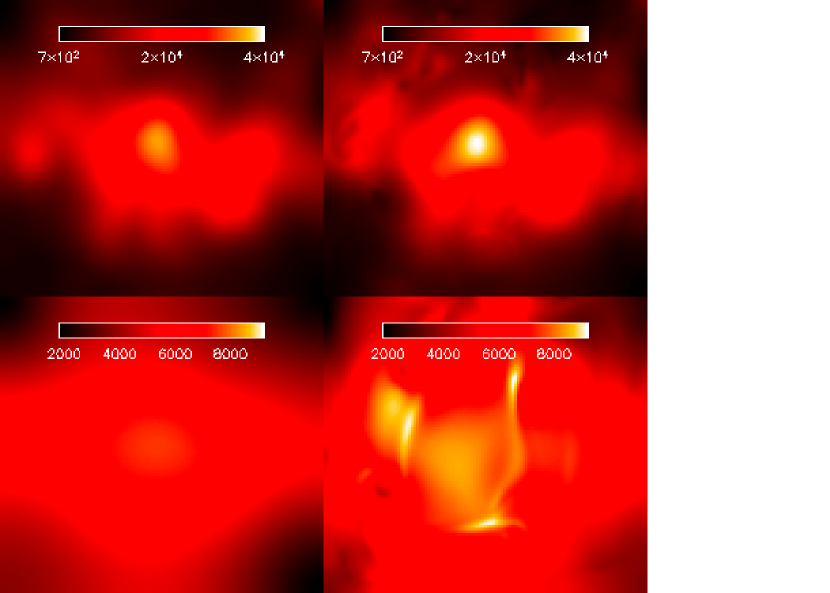
Figure 10: Alfvén speed dynamic range in AR 9077 for the potential field (left column) and the nonlinear force-free field (right column) at two different heights, 10 Mm (top) and 60 Mm (bottom).

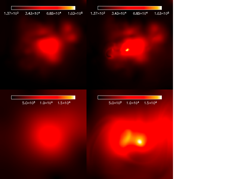
Figure 11: Alfvén speed dynamic range in AR 10486 for the potential field (left column) and the nonlinear force-free field (right column) at two different heights, 10 Mm (top) and 60 Mm (bottom).

For AR 9077, the total magnetic flux included in the field-of-view is larger than for the previous two examples. Therefore, even if the maximum Alfvén speed at the base of the corona is moderate ($\sim$ 46000 km$\cdot$s^-1), the average speed is relatively large (13000 km$\cdot$s^-1). Both average curves for the potential and nlff field are rapidly and strictly decreasing towards 1500 km$\cdot$s^-1. Contrary to the previous example, there is no evidence of storage of energy in the middle corona. The strong flare and the CME associated with this active region are related to a complex topology and the mass supply is provided by a low filament on the side of the active region (e.g., Zhang, 2002). The reconstructed active region is performed from a magnetogram recorded after the flare. As suggested by Fig. 10, the dynamic ranges are quite different from one model to another, whatever the altitude we look at, even if the Alfvén speed values are comparable. Therefore the post-eruptive configuration is strongly influenced by the electric currents flowing along field lines despite a magnetic geometry which looks similar to potential. For both gravity models, the average Alfvén speed curves are similar indicating that, during this relaxation phase, gravity does not greatly influence the magnetic field and the plasma.

For AR 10486, the maximum Alfvén speed at the base of the corona is estimated to be 130000 km$\cdot$s^-1, which is about one-third of the speed of light. The average speed for both potential and nlff fields is about 13000 km$\cdot$s^-1. The average speed for the nlff field is decreasing rapidly from 13000 km$\cdot$s^-1 at 5 Mm to 6000 km$\cdot$s^-1 at 50 Mm and then reaches an almost constant value of 5000 km$\cdot$s^-1. In the view of the previous examples, we interpret this fact as a consequence of the storage of magnetic energy in the corona at a height of about 50 Mm either by twisted flux tubes or by sheared arcades. Following Régnier & Fleck (2004), the existence of sheared arcades in a complex topology is confirmed. The effects of the transverse field components and so of the electric currents are shown in Fig. 11. The location of strong magnetic field strength is different from one model to another showing the complex distribution of the magnetic field on the photosphere (e.g., Régnier & Fleck, 2004; Mandrini et al., 2006). The Alfvén speed for the constant gravity model is almost twice the value for the varying gravitational field high in the corona.

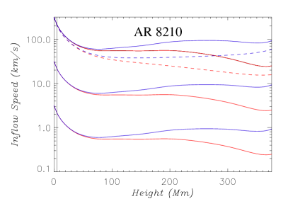
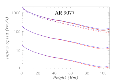
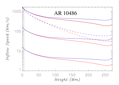
Figure 12: Average inflow speeds as a function of height for the nonlinear force-free field (solid line) and potential field (dashed line), with a reconnection rate $M_{e}$ varying from 10^-3 to 10^-1. Red (resp. blue) curves are for the varying (resp. constant) gravity model.

5 Discussions and Conclusions

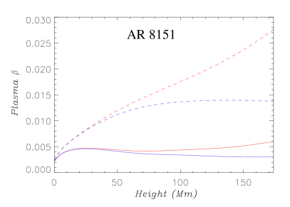
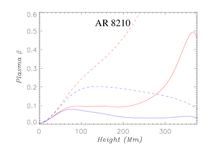
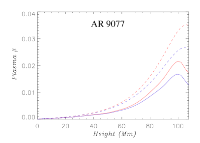
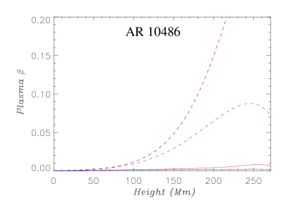
Figure 13: Plasma $\beta$ for the nonlinear force-free field (solid line) and the potential field (dashed line) as a function of height for four active regions. Red (resp. blue) curves are for the varying (resp. constant) gravity model.

In this paper, we address two questions related to the global properties of the magnetic field and the plasma in the corona:

• How does the magnetic field strength and Alfvén speed vary with height in the solar corona?

• What can we learn from the estimate of the coronal Alfvén speed for some key solar physics problems (coronal heating, magnetic reconnection, wave propagation, initiation and development of CMEs)?

In order to tackle the above questions, we have developed a method to determine the plasma properties in a magnetic field above active regions. We assume that an active region can be modelled in two steps: a nonlinear force-free equilibrium for the magnetic field, and a hydrostatic equilibrium between pressure and gravity forces describing the plasma properties. To solve the latter equation, the corona is assumed here to be isothermal with either a constant gravity or a gravitational field varying with height.

In Sections 3.2 and 4.1, we investigated the evolution of the average field strength with height. Interestingly, the log-log plots showed that the decay of the magnetic field with height does not follow a power law, even for a potential field. This fact suggests that the decay of the field strength is strongly influenced by the geometry of the field (e.g., toroidal geometry for the bipolar field), by the distribution of electric currents and their typical height of influence, and by the complexity of the magnetic distribution on the photosphere for active regions. This is a well-known property of the magnetic field. Based on the data reported by Poletto et al. (1975), van Tend & Kuperus (1978) plotted the measured magnetic field strength as a function of height for three different active regions and assuming current-free magnetic configurations. They obtained similar curves to those shown in this paper in which the log-log plot can be fitted by a parabola. In addition, they fitted the distribution of field strength by two power laws of index -1 and -3 suggested by their theoretical work: -1 for a line current along the inversion line of the magnetic field and -3 for a dipolar potential field decay. van Tend & Kuperus (1978) concluded that (i) the electric currents strongly influence the magnetic configuration when the power law index is less than -1, (ii) above a certain height the magnetic field decays rapidly (probably with a power law index of -3). More importantly, the authors concluded that, if the magnetic field below the $z^{-1}$ decay is decaying with a power law index less than -1, then the configuration is stable. This condition can be compared with the conditions required to trigger a kink instability (e.g., Hood & Priest, 1981) or a torus instability (Kliem & Török, 2006). Recently, Liu (2008) investigated the evolution of the magnetic field strength with height and compared with the nature of the eruptive phenomenon. He derived the magnetic field from a large-scale potential field extrapolation based on the PFSS model (Potential Field Source Surface, e.g., Schatten et al. 1969). For heights between 42 Mm and 140 Mm, the power law index is about -1.5 whatever the onset mechanism. Combined with our study, this result suggests that the behaviour of the magnetic field in the low atmosphere plays the main role in triggering flares and CMEs, and also that electric currents flowing along field lines as in the nlff model affect strongly the power law index and therefore the stability of the magnetic configuration.

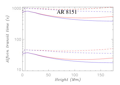
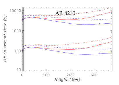
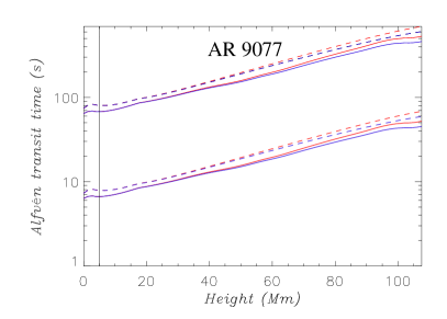
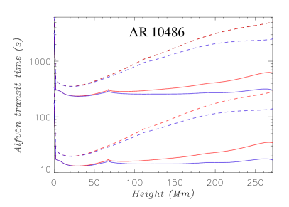
Figure 14: Average Alfvén transit time for the potential (dashed line) and nonlinear force-free (solid line) fields using as typical scale the pressure scale-height $H$ (bottom curves) or the length of a semi-circular loop with a diameter of the scale of the computational box (top curves). Red (resp. blue) curves are for the varying (resp. constant) gravity model.

5.1 Reconnection rate

As mentioned in Section 1, the Alfvén speed is an important parameter in understanding the magnetic reconnection processes. The reconnection is characterised by the reconnection rate (or external Alfvén Mach number) as follows:

$$M_{e}=\frac{v_{i}}{v_{A}},$$ (29)

where $v_{i}$ is the inflow speed. This definition does not depend on the nature of the diffusion region where the magnetic reconnection occurs. To distinguish between different regimes of reconnection, the magnetic Reynolds number is introduced as follows:

$$R_{me}=\frac{\eta}{L_{e}v_{A}},$$ (30)

where $\eta$ is the magnetic diffusivity, and $L_{e}$ is a typical length of the diffusion region (e.g., Priest & Forbes, 2000). If $R_{me}^{-1}<M_{e}<R_{me}^{-1/2}$, we have a slow reconnection regime of the Sweet-Parker type. If $M_{e}>R_{me}^{-1/2}$, the reconnection regime is fast such as in the Petschek (1964) model. For a typical astrophysical plasma, the reconnection rate in the fast regime is in the range 0.01 to 0.1. The square of the reconnection rate is also the ratio of kinetic energy to magnetic energy of the inflow region assuming that the diffusion region is small enough to have the same field strength in the inflow and outflow regions. For a given inflow speed, the higher is the magnetic energy stored in the region, the smaller is the reconnection rate.

If we assume that the reconnection rate is between 10^-3 and 10^-1 (see e.g., Narukage & Shibata, 2006), we can infer the inflow speed required to trigger the reconnection. The results for the four studied active regions are summarized in Fig. 12, where we plot the inflow speed as a function of height for different reconnection rates ($M_{e}=0.1,0.01,0.001$) for both potential (dashed curves) and nlff (solid curves) fields. The variation with height of the inflow speed is consistent with the variation of the Alfvén speed as described in Fig. 7. From these curves, we can deduce a threshold on the reconnection rate in order to obtain inflow speeds in agreement with observations (e.g., Narukage & Shibata, 2006; Nagashima & Yokoyama, 2006). For instance, if a reconnection process occurs in AR 8151, the reconnection rate should be of the order or below 0.01 which gives typical inflow speeds below 50 km$\cdot$s^-1.

We also note that the minimum of the inflow speed or Alfvén speed (see Section 3) is the location in the low corona where the reconnection process is more likely to happen. The conclusion is valid in a statistical sense because we only consider average values of the inflow speed and because, in order for it to occur, the reconnection process needs a particular magnetic topology and a diffusion region which are beyond the scope of this article.

5.2 Coronal plasma $\beta$

An important quantity in plasma physics is the plasma $\beta$, the ratio of the gas pressure to the magnetic pressure. When $\beta\ll 1$, the plasma is dominated by the magnetic field. Nevertheless, the plasma $\beta$ in the solar atmosphere varies greatly with height (Gary, 2001). In addition, we note that the plasma $\beta$ varies from one structure to another and even coronal structures, such as filaments, can have $\beta\geq 1$. As mentioned in Section 3, the plasma $\beta$ can be expressed as follows:

$$\beta=\frac{2\leavevmode\nobreak\ c_{s}^{2}}{\gamma v_{A}^{2}}$$ (31)

for an isothermal atmosphere ($\gamma=1$). In Fig. 13, we plot the variation of the average plasma $\beta$ with height for the four active regions described in Section 2.1. For both potential and nlff models, the plasma $\beta$ is less than 1. This result is consistent with the typical nature of the coronal active region magnetic field. The plasma $\beta$ is larger for the potential field because the average Alfvén speed decreases with height more rapidly than for the nlff field. The maximum of the plasma $\beta$ is located at the same height as the minimum of Alfvén speed (see Section 3.3) and also satisfies Eqn. (27). The plasma $\beta$ tends to zero for a constant gravitational field, whilst it increases towards 1 for the varying gravity model. The latter is then in agreement with plasma $\beta$ measurements reported by Gary (2001).

5.3 Average Alfvén transit time

The Alfvén transit time is an important quantity for the propagation of Alfvén waves and for the relaxation of a magnetic configuration. In this study of global properties of Alfvén speeds, we derive the average Alfvén transit time associated with two different lengths:

$$\tau_{A}^{(H)}=\frac{H}{v_{A}}$$ (32)

and

$$\tau_{A}^{(\pi L)}=\frac{\pi L}{v_{A}},$$ (33)

where $v_{A}$ is the Alfvén speed, $H$ is the pressure scale-height and $L$ is the length of the computational box. We suppose $\tau_{A}^{(H)}$ (resp. $\tau_{A}^{(\pi L)}$) is a minimum (resp. maximum) of the Alfvén transit time. The larger the Alfvén transit time is, the more stable the equilibrium is. In Fig. 14, we plot the different Alfvén transit times for the four active regions. At the base of the corona (5 Mm), the maximum Alfvén time is 750s for AR 8151, 3600s for AR 8210, 70s for AR 9077, 300s for AR 10486. These results mean that the most stable active region is AR 8210 associated with confined C-class flares, and the least stable one is AR 9077 exhibiting post-flare loops. It is worth noticing that the average Alfvén transit time is an interesting quantity only when discussing the global or statistical properties of magnetic configurations. A more appropriate quantity is the Alfvén transit time along a single field line which is beyond the scope of this article. Of importance for MHD modelling, the Alfvén transit time along field lines is not a constant with height which makes it difficult to estimate the scaling of the time evolution with this quantity.

Despite the simple assumptions of this model, we have derived interesting properties of the Alfvén speed in the solar corona. In a forthcoming paper, we will focus on the properties of individual field lines.