Wave dynamics of phantom scalar perturbation in the background of Schwarzschild black hole

Abstract

Abstract

Using Leaver’s continue fraction and time domain method, we investigate the wave dynamics of phantom scalar perturbation in the background of Schwarzschild black hole. We find that the presence of the negative kinetic energy terms modifies the standard results in quasinormal spectrums and late-time behaviors of the scalar perturbations. The phantom scalar perturbation in the late-time evolution will grow with an exponential rate.

Many observations confirm that our universe is undergoing an accelerated expansion. In order to explain this observed phenomena, the universe is supposed to be filled with dark energy within the framework of Einstein’s general relativity. Dark energy is an exotic energy component with negative pressure and constitutes about $72\%$ of present total cosmic energy. The simplest explanation for dark energy is the cosmological constant 1a , which is a term that can be added to Einstein’s equations. This term acts like a perfect fluid with an equation of state $\omega_{x}=-1$, and the energy density is associated with quantum vacuum. Although this interpretation is consistent with observational data, it suffers the coincidence problem, namely, “why are the vacuum and matter energy densities of precisely the same order today?”. Therefore the dynamical scalar fields, such as quintessence 2a , k-essence 3a and phantom field 4a , have been put forth as an alternative of dark energy.

The phantom field model is an interesting candidate for dark energy since it has some peculiar properties. This field has a negative kinetic energy and so that the null energy condition is violated and the equation of state $\omega_{x}$ of dark energy less than $-1$. The super negative equation of state is favored by recent precise observational data involving CMB, Hubble Space Telescope, type Ia Supernova, and 2dF data sets 5a . The dynamical properties of the phantom field in the cosmology has been investigated in the last years 6a1 ; 6a11 ; 6a2 ; 6a3 ; 6a4 ; 6a5 ; 6a6 ; 6a7 . It shows that the energy density increases with the time and approaches to infinity in a finite time 6a1 . In other words, the universe dominated by phantom energy will blow up incessantly and arrive at a big rip finally, which is a future singularity with a strong exclusive force so that anything in the universe including the large galaxies will be torn up. Recently, many efforts have been working to avoid the big rip 7b . It has argued that if one considers the effects from loop quantum gravity, this future singularity will be disappeared in the universe lc3 ; lg4 ; lg6 ; lg7 .

It is of interest to extend the study of dynamical evolution of the phantom field to black hole spacetime in various gravity theories, since this could help us to obtain the connection between dark energy and black hole. The dynamical evolution of usual scalar field perturbation has been studied for the last few decades (for a review, see qn1 ; qn2 ; qn3 ). It is well known that a static observer outside a black hole can indicate three successive stages of the wave evolution. The first one is that the exact shape of the wave front depends on the initial pulse. This stage is followed by a quasinormal ringing, which describes the damped oscillations under perturbations in the surrounding geometry of a black hole with frequencies and damping times of the oscillations entirely fixed by the black hole parameters. It is widely believed that the quasinormal modes carry characteristic fingerprint of a black hole and can offer a direct way to identify the black hole existence. Detection of these quasinormal modes is expected to be realized through gravitational wave observation in the near future qn1 ; qn2 . Apart from the potential astrophysical interest, quasinormal modes could also serve as a tool to test ground of fundamental physics. It has been argued that the study of QNM can help us get deeper understandings of the AdS/CFT qn3 ; qn4 , dS/CFT qn5 correspondences, loop quantum gravity qn6 and also the phase transition of black holes qn7 . In this letter, we treat the phantom field as an external perturbation and examine whether there exists some new feature in the dynamical evolution of phantom scalar field in a black hole spacetime.

In the curve spacetime, the action of the phantom scalar field with the negative kinetic energy term is

$$S=\int d^{4}x\sqrt{-g}\bigg{[}-\frac{R}{16\pi G}-\frac{1}{2}\partial_{\mu}\psi\partial^{\mu}\psi-V(\psi)\bigg{]}.$$ (1)

Here we take metric signature $(+---)$. The usual “Mexican hat” symmetry breaking potential has the form

$$V(\psi)=-\frac{1}{2}\mu^{2}\psi^{2}+\frac{\kappa}{4}\psi^{4},$$ (2)

where $\mu$ is the mass of the scalar field and $\kappa$ is the coupling constant. In general, the presence of the phantom scalar field will change the structure of the black hole spacetime phso1 . Here we just treat it as an external perturbation and suppose it does not affect the metric of the background. Meanwhile we only consider the case $\kappa=0$ for conveniently, namely, the potential has the form $V(\psi)=-\frac{1}{2}\mu^{2}\psi^{2}$. The wave dynamics of usual scalar perturbations with this type of the potential form has been extensively investigated in the various black holes spacetime ml1 ; ml2 .

Varying the action with respect to $\psi$, we obtain the wave equation for phantom scalar field in the curve spacetime

$$\frac{1}{\sqrt{-g}}\partial_{\mu}(\sqrt{-g}g^{\mu\nu}\partial_{\nu})\psi-\mu^{2}\psi=0.$$ (3)

Comparing the Klein-Gordon equation of usual massive scalar field, we find the unique difference in equation (3) is that the sign of the mass term $\mu^{2}$ is negative, which will yield the peculiar dynamical evolution of the phantom perturbation in the black hole spacetime.

Let us now to consider the case of a Schwarzschild black hole spacetime, whose metric in the standard coordinate can be described by

$$ds^{2}=(1-\frac{2M}{r})dt^{2}-(1-\frac{2M}{r})^{-1}dr^{2}-r^{2}(d\theta^{2}+\sin^{2}\theta d\phi^{2}).$$ (4)

Separating $\psi=e^{-i\omega t}R(r)Y_{lm}(\theta,\phi)/r$, we can obtain the radial equation for the scalar perturbation in the Schwarzschild black hole spacetime

$$\frac{d^{2}R(r)}{dr^{2}_{*}}+[\omega^{2}-V(r)]R(r)=0,$$ (5)

where $r_{*}$ is the tortoise coordinate (which is defined by $dr_{*}=\frac{r}{r-2M}dr$) and the effective potential $V(r)$ reads

$$V(r)=\bigg{(}1-\frac{2M}{r}\bigg{)}\bigg{(}\frac{l(l+1)}{r^{2}}+\frac{2M}{r^{3}}-\mu^{2}\bigg{)}.$$ (6)

Obviously, as $\mu=0$ the radial equation of phantom scalar field reduce to that of usual massless scalar field. In the case $\mu\neq 0$, the effective potential $V(r)$ vanishes at the event horizon and approaches to a negative constant $-\mu^{2}$ at the spatial infinity. This is different from that of usual massive scalar perturbation. Moreover, from figure (1), one can see that as the mass $\mu$ increases the effective potential $V(r)$ for the phantom scalar perturbation decreases and for the usual one increases. This implies the wave dynamics of the phantom scalar perturbation possesses some different properties from that of the usual scalar perturbation.

Figure 1: Variety of the effective potential $V(r)$ with $r$ for different $\mu$. The left for phantom scalar field and the right for normal scalar field. Here $l=0$ and $M=0.5$.

We are now in a position to apply the continue fraction method Leaver and calculate the fundamental quasinormal modes ($n=0$) of phantom scalar perturbation in the Schwarzschild black hole. From equation (6), we know that the boundary conditions on the wave function $R(r)$ have the form

$$R(r)=\bigg{\{}\begin{array}[]{lll}(r-1)^{-i\omega},\;\;\;\;\;\;\;\;\;\;\;\;r\rightarrow 1,\\ \\ r^{\frac{i(\chi^{2}+\omega^{2})}{2\chi}}e^{i\chi r},\;\;\;\;\;\;\;\;\;r\rightarrow\infty,\end{array}$$ (10)

where we set $2M=1$ and $\chi=\sqrt{\omega^{2}+\mu^{2}}$. A solution to Eq.(5) that has the desired behavior at the boundary can be written as

$$R(r)=r^{i(\chi+\omega)-\frac{i\mu^{2}}{2\chi}}(r-1)^{-i\omega}e^{i\chi r}\sum_{n=0}^{\infty}a_{n}\bigg{(}\frac{r-1}{r}\bigg{)}^{n}.$$ (11)

The sequence of the expansion coefficients $\{a_{n}:n=1,\;2,\;....\}$ is determined by a three-term recurrence relation staring with $a_{0}=1$:

$$\alpha_{0}a_{1}+\beta_{0}a_{0}=0,$$

$$\alpha_{n}a_{n+1}+\beta_{n}a_{n}+\gamma_{n}a_{n-1}=0,\;\;\;\;\;\;n=1,\;2,\;\ldots.$$ (12)

The recurrence coefficient $\alpha_{n}$, $\beta_{n}$ and $\gamma_{n}$ are given in terms of $n$ and the black hole parameters by

$$\alpha_{n}=n^{2}+(C_{0}+1)n+C_{0},$$

$$\beta_{n}=-2n^{2}+(C_{1}+2)n+C_{3},$$

$$\gamma_{n}=n^{2}+(C_{2}-3)n+C_{4}-C_{2}+2,$$ (13)

and the intermediate constants $C_{n}$ are defined by

$$C_{0}=1-2i\omega,$$

$$C_{1}=-4+i(4\omega+3\chi)+\frac{i\omega^{2}}{\chi},$$

$$C_{2}=3-i(2\omega+\chi)-\frac{i\omega^{2}}{\chi},$$

$$C_{3}=\bigg{(}\frac{\omega+\chi}{\chi}\bigg{)}\bigg{[}(\omega+\chi)^{2}+\frac{i(\omega+3\chi)}{2}\bigg{]}-l(l+1)-1,$$

$$C_{4}=-\bigg{[}\frac{(\omega+\chi)^{2}}{2\chi}+i\bigg{]}^{2}.$$ (14)

If the boundary condition (10) is satisfied and the series in (11) converge for the given $l$, the frequency $\omega$ is a root of the continued fraction equation

$$\beta_{n}-\frac{\alpha_{n-1}\gamma_{n}}{\beta_{n-1}-\frac{\alpha_{n-2}\gamma_{n-1}}{\beta_{n-2}-\alpha_{n-3}\gamma_{n-2}/...}}=\frac{\alpha_{n}\gamma_{n+1}}{\beta_{n+1}-\frac{\alpha_{n+1}\gamma_{n+2}}{\beta_{n+2}-\alpha_{n+2}\gamma_{n+3}/...}}.$$ (15)

This equation is impossible to be solved analytically. But we can rely on the numerical calculation to obtain the quasinormal frequencies for phantom scalar perturbations in the Schwarzschild black hole spacetime.

$\mu$	$l=0$	$l=1$	$l=2$
0	0.220910-0.209791i	0.585872-0.19532i	0.967288-0.193518i
0.1	0.223315-0.227501i	0.579967-0.200625i	0.962955-0.195599i
0.2	0.228479-0.269382i	0.562925-0.217049i	0.949962-0.201995i
0.3	0.232013-0.321298i	0.537016-0.245696i	0.928354-0.213175i

Table 1: The fundamental ($n=0$) quasinormal frequencies of phantom scalar field in the Schwarzschild black hole spacetime.

Figure 2: Change of the real part quasinormal frequencies ($n=0$) for the phantom scalar perturbations with the parameter $\mu$ for fixed $l$.

Figure 3: Change of the imaginary part quasinormal frequencies ($n=0$) for the phantom scalar perturbations with the parameter $\mu$ for fixed $l$.

In table I, we list the fundamental quasinormal frequencies of phantom scalar perturbation field for fixed $l=0$, $l=1$ and $l=2$ in the Schwarzschild black hole spacetime. From the table I and figures (1) and (2), we find that with the increase of the mass $\mu$ the real parts increase for $l=0$ and decrease for $l=1$ and $l=2$. The absolute value of imaginary parts for all $l$ increase, which can be explained by that the bigger $\mu$ leads to lower peak of the potential and thus it is easier for the wave to be absorbed into the black hole. The dependence of quasinormal modes on the mass $\mu$ is different from that of the usual scalar field since their effective potentials are quite a different in the black hole spacetime.

Now we will extend to study the late-time behavior of phantom scalar perturbations in the Schwarzschild black hole spacetime by using of the time domain method T1 .

Adopting the null coordinates $u=t-r_{*}$ and $v=t+r_{*}$, the wave equation

$$-\frac{\partial^{2}\psi}{\partial t^{2}}+\frac{\partial^{2}\psi}{\partial r_{*}^{2}}=V(r)\psi,$$ (16)

can be recast as

$$4\frac{\partial^{2}\psi}{\partial u\partial v}+V(r)\psi=0,$$ (17)

The two-dimensional wave equation (17) can be integrated numerically, using for example the finite difference method suggested in T1 . Using Taylor’s theorem, it is discretized as

$$\psi_{N}=\psi_{E}+\psi_{W}-\psi_{S}-\delta u\delta vV(\frac{v_{N}+v_{W}-u_{N}-u_{E}}{4})\frac{\psi_{W}+\psi_{E}}{8}+O(\epsilon^{4})=0,$$ (18)

where the points $N$, $S$, $E$ and $W$ from a null rectangle with relative positions as: $N$: $(u+\delta u,v+\delta v)$, $W$: $(u+\delta u,v)$, $E$: $(u,v+\delta v)$ and $S$: $(u,v)$. The parameter $\epsilon$ is an overall grid scalar factor, so that $\delta u\sim\delta v\sim\epsilon$. Considering that the behavior of the wave function is not sensitive to the choice of initial data, we set $\psi(u,v=v_{0})=0$ and use a Gaussian pulse as an initial perturbation, centered on $v_{c}$ and with width $\sigma$ on $u=u_{0}$ as

$$\psi(u=u_{0},v)=\text{exp}[-\frac{(v-v_{c})^{2}}{2\sigma^{2}}].$$ (19)

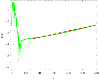
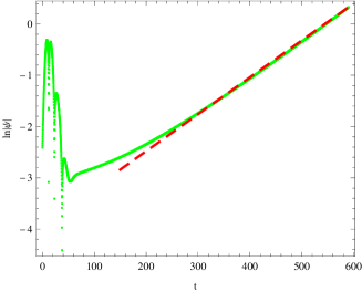
Figure 4: The late-time behaviors of the phantom scalar perturbations for fixed $l=0$, the left and the right are for $\mu=0.01$ and $0.02$, respectively. The dashed line denotes the function $\ln\psi\sim\alpha\mu t-4l-\beta$. We set the numerical constants $\alpha=0.27$, $\beta=3.93$ in the left figure and $\alpha=0.36$, $\beta=3.92$ in the right one. The constants in the Gauss pulse (19) $v_{c}=10$ and $\sigma=3$.

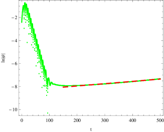
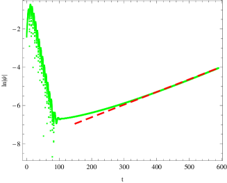
Figure 5: The late-time behaviors of the phantom scalar perturbations for fixed $l=1$, the left and the right are for $\mu=0.01$ and $0.02$, respectively. The dashed line denotes the function $\ln\psi\sim\alpha\mu t-4l-\beta$. We set the numerical constants $\alpha=0.20$, $\beta=4.32$ in the left figure and $\alpha=0.32$, $\beta=3.84$ in the right one. The constants in the Gauss pulse (19) $v_{c}=10$ and $\sigma=3$.

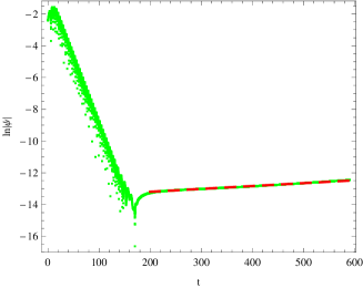
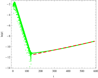
Figure 6: The late-time behaviors of the phantom scalar perturbations for fixed $l=2$, the left and the right are for $\mu=0.01$ and $0.02$, respectively. The dashed line denotes the function $\ln\psi\sim\alpha\mu t-4l-\beta$. We set the numerical constants $\alpha=0.18$, $\beta=5.55$ in the left figure and $\alpha=0.28$, $\beta=4.30$ in the right one. The constants in the Gauss pulse (19) $v_{c}=10$ and $\sigma=3$.

Here we confirm numerically the peculiar properties in late-time evolution of phantom scalar perturbations in the Schwarzschild black hole spacetime. In figures (4), (5) and $(6)$, we plot the evolutions of the phantom scalar perturbations for fixed $l=0$, $l=1$ and $l=2$, respectively. Unlike the usual massive scalar perturbations, the phantom scalar field after undergoing the quasinormal modes stage does not decay but grow with the time. The asymptotic behaviors of wave function for the phantom scalar field in the Schwarzschild black hole spacetime can be fitted best by

$$\psi\sim e^{\alpha\mu t-4l-\beta},$$ (20)

where $\alpha$ and $\beta$ are two numerical constant. It means that the phantom scalar perturbation grows with exponential rate in the late-time evolution. This behavior can be attributed to that the effective potential is negative at the spatial infinity shown in fig.(1), which implies that the wave outside the black hole gains energy from the spacetime. For the larger $\mu$, the scalar perturbation grows more faster since the larger $\mu$ corresponds to more negative potential. It is quite different from that of the usual massive scalar perturbations in a black hole spacetime which decay with the oscillatory inverse power-law behavior $t^{-\gamma}\sin{\mu t}$ ml1 ; ml2 . Moreover, the growing modes of the late-time tails caused by the negative effective potential was also observed in bwr .

The exponential growth of the phantom scalar perturbation in the late-time evolution also means that it is unstable in the black hole spacetime and its energy density will increase with the time, which is similar to that of in the Einstein cosmology. Our result also agrees with that obtained in the phantom energy accretion of black hole Eph , where the black hole mass will be decreased and the energy density of the phantom will increase.

In summary we examine the wave dynamics of the phantom scalar perturbation in the background of Schwarzschild black hole. Our results show that due to the presence of the negative kinetic energy, the properties of the wave dynamics of phantom scalar perturbation are different from that of the usual massive scalar field. In the late-time evolution the phantom field does not decay but instead grows with an exponential rate. It would be of interest to generalize our study to other black hole spacetimes, such as rotating black hole and stringy black holes etc. Work in this direction will be reported in the future.

- (1) S. Weinberg, Rev. Mod. Phys. 61 (1989) 1; V. Sahni and A. Starobinsky, Int. J. Mod. Phy. D. 9 (2000) 373; P. J. E. Peebles and B. Ratra, Rev. Mod. Phys. 75 (2003) 559; T. Padmanabhan, Phys. Rept. 380 (2003) 235.
- (2) B. Ratra and P. J. E. Peebles, Phys. Rev. D 37 (1988) 3406; P. J. E. Peebles and B. Ratra, Astrophys. J. 325 (1988) L17; C. Wetterich, Nucl. Phys. B 302 (1988) 668; R. R. Caldwell, R. Dave and P. J. Steinhardt, Phys. Rev. Lett. 80 (1998) 1582; I. Zlatev, L. Wang and P. J. Steinhardt, Phys. Rev. Lett. 82 (1999) 896; M. Doran and J. Jaeckel, Phys. Rev. D. 66 (2002) 043519 .
- (3) C. A. Picon, T. Damour and V. Mukhanov, Phys. Lett. B 458 (1999) 209; T. Chiba, T. Okabe and M. Yamaguchi, Phys. Rev. D 62 (2000) 023511.
- (4) R. R. Caldwell, Phys. Lett. B 545 (2002) 23; B. McInnes, J. High Energy Phys. 08 (2002)029; S. Nojiri and S. D. Odintsov, Phys. Lett. B 562 (2003) 147; L. P. Chimento and R. Lazkoz, Phys. Rev. Lett. 91 (2003) 211301; B. Boisseau, G. Esposito-Farese, D. Polarski, Alexei A. Starobinsky,Phys. Rev. Lett. 85 (2000) 2236; R. Gannouji, D. Polarski, A. Ranquet, A. A. StarobinskyJCAP 0609 (2006) 016, [astro-ph/0606287].
- (5) A. Melchiorri, L. Mersini-Houghton, C. J. Odman, and M. Trodden, Phys. Rev. D 68 (2003) 043509.
- (6) R. R. Caldwell, M. Kamionkowski, and N. N. Weinberg, Phys. Rev. Lett. 91 (2003) 071301; S. Nesseris and L. Perivolaropoulos, Phys. Rev. D 70 (2004) 123529; S. Nojiri and S. D. Odintsov, Phys. Lett. B 571 (2003) 1.
- (7) P. Singh, M. Sami and N. Dadhich, Phys. Rev. D 68 (2003) 023522.
- (8) J. G. Hao and X. Z. Li, Phys. Rev. D 70 (2004) 043529.
- (9) L. A. Urena-Lopez, JCAP 0509 (2005) 013.
- (10) D. Samart and B. Gumjudpai, Phys. Rev. D 76 (2007) 043514; B. Gumjudpai, arXiv: 0706.3467.
- (11) A. Shatskiy, JETP 104 (2007)743.
- (12) S. B. Chen, B. Wang ang J. L. Jing, arXiv: 0808.3482.
- (13) P. X. Wu, S. N. Zhang, JCAP 06 (2008) 007; X. Y. Fu, H. W. Yu and P. X. Wu, Phys. Rev. D 78 (2008) 063001.
- (14) S. M. Carroll, M. Hoffman and M. Trodden, Phys. Rev. D 68 (2003) 023509; J. Cline, S. Jeon and G. Moore, Phys. Rev. D 70 (2004) 043543; B. McInnes, J. High Energy Phys. 0208 (2002) 029 ; V. Sahni, Y. Shtanov and J. Cosmol. Astropart. Phys. 0311 (2003) 014; P. F. Gonzalez-Diaz, Phys. Rev. D 68 (2003) 021303; M. Bouhmadi-Lopez, J.A. Jimenez Madrid and J. Cosmol. Astropart. Phys. 0505 (2005) 005; E. Elizalde, S. Nojiri and S. D. Odintsov, Phys. Rev. D 70 (2004) 043539; P. Wu and H. Yu, Nucl. Phys. B 727 (2005) 355.
- (15) A. Ashtekar, AIP Conf. Proc. 861 (2006) 3, [gr-qc/0605011].
- (16) A. Ashtekar, T. Pawlowski and P. Singh, Phys. Rev. D 74 (2006) 084003, [gr-qc/0607039].
- (17) M. sami, P. singh and S. Tsujikawa, Phys. Rev. D 74 (2006) 043514; T. Naskar and J.Ward, arxiv: 0704.3606 [gr-qc].
- (18) D. Samart and B. Gumjupai, Phys. Rev. D 76 (2007) 243514.
- (19) H. P. Nollert, Class. Quantum Grav. 16 (1999) R159.
- (20) K. D. Kokkotas, B. G. Schmidt, Living Rev. Rel. 2 (1999) 2.
- (21) B. Wang, Braz. J. Phys. 35 (2005) 1029.
- (22) G. T. Horowitz and V. E. Hubeny, Phys. Rev. D 62 (2000) 024027; B. Wang, C. Y. Lin and E. Abdalla, Phys. Lett. B 481 (2000) 79; J.M. Zhu, B. Wang and E. Abdalla, Phys. Rev. D 63 (2001) 124004; V. Cardoso and J. P. S. Lemos, Phys. Rev. D 63 (2001) 124015; V. Cardoso and J. P. S. Lemos, Phys. Rev. D 64 (2001) 084017; E. Berti and K. D. Kokkotas, Phys. Rev. D 67 (2003) 064020; E. Winstanley, Phys. Rev. D 64 (2001) 104010; J. S. F. Chan and R. B. Mann, Phys. Rev. D 59 (1999) 064025; Phys. Rev. D 55 (1997) 7546.
- (23) E. Abdalla, B. Wang, A. Lima-Santos and W. G. Qiu, Phys. Lett. B 538 (2002) 435; E. Abdalla, K. H. Castello-Branco and A. Lima-Santos, Phys. Rev. D 66 (2002) 104018.
- (24) S. Hod, Phys. Rev. Lett. 81 (1998) 4293; A. Corichi, Phys. Rev. D 67 (2003) 087502; L. Motl, Adv. Theor. Math. Phys. 6 (2003) 1135-1162; L. Motl and A. Neitzke, Adv. Theor. Math. Phys. 7 (2003) 307-330; A. Maassen van den Brink, J. Math. Phys. 45 (2004) 327; G. Kunstatter, Phys. Rev. Lett. 90 (2003) 161301; N. Andersson and C. J. Howls, Class. Quantum Grav. 21 (2004) 1623; V. Cardoso, J. Natario and R. Schiappa, J. Math. Phys. 45 (2004) 4698; J. Natario and R. Schiappa, Adv. Theor. Math. Phys. 8 (2004) 1001; V. Cardoso and J.P.S. Lemos, Phys. Rev. D 67 (2003) 084020.
- (25) G. Koutsoumbas, S. Musiri, E. Papantonopoulos and G. Siopsis, JHEP 0610 (2006) 006; X. P. Rao, B. Wang and G. H. Yang, Phys. Lett. B 649 (2007) 472; X. He, S. B. Chen, B. Wang, R. G. Cai and C.Y. Lin, Phys. Lett. B 665 (2008) 392; J. L. Jing and Q. Y. Pan, Phys. Lett. B 660 (2008) 13; E. Berti and V. Cardoso, arXiv: 0802.1889.
- (26) V. Dzhunushaliev, V. Folomeev, R. Myrzakulov and K. Douglas Singleton, arxiv: 0805.3211.
- (27) H. Koyama and A. Tomimatsu, Phys. Rev. D 63 (2001) 064032; H. Koyama and A. Tomimatsu, Phys. Rev. D 64 (2001) 044014; R. Moderski and M. Rogatko, Phys. Rev. D 64 (2001) 044024; R. Moderski and M. Rogatko, Phys. Rev. D 63 (2001) 084014; R. Moderski and M. Rogatko, Phys. Rev. D 72 (2005) 044027; S. Hod and T. Piran, Phys. Rev. D 58 (1998) 044018. S. B. Chen and J. L. Jing, Mod. Phys. Lett. A 23 (2008) 35 ; S. B. Chen, B. Wang and R. K. Su, Int. J. Mod. Phys. A 16 (2008) 2502.
- (28) S. Hod, Phys. Rev. D 58 (1998) 104022; L. Barack and A. Ori, Phys. Rev. Lett. 82 (1999) 4388; W. krivan, Phys. Rev. D 60 (1999) 101501(R); Q. Y. Pan and J. L. Jing, Chin. Phys. Lett. 21 (2004) 1873.
- (29) B. Wang, E. Abdalla and R. B Mann, Phys. Rev. D 65 (2002) 084006.
- (30) E. W. Leaver, Proc. R. Soc. Lond. A 402 (1985) 285; E. W. Leaver, Phys. Rev. D 34 (1986) 384.
- (31) C. Gundlach, R. H. Price and J. Pullin, Phys. Rev. D 49 (1994) 883.
- (32) E. Babichev, V. Dokuchaev and Y. Eroshenko Phys. Rev. Lett. 93 (2004) 021102.