hep-th/0809.****
FIT HE - 08-03

KYUSHU-HET **

Kagoshima HE - 08-2

Baryonium in Confining Gauge Theories

Kazuo Ghoroku^†, Masafumi Ishihara^‡, ^§Akihiro Nakamura ^¶Fumihiko Toyoda

^†Fukuoka Institute of Technology, Wajiro, Higashi-ku

Fukuoka 811-0295, Japan

^‡Department of Physics, Kyushu University, Hakozaki, Higashi-ku

Fukuoka 812-8581, Japan

^§Department of Physics, Kagoshima University, Korimoto 1-21-35,

Kagoshima 890-0065, Japan

^¶School of Humanity-Oriented Science and Engineering, Kinki University,

Iizuka 820-8555, Japan

Abstract

We show a new class of embedding solutions of D5 brane, which wraps on $S^{5}$ in the AdS${}_{5}\times S^{5}$ space-time and contains fundamental strings as $U(1)$ flux to form a baryon vertex. The new solution given here is different from the baryon vertex since it consists of two same side (north or south) poles of $S^{5}$ as cusps, which are put on different points in our three dimensional space. This implies that the same magnitude of electric displacement exists at each cusp, but their orientations are opposite due to the flux number conservation. This configuration is therefore regarded as a D5-$\overline{D5}$ bound state, and we propose this as the vertex of a baryonium state, which is made of a baryon and an anti-baryon. By attaching quarks and anti-quarks to the two cusps of this vertex, it is possible to construct a realistic baryonium.

1 Introduction

In the context of string/gauge theory correspondence [1, 2, 3], the baryon has been studied as a system of fundamental strings (F-strings) and D5-branes wrapped on $S^{5}$ in AdS${}_{5}\times S^{5}$ space-time [4, 5, 6, 7, 8, 11, 12, 13, 14]. They correspond to quarks and the baryon vertex respectively. The F-strings are partially dissolved as a $U(1)$ flux in the D5 brane, and their remaining parts flow out from one (or two) cusp(s) on the surface of the D5 brane as separated free strings. The baryon vertex has complicated structures which are given as solutions of the equations of motion for the D5 brane embedded in an appropriate background, which is dual to the confining gauge theory (for example [15, 16, 17]). This picture has been recently studied furthermore [18] along the Born-Infeld approach given in [6]-[11], and also extended to finite temperature theory [19, 20]

Here, we show new kinds of configurations, which are obtained as solutions of the same equations with the one which gives baryon vertex solutions. But the new solutions given here are different from the baryon vertex. The baryon vertex wraps whole $S^{5}$ once. Namely, it covers all range of the polar angle ($\theta$) of the $S^{5}$, $0\leq\theta\leq\pi$, once.

On the other hand, the configuration of the new solution covers twice one polar side, for example in the range of $\theta_{0}\leq\theta\leq\pi$ where $0<\theta_{0}$. And, at any $\theta$ in this range, this configuration exists at two different point in our three dimensional space. Then this configuration looks like a line with a finite length. On this line, the point of $\theta=\theta_{0}$ is at its center and the two end points are given by the same $\theta=\pi$. In other words, it starts from one end at $\theta=\pi$ and arrives at $\theta=\theta_{0}$ (the center of the configuration) then goes to the other end point $\theta=\pi$ along another half path. This solution can be interpreted as the connection of two $U(1)$ fluxes with opposite charge. This fact implies that it describes the same polar sides ($\theta=\pi$) of connected two $S^{5}$s wrapped by D5 and anti-D5 ($\overline{D5}$) branes respectively.

This can be regarded as a $D5/\overline{D5}$ bound states. Similar D-brane embeddings have been found for different D-branes in different backgrounds [21, 22, 23]. The essential point of such solutions is that the configuration covers two different points in our space at the same point of a world volume coordinate (here $\theta$) of the D-brane. In this sense, our solution is essentially the same type with the former examples.

The two end points are the cusps, where opposite sign of $U(1)$ fluxes exist. Then the F-strings attached at these two cusps have also opposite orientations with the same number. This is considered as the baryonium or the bound state of a baryon and an anti-baryon.

The energy and the configuration of this baryonium vertex depend on boundary conditions of the equations of motion. So, varying the boundary conditions, the relation between the vertex energy and the distance of the two cusps is examined. And we could find a minimum vertex energy at a finite distance between the two cusps. This implies that the baryon and anti-baryon bound state is stable against vanishing to the vacuum.

In Section 2 we give our model and D5-brane action with non-trivial $U(1)$ gauge field. And the equations of motion for D5 branes are given. In section 3, we give $D5/\overline{D5}$ solutions as baryonium vertex. And its configuration and energy, which depends on the configurations, are examined. In the section 4, the differences between the baryonium and split baryons are discussed. And in the final section, we summarize our results and discuss related directions.

2 Model

2.1 Bulk background

We derive $D5$-$\overline{D5}$ solutions as baryonium from the equations of motion given by the action of D5-brane which is embedded in a supersymmetric 10d background of type IIB theroy. The background solution should be dual to the confining gauge theory since the baryonium examined here is a bound state of quarks. While there may be some such solutions, we consider the following background [15, 16, 17],

$$ds^{2}_{10}=e^{\Phi/2}\left(\frac{r^{2}}{R^{2}}\eta_{\mu\nu}dx^{\mu}dx^{\nu}+\frac{R^{2}}{r^{2}}dr^{2}+R^{2}d\Omega_{5}^{2}\right)\ ,$$ (1)

which is written in string frame. At the same time, the dilaton $\Phi$ and the axion $\chi$ are given as

$$e^{\Phi}=1+\frac{q}{r^{4}}\ ,\quad\chi=-e^{-\Phi}+\chi_{0}\ ,$$ (2)

and with self-dual Ramond-Ramond field strength

$$G_{(5)}\equiv dC_{(4)}=4R^{4}\left(\mbox{vol}(S^{5})d\theta_{1}\wedge\ldots\wedge d\theta_{5}-{r^{3}\over R^{8}}dt\wedge\ldots\wedge dx_{3}\wedge dr\right),$$ (3)

where $\mbox{vol}(S^{5})\equiv\sin^{4}\theta_{1}\mbox{vol}(S^{4})\equiv\sin^{4}\theta_{1}\sin^{3}\theta_{2}\sin^{2}\theta_{3}\sin\theta_{4}$.

This solution, (1)-(2), is useful since the confinement of quarks are realized due to the gauge condensate $q\equiv\langle F_{\mu\nu}^{2}\rangle$ [16, 17], which is given by the coefficient of $1/r^{4}$ for the asymptotic expansion of the dilaton at large $r$. And furthermore, $\cal{N}$=2 supersymmetry is preseved in spite of the non-trivial dilaton is introduced. We can assure through the Wilson loop that $q^{1/2}$ is proportional to the tention of the linear rising potential between the quark and anti-quark [17]. In the present case, $q$ is essential to fix the size of the baryonium and stabilize it energetically as shwon below.

We notice that the axion $\chi$ corresponds to the souce of D(-1) brane and it is Wick rotated in the supergravity action. This is necessary to preserve the supersymmetry.

2.2 $D5$ brane action

The baryon is constructed from the vertex and $N$ fundamental strings, and the vertex is given by the D5 brane wrapped on the ${S}^{5}$ of the above metric. The $N$ fundamental strings terminate on this vertex and they are dissolved in it [4, 5] as $U(1)$ flux. The D5-brane action is thus written as by the Dirac-Born-Infeld (DBI) plus WZW term [7]

$$S_{D5} = -T_{5}\int d^{6}\xi e^{-\Phi}\sqrt{-\det\left(g_{ab}+\tilde{F}_{ab}\right)}+T_{5}\int d^{6}\xi\tilde{A}_{(1)}\wedge C_{(5)}~{},$$ (4)

$$g_{ab} \equiv \partial_{a}X^{\mu}\partial_{b}X^{\nu}G_{\mu\nu}~{},\qquad C_{a_{1}\ldots a_{5}}\,\equiv\,\partial_{a_{1}}X^{\mu_{1}}\ldots\partial_{a_{5}}X^{\mu_{5}}G_{\mu_{1}\ldots\mu_{5}}~{}.$$

where $\tilde{F}_{ab}=2\pi\mbox{$\alpha^{\prime}$}F_{ab}$ and $T_{5}=1/(\mbox{$g_{s}$}(2\pi)^{5}\mbox{$l_{s}$}^{6})$ is the brane tension.

The D5 brane is embedded in the world volume $\xi^{a}=(t,\theta,\theta_{2},\ldots,\theta_{5})$, where $(\theta_{2},\ldots,\theta_{5})$ are the $S^{4}$ part with the volume of $\Omega_{4}=8\pi^{2}/3$, where we set as $\theta_{1}=\theta$. Restrict our attention to $SO(5)$ symmetric configurations of the form $r(\theta)$, $x(\theta)$, and $A_{t}(\theta)$ (with all other fields set to zero). Then the above action is written as

$$S=T_{5}\Omega_{4}R^{4}\int dt\,d\theta\{-\sin^{4}\theta\sqrt{e^{\Phi}\left(r^{2}+r^{\prime 2}+(r/R)^{4}x^{\prime 2}\right)-\tilde{F}_{t\theta}^{2}}-\tilde{F}_{t\theta}D\},$$ (5)

where the WZW term is rewritten by partial integration with respect to $\theta$, and $\Omega_{4}=8\pi^{2}/3$ is the volume of the unit four-sphere. The factor $D(\theta)$ is defined by

$$\partial_{\theta}D=-4\sin^{4}\theta~{},$$ (6)

and is related to $\tilde{F}_{t\theta}$ by the equation of motion for $\tilde{A}_{t}$ as

$$D={\sin^{4}\theta~{}\tilde{F}_{t\theta}\over\sqrt{e^{\Phi}\left(r^{2}+r^{\prime 2}+(r/R)^{4}x^{\prime 2}\right)-\tilde{F}_{t\theta}^{2}}}~{}.$$ (7)

We call this $D$ as displacement, and it is given by solving (6) as follows ,

$$D(\nu,\theta)\equiv\left[{3\over 2}(\nu\pi-\theta)+{3\over 2}\sin\theta\cos\theta+\sin^{3}\theta\cos\theta\right].$$ (8)

The meaning of the integration constant, defined in the range of $0\leq\nu\leq 1$, is given below.

Next, the action is rewritten by eliminating the gauge field in terms of (7) to obtain an energy functional of the embedding coordinate only :

$$U={N\over 3\pi^{2}\alpha^{\prime}}\int d\theta~{}e^{\Phi/2}\sqrt{r^{2}+r^{\prime 2}+(r/R)^{4}x^{\prime 2}}\,\sqrt{V_{\nu}(\theta)}~{}.$$ (9)

$$V_{\nu}(\theta)=D(\nu,\theta)^{2}+\sin^{8}\theta$$ (10)

where we used $T_{5}\Omega_{4}R^{4}=N/(3\pi^{2}\alpha^{\prime})$. Using this expression (9), we consider the meaning of the integration constant $\nu$ given in (6). In the below, we solve the equation of motion for $r(\theta)$ and we find that it has two cusps or singular points at $r(\theta)=r(\pi)$ and $r(0)$, namely at $\theta=\pi$ and $\theta=0$. At these points, $r^{\prime}=\partial_{\theta}r$ diverges and $x^{\prime}\simeq 0$ for $q=0$. The configuration near these positions represents the bundle of the fundamental strings. The numbers of the fundamental strings at the cusps are estimated as follows. At $\theta=\pi$ and for $q=0$ ($\Phi=0$), we obtain the following approximate formula

$$U\simeq{N\over 3\pi^{2}\alpha^{\prime}}\int dr~{}{3\over 2}(1-\nu)\pi~{}={N\over 2\pi\alpha^{\prime}}(1-\nu)\int dr~{}.$$ (11)

And similary, we obtain the following at $\theta=0$,

$$U\simeq{N\over 2\pi\alpha^{\prime}}\nu\int dr~{}.$$ (12)

Since ${1\over 2\pi\alpha^{\prime}}\int dr$ represents the bundle of a fundamental string, the total number of fundamental strings is given by $N$, which are separated to $N(1-\nu)$ and $N\nu$ to each cusp point. The meaning of $\nu$ is then the ratio of this separation, so it must be defined as $0\leq\nu(\equiv k/N)\leq 1$, where $k(\leq N)$ is an integer.

By the definition of $U$, Eq.(9), $U$ is positive, and it is proportional to $|D(\nu,0)|$ or $|D(\nu,\pi)|$. Then the total number of the flux is counted as $N$ when we sum up the one of the two cusps at $\theta=0$ and $\theta=\pi$. However, we notice here the orientation of the flux of $U(1)$ current, then $D$ defined by (7) could takes two possible value, $D=\pm|D|$, depending on the orientation of the flux. For the case of opposite orientation, the total flux number would be counted as $-N$. This is regarded as the anti-baryon vertex.

Then two possible flux numbers are assinged as $\pm N(1-\nu)$ and $\pm\nu N$ at each cusp. For the split baryon, which extends between the cusps at $\theta=0$ and $\pi$, we find $\pm N$ since the baryon must be a color singlet. However, we found new solutions, which extend between the cusps at the same $\theta(=0$ or $\pi)$ as shown below. In this case, for the solution with two cusps at $\theta=\pi$, we must choose the flux-combination as $\pm N(1-\nu)$ and $\mp N(1-\nu)$. And for the one with the cusps at $\theta=0$, the flux should be assigned as $\pm\nu N$ and $\mp\nu N$. Then the total flux is zero in both cases, and we call these solutions as baryonium.

In the case of $q>0$, $r^{\prime}(\pi)$ or $r^{\prime}(0)$ does not diverges any more, but these points, $\theta=\pi$ and $\theta=0$, are singular and tension to deform the D5 brane is observed. This tension can be cancelled out by adding the fundamental strings whose number is given by the bundles observed for $q=0$. This picture is very naturally understood since the system of the brane and the fundamental strings deforms continuously with the scale parameter $q$.

Indeed above mentioned statements can be explisitly checked. For this purpose we calculate the tensions at the cusps [18, 19, 27] in Appendix B. To compare tensions, we take a “vertical limit”, namely, $r^{\prime}_{1}\to\infty$, $r^{(1)}_{x}\to\infty$. Then the following equality holds;

$${{\delta U}\over{\delta r_{1}}}=(1-\nu)N{{\delta U_{F}}\over{\delta r_{1}}}\,.$$ (13)

The tensions in the $x$-direction vanish in the vertical limit. The above equality means the tension of the cusp equals to $(1-\nu)N$ times that of F-string automatically in the vertical limit in the case of $q>0$. Similary, we find the $\nu N$ times tension of F-string on the other cusp.

3 Baryonium States

Equations of motion

In terms of (9), we could obtain two kinds of baryon configurations [7, 18]. In both cases, we should notice that the solutions $r(\theta)$ and $x(\theta)$ cover whole region of $\theta$, $0\leq\theta\leq\pi$. However there are other kinds of solutions, which cover only a part of the variable $\theta$, i.e. (i) $\theta_{0}\leq\theta\leq\pi$ or (ii) $0\leq\theta\leq\theta_{1}$, where $\theta_{0}>\theta_{1}$.

Here we identify these type of solutions embedded in (i) or (ii) as the baryonium. Namely, for the baryonium solution, $\theta$ does not cover all the region for both cases. For example, in the case of (i), the solution $x(\theta)$ starts at $x(\pi)(=x_{-}<0)$ and passes $x(\theta_{0})\equiv 0$ smoothly, then arrived at $x(\pi)(=x_{+}>0)$. So, this configuration extends from $x_{-}$ to $x_{+}$ in our real three space. Here we should notice that the two end points are at $\theta=\pi$ then the flux numbers at these points must be the same but with opposite direction. This corresponds exactly to the baryonium as mentioned in the introduction. Similarly, we can consider the baryonium of region (ii), whose end points are at $\theta=0$ with different flux numbers.

The difference of the baryon and baryonium solutions is reduced to the difference of their boundary conditions. Generally speaking, in solving the differential equations, the boundary condition determines the integration constants which correspond to the constant of motion like energy. In the present case also, we introduce such a constant, which discriminates the solution of baryon and baryonium.

In order to introduce such a constant, we rewrite (9) by changing the integration variable from $\theta$ to $x$ as follows

$$U={N\over 3\pi^{2}\alpha^{\prime}}\int dx~{}e^{\Phi/2}\sqrt{r^{2}\dot{\theta}^{2}+\dot{r}^{2}+(r/R)^{4}}~{}\sqrt{V_{\nu}(\theta)},$$ (14)

where dots denotes the derivative with respect to $x$. We can introduce an integral constant $h$ as a “Hamiltonian” for the corresponding “time variable” $x$ as follows

$$h=\dot{r}p_{r}+\dot{\theta}p_{\theta}-L\,,\quad$$ (15)

where

$$L=e^{\Phi/2}\sqrt{r^{2}\dot{\theta}^{2}+\dot{r}^{2}+(r/R)^{4}}~{}\sqrt{V_{\nu}(\theta)}$$ (16)

$$p_{r}={\partial L\over\partial\dot{r}}=\dot{r}Q\,,\quad p_{\theta}={\partial L\over\partial\dot{\theta}}=r^{2}\dot{\theta}Q\,,$$ (17)

and

$$Q=\left({R\over r}\right)^{2}\sqrt{e^{\Phi}V_{\nu}-\left({p_{\theta}^{2}\over r^{2}}+p_{r}^{2}\right)}$$ (18)

Then $h$ is written in terms of the momentum as

$$h=-\left({r\over R}\right)^{2}\sqrt{e^{\Phi}V_{\nu}-\left({p_{\theta}^{2}\over r^{2}}+p_{r}^{2}\right)}\,,$$ (19)

and the equations of motion are obtained as

$$\dot{r}={p_{r}\over Q}\,,\quad\dot{\theta}={p_{\theta}\over r^{2}Q}\,,$$ (20)

$$\dot{p}_{r}=-{\partial h\over\partial r}\,,\quad\dot{p}_{\theta}=-{\partial h\over\partial\theta}~{}.$$ (21)

These equations are convenient to find the baryonium vertex solution as seen below.

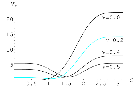
Fig. 1: $V_{\nu}(\theta)$ for $\nu=0.2,~{}0.4$, and $0.5$. The horizontal line shows a sample line of $V_{\nu}(\theta_{0})={R^{4}h^{2}\over r_{0}^{4}+q}=2.0$. The crossing points between this line and the curve of $V_{\nu}$ represnets $\theta_{0}$.

Before giving explicit solution, we show how the type of solutions is controlled by $h$. From the definition of $h$ given in Eq. (15), we obtain

$${p_{\theta}^{2}\over r^{2}}+p_{r}^{2}=\left({R\over r}\right)^{4}\left({r^{4}+q\over R^{4}}V_{\nu}-h^{2}\right)$$ (22)

then from the reality of the solution, the next constraint is obtained

$${r^{4}+q\over R^{4}}V_{\nu}\geq h^{2}~{}.$$ (23)

At the end points, $x=x_{\pm}$, $\theta=\pi$ and $r$ could become large, however $r$ takes its minimum $r\simeq r_{0}$ at the mid point $x=0$. Expressing as $\theta|_{x=0}=\theta_{0}$ at this point, the value of $\theta_{0}$ is obtained by solving the equation,

$${r_{0}^{4}+q\over R^{4}}V_{\nu,\theta_{0}}=h^{2}~{}.$$ (24)

This equation has two solutions for $\theta_{0}$ when $h$ is large as shown in the Fig. 1, but there is one or no solution for small $h$. The solutions of the former (latter) case of large (small) $h$ are identified with the baryonium (baryon).

Consider the baryonium solution. From (24), $r_{0}$ is given as

$$r_{0}=\left({R^{4}h^{2}\over V_{\nu}(\theta_{0})}-q\right)^{1/4}\,.$$ (25)

While the exact solutions are obtained by solving the above four Hamiton equations (20) and (21) as given below, we show an approximate solution in the region where we can assume $\dot{r}\sim 0$ and $r\sim r_{0}$ near $x=0$. Under this assumption, we obtain from (22)

$$\dot{\theta}=\pm{r_{0}\over R^{4}h}\sqrt{r_{0}^{4}+q}\sqrt{V_{\nu}(\theta)-V_{\nu}(\theta_{0})}$$ (26)

then we solve this as

$$x(\theta)=\pm\int_{\theta_{0}}^{\theta}d\theta~{}{R^{4}h\over r_{0}\sqrt{r_{0}^{4}+q}\sqrt{V_{\nu}(\theta)-V_{\nu}(\theta_{0})}}$$ (27)

This solution is symmetric with respect to $x=0$ axis in $x$-$\theta$ plane. The important point of this approximate solution is that the solution runs from $x=0$ to two opposite directions, however they are going to the same pole on $S^{5}$ but with different values of $x$. In order to see the behavior of the solution far from $\theta_{0}$, we must solve the exact form of equations. Actually we can find the solutions as stated above exactly, namely they satisfy this symmetry at all $\theta$ even if the assumption imposed here is not satisfied.

Which pole, $\theta=0$ or $\pi$, is chosen depends on the value of $\theta_{0}$. Notice that $V_{\nu}(\theta)$ has a minimum at $\theta_{c}$ which is given as a slolution of

$$\pi\nu=\theta_{c}-\sin\theta_{c}\cos\theta_{c}~{}.$$ (28)

and we find the minimum value as $V_{\nu}(\theta_{c})=\sin^{6}(\theta_{c})$. This implies that the pole $\theta=0$ ($\theta=\pi$) is chosen for $\theta_{0}<\theta_{c}$ ($\theta_{0}>\theta_{c}$). This is understood well from the Fig. 1. We notice however that the number of $\theta_{0}$ depends on the value of $h$ as seen for $\nu=0.2$ as seen in the Fig. 1. The situation is however changed by the value of $h$ to find two $\theta_{0}$ also for $\nu=0.2$.

But for the case of $\nu=0$, there is only one $\theta_{0}$ for any value of $h$. In this case, the baryonium is constructed by $N$-quarks and anti-$N$-quarks attached at each end points. In other words, we obtain a bound state of baryon and anti-baryon without any loss of quark and anti-quark by their pair annihilation.

On the other hand, for the case of $\nu=1/N$, we expect another interesting baryonium configuration which is constructed by one quark and one anti-quark. This state is very similar to the usual mesons, but it is different from them in the point that the D5 vertex is included except for a quark and an anti-quark pair in this state.

Numerical solutions

Here we give the explicit baryonium solutions mentioned above. The equations are solved numerically since it would be impossible to solve them analytically. Firstly, we give a way to obtain the symmetric solutions. It is convenient to set the following boundary conditions at $x=0$ as

$$\theta(0)=\theta_{0}\,,\quad r(0)=r_{0}\,,\quad{\rm and}~{}~{}p_{r}(0)=p_{\theta}(0)=0$$ (29)

They are given as follows. First, an appropriate $\theta_{0}$ is given for fixed $h$, then $r_{0}$ is determined by the above relation (25). The last two conditions, $p_{r}(0)=p_{\theta}(0)=0$, are necessary to obtain a baryonium solution which is symmetric with respect to $x=0$ axis.

Fig. 2: The typical $D5/\overline{D5}$ solution for $q=0.3$, $\nu=0.5$ at $h=-1$ and $\theta_{0}=1.6708$. The boundary conditions are $p_{r}(0)=p_{\theta}(0)=0$.

Fig. 3: The 3d graphic of $D5/\overline{D5}$ solution given in the Fig. 2 for $q=0.3$, $\nu=0.5$ at $h=-1$ and $\theta_{0}=1.6708$.

An explicit example of the baryonium solution is obtained for $\nu=0.5$, $h=-1$ and $\theta_{0}=1.6708$ under the above boundary conditions (29). The results are shown in the Figs. 2 and 3. From the Fig. 2, we can easily understand the fact that this solution is interpreted as the $D5/\overline{D5}$ bound state solution. This kind of solutions can be obtained at any $\nu$, and it can be considered as the vertex part of a baryonium of $(1-\nu)N$ quarks and $(1-\nu)N$ ant-quarks which are attached at each end point of the vertex for general $\nu$.

Here, in the Fig. 4, we show the $\nu=0.7$ case as an example.

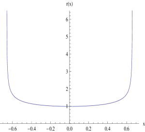
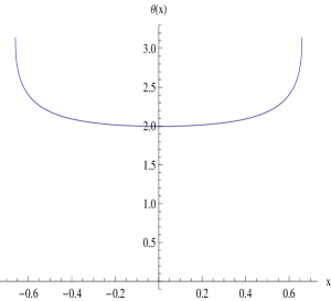
Fig. 4: $D5/\bar{D5}$ solution for $q=0.3$, $\nu=0.7$ at $h=-1$ and $\theta_{0}=1.9962$. The boundary conditions are $p_{r}(0)=p_{\theta}(0)=0$.

Asymmetric solution

While the symmetric solutions are examined above, the various asymmetric solutions are also obtained when we solve the same equations with a slightly different boundary conditions from the one of the symmetric solutions. For example, they are obtained by changing the boundary conditions, (29). These solutions are also regarded as the baryonium since they connect two cusps in the same side, at $\theta=\pi$ (or at 0) at different $x$.

An example of a little asymmetric solution is shown in the Fig. 5, where boundary conditions are changed to $p_{r}(0)=0$ and $p_{\theta}(0)=10^{-4}$.

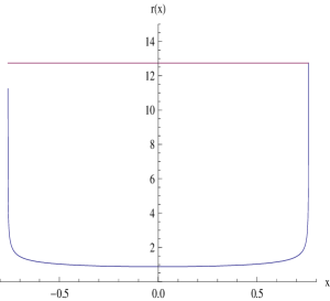
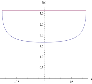
Fig. 5: The typical $D5/\overline{D5}$ solution for $q=0.3$, $\nu=0.5$ at $h=-1$ and $\theta_{0}=1.6708$. The boundary conditions are $p_{r}(0)=0$, $p_{\theta}(0)=10^{-4}$.

In general, the energy of the asymmetric solution becomes higher than the symmetric one. In this sense, the stable configurations can be considered as the maximally symmetric one. Then, we consider hereafter symmetric solutions.

Another kind of solution obtained by a different boundary conditions is the one called as the split baryon, which represents a baryon vertex. We give comments to this solution in the next section.

Stability of the baryonium vertex

In the next, we study the stability of the baryonium solution obtained above. From the viewpoint of energy, we concentrate on the symmetric vertex solutions, which are discriminated by its length $L$. Here $L$ is defined as

$$L\equiv x_{+}(\pi)-x_{-}(\pi)\,,$$ (30)

where we assume $x_{+}(\pi)>x_{-}(\pi)$. Depending on the boundary value $\theta_{0}$, both the $L$ and the vertex energy $U$, which is given by (14), vary. So, by varying $\theta_{0}$ for fixed $h$, the relation between $U$ and $L$ is examined for the symmetric solutions. This relation could give us a critical check for the stability of the baryonium configuration.

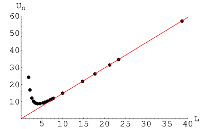
Fig. 6: The left: The normalized vetex energy $U_{n}=U/({N\over 3\pi^{2}\alpha^{\prime}})$ versus its length in the x-direction for $D5/\overline{D5}$ solution for $\nu=0.5$, $q=0.3$, $R=1$ and $h=-1$. The line represents $U_{n}=1.48L$. The right: The equi-potential curves in ($-h$,$L$) plane. The point A denotes the bottom of the potential.

The numerical results of $U$ and $L$ for $h=-1$ and $\nu=0.5$ are shown in the left hand side of Fig. 6, where the normalized energy density, $U_{n}=U/({N\over 3\pi^{2}\alpha^{\prime}})$, is shown instead of $U$. From this we can see that a clear minimum is found at definite and finite value of $L$. Namely, the state for large $L$ and also for small $L$ needs large energy to form it. Especially, the latter fact means that the baryonium vertex does not vanish to $L=0$. For other values of $h$, similar $U$-$L$ relations are expected and this is assured as follows.

Here, $U$ depends on the two parameters $h$ (or $r_{0}$) and $\theta_{0}$ except for the external parameters $R$ and $q$. Then we can write as $U=U(h,r_{0})$ or $U=U(h,\theta_{0})$. Meanwhile it is possible to replace one of the parameters by a physical quantity, for example $L$, as $U=U(h,L)$.

In order to assure the minimum of $U$ in the two dimensional parameter space, we show the equi-potential curves (contour for $U$) in the $h$-$L$ plane. The numerical results are shown in the right hand side of the Fig. 6. From this, we find a minimum does exist near the point A, and we find that the minimum given in the left figure is near the same $L$ of point A. In general, we can consider many kinds of paths in this plane to study similar $U$-$L$ relation along it.

From the above results, we could read the following points.

(i) The energy density $U$ has a minimum at a finite $L$. This implies the stability of the baryonium configuration against the tachyon, which would appear as strings connecting between D5 and anti-D5 branes. The mass square of this string is given as $L^{2}/R^{4}-1/(2\pi\alpha^{\prime})$ [24], then it is stable for enough large $L$. Here the size of $L$ is measured by the scale $R$, the AdS₅ radius, so we can set the parameters to satisfy the inequality,

$$L^{2}/R^{4}>{1\over 2\pi\alpha^{\prime}}\,,$$ (31)

at least around the $L$ where $U$ is minimum.

(ii) Secondly, at large $L$, $U$ increase linearly with respect to $L$, and we can approximate its behavior as

$$U=\tau_{B}L\,.$$ (32)

where $\tau_{B}$ denotes the tension of the baryonium vertex. The value in the case given in the Fig. 6 is evaluated and shown by a line. However, we must notice that the above result is obtained for $h=-1$ and $\tau_{B}$ depends on $h$ as seen from the right hand figure of $U(h,L)$. So we must be careful to study the tension of the baryonium vertex. On this point, we do not discuss furthermore.

4 Baryonium and split baryon

As discussed in [11, 18], the baryon vertex has two types of solutions, that is, the point and split one. The latter is similar to baryonium vertex in the sense that it has a finite length in our space.

As mentioned above, the baryon vertex configurations are also obtained by solving the same equations with somewhat different boundary conditions. As given in [18, 19], an easy way to obtain the baryon vertex, which extends also in the $x$-direction with the two end points $x(\pi)$ and $x(0)$, is as follows. First, set the boundary condition at $\theta=\theta_{c}$, where $\theta_{c}$ is the minimum point of $V_{\nu}(\theta)$ as given in (28), as

$$p_{\theta}|_{\theta=\theta_{c}}=\eta\neq 0~{},\quad p_{r}|_{\theta=\theta_{c}}=0~{}.$$ (33)

This boundary condition is necessary to embed the D5 brane on the whole region of $S^{5}$. In other words, the polar angle $\theta$ must cover the whole range $0\leq\theta\leq\pi$, and this becomes possible under the condition $\eta\neq 0$ in (33). This is the important point to identify the obtained configuration with the baryon vertex. Namely, the two end points are at different polar angles, $\theta=0$ and $\theta=\pi$.

For the split baryon vertex obtained in this way, we examine its energy. Roughly speaking, its configuration can be separated to the two parts of extending to $x$ and to $r$ directions. And each part shears the energy of the vertex. We find that the split baryon vertex can be smoothly deformed to the point vertex by suppressing its energy. Then the configuration of minimum energy is realized by the point vertex solution $r=q^{1/4}$ [18, 19]. This point is the important difference from the case of the baryonium, which could not be pushed to a point in spite of the fact that the baryonium is made of $D5/\overline{D5}$.

As for the total mass of the baryon or baryonium, we must add F-strings under the appropriate conditions called as no force condition [18]. In this case, we could find that the minimum energy of split baryon is realized when the length of the F-strings vanishes but the vertex length is finite.

Similar situation is also expected for the case of the baryonium. We examined the energy of baryonium for $\nu=0.5$, $q=0.3$, $R=1$, $r_{\rm max}=10$ and $h=-1$. Then we could find that the minimum of the energy is found when the F-string length vanishes as in the split baryon. However the details of the analyses are not given here. We will give them in the near future.

5 Summary and Discussion

We find a baryonium solution, which can be interpreted as bound state of baryon and anti-baryon, by solving the equations of motion for the D5 brane action. The reason why the bound state $D5/\overline{D5}$ is obtained from the D5 brane action is that the action used to solve the equations contains the displacement flux operator $D$ in the squared form $D^{2}$. This fact enables us to obtain the baryonium configuration, which is made by connecting a D5 brane and its anti-brane, from a D5 brane action which we used.

The configuration of the baryonium vertex looks like a string in our three dimensional space and we find that its size or length $L$. Its energy $U$ depends on the length $L$, and we can show the minimum of $U$ is realized at finite $L$. Then the size is kept finite in its stable state, and we could assure that its configuration in the bulk is in a form that the $D5$ and $\overline{D5}$ are separated enough not to be destabilized by the tachyon. Then we can say that the baryonium state found here would be stable and it would be difficult to observe its decay into mesons. This would be related to the selection rule for hadronic decay and the resultant narrow width of the baryonium[25].

The baryonium vertex solution given here is similar to a baryon vertex configuration which also looks like a string in our three dimensional space. And they both are obtained from the same equations of motion. However, one of the values of the displacement $D$ at the two cusps for the baryonium is different from the baryon. The sum of $D$ at the two cusps is zero for the baryonium, but it is $N$ for the baryon. The energy minimum for the baryon is realized for $L=0$, which looks like a point in our space. Meanwhile, its configuration looks string like in the bulk.

A real baryonium should be made of the vertex and fundamental strings attached at cusps as performed in the case of baryons. Then the mass spectra for the baryonium are examined to compare the spectra given in recent experiments[26]. The tetra-quark meson corresponds to the baryonium of $\nu=1/3$ and $N=3$. We can estimate the mass spectrum of this state. This would be given in the near future.

Appendix A

Here we show another formulation of solving the equations of motion derived from (9) used in [11, 18]. Firstly, rewrite (9) in terms of a general worldvolume parameter $s$ defined by functions $\theta=\theta(s)$, $r=r(s)$, $x=x(s)$ as:

$$U={N\over 3\pi^{2}\alpha^{\prime}}\int ds~{}e^{\Phi/2}\sqrt{r^{2}\dot{\theta}^{2}+\dot{r}^{2}+(r/R)^{4}\dot{x}^{2}}~{}\sqrt{V_{\nu}(\theta)},$$ (34)

where dots denote derivatives with respect to $s$. Then the momenta conjugate to $r$, $\theta$ and $x$ are given as

$$p_{r}=\dot{r}\Delta,\quad p_{\theta}=r^{2}\dot{\theta}\Delta,\quad p_{x}=(r/R)^{4}\dot{x}\Delta,\quad\Delta=e^{\Phi/2}\frac{\sqrt{V_{\nu}(\theta)}}{\sqrt{r^{2}\dot{\theta}^{2}+\dot{r}^{2}+(r/R)^{4}\dot{x}^{2}}}~{}.$$ (35)

Since the Hamiltonian that follows from the action (14) vanishes identically due to reparametrization invariance in $s$. Then we consider the following identity

$$2\tilde{H}=p_{r}^{2}+\frac{p_{\theta}^{2}}{r^{2}}+\frac{R^{4}}{r^{4}}p_{x}^{2}-\left(V_{\nu}(\theta)\right)e^{\Phi}=0~{}.$$ (36)

Regarding this constraint as a new Hamiltonian, we obtain the following canonical equations of motion,

$$\dot{r} = p_{r}~{},~{}~{}\dot{p}_{r}=\frac{2}{r^{5}}p_{x}^{2}R^{4}+\frac{p_{\theta}^{2}}{r^{3}}+{1\over 2}\left(V_{\nu}(\theta)\right)~{}e^{\Phi}\partial_{r}\Phi,$$ (37)

$$\dot{\theta} = \frac{p_{\theta}}{r^{2}}~{},~{}~{}\dot{p}_{\theta}=-6\sin^{4}\theta\left(\pi\nu-\theta+\sin\theta\cos\theta\right)~{}e^{\Phi},$$ (38)

$$\dot{x} = \frac{R^{4}}{r^{4}}p_{x},~{}~{}\dot{p}_{x}=0$$ (39)

The initial conditions should be chosen such that $\tilde{H}=0$. By solving these equations, we could find the same solutions given above.

Appendix B

Here we calculate the tensions at the cusps [18, 19, 27]. In the present model the tension has $r$-component and $x$-component generally. Denoting $r_{1}=r(\pi)$ and $x_{1\pm}=x_{\pm}(\pi)$, where $x_{1-}<0$, and $x_{1+}>0$, the tensions are given by,

$${{\delta U}\over{\delta r_{1}}}={(1-\nu)N\over{2\pi\alpha^{\prime}}}{{e^{\Phi(r_{1})/2}r^{\prime}_{1}}\over{\sqrt{r_{1}^{2}+r_{1}^{\prime 2}+(r_{1}/R)^{4}x_{1\pm}^{\prime 2}}}},\qquad{{\delta U}\over{\delta x_{1\pm}}}={(1-\nu)N\over{2\pi\alpha^{\prime}}}{{e^{\Phi(r_{1})/2}(r_{1}/R)^{4}x^{\prime}_{1\pm}}\over{\sqrt{r_{1}^{2}+r_{1}^{\prime 2}+(r_{1}/R)^{4}x_{1\pm}^{\prime 2}}}}\,.$$ (40)

In the above equation The factor $(1-\nu)$ comes from $|D(\nu,\theta=\pi)|$.

On the other hand, tension of F-string is derived from the following action,

$$U_{F}={1\over{2\pi\alpha^{\prime}}}\int_{x_{1\pm}}^{x_{\rm max}}dx\,e^{\Phi/2}\sqrt{r_{x}^{2}+(r/R)^{4}}\,.$$ (41)

where $r_{x}=\partial_{r}x$. Then the tension of the F-string is obtained as,

$${{\delta U_{F}}\over{\delta r_{1}}}={1\over{2\pi\alpha^{\prime}}}{{e^{\Phi(r_{1})/2}r_{x}^{(1)}}\over{\sqrt{r_{x}^{(1)2}+(r_{1}/R)^{4}}}}\,,$$ (42)

To compare tensions, we take a “vertical limit”, namely, $r^{\prime}_{1}\to\infty$, $r^{(1)}_{x}\to\infty$. Then the following equality holds;

$${{\delta U}\over{\delta r_{1}}}=(1-\nu)N{{\delta U_{F}}\over{\delta r_{1}}}\,.$$ (43)

The tensions in the $x$-direction vanish in the vertical limit. The above equality means the tension of the cusp equals to $(1-\nu)N$ times that of F-string automatically in the vertical limit in the case of $q>0$.

Other case except vertical limit, the following no-force condtion,

$${{\delta U}\over{\delta r_{1}}}=(1-\nu)N{{\delta U_{F}}\over{\delta r_{1}}}\,,\qquad{{\delta U}\over{\delta x_{1\pm}}}=(1-\nu)N{{\delta U_{F}}\over{\delta x_{1\pm}}}\,,$$ (44)

assures the relation between tensions of cusps and F-strings.

References

- [1] J. Maldacena, “The Large Limit of Superconformal Field Theories and Supergravity,” Adv. Theor. Math. Phys. 2 (1998) 231, hep-th/9711200.
- [2] S. S. Gubser, I. R. Klebanov, and A. M. Polyakov, “Gauge Theory Correlators from Noncritical String Theory,” Phys. Lett. B428 (1998) 105, hep-th/9802109.
- [3] E. Witten, “Anti-de Sitter Space and Holography,” Adv. Theor. Math. Phys. 2 (1998) 253, hep-th/9802150.
- [4] E. Witten, “Baryons and Branes in Anti de Sitter Space,” J. High Energy Phys. 07 (1998) 006, hep-th/9805112.
- [5] D. Gross and H. Ooguri, “Aspects of Large Gauge Theory Dynamics as seen by String theory,” Phys. Rev. D58 (1998) 106002, hep-th/9805129.
- [6] Y. Imamura, “Supersymmetries and BPS Configurations on Anti-de Sitter Space,” Nucl. Phys. B537 (1999) 184, hep-th/9807179.
- [7] C. G. Callan, A. Güijosa, and K. Savvidy, “Baryons and String Creation from the Fivebrane Worldvolume Action,” hep-th/9810092.
- [8] J. Gomis, A. Ramallo, J. Simon and P. Townsend, ”Supersymmetric Baryonic Branes”, JHEP 9911 (1999) 019, hep-th/9907022
- [9] C. Callan and J. Maldacena, “Brane Dynamics from the Born-Infeld Action,” Nucl. Phys. B513 (1998) 198, hep-th/9708147.
- [10] G. Gibbons, “Born-Infeld Particles and Dirichlet p-branes”, Nucl. Phys. B514 (1998) 603, hep-th/9709027.
- [11] C. G. Callan, A. Güijosa, K. G. Savvidy and O. Tafjord, “Baryons and flux tubes in confining gauge theories from brane actions,” Nucl. Phys. B 555 (1999) 183 [arXiv:hep-th/9902197].
- [12] Y. Imamura, “On string junctions in supersymmetric gauge theories,” Prog.Theor.Phys.112:1061-1086,2004, hep-th/0410138.
- [13] A. Brandhuber, N. Itzhaki, J. Sonnenschein, and S. Yankielowicz, “Baryons from Supergravity,” J. High Energy Phys. 07 (1998) 020, hep-th/9806158.
- [14] Y. Imamura, “Baryon Mass and Phase Transitions in Large Gauge Theory,” Prog.Theor.Phys.100:1263-1272,1998, hep-th/9806162.
- [15] H. Liu and A. A. Tseytlin, Nucl. Phys. B 553 (1999) 231 [arXiv:hep-th/ 9903091].
- [16] A. Kehagias and K. Sfetsos, Phys. Lett. B 456, 22(1999) [hep-th/9903109].
- [17] K. Ghoroku and M. Yahiro, Phys. Lett. B 604, 235 (2004) [arXiv:hep-th/ 0408040].
- [18] K. Ghoroku, M. Ishihara, “Baryons with D5 Brane Vertex and -quarks states,” Phys. Rev. D 77, 086003 (2008) [arXiv:hep-th/0801.4216].
- [19] K. Ghoroku, M. Ishihara, A. Nakamura and F. Toyoda, “Multi-quark baryon and color screening at finite temperature,” [arXiv:hep-th/0806.0195].
- [20] C. Athanasion, H. Liu and K. Rajagopal, ”Velocity dependence of baryon screening in hot strongly coupled plasma”, [arXiv:hep-th/0806.0195].
- [21] M. Kruczenski, D. Mateos, R. C. Myers and D. J. Winters, JHEP 0405, 041 (2004) [arXiv:hep-th/0311270].
- [22] T. Sakai and J. Sonnenschein, JHEP 0309, 047 (2003) [arXiv:hep-th/0305049].
- [23] T. Sakai and S. Sugimoto, Prog. Theor. Phys. 113, 843 (2005) [arXiv:hep-th/ 0412141].
- [24] A. Sen, APCPT Winter school lecture, 1999, [arXiv:hep-th/ 9904207].
- [25] P.G.O. Freund, F. Waltz and J. Rosner, Nucl. Phys. bf B13,237 (1969)
- [26] The Belle Collabolation, Phys. Rev. Letters 100, 142001 (2008)
- [27] O. Bergman, G. Lifschytz and M. Lippert, “Holographic Nuclear Physics” [arXive:hep-th/0708.0302].