Self-organization of feedforward structure and entrainment in excitatory neural networks with spike-timing-dependent plasticity

Abstract

Spike-timing dependent plasticity (STDP) is an organizing principle of biological neural networks. While synchronous firing of neurons is considered to be an important functional block in the brain, how STDP shapes neural networks possibly toward synchrony is not entirely clear. We examine relations between STDP and synchronous firing in spontaneously firing neural populations. Using coupled heterogeneous phase oscillators placed on initial networks, we show numerically that STDP prunes some synapses and promotes formation of a feedforward network. Eventually a pacemaker, which is the neuron with the fastest inherent frequency in our numerical simulations, emerges at the root of the feedforward network. In each oscillatory cycle, a packet of neural activity is propagated from the pacemaker to downstream neurons along layers of the feedforward network. This event occurs above a clear-cut threshold value of the initial synaptic weight. Below the threshold, neurons are self-organized into separate clusters each of which is a feedforward network.

I Introduction

Synchronous firing of neurons has been widely observed and is considered to be a neural code that adds to firing rates. For example, experimental evidence suggests the relevance of synchronous firing in stimulus encoding Laurent2002 , feature binding Singer1995 ; Engel2001 , and selective attention Engel2001 ; Fries0105 . Collective dynamical states of neurons including synchrony may appear as a result of self-organization based on synaptic plasticity. Modification of synaptic weights (i.e., weights of edges in the network terminology) often occurs in a manner sensitive to relative spike timing of presynaptic and postsynaptic neurons, which is called spike-timing-dependent plasticity (STDP). In the commonly found asymmetric STDP, which we consider in this work, long-term potentiation (LTP) occurs when presynaptic firing precedes postsynaptic firing by tens of milliseconds or less, and long-term depression (LTD) occurs in the opposite case Gerstner96etc . The amount of plasticity is larger when the difference in the presynaptic spike time and the postsynaptic spike time is smaller Gerstner96etc .

The asymmetric STDP reinforces causal pairs of presynaptic and postsynaptic spikes and eliminate other pairs. Based on this property of STDP, how STDP may lead to various forms of synchronous firing has been studied in both experiments and theory. Synchronous firing in the sense of simultaneity of spike timing can be established in recurrent neural networks when the strength of LTP and that of LTD are nearly balanced Karbowski2002 . Large-scale numerical simulations suggest that reproducible spatiotemporal patterns of spike trains self-organize in heterogeneous recurrent neural networks STDP_synchro_set ; Morrison2007 . Self-organization of clusters of synchronously firing neurons that excite each other in a cyclic manner has also been reported Levy01etc ; Cateau2008 .

We previously showed that STDP leads to formation of feedforward networks and entrainment when there is a pacemaker in the initial network Masuda2007 . We considered random networks of coupled oscillators whose synaptic weights change slowly via STDP. We assumed that the oscillators have a common inherent frequency except a single pacemaker whose inherent frequency is larger. By definition, the rhythm of the pacemaker is not affected by those of other oscillators. The network generated via STDP is a feedforward network whose root is the pacemaker. In a final network, a spike packet travels from the pacemaker to the other neurons in a laminar manner. The neurons directly postsynaptic to the pacemaker fire more or less synchronously just after the pacemaker does. These neurons form the first layer. These neurons induce synchronous firing of the neurons directly postsynaptic to them, which define the second layer. In this fashion, a spike packet starting from the pacemaker reaches the most downstream neurons within relatively short time, which resembles the phenomenology of the synfire chain Diesmann99Abeles91 . Compared to the case of frozen synaptic weights, a pacemaker entrains the rest of the network more easily with STDP in the meaning that entrainment occurs with smaller initial synaptic weights.

The previous work does not explain how pacemakers emerge. No matter whether the pacemakers are intrinsic oscillators or network oscillators, they pace rhythms of other elements without being crucially affected by other rhythms. Although some pacemakers may be “robust” oscillators whose rhythms are insensitive to general input, a more natural explanation may be that pacemakers emerge through synaptic plasticity in a neural network in which pacemakers are initially absent. In this case, emergent pacemakers do not have to be robust oscillators; their rhythms can change in response to external input. The emergent network topology makes such neurons pacemakers by eliminating incoming synapses. A neuron would fire with its own rhythm if it is not downstream to any neuron. This scenario is actually the case for two-neuron networks Zhigulin03pre-Nowotny03jns ; Masuda2007 . Here we are concerned to networks of more than two neurons. An associated question is which oscillator may become a pacemaker.

In this work, we numerically investigate recurrent networks of coupled phase oscillators subject to STDP. We show that, when the initial synaptic weights are strong enough, STDP indeed yields feedforward networks so that downstream neurons are entrained by an emergent pacemaker. To our numerical evidence, the emergent pacemaker is always the neuron with the largest intrinsic frequency. Below the threshold for entrainment, STDP leads to the segregation of the initial neural network into subnetworks of feedforward networks.

II Model

II.1 Coupled phase oscillators

We model dynamics of neural networks by $N$ coupled phase oscillators whose synaptic weights are plastic. Although a majority of real neurons fire in the excitable (i.e., fluctuation-driven) regime, for tractability we use phase oscillators, which fire in an oscillatory manner. Generally speaking, phase transitions are more easily and clearly determined in the oscillatory regime than in the excitable regime. This is a reason why collective neural dynamics phase-osc ; higher including ones associated with STDP Karbowski2002 ; Seliger02 ; Masuda2007 have been analyzed in the oscillatory regime actually to give insights into dynamics of neural networks possibly operating in the excitable regime. In the following, we report numerical results for $N=3$ and $N=100$.

The state of neuron $i$ $(1\leq i\leq N)$ is represented by a phase variable $\phi_{i}\in[0,2\pi)$. We identify $\phi_{i}=0$ and $\phi_{i}=2\pi$. When $\phi_{i}$ crosses $0$ in the positive direction, neuron $i$ is defined to fire. We denote by $t_{j}$ and $t_{i}$ the spike time of presynaptic and postsynaptic neurons. If $\phi_{i}$ crosses 0 in the positive direction as time advances from $t$ to $t+\Delta t$, we set $t_{i}=t+[2\pi-\phi_{i}(t)]/[2\pi+\phi_{i}(t+\Delta t)-\phi_{i}(t)]\Delta t$. As the initial condition, we set $\phi_{i}=0$ $(1\leq i\leq N)$ for $N=3$. We adopt this artificial initial condition to draw phase diagrams to systematically understand possible routes to synchrony via STDP. For $N=100$, $\phi_{i}(0)$ is picked randomly and independently for each $i$ from the uniform density on $[0,2\pi)$. Neuron $i$ is endowed with inherent frequency $\omega_{i}$ so that it fires regularly at rate $\omega_{i}/2\pi$ when isolated. Connectivity between neurons is unidirectional and weighted, consistent with the properties of chemical synapses. The set of edges in a network is denoted by $E$. In other words, $(j,i)\in E$ if neuron $j$ is presynaptic to neuron $i$. Dynamics of the coupled phase oscillators are given by

$$\frac{\mathrm{d}\phi_{i}}{\mathrm{d}t}=\omega_{i}+\frac{1}{\langle k\rangle}\sum_{j:(j,i)\in E}g_{ji}\sin(\phi_{j}-\phi_{i})+\sigma\xi_{i},$$ (1)

where $\langle k\rangle$ is the average in-degree of neuron $i$, $g_{ji}$ is a synaptic weight, and $\xi_{i}$ represents the standard Gaussian white noise independent for different $i$. As a result of the phase reduction theory Kuramotobook , the coupling term in the oscillatory regime is generally given by a $2\pi$-periodic function of the phase difference $\phi_{j}-\phi_{i}$ under the assumption of weak coupling. This is also the case for pulse coupling, for which averaging an original pulse coupling term over one oscillatory cycle results in a coupling term as a function of $\phi_{j}-\phi_{i}$ higher . Modeling realistic synaptic coupling needs a coupling term that contains higher harmonics higher . However, our objective in the present paper is not to precisely describe the neural dynamics but to clarify general consequences of STDP under the oscillatory condition. We thus employ the simplest coupling term (i.e sinusoidal coupling).

For $N=3$, we set the amplitude of the noise $\sigma=0.0071$ so that the phase transitions are sharp enough and artificial resonance that is prone to occur when inherent frequencies satisfy $M_{i}\omega_{i}=M_{j}\omega_{j}$ for small integers $M_{i}$ and $M_{j}$ $(1\leq i<j\leq N)$ is avoided. Accordingly, an independent normal variable with mean 0 and standard deviation $\sigma\sqrt{\Delta t}=0.00071$ is added to each neuron every time step $\Delta t=0.01$; we use the Euler-Maruyama integration scheme with unit time $\Delta t$. To determine the phase transitions for $N=100$, we do not apply dynamical noise because, up to our numerical efforts, the numerical results do not significantly suffer from artificial resonance. In some other simulations with $N=100$, we add different amplitudes of dynamical noise to examine the robustness of the results.

II.2 STDP

With STDP, $g_{ji}$ is repeatedly updated depending on spike timing of neuron $j$ and $i$. Specifically, LTP occurs when a postsynaptic neuron fires slightly after a presynaptic neuron does, and LTD occurs in the opposite case Gerstner96etc . We assume that synaptic plasticity operates much more slowly than firing dynamics. We denote by $A^{+}$ and $A^{-}$ the maximum amount of LTP and that of LTD incurred by a single STDP event. Most of previous theoretical work supposes that $A^{-}$ is somewhat, but not too much, larger than $A^{+}$, to avoid explosion in firing rates and to keep neurons firing Karbowski2002 ; STDP_synchro_set ; Morrison2007 ; Levy01etc ; Cateau2008 ; Masuda2007 . Therefore we set $A^{+}/A^{-}=0.9$. How a single spike pair specifically modifies the synaptic weight is under investigation RubinandGutig ; Morrison2007 , and triplets or higher-order combination of presynaptic and postsynaptic spikes rather than a single presynaptic and postsynaptic spike pair may induce STDP FroemkeandPfister . However, we consider the simplest situation in which STDP modifies synaptic weights in an additive manner and the amount of STDP is determined by the relative timing of a presynaptic and postsynaptic spike pair. A single synaptic modification $\Delta g_{ji}$ triggered by a spike pair is represented by

$$\Delta g_{ji}=\begin{cases}A^{+}\exp(-\frac{t_{j}-t_{i}}{\tau})&\text{$t_{j}-t_{i}<0$}\\ -A^{-}\exp(\frac{t_{j}-t_{i}}{\tau})&\text{$t_{j}-t_{i}>0$}\end{cases},$$ (2)

where $\tau$ is the characteristic time scale of the learning window, which is known in experiments to be 10-20 ms Gerstner96etc . Given that inherent frequencies of many pyramidal neurons roughly range between 5 and 20 Hz, $\tau$ is several times smaller than a characteristic average interspike interval. Therefore, following Masuda2007 , we set $\tau=1/6\times 2\pi/\omega$, where $\omega$ is a typical value of spike frequency that is used to determine $\omega_{i}$. Following our previous work Masuda2007 , we set $\omega=8.1$. Because learning is slow compared to neural dynamics, $A^{-}$ must be by far smaller than a typical value of $g$. To satisfy this condition, we set $A^{-}=0.001$ for $N=3$. When $N=100$, average in-degree $\langle k\rangle$ is set equal to 10. This implies that a neuron receives about five to ten times more synapses than when $N=3$. To normalize this factor, we set it $A^{-}=0.0001$ for $N=100$.

We assume that $g_{ji}$ is confined in $[0,g_{max}]$; all the synapses are assumed to be excitatory, because the asymmetric STDP explained in Sec. I has been found mostly in excitatory synapses. Because dynamical noise is assumed not to be large, all the synaptic weights usually develop until $g_{ji}$ almost reaches either $g_{max}$ or 0, until when we run each simulation run. Note that, even if $g_{ji}=0$ is reached, $(j,i)$ still belongs to $E$. The upper limit $g_{max}$ is determined so that a notion of synchronization that we define in Sec. II.3 does not occur when $g_{ji}=g_{max}$, $\forall(j,i)\in E$. Accordingly, we set $g_{max}=7.5$ and $g_{max}=15$ for $N=3$ and $N=100$, respectively.

II.3 Measurement of synchrony

To obtain the threshold for synchrony in Secs. III.1 and III.2.1, we start numerical simulations with the initial condition $g_{ji}=g_{0}$, $\forall(j,i)\in E$. There are various notions of synchrony. We focus on the possibility of frequency synchrony in which neurons fire at the same rate. In the oscillatory regime, frequency synchrony is commonly achieved in two main ways. One is when neurons are connected by sufficiently strong mutual coupling. Then they oscillate at the same rate and with proximate phases. The other is when some neurons entrain others. When upstream neurons, which serve as pacemakers, entrain downstream neurons so that they are synchronized in frequency, synchronous firing in the sense of spike timing may be missing due to synaptic delay. However, neurons located at the same level in the hierarchy relative to the pacemakers tend to have close spike timing Masuda2007 ; Kori04Kori06 . We explore possible emergence of such dynamics when pacemakers are initially absent in networks.

We quantify the degree of frequency synchrony by order parameter $r$ defined by

$$r=\log_{10}\left[\frac{1}{N}\sum_{i}\left({\tilde{\omega}}_{i}-\frac{1}{N}\sum_{i^{\prime}}{\tilde{\omega}}_{i^{\prime}}\right)^{2}\right],$$ (3)

where $\tilde{\omega_{i}}=\mathrm{d}\phi_{i}/\mathrm{d}t$ is the actual instantaneous frequency of neuron $i$ when coupled to other neurons. If all the neurons fire exactly at the same rate, $r$ would become negative infinity. In the actual frequency synchrony, $r$ takes a large negative value mainly because of time discretization. We manually set $r_{c}=-4$ for $N=3$ and $r_{c}=-9$ for $N=100$, so that $r\leq r_{c}$ corresponds to the full frequency synchrony. The value of $r_{c}$ for $N=100$ is smaller than for $N=3$ for two reasons. First, in the numerical simulations determining the degree of frequency synchrony, dynamical noise is present for $N=3$ and absent for $N=100$. Second, we are concerned to the frequency synchrony of all the neurons so that $\sum_{i}(\tilde{\omega}_{i}-1/N\sum_{i^{\prime}}\tilde{\omega}_{i^{\prime}})^{2}$ is small regardless of $N$; we have to normalize the prefactor $1/N$ in Eq. (3).

III Results

III.1 Networks of three neurons

Our goal is to understand dynamics of large neural networks. As a starting point, we examine network evolution and possibility of frequency synchrony using small networks, which will help us understand dynamics of large networks. Two-neuron networks were previously analyzed Masuda2007 . We need at least three neurons to understand competition between different synapses, pruning of synapses, and effects of heterogeneity. Accordingly, we examine dynamics of different three-neuron networks under STDP.

III.1.1 Complete graph

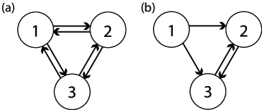
Figure 1: Complete graph (a) without a pacemaker and (b) with a pacemaker.

Consider the complete graph [Fig. 1(a)], in which every pair of neurons is bidirectionally connected. The complete graph does not survive STDP because LTP of a synapse implies LTD of the synapse in the reversed direction and the amount of LTD is assumed to be larger than that of LTP for the same time lag. We examine which synapses survive and whether frequency synchrony emerges through STDP. If a predetermined pacemaker exists in a network, the activity of the other neurons will be entrained into the rhythm of the pacemaker with sufficiently large initial synaptic weights, which was previously shown for $N=2$ and $N=100$ Masuda2007 . Here we consider $N=3$ and compare numerical results when a pacemaker is initially present and absent in the complete graph. Note that the effective initial network when the pacemaker neuron 1 is initially present is the one shown in Fig. 1(b), because the synapses toward the pacemaker are defined to be entirely ineffective.

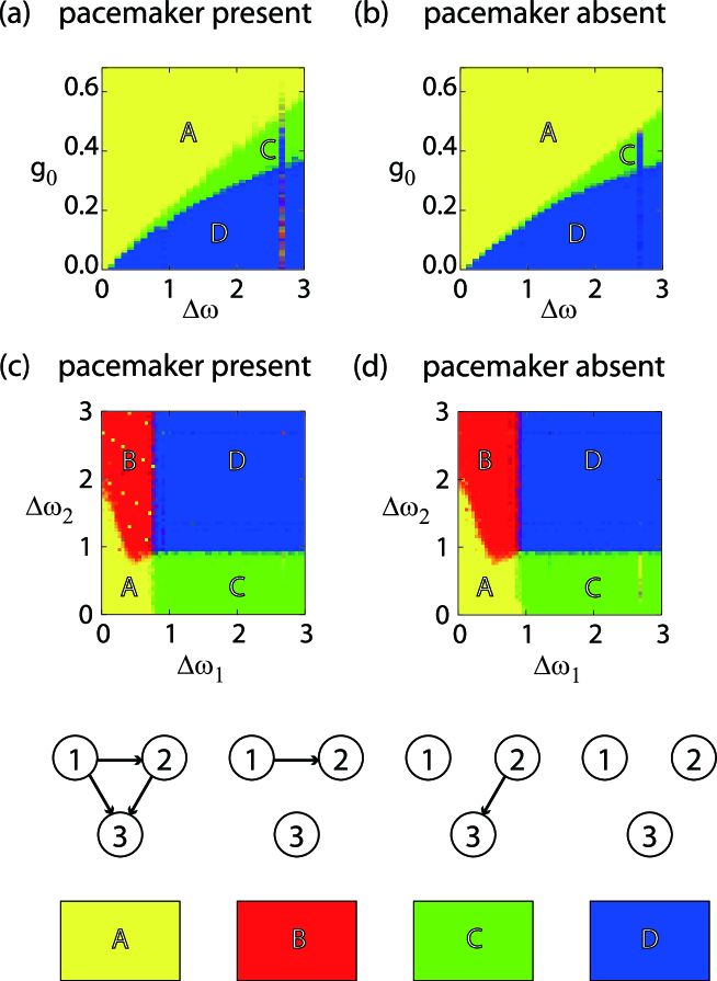
Figure 2: (Color) Phase diagrams for the complete graph in the [(a) and (b)] $\Delta\omega$-$g_{0}$ and [(c) and (d)] $\Delta\omega_{1}$-$\Delta\omega_{2}$ spaces. One pacemaker neuron is initially present [(a) and (c)] or absent [(b) and (d)]. We run numerical simulations 20 times for each pair of parameter values. We add the red element of the RGB color scheme by the maximum amount divided by 20 when $g_{12}$ survives in a simulation run. Similarly, the green is added when $g_{23}$ survives, and the blue is added when all the neurons get disconnected. Yellow regions appear when both $g_{12}$ and $g_{23}$ survive, since the combination of red and green is yellow. In this case, it turns out that $g_{13}$ also survives. We verified that no other connectivity, such as survival of $g_{13}$ without survival of $g_{12}$ or $g_{23}$, and survival of $g_{21}$, $g_{31}$, or $g_{32}$, appears except at points near phase transitions and resonance. Near phase transitions, we exclude such exceptional runs from the statistics. In the resonance regions (e.g., $\Delta\omega\approx 2.7$ and $g_{0}\approx 0.4$), the three neurons may remain connected. In this situation, however, synaptic weights keep oscillating, and any pair of the three neurons is not in frequency synchrony. Therefore, we judge such a run as being completely desynchronized and colored blue (labeled D).

First, we examine the relation between heterogeneity in inherent frequencies, initial synaptic weights, and synchrony. We expect that small heterogeneity and large initial synaptic weights favor synchrony. To focus on phase transitions, we reduce the number of parameters by setting all the initial synaptic weights equal to $g_{0}$ and restrain inherent frequencies $\omega_{1}$, $\omega_{2}$, and $\omega_{3}$ ($\omega_{1}\geq\omega_{2}\geq\omega_{3}$) by imposing, $\omega_{1}-\omega_{2}=\omega_{2}-\omega_{3}\equiv\Delta\omega$, where $\omega_{2}=8.1$. Numerically obtained phase diagrams are shown in Figs. 2(a) and 2(b) for the cases in which a pacemaker is initially present and absent, respectively. The results are qualitatively the same for the two situations. The neurons get disconnected and fire independently as a result of STDP for sufficiently small $g_{0}$ or sufficiently large $\Delta\omega$ (blue regions labeled D). A feedforward network whose root is the fastest oscillator emerges for sufficiently large $g_{0}$ or sufficiently small $\Delta\omega$ (yellow regions labeled A). Then all the neurons rotate at frequency $\omega_{1}$. In the intermediate regime (green regions labeled C), final synaptic weights satisfy $g_{23}\approx g_{max}$ and $g_{12}$, $g_{13}$, $g_{21}$, $g_{31}$, and $g_{32}\approx 0$. In this case, neuron 2 entrains neuron 3 so that they oscillate at frequency $\omega_{2}$, whereas neuron 1 gets disconnected and oscillates at frequency $\omega_{1}$. We rarely observed the case in which neuron 1 entrains 2 (or 3) and neuron 3 (or 2) gets isolated. Although $\omega_{1}-\omega_{2}=\omega_{2}-\omega_{3}$, neuron 1 is more likely to segregate from the network than neuron 3 is. Quantitatively speaking, Figs. 2(a) and 2(b) indicate that the entrainment of the entire network by the fastest neuron (i.e., neuron 1) is to some extent easier to realize when the pacemaker is initially absent than present (yellow regions labeled A). In Figs. 2(a) and 2(b), the phase diagrams are disturbed along vertical lines at $\Delta\omega\approx 2.7$. This artifact comes from the fact that $\omega_{1}$, $\omega_{2}$, and $\omega_{3}$ approximately satisfy the resonance condition (i.e., $M_{1}\omega_{1}=M_{2}\omega_{2}=M_{3}\omega_{3}$ with small integers $M_{1}$, $M_{2}$, and $M_{3}$). In some of the following figures, similar disturbance appears along special lines. We can wash away these artifacts by increasing the amount of dynamical noise. However, we prefer not doing so to prevent the boundaries between different phases from being blurred too much.

Next, to examine what happens when $\omega_{1}$, $\omega_{2}$, and $\omega_{3}$ change independently, we set $g_{0}=0.15$, $\omega_{2}=8.1$, and vary $\Delta\omega_{1}\equiv\omega_{1}-\omega_{2}$ and $\Delta\omega_{2}\equiv\omega_{2}-\omega_{3}$. Numerical results with and without a pacemaker are shown in Figs. 2(c) and 2(d), respectively. Figures 2(c) and 2(d) are similar to each other, except yellow spots in the red region (labeled B) in Fig. 2(c). These spots represent entrainment facilitated due to the artificial resonance condition satisfied by $\omega_{1}$, $\omega_{2}$, and $\omega_{3}$. Both in Figs. 2(c) and 2(d), $g_{23}$ is easier to survive than $g_{12}$ is, consistent with Figs. 2(a) and 2(b). This is indicated by the fact that the phase of the frequency synchrony of the three neurons (yellow regions labeled A) extends to a larger value of $\Delta\omega_{2}>0$ along the line $\Delta\omega_{1}=0$ than to the value of $\Delta\omega_{1}>0$ along the line $\Delta\omega_{2}=0$, and that the phase in which neuron 2 entrains 3 (green, C) survives up to a larger value of $\Delta\omega_{2}$ than the value of $\Delta\omega_{1}$ up to which neuron 1 entrains neuron 2 but not neuron 3 (red, B).

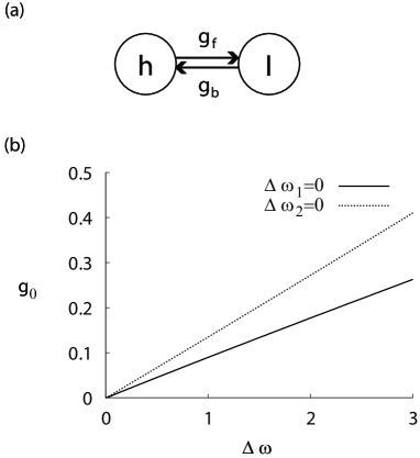
Figure 3: (a) Two-neuron network. (b) Threshold for frequency synchrony for the two-neuron networks corresponding to the $\Delta\omega_{1}=0$ line and the $\Delta\omega_{2}=0$ line in Figs. 2(c) and 2(d).

To examine the cause of the asymmetry in Figs. 2(c) and 2(d) along the two lines $\Delta\omega_{1}=0$ and $\Delta\omega_{2}=0$, we analyze a two-neuron network with asymmetric initial synaptic weights shown in Fig. 3(a). The two neurons $h$ and $l$ have inherent frequency $\omega_{h}$ and $\omega_{l}$ ($\leq\omega_{h}$). The weights of the synapse from neuron $h$ to neuron $l$ and that from neuron $l$ to neuron $h$ are denoted by $g_{f}$ and $g_{b}$, respectively. When $\Delta\omega_{1}=0$ and $\Delta\omega_{2}\geq 0$ in the three-neuron network, neurons 1 and 2 are synchronized almost from the beginning, in both frequency and phase, because $\omega_{1}=\omega_{2}$. This is true if a trivial condition $g_{12}+g_{21}>0$ is satisfied. Then the network is reduced to the two-neuron network by identifying $\omega_{h}=\omega_{1}=\omega_{2}$, $\omega_{l}=\omega_{3}$, $g_{f}=g_{13}+g_{23}$, and $g_{b}=(g_{21}+g_{31})/2$. When, $\Delta\omega_{1}\geq 0$ and $\Delta\omega_{2}=0$ in the three-neuron network, neurons 2 and 3 are synchronized in frequency and phase as far as $g_{23}+g_{32}>0$. Then the network is reduced to the two-neuron network with $\omega_{h}=\omega_{1}$, $\omega_{l}=\omega_{2}=\omega_{3}$, $g_{f}=(g_{12}+g_{13})/2$, and $g_{b}=g_{21}+g_{31}$. For these two situations, we calculate the threshold for frequency synchrony in the two-neuron network using the semi-analytical method developed in Masuda2007 . Because all the synaptic weights are initially equal to $g_{0}$ in Fig. 2, the initial condition for the two-neuron network is $(g_{f},g_{b})=(2g_{0},g_{0})$ for $\Delta\omega_{1}=0$, $\Delta\omega_{2}\equiv\Delta\omega\geq 0$, and $(g_{f},g_{b})=(g_{0},2g_{0})$ for $\Delta\omega_{1}\equiv\Delta\omega\geq 0$, $\Delta\omega_{2}=0$. The phase-transition curves for the frequency synchrony are shown in Fig. 3(b), indicating that the threshold is larger along the $\Delta\omega_{2}=0$ line than along the $\Delta\omega_{1}=0$ line. This is consistent with the three-neuron results shown in Figs. 2(c) and 2(d).

III.1.2 Feedforward loop

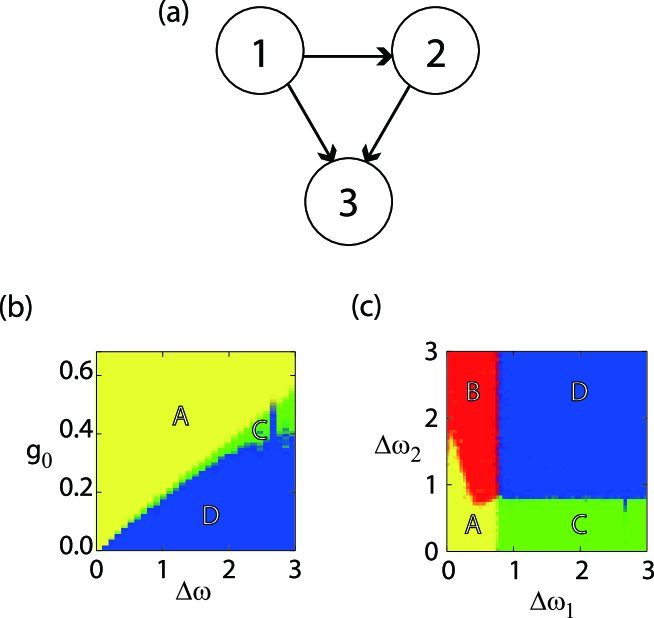
Figure 4: (Color) (a) Feedforward loop. [(b) and (c)] Phase diagrams for the feedforward loop in two different parameter spaces. See Fig. 2 for the color code.

Other three-neuron networks, particularly feedforward ones, are presumably embedded in larger neural networks in the course of network evolution. First, we consider the network shown Fig. 4(a) as the initial network.

Figure 4(a) is the phase diagram in which we vary $\Delta\omega=\omega_{1}-\omega_{2}=\omega_{2}-\omega_{3}$ and $g_{0}=g_{12}=g_{13}=g_{23}$. The original network shown in Fig. 4(a) survives STDP when initial synaptic weights are large or the heterogeneity is small (yellow region labeled A). In the opposite situation, all the neurons get disconnected and fire independently (blue, D). Neuron 1 detaches from the network and neuron 2 entrains neuron 3 in the intermediate regime (green, C).

The phase diagram in the $\Delta\omega_{1}$-$\Delta\omega_{2}$ parameter space with $g_{0}=0.15$ is shown in Fig. 4(b), which looks similar to Figs. 2(c) and 2(d). As in the case of the complete graph, the situation in which neuron 1 entrains neuron 2 with neuron 3 isolated is less likely to arise than that in which neuron 2 entrains neuron 3 with neuron 1 isolated.

III.1.3 Fan-in network

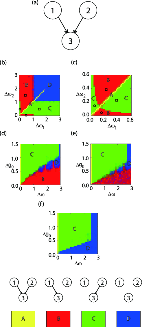
Figure 5: (Color) (a) Fan-in network. [(b) and (c)] Phase diagrams for the fan-in network in the $\Delta\omega_{1}$-$\Delta\omega_{2}$ space, with (c) being an enlargement of (b). We set $g_{0}=0.2$. [(d), (e), and (f)] Phase diagrams in the $\Delta\omega$-$\Delta g_{0}$ space. We set $g_{0}=0.2$, (d) $\omega_{1}=\omega_{3}+0.8$, (e) $\omega_{1}=\omega_{3}+1.0$, and (f) $\omega_{1}=\omega_{3}+1.2$.

Next, we examine dynamics starting from the fan-in network shown in Fig. 5(a). In this network, neuron 3 is postsynaptic to two pacemaker neurons 1 and 2. We are concerned to which neuron entrains neuron 3.

First, we examine the case in which two synapses are initially equally strong and the inherent frequencies of the two upstream neurons are different. Accordingly we set $g_{13}=g_{23}=g_{0}$, $\omega_{1}-\omega_{3}\equiv\Delta\omega_{1}$, $\omega_{2}-\omega_{3}\equiv\Delta\omega_{2}$, $g_{0}=0.2$, and $\omega_{3}=8.1$. Figures 5(b) and 5(c) are the phase diagrams in the $\Delta\omega_{1}$-$\Delta\omega_{2}$ space, with Fig. 5(c) being an enlargement of Fig. 5(b). There are principally four phases: neither neuron 1 or 2 entrains neuron 3 (blue regions labeled D), both neurons 1 and 2 entrain neuron 3 (yellow, A), only neuron 1 entrains neuron 3 (red, B), and only neuron 2 entrains neuron 3 (green, C). The phase diagram is symmetric with respect to the diagonal line $\Delta\omega_{1}=\Delta\omega_{2}$. When $\omega_{1}$ and $\omega_{2}$ are too far from $\omega_{3}$, all the neurons get disconnected (blue, D). Both $g_{13}$ and $g_{23}$ survive only when $\omega_{1}\approx\omega_{2}$ (yellow, A). This phase extends to the disconnection phase (blue, D) on the diagonal because, on this line, the firing of neuron 1 elicits LTP of both synapses so does firing of neuron 2. However, this situation is not generic in that $\omega_{1}$ and $\omega_{2}$ must be very close for this to happen. When $\omega_{1}$ and $\omega_{2}$ are not close to each other and not too far from $\omega_{3}$, which upstream neuron entrains neuron 3 is not obvious. Figure 5(b) tells that a necessary condition for an upstream neuron to entrain neuron 3 is that the difference between its inherent frequency and $\omega_{3}$ is less than $\approx 1.0$. This condition roughly corresponds to the requirement for the entrainment in the two-neuron feedforward network with $g_{0}=0.2$. This explains the two rectangular regions $\Delta\omega_{1}>1.0$, $\Delta\omega_{2}<1.0$, and $\Delta\omega_{1}<1.0$, $\Delta\omega_{2}>1.0$ of Fig. 5(b). In the remaining region (i.e. $\Delta\omega_{1}<1.0$ and $\Delta\omega_{2}<1.0$), the upstream neuron whose inherent frequency is closer to $\omega_{3}$, equivalently, the slower upstream neuron, largely wins the competition (regions marked by $\Box$). The faster upstream neuron entrains neuron 3 when the inherent frequency of the slower upstream neuron is very close to $\omega_{3}$ (regions marked by $\bigcirc$). The total size of the latter regions is much smaller than that of the former regions.

Starting with asymmetric synaptic weights, that is, $g_{13}\neq g_{23}$, the upstream neuron more strongly connected to neuron 3 may entrain neuron 3. To investigate the interplay of this effect and heterogeneity in the inherent frequency, we perform another set of numerical simulations with $\omega_{1}=\omega_{3}+1$, $\omega_{2}=\omega_{1}+\Delta\omega$, $g_{13}=g_{0}$, and $g_{23}=g_{0}+\Delta g_{0}$. The asymmetry in the initial synaptic weight is parameterized by $\Delta g_{0}$. Figures 5(d)-5(f) shows the phase diagrams in the $\Delta\omega$-$\Delta g_{0}$ space for three different values of $\omega_{1}$. On the singular line $\Delta\omega=0$ (i.e., $\omega_{1}=\omega_{2}$), $\Delta g_{0}\geq 0$, both upstream neurons entrain neuron 3. On the line $\Delta\omega\geq 0$ (i.e., $\omega_{1}<\omega_{2}$), $\Delta g_{0}=0$, neuron 1, whose inherent frequency $\omega_{1}$ is closer to $\omega_{3}$ than $\omega_{2}$ is, entrains neuron 3 if $\omega_{1}$ is not too apart from $\omega_{3}$ [Fig. 5(d)]. This is consistent with the results in Figs. 5(b) and 5(c). However, if $g_{23}$ is sufficiently larger than $g_{13}$, neuron 2 overcomes the disadvantageous situation $\omega_{2}-\omega_{3}>\omega_{1}-\omega_{3}$ to win against neuron 1 and entrains neuron 3. We confirmed that neuron 2 exclusively entrains neuron 3 when $\Delta\omega<0$ and $\Delta g_{0}>0$ (not shown).

III.2 Networks of many neurons

In this section, we use networks of heterogeneous $N=100$ neurons to examine what network structure and dynamics self-organize via STDP when we start from random neural networks. The inherent frequencies of the neurons are independently picked from the truncated Gaussian distribution with mean 8.1, standard deviation 0.5, and support $\omega_{i}\in[7.6,8.6]$. We assume that every neuron has $\langle k\rangle=10$ randomly selected presynaptic neurons on average so that an arbitrary pair of neurons is connected by a directed edge with probability $\langle k\rangle/(N-1)\approx 0.1$. Except in Sec. III.2.3, where we investigate effects of heterogeneity, the initial synaptic weight is assumed to be $g_{0}$ common for all the synapses. We vary $g_{0}$ as a control parameter.

III.2.1 Threshold for frequency synchrony

We compare how STDP affects the possibility of entrainment and formation of feedforward networks when a pacemaker is present and when absent. To this end, we fix a random network and a realization of $\omega_{i}$ ($1\leq i\leq N$). Without loss of generality, we assume $\omega_{1}\geq\omega_{2}\geq\cdots\geq\omega_{N}$. For the network with a pacemaker, we make the fastest neuron a pacemaker. By definition, the rhythm of the pacemaker is not affected by those of the other neurons even though the pacemaker is postsynaptic to approximately $\langle k\rangle$ neurons. Using the bisection method, we determine the threshold value of $g_{0}$ above which all the neurons will synchronize in frequency.

The results without dynamical noise (i.e., $\sigma=0$) are summarized in Table I. When the pacemaker is present from the beginning, STDP drastically reduces the threshold for entrainment Masuda2007 . After entrainment, all the neurons rotate at the inherent frequency of the pacemaker, that is, $\omega_{1}=8.60$. When a pacemaker is initially absent, STDP reduces the threshold for frequency synchrony by $34\%$. Facilitation of frequency synchrony in the absence of the initial pacemaker is consistent with the results for the complete graph with $N=3$ (Fig. 2). In this situation, the scenario to frequency synchrony is different between the presence and the absence of STDP. With STDP, the fastest oscillator eventually entrains the entire network when the initial synaptic weight is above the threshold, as in the case of the network with a prescribed pacemaker. Without STDP, the fastest oscillator does not entrain the other neurons. The realized mean frequency 8.08 is close to the mean inherent frequency of the 100 neurons. This suggests that frequency synchrony in this case is achieved by mutual interaction, rather than by one-way interaction underlying the entrainment by the fastest neuron. Therefore, in networks without predetermined pacemakers, STDP enables emergence of pacemakers and changes the collective dynamics drastically.

Table 1: Comparison of the threshold for frequency synchrony $g_{c}$ and the actual mean frequency of the neurons $\left<\tilde{\omega}\right>$ in the frequency synchrony. We calculated $\left<\tilde{\omega}\right>$ by averaging the instantaneous frequency over all the neurons and over the last ten unit times of the simulation.

		Pacemaker
		Present	Absent
	Present	$g_{c}=9.8$	$g_{c}=0.72$
STDP		$\langle\tilde{\omega}\rangle=8.60$	$\langle\tilde{\omega}\rangle=8.60$
	Absent	$g_{c}=51$	$g_{c}=0.93$
		$\langle\tilde{\omega}\rangle=8.60$	$\langle\tilde{\omega}\rangle=8.08$

III.2.2 Network dynamics

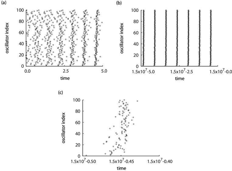
Figure 6: Rastergrams for (a) initial 5 time units and (b) final 5 time units of a simulation run. (c) is an enlargement of (b). We set $N=100$, $g_{0}=1.0$, and $\sigma=0$. The neurons are aligned according to the order of the inherent frequency.

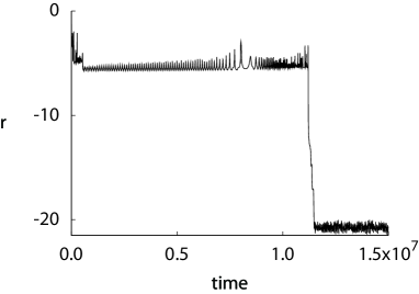
Figure 7: Time course of the degree of synchrony when $N=100$, $g_{0}=1.0$, and $\sigma=0$. The values of $r$ are plotted every 10000 time units.

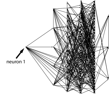
Figure 8: Final network structure when $N=100$, $g_{0}=1.0$, and $\sigma=0$. The network is drawn by Pajek pajek .

For $\sigma=0$, example rastergrams when there is initially no pacemaker and $g_{0}=1.0$, which is above the threshold value 0.72 (see Table I), are shown in Fig. 6. Figures 6(a) and 6(b) correspond to the initial and final stages of a simulation run under STDP, respectively; frequency synchrony appears as a result of STDP. Figure 6(c), which is an enlargement of Fig. 6(b), shows that the fastest neuron entrains the other neurons and that faster neurons tend to fire earlier in a cycle. Figure 7 shows the time course of the degree of synchrony $r$. Around $t=1.2$ x $10^{7}$, $r$ sharply drops, and all the neurons start to oscillate at the same frequency. The effective network defined by the surviving synapses in the final state is drawn in Fig. 8. The neurons are placed so that the horizontal position represents relative spike time in a cycle. With this ordering, the neurons form a feedforward network. In other words, after STDP, if a presynaptic neuron fires later than a postsynaptic neuron in a cycle, this synapse is not present.

Partial entrainment occurs when $g_{0}$ is slightly or moderately smaller than the threshold value 0.72. Circles and crosses in Fig. 9 represent the actual frequency after transient and the inherent frequency of the each neuron, respectively, when $g_{0}=0.5$. The neurons with the same actual frequency belong to the same cluster. Each cluster forms a feedforward network emanating from an emergent pacemaker. Figure 9 indicates that the neurons are divided into two clusters and one isolated neuron. Neuron 2 entrains 85 other neurons all of which are slower than neuron 2, neuron 6 entrains 12 slower neurons, and neuron 1 gets isolated. In this and further numerical simulations we performed, the root of a feedforward subnetwork is always occupied by the fastest neuron in the cluster.

Whether two neurons eventually belong to the same cluster is determined by where these neurons are located on the initial random network and by how close their inherent frequencies are. If $g_{0}$ is smaller than the value used for Fig. 9, two neurons have to be closer in $\omega_{i}$ to stay connected after STDP. Then the number of clusters increases, and the number of neurons in a cluster decreases on average.

III.2.3 Robustness against dynamical noise and heterogeneity

To examine the robustness of the numerical results reported in Sec. III.2.2, we perform additional numerical simulations with dynamical noise and random initial synaptic weights. We draw initial $g_{ji}$ $(j,i)\in E$ randomly and independently from the uniform density on $[0,2g_{0}]$, where $g_{0}=1.0$.

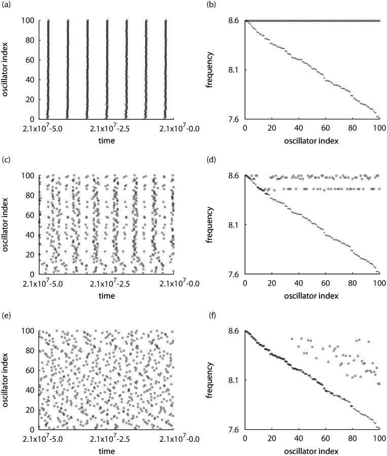
Figure 10: Results for $N=100$, $g_{0}=1.0$, with dynamical noise and heterogeneity in the initial synaptic weights. We set [(a) and (b)] $\sigma=0.081$, [(c) and (d)] $\sigma=0.405$, and [(e) and (f)] $\sigma=0.81$. Rastergrams for 5 time units after transient are shown in (a), (c), and (e). The neurons are aligned according to the order of the inherent frequency. Inherent frequencies ($+$) and actual frequencies ($\circ$) are shown in (b), (d), and (f). Because of the dynamical noise, we estimate the actual frequencies from the phase shifts with bins of width $10^{5}$ time units.

With $\sigma=0.081$, the rastergram and the actual frequency of the neurons after transient are shown in Figs. 10(a) and 10(b), respectively. With $\sigma=0.081$, the standard deviation of the accumulated noise in a unit time, which is equal to $\sigma$, corresponds to 1% of the phase advancement estimated by the mean inherent frequency of the oscillators, which is equal to 8.1. The rastergram [Fig. 10(a)] is indicative of full entrainment. Indeed, all the neurons eventually rotate at the inherent frequency of the fastest neuron [Fig. 10(b)]. With $\sigma=0.405$, the neurons are divided into six synchronous clusters of size 31, 26, 19, 12, 5, 4, plus three isolated neurons [Figs. 10(c) and 10(d)]. With $\sigma=0.81$, many neurons, particularly faster ones, rotate at their inherent frequencies [Figs. 10(e) and 10(f)]. Consequently, there are many clusters of neurons. The frequency synchrony within each cluster is blurred by dynamical noise.

In sum, emergence of entrainment via STDP survives some dynamical noise and heterogeneity in the initial synaptic weights. We have confirmed that, when the entrainment occurs, it is quickly established at around $t=10^{6}$, and the fastest oscillator is located at the root of the feedforward network, as in Fig. 8.

III.2.4 Network motifs

We investigated the evolution of three-neuron networks in Sec. III.1 because we expect that these results have something common with evolution of such subnetworks in large networks. The results in Sec. III.1 predict the following:

• Bidirectional edges do not survive STDP, and feedforward networks of size three will be relatively abundant after STDP. Subnetworks abundant in a large network relative to the case of random networks with the same mean degree (or other order parameters) are called network motifs Milo2002 . The hypothesis that feedforward networks are motifs in large neural networks is consistent with the observations in C. elegans neural networks Milo2002 .

• As a result of STDP, a neuron has at most one effective upstream neuron unless multiple upstream neurons are very close in frequency.

There are 13 connected network patterns of three nodes. How often each pattern appears in a network with $N=100$, relative to the random network, can be quantified by the $Z$ score Milo2002 . The $Z$ score is the normalized number of a pattern in the network, where normalization is given by the mean and the standard deviation of the count of the pattern based on independent samples of the randomized networks. A pattern with a large $Z$ score is a motif of the network with $N=100$.

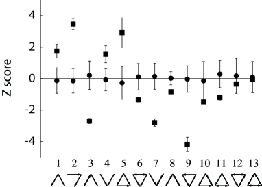
Figure 11: Normalized abundance of different three-neuron network patterns. We set $N=100$, $g_{0}=5.0$, and $\sigma=0$. Circles and squares correspond to the initial and final stages of the simulation runs, respectively.

Figure 11 shows the $Z$ score of each pattern before (circle) and after (square) STDP, calculated by m-finder Alonhp . We set $\sigma=0$ (i.e., no dynamical noise) in this analysis. The error bar shows a range of one standard deviation based on ten simulation runs in each of which we draw a different initial random network and a different realization of $\omega_{i}$ ($1\leq i\leq 100$). Before STDP, the neural network is a directed random graph, so that the $Z$ score for each pattern is around zero, meaning that no pattern is overrepresented or underrepresented significantly. After STDP, the feedforward network whose emergence and survival were observed in Sec. III.1 (i.e., pattern 5 in Fig. 11) and patterns consistent with this (i.e., patterns 1 and 2) are overrepresented. These are motifs of our final networks. Pattern 4 is also a motif in spite of our negation in Sec. III.1 because the two upstream neurons in pattern 4 have the same actual frequency. They are generally different in inherent frequency but share a more upstream ancestor. As the example network in Fig. 8 shows, existence of multiple paths from a neuron to another due to branching and uniting of edges is compatible with STDP. The other network patterns are not significant or underrepresented. These results are further evidence that feedforward networks are formed by STDP in heterogeneous neural networks.

IV Discussion

We have shown using heterogeneous coupled phase oscillators that feedforward networks spontaneously emerge via STDP when the initial synaptic weights are above the threshold value. When this is the case, the pacemaker emerges at the root of the feedforward network and entrains the others to oscillate at the inherent frequency of the pacemaker. Although these results have been known for two-neuron networks Zhigulin03pre-Nowotny03jns ; Masuda2007 , we have shown them for the cases of three and more neurons and quantified the phase transitions separating frequency synchrony and asynchrony. The route to frequency synchrony is distinct from a conventional route to frequency synchrony that occurs when mutual, but not one-way, coupling between oscillators is strong enough. Some results obtained in this work are unique to the networks without a prescribed pacemaker. First, the emergent pacemaker is the fastest oscillator neuron according to our extensive numerical simulations. Note that all the oscillators fire at this frequency in the entrained state, whereas they fire at the mean inherent frequency of the oscillators when the frequency synchrony is realized by strong mutual coupling in the absence of STDP. Second, when the initial coupling strength is subthreshold, the neurons are segregated into clusters of feedforward networks. Third, our numerical evidence suggests that entrainment under STDP occurs more easily when a prescribed pacemaker is absent than present.

In spite of a wealth of evidence that real neural circuits are full of recurrent connectivity DouglasandWilson , feedforward structure may be embedded in recurrent neural networks for reliable transmission of information Diesmann99Abeles91 ; Klemm05 . Feedforward transmission of synchronous volleys in rather homogeneous neural networks as those used in this work serves as a basis of reproducible transmission of more complex spatiotemporal spike patterns in more heterogeneous networks. Such patterns may code external input or appear as a result of neural computation Diesmann99Abeles91 ; STDP_synchro_set . Feedforward structure is also a viable mechanism for traveling waves often found in the brain Ermentrout01neuron . Although computational roles of feedforward network structure are not sufficiently identified, our results give a support to the biological relevance of feedforward networks. The formation of feedforward networks, which we have shown for oscillatory neurons, is consistent with numerical results for more realistic excitable neurons subject to STDP Song01 . The neurons that directly receive external input may be more excited and fire at a higher rate compared to other parts of a neural circuit. Our results suggest that such a neuron or an ensemble of neurons is capable of recruiting other neurons into entrainment and creating feedforward structure.

We assumed the additive STDP with the nearest-neighbor rule in which the dependence of the amount of plasticity on the current synaptic weight and the effects of distant presynaptic and postsynaptic spike pairs, triplets, and so on, are neglected. Generally speaking, evolution of synaptic weights is affected by the implementation of the STDP rule RubinandGutig . However, we believe that our results are robust in the variation of the STDP rule as far as it respects the enhancement of causal relationships between presynaptic and postsynaptic pairs of neurons. Our preliminary numerical data with excitable neuron models suggest that the results are similar between the multiplicative rule RubinandGutig and the additive rule [Kato and Ikeguchi (private communication)]. Recent reports claim the relevance of acausal spike pairs in the presence of synaptic delay Cho2007 ; Cateau2008 . This and other factors, such as different time scales of LTP and LTD Song01 , may let bidirectional synapses survive as observed in in vitro experiments Song2005 . Incorporating these factors is an important future problem.

We have ignored inhibitory neurons for two reasons. First, our main goal is to identify phase transitions regarding synchrony with a simple model. Second, specific rules of STDP are not established for inhibitory neurons, albeit some pioneering results Woodin-Haas . Taking inhibitory neurons into account, preferably in the subthreshold regime, warrants for future work.

Figure 9: Segregation into clusters when $N=100$, $g_{0}=0.5$, and $\sigma=0$. Inherent frequencies ($+$) and actual frequencies after STDP ($\circ$) are shown. We estimate the actual frequencies from the phase shifts with bins of width 10 time units.

- (1) G. Laurent, Nat. Rev. Neurosci. 3, 884 (2002).
- (2) W. Singer and C. M. Gray, Annu. Rev. Neurosci. 18, 555 (1995).
- (3) A. K. Engel, P. Fries, and W. Singer, Nat. Rev. Neurosci. 2, 704 (2001).
- (4) P. Fries, J. H. Reynolds, A. E. Rorie, and R. Desimone, Science 291, 1560 (2001); P. Fries, Trends Cogn. Sci. 9, 474 (2005).
- (5) C. C. Bell, V. Z. Han, Y. Sugawara, and K. Grant, Nature (London) 387, 278 (1997); H. Markram, J. Lübke, M. Frotscher, and B. Sakmann, Science 275, 213 (1997); G. Q. Bi and M. M. Poo, J. Neurosci. 18, 10464 (1998); L. I. Zhang, H. W. Tao, C. E. Holt, W. A. Harris, and M. M. Poo, Nature (London) 395, 37 (1998).
- (6) J. Karbowski and G. B. Ermentrout, Phys. Rev. E 65, 031902 (2002).
- (7) E. M. Izhikevich, J. A. Gally, and G. M. Edelman, Cereb. Cortex 14, 933 (2004); E. M. Izhikevich, Neural Comput. 18, 245 (2006).
- (8) A. Morrison, A. Aertsen, and M. Diesmann, Neural Comput. 19, 1437 (2007).
- (9) D. Horn, N. Levy, I. Meilijson, and E. Ruppin, Adv. Neural Inf. Process. Syst. 12, 129 (2000); N. Levy, D. Horn, I. Meilijson, and E. Ruppin, Neural Netw. 14, 815 (2001); K. Kitano, H. Câteau, and T. Fukai, NeuroReport 13, 795 (2002).
- (10) H. Câteau, K. Kitano, and T. Fukai, Phys. Rev. E 77, 051909 (2008).
- (11) N. Masuda and H. Kori, J. Comput. Neurosci. 22, 327 (2007).
- (12) M. Abeles, Corticonics (Cambridge University Press, Cambridge, 1991); M. Diesmann, M.-O. Gewaltig, and A. Aertsen, Nature (London) 402, 529 (1999); M. C. W. van Rossum, G. G. Turrigiano, and S. B. Nelson, J. Neurosci. 22, 1956 (2002); N. Masuda and K. Aihara, Neural Comput. 15, 103 (2003); A. Kumar, S. Rotter, and A. Aertsen, J. Neurosci. 28, 5268 (2008).
- (13) V. P. Zhigulin, M. I. Rabinovich, R. Huerta, and H. D. I. Abarbanel, Phys. Rev. E 67, 021901 (2003); T. Nowotny, V. P. Zhigulin, A. I. Selverston, H. D. I. Abarbanel, and M. I. Rabinovich, J. Neurosci. 23, 9776 (2003).
- (14) D. Hansel, G. Mato, and C. Meunier, Europhys. Lett. 23, 367 (1993); D. Hansel, G. Mato, and C. Meunier, Neural Comput. 7, 307 (1995); F. C. Hoppensteadt and E. M. Izhikevich, Weakly Connected Neural Networks (Springer-Verlag, New York, 1997); H. Kori, Phys. Rev. E 68, 021919 (2003); E. M. Izhikevich, Dynamical Systems in Neuroscience: The Geometry of Excitability and Bursting (The MIT, Cambridge, 2006).
- (15) C. C. Chow and N. Kopell, Neural Comput. 12, 1643 (2000); H. Y. Jeong and B. Gutkin, Neural Comput. 19, 706 (2007).
- (16) P. Seliger, S. C. Young, and L. S. Tsimring, Phys. Rev. E 65, 041906 (2002).
- (17) Y. Kuramoto, Chemical Oscillations, Waves, and Turbulence (Springer-Verlag, Berlin, 1984).
- (18) J. Rubin, D. D. Lee, and H. Sompolinsky, Phys. Rev. Lett. 86, 364 (2001); A. Kepecs, M. C. W. van Rossum, S. Song, and F. Tegner, Biol. Cybern. 87, 446 (2002); R. Gütig, R. Aharonov, S. Rotter, and H. Sompolinsky, J. Neurosci. 23, 3697 (2003).
- (19) R. C. Froemke and Y. Dan, Nature (London) 416, 433 (2002); J.-P. Pfister and W. Gerstner, J. Neurosci. 26, 9673 (2006).
- (20) H. Kori and A. S. Mikhailov, Phys. Rev. Lett. 93, 254101 (2004); H. Kori and A. S. Mikhailov, Phys. Rev. E 74, 066115 (2006).
- (21) http://vlado.fmf.uni-lj.si/pub/network/pajek/
- (22) R. Milo, S. Shen-Orr, S. Itzkovitz, N. Kashtan, D. Chklovskii, and U. Alon, Science 298, 824 (2002); S. Itzkovitz, R. Milo, N. Kashtan, G. Ziv, and U. Alon, Phys. Rev. E 68, 026127 (2003); R. Milo, S. Itzkovitz, N. Kashtan, R. Levitt, S. Shen-Orr, I. Ayzenshtat, M. Sheffer, and U. Alon, Science 303, 1538 (2004).
- (23) http://www.weizmann.ac.il/mcb/UriAlon/
- (24) R. J. Douglas, C. Koch, M. Mahowald, K. A. C. Martin, and H. H. Suarez, Science 269, 981 (1995); H. R. Wilson, Spikes Decisions and Actions (Oxford University Press, New York, 1999).
- (25) K. Klemm and S. Bornholdt, Proc. Natl. Acad. Sci. U.S.A. 102, 18414 (2005).
- (26) G. B. Ermentrout and D. Kleinfeld, Neuron 29, 33 (2001).
- (27) S. Song and L. F. Abbott, Neuron 32, 339 (2001).
- (28) M. W. Cho and M. Y. Choi, Phys. Rev. Lett. 99, 208102 (2007).
- (29) S. Song, P. J. Sjöström, M. Reigl, S. Nelson, and D. B. Chklovskii, PLoS Biol. 3, 0507 (2005).
- (30) M. A. Woodin, K. Ganguly, and M.-M. Poo, Neuron 39, 807 (2003); J. S. Haas, T. Nowotny, and H. D. I. Abarbanel, J. Neurophysiol. 96, 3305 (2006).