The Marginal Fermi Liquid - An Exact Derivation Based on Dirac’s First Class Constraints Method

Abstract

Dirac’s method for constraints is used for solving the problem of exclusion of double occupancy for Correlated Electrons. The constraints are enforced by the pair operator $Q(\vec{x})=\psi_{\downarrow}(\vec{x})\psi_{\uparrow}(\vec{x})$ which annihilates the ground state $|\Psi^{0}>$. Away from half fillings the operator $Q(\vec{x})$ is replaced by a set of $first$ $class$ Non-Abelian constraints $Q^{(-)}_{\alpha}(\vec{x})$ restricted to negative energies. The propagator for a single hole away from half fillings is determined by modified measure which is a function of the time duration of the hole propagator. As a result: a) The imaginary part of the self energy - is linear in the frequency. At large hole concentrations a Fermi Liquid self energy is obtained. b) For the Superconducting state the constraints generate an asymmetric spectrum excitations between electrons and holes giving rise to an asymmetry tunneling density of states.

Referee Comments: ”‘It is indeed refreshing to see an attempt at a completely novel route to some of these problems. The new approach presented in the manuscript has the potential of stimulating significant further developments by other researchers. I am looking forward for others to follow in the footsteps of the ideas presented in this paper”’

I INTRODUCTION

The central problem in high $T_{c}$ Superconductivity is to treat correctly the effects of strong electron-electron interactions. We consider the zero temperature region away from half fillings in the absence of the magnetic order. The physics in this regime is governed by the absence of double occupied sites. Based on experimental results we know that once the exchange interaction is added it will generate a superconducting ground state.

For a lattice model the effects of interactions are described within a repulsive Hubbard $U$ interaction. Due to the large on-site repulsion the double occupied state are prohibited. This means that we can project out from the electronic spectrum the double occupied states. As a result the anti-commutation rules for the Fermionic operators are modified and calculations become difficult.

A significant simplification takes place in one space dimension where the method of Bosonization shows that for any finite Hubbard U away from half fillings the physics is governed by two Luttinger Liquids (one for charge and the second one for spin). The limit of $U\rightarrow\infty$ can not be considered in a microscopic formulation. This limit can be taken for the renormalized model within the Renormalization Group ($R.G.$) calculations. One obtains a line of Luttinger fixed points.

The wave function has been obtained from the Bethe ansatz Shiba in the limit $U/t\rightarrow\infty$ (where $t$ is the hopping constant). This solution shows that the spin configuration becomes degenerate at $U=\infty$ and the wave function is a $singlet$ ground state for all values of $0<U<\infty$. This means that the degeneracy at $U=\infty$ is removed by any infinitesimal perturbation $t/U$. A formal way for describing the wave function is to say that the ground state is annihilated by the singlet operator $Q(\vec{x})|\Psi^{0}>=0$, $Q(\vec{x})\equiv\mathbf{\psi}_{\uparrow}(\vec{x})\mathbf{\psi}_{\downarrow}(\vec{x})$. The solution of this last equation shows that the wave function can be written as a product of a singlet state with another unknown state.

For two space dimensions we do not have an exact solution as a function of the Hubbard $U$. Therefore we have to consider the projection of double occupancy which forces us to deal with the question of the modified commutators. A direct approach for dealing with the modified commutators is given by the Hubbard $X$ operators. These operators are a mixture of $Bosonic$ and $Fermionic$ excitations. As expected, this leads to a complicated representation which is difficult to handle Zai . The conventional wisdom in higher dimensions is the method of the slave particles Barnes (slave Fermions, or slave Bosons). The slave particles representation replaces the exclusion of double occupancy by two slave fields (one for charge and one for spin). These excitations are coupled by a $U(1)$ gauge field David ; Wiegmann ; Baskaran ; Lee . For space dimensions $d\geq 2$ the gauge field is in the $confined$ phase, causing the slave particles to be strongly coupled. For some special conditions a $deconfined$ phase might be possible FSch ; Fisher . The slave particles representation works in one dimension Sch since the guage field is in the $deconfined$ phase. In this phase, the excitations are described by solitons which carry fractional quantum numbers Nayak . An explicit solution based on the slave-boson method for the Hubbard $U=\infty$ case has been considered in the literature by Sch within a path integral formulation. This formulation has been criticized in Kopp which argued that the $path$ $integral$ $measure$ for the slave particles is incorrect. The price we pay when we work with the slave particles is that the single particle spectrum is described by a pair of $non$ $physical$ $excitations$!

An alternative approach for dealing with the large $U$ repulsion interaction is to use the Gutzwiller projection method used by Gutz ; Muthu . Using this method combined with a variational procedure, the authors Muthu have constructed a variational wave function for the strongly correlated superconductors. It has been pointed out Anderson that the exclusion of double occupancy is responsible for the strong asymmetry between the hole and the electronic excitations observed in the tunneling spectrum for the optimally doped BSCCO.

One of the successful phenomenological theories used to explain a varieties of experiments is the marginal Fermi liquid theory Varma ; VarmAji , yet the relation of this model to the microscopic theory is not clear.

The recent quantum oscillations observed in the Shubnikov de Haas experiment might raise questions about the validity of different approaches and in particular it might test the validity of the projected wave function Doiron ; Julian .

The purpose of the present paper is to introduce a new method for dealing with the problem of exclusion double occupancy. We propose to use Dirac’s theory for $First$ $Class$ $constraints$ Dirac . The solution of the problem will be formulated in the language of Quantum constraints : for a hamiltonian $H$ and a constraint operator $Q(\vec{x})=\mathbf{\psi}_{\uparrow}(\vec{x})\mathbf{\psi}_{\downarrow}(\vec{x})$ one has to find the many body state $|\Psi^{0}>$ which satisfies, $H|\Psi^{0}>=E|\Psi^{0}>$ and is annihilated by the constraint operator $Q(\vec{x})|\Psi^{0}>=0$. Since the constraint should be satisfied at any time the time derivative of the operator $Q(\vec{x})$ requires that the commutator $[Q(\vec{x}),H]$ must vanish. Away from half fillings we restrict the constraints to negative energies (holes excitations) and obtain a set of $first$ $class$ non-Abelian constraints $Q^{(-)}_{\alpha}(\vec{x})$ $\alpha=1,2,3$ which obey $Q^{(-)}_{\alpha}(\vec{x})|\Psi^{0}>=0$. In order to have a canonical theory in the presence of the constraints, we enlarge the Hilbert space by including new anti-commuting fields Teitelboim ; Holten . As a result when a hole is created at a time $t_{i}$ and destroyed at the time $t_{f}$ the evolution in the enlarged space is canonical. The Physical processes occur at times $t_{i}$ and $t_{f}$ in the Physical Hilbert space. The projection into the physical Hilbert space is done by using proper boundary conditions for the anti-commuting fields Teitelboim ; Holten . Due to the non-commutativity of the constraint, the projection will generate a time dependent non-linear measure for the Lagrange multipliers. As a result, the physical evolution operator for the hamiltonian $H$ with constraints is given by, $\hat{U}_{phys}[t_{f},t_{i}]=e^{\frac{-i}{\hbar}(t_{f}-t_{i})H\int\prod_{\alpha=1}^{3}\mathcal{D}\lambda_{\alpha}(T)e^{\frac{-i}{\hbar}}\sum_{\alpha=1}^{3}\int\lambda_{\alpha}(\vec{x})Q^{(-)}_{\alpha}(\vec{x})\,d^{d}x}$

where $\prod_{\alpha=1}^{3}\mathcal{D}\lambda_{\alpha}$ is a $non-linear$ $measure$ which is generated by projection into the Physical Hilbert space for the non-commuting constraints. The effective interaction for the holes sectors depend explicitly on the time interval $T=t_{i}-t_{f}$.

The effective non local action obtained from the temporal projection is investigated with the help of the R.G. method. We find that the single hole excitation has a width which is linear in frequency and the scattering rate obeys $\frac{1}{\tau}\propto\omega F(\frac{\omega}{v_{F}\Lambda})$ in agreement with the infrared data Schlesinger . The linear frequency width is controlled by the holes density. When the hole density increases the region of the linear frequency width shrinks; for large densities it shrinks to zero and therefore a Fermi liquid behavior is obtained. The theory presented in this paper is applicable away not at half fillings for densities $x>x_{c}$ at zero temperature where the magnetic order has been suppressed. Therefore we will not investigate the metal insulator transition. For a finite hole concentration the addition of a finite exchange interaction $j\neq 0$ (in the $t-j$ model) will give rise to a superconducting phase hdavid . An important question will be to understand the effect of exclusion of double occupancy on the superconducting state. We will show that by projecting out double occupancy, an asymmetry of tunneling density of states is observed. Using this theory we will explain the asymmetric tunneling density of states observed by Pan ; Ando .

The content of this paper is as following: In chapter II we present the adaptation of the method of First Class constraints Dirac ; Vilkov ; Batalin ; Teitelboim ; Holten ; Fulp to Condensed Matter Physics. In section III we present the model for correlated electron and show that the ground state can be obtained within the method of quantum constraints. The exclusion of the double occupied states has been investigated in the literature Gutz ; Muthu using the Gutzviller projection method. The solution of the equation $Q(\vec{x})|\Psi^{0}>=0$ is described by the $Jastrow$ representation Gutz ; Muthu . In chapter IV we show that the method of first class allows for additional non-Abelian constraints which give rise to a non-linear integration measure and replaces the delta function constraint used implicitly in refs.Gutz ; Muthu . Using the first class constraint method we compute the ground state for the high $T_{c}$ superconductors. Chapter V is devoted to the computation of the integration measure. In chapter VI we introduce the canonical phase space action for the $t-j$ model. In chapter VII we consider the explicit case where the exchange interaction is zero. In chapter VIII we introduce two Green’s functions: $G$ (the physical one) and $D$ (the parametrical one). Due to the projection into the physical Hilbert space, the action which governs the single hole propagation is time dependent. The physical Green’s function $G$ is computed in terms of a parametric Green’s function $D$. In chapter $IX$ we perform the R.G. calculation for the effective action at the time interval $T=t_{i}-t_{f}$ using the finite size scaling. Chapter $X$ is devoted to the calculation of the parametric Green’s function $D$. In chapter $XI$ we present the calculation for the physical Green’s function $G$. In particular we show that the relaxation rate is linear in frequency. We believe that this explains the experimental results observed for the optical conductivity given in Schlesinger . Finally in chapter $XII$ we consider the effect of the projected Green’s function on the superconductor ground state . We add a $pairing$ interaction and compute the tunneling density of states for a superconductor using the projected Green’s function. We show that the projection (incorporated into the calculation trough the self energy) gives rise to an asymmetric tunneling density of states, in agreement with the experiments Pan ; Ando .

In chapter $XIII$ we present our conclusion. We have included an Appendix where we discuss the effects of the secondary first class constraints generated by the commutators between the hamiltonian and the primary constraints.

II THE METHOD OF QUANTUM CONSTRAINTS

The purpose of this chapter is to present an adaptation of the method of quantum constraints to Condensed Matter Physics.

We have to find the ground state $|\Psi^{0}>$ under the conditions that a set of operators $Q_{\alpha}(\vec{x})$, $\alpha=1,2....n$ are restricted to be zero! In Quantum Mechanics this means that one has to find the state $|\Psi^{0}>$ which is annihilated by the constraints $Q_{\alpha}(\vec{x})|\Psi^{0}>=0$ and is an eigenstate of the hamiltonian $H|\Psi^{0}>=E|\Psi^{0}>$.

There are two types of constraints :

Second Class constraints Dirac are characterized by a non singular matrix $[Q_{\alpha}(\vec{x}),Q_{\alpha^{\prime}}(\vec{x})]$ where the symbol $[,]$ represents the commutator for the Bosonic constraints. The matrix $[Q_{\alpha}(\vec{x}),Q_{\alpha^{\prime}}(\vec{x})]$ can be inverted and therefore has a non vanishing determinant $det[Q_{\alpha}(\vec{x}),Q_{\alpha^{\prime}}(\vec{x})]\neq 0$ for $\alpha,\alpha^{\prime}=1,...m$ and $m=\frac{n}{2}$. Recently we have used this method to compute the persistent currents in coupled rings genus and study mesoscopic vortices in a two dimensional electron gas PMC .

When the determinant of the constraints vanishes we obtain First Class constraints which will be used to solve the problem of exclusion of double occupancy. According to Dirac Dirac one has to identify all the constraints which must be satisfied at any time.

$$\frac{d}{dt}Q_{\alpha}(\vec{x},t)|\Psi^{0}>=0$$ (1)

From the Heisenberg equation of motion we obtain, $\frac{d}{dt}Q_{\alpha}(\vec{x},t)=\frac{1}{i\hbar}[Q_{\alpha}(\vec{x},t),H]$ where the new constraints are given by the difference between the commutator and a linear combination of the existing constraints, $[Q_{\alpha}(\vec{x},t),H]-\sum_{n=1}^{n}T^{\alpha}_{\beta}Q_{\beta}(\vec{x})$$=\sum_{n=1}^{r}t^{\alpha}_{\beta}q_{\beta}(\vec{x})$. In this equation $T^{\alpha}_{\beta}$ and $t^{\alpha}_{\beta}$ stand for a set of matrix elements and $q_{\beta}(\vec{x})$, $\beta=1,2..r$ represent the new (generated) secondary first class constraints. For the remaining part we will represent the two sets $\alpha=1,2..n$ (the primary first class constraints) and $\beta=1,2..r$ (secondary first class constraints) by one set $(Q_{1}(\vec{x},t),Q_{2}(\vec{x},t),...Q_{n}(\vec{x},t),q_{1}(\vec{x}),q_{2}(\vec{x}),...q_{r}(\vec{x}))\Rightarrow Q_{\alpha}(\vec{x},t)$ where $\alpha=1,2..(n+r)$ is the new index for the two sets. For the remaining part we will assume that $Q_{\alpha}(\vec{x},t)$ are $all$ the first class constraints (no new constraints are generated by higher order commutators of the hamiltonian with all the $n+r$ constraints).

Since the commutator of the constraints can be zero, the inverse of the commutator does not exists. As a result, a modification of the commutation rules as is done for Second Class constraints is not possible Dirac .

To overcome this difficulty one introduces $new$ $constraints$ $\Phi_{\beta}(\vec{x},t)$, $\beta=1,2,..(n+r)$,

$$\Phi_{\beta}(\vec{x},t)|\Psi^{0}>=0$$ (2)

In order to obtain a canonical phase space Itz1 with less variables, we have to project out an even number of constraints (the constraints $Q_{\alpha}(\vec{x})$ and their canonical conjugate one $\Phi_{\alpha}(\vec{x},t)$). This is achieved by demanding that the determinant of the commutator in the enlarged Hilbert space (with the additional unknown constraints $\Phi_{\alpha}(\vec{x},t)$) is not zero.

$$Det[Q_{\alpha},\Phi_{\beta}]\neq 0$$ (3)

As a result we obtain an equivalent theory with a fewer $independent$ degrees of freedom Itz1 . Using this conditions we can compute the The Quantum Evolution Operator.

a) The Quantum Evolution Operator for the $unconstrained$ case is given by $\hat{U}[t_{f},t_{i}]=e^{\frac{-i}{\hbar}(t_{f}-t_{i})H}$.

The matrix elements of the evolution operator are computed according to the path integral method for Grassmann anti-commuting functions Itz2 . Using the Grassmann Coherent states one introduces states $|\psi_{\sigma}(\vec{x})>$ ,$<\overline{\psi}_{\sigma}(\vec{x})|$ which obey; $\mathbf{\psi}_{\sigma}(\vec{x})|\psi_{\sigma}(\vec{x})>=\psi_{\sigma}(\vec{x})|\psi_{\sigma}(\vec{x})>$ and $<\overline{\psi}_{\sigma}(\vec{x})|\mathbf{\psi}^{\dagger}_{\sigma}(\vec{x})=<\overline{\psi}_{\sigma}(\vec{x})|\overline{\psi}_{\sigma}(\vec{x})$ where $(\overline{\psi}_{\sigma}(\vec{x}))^{2}=(\psi_{\sigma}(\vec{x}))^{2}=0$.

This allows us to formulate a field theory in the $Schroedinger$ $representation$ where the role of the $coordinate$ is played by $\psi_{\sigma}(\vec{x})$ and the $canonical$ $conjugate$ momentum $\mathbf{\psi}^{\dagger}_{\sigma}(\vec{x})$ is given by $\mathbf{\psi}^{\dagger}_{\sigma}(\vec{x})=\frac{\delta}{\delta\psi_{\sigma}(\vec{x})}$.

The matrix elements of the quantum evolution operator in the Grassmann space are given by $<\overline{\psi},t_{f}|\psi,t_{i}>=<\overline{\psi}|\hat{U}[t_{f},t_{i}]|\psi>\equiv U[\overline{\psi}_{f},t_{f};\psi_{i},t_{i}]$.

Following Itz2 we obtain the path integral representation for the matrix element $U[\overline{\psi}_{f},t_{f};\psi_{i},t_{i}]$:

$$U[\overline{\psi}_{f},t_{f};\psi_{i},t_{i}] = \int D(\overline{\psi}_{\sigma},\psi_{\sigma})e^{(\frac{1}{2}(\overline{\psi}_{f}\psi_{f}+\overline{\psi}_{i}\psi_{i})+i\int_{t_{i}}^{t_{f}}[\frac{1}{2i}(\overline{\psi}_{\sigma}\frac{d\psi_{\sigma}}{\,dt}-\frac{d\overline{\psi}_{\sigma}}{\,dt}\psi_{\sigma})-H(\overline{\psi}_{\sigma},\psi_{\sigma},t)]\,dt)}$$ (4)

b) The Quantum Evolution Operator for the $constrained$ system will be given in terms of evolution matrix elements $U_{phys}[\overline{\psi}_{f},t_{f};\psi_{i},t_{i}]$ in the Grassmann space. Due to the new constraints Faddeev Fad has shown that a $Superdeterminant$ is needed for the integration measure. Such a formalism has been used by Greco .

A simpler method is to represent the physical evolution operator in terms of $only$ the physical constrained $Q_{\alpha}$. The integration with respect to the $unknown$ $\Phi_{\beta}$ constraints will modify the integration measure from $d\lambda_{\alpha}$ to a $non-linear$ integration measure $\mathcal{D}\lambda_{\alpha}(T=t_{i}-t_{f})$. This allows to represent the $physical$ $evolution$ operator in a form which is similar with to the result given by Klauder :

$$\hat{U}_{phys}[t_{f},t_{i}]=e^{\frac{-i}{\hbar}(t_{f}-t_{i})H}\int\prod_{\alpha=1}^{(n+r)}\mathcal{D}\lambda_{\alpha}(T)e^{\frac{-i}{{\hbar}}\sum_{\alpha=1}^{(n+r)}\int\lambda_{\alpha}(\vec{x})Q_{\alpha}(\vec{x})\,d^{d}x}$$ (5)

Eq.(5) emerges from the canonical phase space formalism which we will present in the remaining part of this chapter.

We introduce the Lagrange multipliers, $\lambda^{\alpha}(\vec{x})$, $\alpha=1,2,..(n+r)$ to enforce the exclusion of double occupancy. In addition we seek new constraints which are canonical conjugates to the original ones. The new constraints $\Phi_{\beta}(\vec{x},t)$, $\beta=1,2,..(n+r)$ are introduced with the help of new Lagrange multipliers $\pi_{\alpha}(\vec{x})$ ,$\alpha=1,2,..(n+r)$. The $complete$ Hamiltonian which contains both type of constraints is given by the hamiltonian $H_{T}$:

$$H_{T}=H+\int[\sum_{\alpha=1}^{(n+r)}\lambda^{\alpha}(\vec{x})Q_{\alpha}(\vec{x})+\sum_{\alpha=1}^{(n+r)}\pi_{\alpha}(\vec{x})\Phi^{\alpha}(\vec{x})]\,d^{d}x$$ (6)

It is convenient to replace the constraint $\Phi^{\alpha}(\vec{x})$ by an $equivalent$ constraint $\chi^{\alpha}(\vec{x})$:

$$\Phi^{\alpha}(\vec{x},t)=-\frac{d}{dt}\lambda^{\alpha}(\vec{x},t)+\chi^{\alpha}(\vec{x},t)$$ (7)

As result, the transformed Hamiltonian which contains the time derivative of the Lagrange multiplier $\lambda^{\alpha}(\vec{x})$ will be modified.

Using the results given in equation $(6)$ and $(7)$ we obtain a $new$ formulation of the constraint problem. At this point it is preferable to work with the canonical phase space momentum-coordinate action $S$. $S=\int\,d^{d}x\int\,dtL$ where $L$ is the Lagrangian and $h(\vec{x})$ is the hamiltonian density for the hamiltonian $H$.

$$L=\sum_{\sigma=\uparrow,\downarrow}i\hbar\psi^{\dagger}_{\sigma}(\vec{x},t)\partial_{t}\psi_{\sigma}(\vec{x},t)+\sum_{\alpha=1}^{(n+r)}\pi_{\alpha}(\vec{x},t)\partial_{t}\lambda^{\alpha}(\vec{x},t)-h(\vec{x},t)-\sum_{\alpha=1}^{(n+r)}(\pi_{\alpha}(\vec{x},t)\chi^{\alpha}(\vec{x},t)+\lambda^{\alpha}(\vec{x},t)Q_{\alpha}(\vec{x},t))$$ (8)

The term $\pi_{\alpha}(\vec{x},t)\partial_{t}\lambda^{\alpha}(\vec{x},t)$ allows to identify the canonical conjugate momentum of $\lambda^{\alpha}(\vec{x})$ with $\pi_{\alpha}(\vec{x})$ which obeys the commutation rules, $[\lambda^{\alpha}(\vec{x}),\pi_{\beta}(\vec{y})]=i\hbar\delta_{\alpha,\beta}\delta(\vec{x}-\vec{y})$.

It is important to point out that equation $(8)$ can be understood as a starting point for our theory where the Lagrange multiplier $\lambda^{\alpha}(\vec{x})$ enforces the constraints $Q_{\alpha}(\vec{x})$. The Quantum nature of the Lagrange multipliers is enforced by demanding the existence of a canonical conjugate variable $\pi_{\alpha}(\vec{x})$. Physically the canonical conjugate momentum must be enforced to be zero. This is done by introducing a new Lagrange multiplier $\chi^{\alpha}(\vec{x})$. As a result our theory will have the set of constraint equations:

$\pi_{\alpha}(\vec{x})|\Psi^{0}>=0$ and $Q_{\alpha}(\vec{x})|\Psi^{0}>=0$.

Which will be enforced by the two sets of Lagrange multipliers: $\chi^{\alpha}(\vec{x})$ and $\lambda^{\alpha}(\vec{x})$.

The new Lagrange multipliers $\chi^{\alpha}(\vec{x})$, $\alpha=1,2,..(n+r)$ have not yet been specified. $VILKOVISKY$ Vilkov has proved a theorem which shows that the role of the new Lagrange multipliers $\chi^{\alpha}(\vec{x})$ is equivalent to the gauge fixing in Quantum Electrodynamics. The proof of the theorem Vilkov ; Batalin is based on the followings steps:

1. The action given in eq.$(8)$ can be represented in an $equivalent$ way using new fermionic fields. One introduces a pair of anti-commuting fields for each one of the constraints $\pi_{\alpha}(\vec{x})|\Psi^{0}>=0$ and $Q_{\alpha}(\vec{x})|\Psi^{0}>=0$.

2. The Lagrange multiplier $\chi^{\alpha}(\vec{x})$ plays the role of gauge fixing condition. The replacement of the action in equation $(8)$ with a new action written in terms of the new Fermionic fields show explicitly that the expectation values for any physical observable is invariant under a change of the Lagrange multipliers $\chi^{\alpha}(\vec{x})\rightarrow\chi^{\alpha}(\vec{x})+\delta(\chi^{\alpha}(\vec{x}))$. Therefore the physical results are $independent$ of the particular choice of the fields $\chi^{\alpha}(\vec{x})$.

An exact mapping of the action given in equation $(8)$ to an equivalent action where the constraints are replaced by new Fermionic fields is possible Vilkov ; Batalin ; Holten . As a result one obtains an enlarged Hilbert space of anti-commuting fields.

We consider the case where the constraints $Q_{\alpha}(\vec{x})$ obey the following relations:

$$[Q_{\alpha},Q_{\beta}]=F^{\gamma}_{\alpha,\beta}(Q_{\gamma})$$ (9)

Where $F^{\gamma}_{\alpha,\beta}(Q_{\gamma})$ is a nonlinear function of the constraint $Q_{\gamma}$ such that for $Q_{\gamma}=0$ we have the result $F^{\gamma}_{\alpha,\beta}(Q_{\gamma}=0)=0$ for any $\alpha$, $\beta$ and $\gamma$.

For this case the $VILKOVISKY$ Vilkov theorem allows the exact mapping of the action in eq.$(8)$ to the new action defined in terms of the new anti-commuting fields.

The mapping is done according to the following steps Holten :

a) For each constraint field $Q_{\alpha}(\vec{x})$ one introduces a pair of anti- commuting real fermions $C^{\alpha}(\vec{x})$ and $b_{\alpha}(\vec{x})$

$$[C^{\alpha}(\vec{x}),b_{\beta}(\vec{x^{\prime}})]_{+}=\delta_{\alpha,\beta}\delta(\vec{x}-\vec{x^{\prime}})$$ (10)

Such that $b_{\beta}(\vec{x^{\prime}})$ acts as an annihilation operator.

b) Similarly the canonical momentum constraints $\pi_{\alpha}(\vec{x})$ is replaced by the pair of anti-commuting real fermions $e^{\alpha}(\vec{x})$ and $f_{\alpha}(\vec{x})$.

$$[e^{\alpha}(\vec{x}),f_{\beta}(\vec{x^{\prime}})]_{+}=\delta_{\alpha,\beta}\delta(\vec{x}-\vec{x^{\prime}})$$ (11)

c) The physical Hilbert space is extended to an enlarged Hilbert space. Therefore the many body state $|\Psi^{0}\rangle$ is replaced by a new state $|\Psi>$ which is build from a Fermionic subspace needed to enforce the constraints. The wave function $<\psi_{\sigma}(\vec{x})|\Psi^{0}>$ is replaced by a wave function in the $enlarged$ Hilbert space

$$<\psi_{\sigma}(\vec{x}),C^{\alpha}(\vec{x});\pi_{\alpha}(\vec{x}),e^{\alpha}(\vec{x})|\Psi>$$ (12)

Where $<\psi_{\sigma}(\vec{x}),C^{\alpha}(\vec{x});\pi_{\alpha}(\vec{x}),e^{\alpha}(\vec{x})|$ is the $coherent$ $state$ representation in the enlarged Hilbert space.

d) According to the theorem (see pages 247, 322-324 in Teitelboim ) the physical wave function $<\psi_{\sigma}(\vec{x})|\Psi^{0}>$ is obtained by the projection $<\psi_{\sigma}(\vec{x}),C^{\alpha}(\vec{x})=0;\pi_{\alpha}(\vec{x})=0,e^{\alpha}(\vec{x})=0|\Psi>$.

The physical evolution operator matrix elements $U_{phys}[\overline{\psi}_{f},t_{f};\psi_{i},t_{i}]$ are obtained once we impose the temporal boundary conditions on the auxiliary fields in the $enlarged$ Hilbert space. We use the following $temporal$ boundary conditions:

$$C^{\alpha}(\vec{x},t_{i})=C^{\alpha}(\vec{x},t_{f})=0$$ (13)

$$e^{\alpha}(\vec{x},t_{i})=e^{\alpha}(\vec{x},t_{f})=0$$ (14)

For the momentum $\pi_{\alpha}(\vec{x},t)$ we use the following boundary conditions:

$$\pi_{\alpha}(\vec{x},t_{i})=\pi_{\alpha}(\vec{x},t_{f})=0$$ (15)

e) In the extended Hilbert space the wave function $|\Psi^{0}>$ is replaced by $|\Psi>$.

In the enlarged Hilbert space we replace the constraints $Q_{\alpha}(\vec{x})$ and $\pi_{\alpha}(\vec{x})$ by a new constraint $\Omega$.

The constraint $\Omega$ operator has to obey

$$\Omega(\vec{x})|\Psi>=0$$ (16)

f) In the extended Hilbert space the hamiltonian $H$ is replaced by $H_{c}$. The operator $\Omega$ obeys the extended Heisenberg equation of motion:

$$i\hbar\frac{d}{dt}\Omega|\Psi>=[\Omega,H_{c}]|\Psi>=0$$ (17)

The extended constrained operator $\Omega$ must be NILPOTENT

$$\Omega^{2}=[\Omega,\Omega]_{+}=0$$ (18)

g) In order to satisfy the NILPOTENCY condition the operator $\Omega$ is written as a sum of two parts

$$\Omega=\Omega_{0}+\Omega_{NL}$$ (19)

Where $\Omega_{0}$ is given by

$$\Omega_{0}=\sum_{\alpha=1}^{(n+r)}C^{\alpha}(x)Q_{\alpha}(x)+\sum_{\alpha=1}^{(n+r)}f^{\alpha}(x)\pi_{\alpha}(\vec{x})$$ (20)

Due to the non commutativity of the constraints $[Q_{\alpha},Q_{\beta}]=F^{\gamma}_{\alpha,\beta}(Q_{\gamma})$ the condition $\Omega^{2}=0$ requires that the constraint operator should have a non linear part given by $\Omega_{NL}$. The most general form of the non linear part $\Omega_{NL}$ is given by:

$\Omega_{NL}(\vec{x})=\sum_{\alpha=1}^{(n+r)}C^{\alpha}(\vec{x})[\int\,d^{d}x^{1}\sum_{\alpha_{1}=1}^{(n+r)}\sum_{\beta_{1}=1}^{(n+r)}..\int\,d^{d}x^{(n+r)}\sum_{\alpha_{n=1}}^{(n+r)}\sum_{\beta_{n=1}}^{(n+r)}\frac{i^{(n+r)}}{2(n+r)!}$

$$\cdot C^{\alpha_{1}}(\vec{x}^{1})..C^{\alpha_{(n+r)}}(\vec{x}^{(n+r)})M_{\alpha\alpha_{1}..\alpha_{n+r}}^{\beta_{1}..\beta_{n+r}}b_{\beta_{1}}(\vec{x}^{1})..b_{\beta_{(n+r)}}(\vec{x}^{(n+r)})]$$ (21)

The matrix $M_{\alpha\alpha_{1}..\alpha_{n+r}}^{\beta_{1}..\beta_{n+r}}$ elements are determined by the condition $\Omega^{2}=0$.

h) The hamiltonian $H_{c}$ represents the extention of $H$ for the extended Hilbert space:

$$H_{c}=H+i\int\,d^{d}x\sum_{\alpha=1}^{(n+r)}\sum_{\beta=1}^{(n+r)}C^{\alpha}(\vec{x})h^{\beta}_{\alpha}(\vec{x})b_{\beta}(\vec{x})+...$$ (22)

The parameters $h^{\beta}_{\alpha}(\vec{x})$ are determined by the equation $[H_{c},\Omega]=0$.

k) The condition $\Omega|\Psi>=0$ guarantees that $\Omega O_{phys}|\Psi>=[\Omega,O_{phys}]|\Psi>$. As a result any physical operator $O_{phys}$ is mapped by the operator $\Omega$ to another physical state, therefore we have $[\Omega,O_{phys}]=0$. This implies that if $|\Psi>$ is a physical state, then $\Omega O_{phys}|\Psi>=[\Omega,O_{phys}]|\Psi>=0$.

This condition shows that any modified physical operator $O_{phys}^{\prime}$ which is related to the original physical operator $O_{phys}$ trough the transformation $O_{phys}^{\prime}=O_{phys}+[\Omega,W]_{+}$ has the same matrix elements as the original operator. The symbol $[,]_{+}$ stands for the anti-commutator and $W$ is a new fermionic operator defined in terms of the Lagrange multipliers $\lambda^{\alpha}(\vec{x})$ and $\chi^{\alpha}(\vec{x})$ and the Fermionic fields.

$$W=\int d^{d}x\sum_{\alpha=1}^{(n+r)}[b_{\alpha}(\vec{x})\lambda^{\alpha}(\vec{x})+e_{\alpha}(\vec{x})\chi^{\alpha}(\vec{x})]$$ (23)

The proof that the operator $O_{phys}^{\prime}=O_{phys}+[\Omega,W]_{+}$ and the operator $O_{phys}$ have the same matrix elements in the extended Hilbert space follows from the identity $[\Omega,[\Omega,W]]=[\Omega^{2},W]=0$ (the nilpotency of $\Omega$).

m) This means that the matrix elements of the hamiltonian $H_{effective}$ are the same as for the hamiltonian $H_{c}$.

$$H_{effective}=H_{c}+[\Omega,W]_{+}\equiv H_{c}+\delta^{(+)}_{\Omega}W$$ (24)

This shows that $\delta^{(+)}_{\Omega}$ acts as an $exterior$ $derivative$ Teitelboim , $\delta^{(+)}_{\Omega}A=[\Omega,A]_{+}$ where $A$ is an arbitrary operator.

n) Following the theorem Vilkov we have the freedom to choose any bosonic fields $\chi^{\alpha}$. In particular the path integral is independent on the choice of the unknown Lagrange multiplier $\chi^{\alpha}(\vec{x})$. The path integral is invariant under the transformation $\chi^{\alpha}(\vec{x})\rightarrow(\chi^{\alpha}(\vec{x}))^{\prime}=\chi^{\alpha}(\vec{x})+\delta(\chi^{\alpha}(\vec{x}))$.

As a result of this theorem one can show Teitelboim that the quantum expectation value of any operator $A(t)$ which commutes with the constraint $[A,\Omega]=0$ is independent of the choice $\chi^{\alpha}$!

$$<A(t)>_{\chi^{\alpha}}=<A(t)>_{\chi^{\alpha}+\delta(\chi^{\alpha}(\vec{x}))}$$ (25)

The method presented in this section will be used to solve the problem of exclusion of double occupancy in the next chapters.

III THE $t-J$ MODEL FOR CORRELATED ELECTRONS

In this section we will present the model for the high $T_{c}$ Superconductors. We will show that the ground state can be computed using the method of First Class constraints Dirac .

For the case that the hopping parameter $t$ and the one site repulsion $U$ obey the condition $(t/U)<1$, the double occupation states are projected out and one obtains an effective hamiltonian $H\Rightarrow PH_{0}P+\frac{PH_{0}(1-P)(1-P)H_{0}P}{U}+...$ where $P=1-n_{\uparrow}n_{\downarrow}$ is the projection operator. The effective model is given by:

$$H=-t\sum_{\vec{x},\vec{a}}\sum_{\sigma=\uparrow,\downarrow}\mathbf{\psi}^{\dagger}_{\sigma}(\vec{x})\mathbf{\psi}_{\sigma}(\vec{x}+\vec{a})+h.c.+\delta H\equiv H_{0}+\delta H$$ (26)

where $\vec{x}$ represents the lattice points and $\vec{a}$ runs over to the nearest neighbor sites. This is the $t-J$ model where $H_{0}$ is the hopping hamiltonian which acts on a restricted Hilbert space where double occupancy is excluded, while $\delta H$ represents the exchange hamiltonian controlled by $J\propto\frac{t^{2}}{U}$.

The Many Body ground state is given by $|\Psi^{0}>$. The exclusion of double occupancy on each lattice point $x$ is imposed by the constraint condition which determines the ground state $|\Psi^{0}>$:

$$\mathbf{\psi}_{\uparrow}(\vec{x})\mathbf{\psi}_{\downarrow}(\vec{x})|\Psi^{0}>=0$$ (27)

We define the constraint field $Q(\vec{x})=\mathbf{\psi}_{\uparrow}(\vec{x})\mathbf{\psi}_{\downarrow}(\vec{x})$. To find the ground state $|\Psi^{0}>$ of the hamiltonian $H_{0}+\delta H$ which obeys the constraints we have to satisfy the following equations:

$$H|\Psi^{0}>=E|\Psi^{0}>\hskip 7.22743ptand\hskip 7.22743ptQ(\vec{x})|\Psi^{0}>=0$$ (28)

Once the ground state $|\Psi^{0}>$ is found, the excitations spectrum is obtained by applying the creation operators on this ground state such that no double occupied excited states are created.

It is easy to see that the solution to eq. $(28)$ can be written in the form:

$$|\Psi^{0}>={\Pi}_{\vec{x}}[1-Q^{+}(\vec{x})Q(\vec{x})]\widetilde{|\Psi^{0}>}$$ (29)

Where $\widetilde{|\Psi^{0}>}$ is a state which must be determined! The state $\widetilde{|\Psi^{0}>}$ belongs to the Gutzwiller class Gutz and is often determined by variational methods Muthu . Two possible choices for $\widetilde{|\Psi^{0}>}$ have been considered: the $BCS$ wave function has been used to compute the $RVB$ state and the $Fermi$ $Liquid$ ground state $|F.S>=\prod_{\vec{K}=0}^{\vec{K}_{F}}\psi^{+}_{\uparrow}(\vec{K})\psi^{+}_{\downarrow}(\vec{K})|0>$ has been introduced to compute the $strongly$ $correlated$ $metallic$ $state$.

In the present paper we will not perform a variational calculation, instead we will compute the ground state wave function by determining the additional conditions which the state $|\Psi^{0}>$ has to satisfy. We will show that using the Fermi surface as a the unperturbed ground state we find two additional constraints, the pair creation constraint $Q^{+}(\vec{x})$ and the hole number constraint $Q_{3}(\vec{x})=1-n_{\uparrow}(\vec{x})-n_{\downarrow}(\vec{x})$. The set of the three non-commuting constraints replace the delta function measure (which results from the condition $Q(\vec{x})|\Psi^{0}>=0$ ) by a non-linear integration measure . It is this measure which generates an effective temporal interaction with a time dependent coupling constant.

These results will be derived in the next chapter using the method of first class constraints introduced in chapter $II$.

IV THE APPLICATION OF FIRST CLASS CONSTRAINTS TO THE PROBLEM OF EXCLUSSION OF DOUBLE OCCUPANCY

In this chapter we will apply the general theory for First Class constraints introduced in chapter II to solve the model presented in chapter III. The eigenfunction $|\Psi^{0}>$ must obey $Q(\vec{x})|\Psi^{0}>=0$. We will show that away from half fillings we can use a set of first class constraints defined only for negative energies $Q^{(-)}_{\alpha}(\vec{x})$ where $\alpha=1,2,3$. The commutator $[Q^{(-)}(\vec{x}),H]$ generates secondary constraints $q^{(-)}_{r}(\vec{x})$, $r=1,2,3$ which will be neglected for describing the low energy physics. The justification for this approximation is given in the appendix of this paper where we show that the effective action generated by the secondary constraints are irrelevant according to the R.G. analysis at low energies.

Due to the constraints, the non interacting Fermi energy will be shifted by $\delta{\mu_{F}}$ to a new value. The metallic behavior will be characterized by the vanishing of the renormalized chemical potential shift $[\delta{\mu_{F}}]_{R}=0$ Shankar .

At half fillings we have two additional constraints: $Q^{\dagger}(\vec{x})$ and the hole number operator $Q_{3}(\vec{x})\equiv 1-[\mathbf{\psi}^{\dagger}_{\uparrow}(\vec{x})\mathbf{\psi}_{\uparrow}(\vec{x})+\mathbf{\psi}^{\dagger}_{\downarrow}(\vec{x})\mathbf{\psi}_{\downarrow}(\vec{x})]$. At half fillings the three constraints satisfy: $Q(\vec{x})|\Psi^{0}>=0$, $Q^{\dagger}(\vec{x})|\Psi^{0}>=0$ and $Q_{3}(\vec{x})|\Psi^{0}>=0$. $Away$ $from$ $half$ $fillings$ we have only one first class constraints $Q(\vec{x})$, the other two constraints are neither first class nor second class. This difficulty can be resolved by modifying the constraints. Away from half fillings we will restrict the constraints only to negative energies /holes excitations $Q^{(-)}_{\alpha}(\vec{x})$ where $\alpha=1,2,3$. We introduce the definitions:

$$\mathbf{\psi}_{\sigma}(\vec{x})=\mathbf{\psi}^{(+)}_{\sigma}(\vec{x})+\mathbf{\psi}^{(-)}_{\sigma}(\vec{x});\mathbf{\psi}^{\dagger}_{\sigma}(\vec{x})=\mathbf{\psi}^{\dagger(+)}_{\sigma}(\vec{x})+\mathbf{\psi}^{\dagger(-)}_{\sigma}(\vec{x})$$ (30)

The notation $(+)$ represents the particles excitations for $positive$ energies and $(-)$ describes the holes excitations for $negative$ energies, both measured with respect to the renormalized Fermi energy.

$\mathbf{\psi}^{(+)}_{\sigma}(\vec{x})$ and $\mathbf{\psi}^{\dagger(-)}_{\sigma}(\vec{x})$ act as a destruction operators with respect to the ground state $|\Psi^{0}>$ and obey $\mathbf{\psi}^{(+)}_{\sigma}(\vec{x})|\Psi^{0}>=\mathbf{\psi}^{\dagger(-)}_{\sigma}(\vec{x})|\Psi^{0}>=0$. From Fetter we learn that the field $\mathbf{\psi}^{(-)}_{\sigma}(\vec{x})$ is build from the Fourier momentum components $\vec{K}\leq\vec{K}_{F}$, where $\vec{K}_{F}$ corresponds to the non-interacting Fermi momentum. Similarly $\mathbf{\psi}^{(+)}_{\sigma}(\vec{x})$ is build from the Fourier momentum components $\vec{K}>\vec{K}_{F}$. The effective renormalization of the Fermi surface caused by the constraints is included into the chemical potential shift $\delta{\mu_{F}}$, which will be computed within the R.G. calculations.

The renormalized ground state $|\Psi^{0}>$ has no particles above $\vec{K}_{F}$ and no holes below $\vec{K}_{F}$. (At this step we do not make any assumption about the nature of the discontinuity of the Fermi Surface (the occupation number at $\vec{K}_{F}$).

Acting with the constraint operator $Q(\vec{x})$ on the ground state $|\Psi^{0}>$ we observe:

$$Q(\vec{x})|\Psi^{0}>=(\mathbf{\psi}^{(+)}_{\uparrow}(\vec{x})+\mathbf{\psi}^{(-)}_{\uparrow}(\vec{x}))(\mathbf{\psi}^{(+)}_{\downarrow}(\vec{x})+\mathbf{\psi}^{(-)}_{\downarrow}(\vec{x}))|\Psi^{0}>=\mathbf{\psi}^{(-)}_{\uparrow}(\vec{x}))\mathbf{\psi}^{(-)}_{\downarrow}(\vec{x})|\Psi^{0}>=0$$ (31)

This equation shows that the constraints can be restricted to the holes type excitations $Q^{(-)}(\vec{x})=\mathbf{\psi}^{(-)}_{\uparrow}(\vec{x}))\mathbf{\psi}^{(-)}_{\downarrow}(\vec{x})$. For positive energies the constraint is automatically satisfied, therefore the constraint $Q(\vec{x})$ is restricted to $Q^{(-)}(\vec{x})$.

Using the holes representation, $\mathbf{\psi}^{(-)}_{\sigma}(\vec{x})$ and $\mathbf{\psi}^{\dagger(-)}_{\sigma}(\vec{x})$ we construct the new representations for the constraints:

$$Q^{(-)}(\vec{x}) = \mathbf{\psi}^{(-)}_{\uparrow}(\vec{x})\mathbf{\psi}^{(-)}_{\downarrow}(\vec{x})$$ (32)

$$Q^{\dagger(-)}(\vec{x}) = [\mathbf{\psi}^{(-)}_{\uparrow}(\vec{x})\mathbf{\psi}^{(-)}_{\downarrow}(\vec{x})]^{\dagger}$$ (33)

$$Q_{3}^{(-)}(\vec{x}) = 1-[\mathbf{\psi}^{\dagger(-)}_{\uparrow}(\vec{x})\mathbf{\psi}^{(-)}_{\uparrow}(\vec{x})+\mathbf{\psi}^{\dagger(-)}_{\downarrow}(\vec{x})\mathbf{\psi}^{(-)}_{\downarrow}(\vec{x})]$$ (34)

It is convenient to work with real constraints. We introduce $two$ $real$ $constraints$, $Q^{(-)}_{1}(\vec{x})$ and $Q^{(-)}_{2}(\vec{x})$ using the $constraint$ $Q^{(-)}(\vec{x})$ and $Q^{\dagger(-)}(\vec{x})$.

$$Q^{(-)}_{1}(\vec{x}) = \frac{1}{\sqrt{2}}(Q^{(-)}(\vec{x})+Q^{\dagger(-)}(\vec{x})$$ (35)

$$Q^{(-)}_{2}(\vec{x}) = \frac{1}{\sqrt{2}i}(Q^{(-)}(\vec{x})-Q^{\dagger(-)}(\vec{x}))$$ (36)

In addition to this two real constraints we have the third real constraint $Q^{(-)}_{3}(\vec{x})$ given by equation $(34)$. The set of the hole type constraints $Q^{(-)}_{\alpha}(\vec{x})|\Psi^{0}>$ ,$\alpha=1,2,3$ represent the Non-Abelian First Class constraints for our problem. The commutators of the constraints obey:

$$[Q^{(-)}_{\alpha}(\vec{x}),Q^{(-)}_{\beta}(\vec{x})]=if_{\alpha,\beta}^{\gamma}Q^{(-)}_{\gamma}(\vec{x})$$ (37)

The $Non$-$Abelian$ $First$ $Class$ $constraints$ are characterized by the $structure$ constants $f_{\alpha,\beta}^{\gamma}$, $f_{\alpha,\beta}^{\gamma}=-f_{\beta,\alpha}^{\gamma}=1$ for $\alpha\neq\beta\neq\gamma$ and zero otherwise.

The commutator of the constraints with the hamiltonian $H$ satisfies the equation:

$[Q^{(-)}_{\alpha}(\vec{x}),H]\approx T^{\alpha}_{\beta}(\vec{x})Q^{(-)}_{\beta}(\vec{x})$, where $T^{\alpha}_{\beta}(\vec{x})$ stands for a set of local matrix operators. The symbol $\approx$ means that the derivatives of the constraints operators have been neglected. This approximation can be seen by computing the commutator of the constraint with the kinetic energy:

$[\mathbf{\psi}_{\sigma=\downarrow}(\vec{x})\mathbf{\psi}_{\sigma=\uparrow}(\vec{x}),H_{0}]=t\sum_{\vec{a}}[\mathbf{\psi}_{\sigma=\downarrow}(\vec{x})\mathbf{\psi}_{\sigma=\uparrow}(\vec{x}+\vec{a})+\mathbf{\psi}_{\sigma=\downarrow}((\vec{x}+\vec{a}))\mathbf{\psi}_{\sigma=\uparrow}(\vec{x})]$

The new secondary constraints are obtained by taking the difference of the commutator $\frac{1}{t}[Q(\vec{x}),H_{0}]$ with the primary first class constraints $Q(\vec{x})$:

$q(\vec{x})\equiv\sum_{\vec{a}}[\mathbf{\psi}_{\sigma=\downarrow}(\vec{x})\mathbf{\psi}_{\sigma=\uparrow}(\vec{x}+\vec{a})+\mathbf{\psi}_{\sigma=\downarrow}((\vec{x}+\vec{a}))\mathbf{\psi}_{\sigma=\uparrow}(\vec{x})]-Q(\vec{x})$

$q^{+}(\vec{x})\equiv\sum_{\vec{a}}[\mathbf{\psi}_{\sigma=\downarrow}(\vec{x})\mathbf{\psi}_{\sigma=\uparrow}(\vec{x}+\vec{a})+\mathbf{\psi}_{\sigma=\downarrow}((\vec{x}+\vec{a}))\mathbf{\psi}_{\sigma=\uparrow}(\vec{x})]^{+}-Q^{+}(\vec{x})$

and

$q_{3}(\vec{x})\equiv\sum_{\vec{a}}[\mathbf{\psi}_{\sigma=\downarrow}(\vec{x})\mathbf{\psi}_{\sigma=\downarrow}(\vec{x}+\vec{a})+\mathbf{\psi}_{\sigma=\uparrow}((\vec{x}+\vec{a}))\mathbf{\psi}_{\sigma=\uparrow}(\vec{x})]-[Q_{3}(\vec{x})-1]$

Using the linear transformation given by equations $(35)$ and $(35)$ we obtain the $new$ set of $secondary$ $first$ $class$ $real$ $constraints$: $q^{(-)}_{r}(\vec{x})$, $r=1,2,3$.

The secondary first class constraints modify the Lagrangian $L$ by $\delta L$ :

$\delta L=\sum_{r=1}^{3}\hat{\pi}_{r}(\vec{x},t)\partial_{t}\hat{\lambda}^{r}(\vec{x},t)-\sum_{r=1}^{3}(\hat{\pi}_{r}(\vec{x},t)\hat{\chi}^{r}(\vec{x},t)+\hat{\lambda}^{r}(\vec{x},t)q^{(-)}_{r}(\vec{x},t))$

where $\hat{\lambda}^{r}(\vec{x},t)$ are the Lagrange multipliers which enforce the secondary constraints and $\hat{\pi}_{r}(\vec{x},t)$ are the canonical momentum conjugated to the new Lagrange multipliers $\hat{\lambda}^{r}(\vec{x},t)$. The integration over the new Lagrange multipliers will generate products of $q^{(-)}_{r}(\vec{x})$ pairs. Such operators will induce effective interactions which have the dimensions of the square of the kinetic energy with two time integrations. According to the analysis given in the Appendix the engineering dimensions for such operators is $-1$ and therefore they are strongly irrelevant at low energies ( in comparison to the engineering dimensions $1$ for the effective interaction due to the primary constraints). Therefore we will ignore the Lagrangian induced by the secondary constraints or/and higher order constraints generated by the commutators $[q^{(-)}_{r}(\vec{x}),H_{0}]$, $r=1,2,3$ (such operators contain higher order derivatives in comparison with the constraints $q^{(-)}_{r}(\vec{x})$).

The canonical phase space action for the holes constraints which replaces eq.$(8)$ (without the generated constraints described by $\delta L$) is given by:

$$L=\sum_{\sigma=\uparrow,\downarrow}i\hbar\psi^{\dagger}_{\sigma}(\vec{x},t)\partial_{t}\psi_{\sigma}(\vec{x},t)+\sum_{\alpha=1}^{3}\pi_{\alpha}(\vec{x},t)\partial_{t}\lambda^{\alpha}(\vec{x},t)-h(\vec{x},t)-\sum_{\alpha=1}^{3}(\pi_{\alpha}(\vec{x},t)\chi^{\alpha}(\vec{x},t)+\lambda^{\alpha}(\vec{x},t)Q^{(-)}_{\alpha}(\vec{x},t))$$ (38)

where $\pi_{\alpha}(\vec{x})$ is the canonical momentum conjugate to the Lagrange multiplier $\lambda^{\alpha}(\vec{x})$. This action has two sets of constraints $Q^{(-)}_{\alpha}(\vec{x})|\Psi^{0}>=0$ and $\pi_{\alpha}(\vec{x})|\Psi^{0}>=0$. The Lagrange multipliers are: $\lambda^{\alpha}(\vec{x})$ and the unknown one $\chi^{\alpha}(\vec{x})$. Using the general theory for First Class constraints presented in section II, we will express the action in eq. $(38)$ using new anti-commuting fields. The anti-commuting fields $C^{\alpha}(\vec{x})$ and $b_{\alpha}(\vec{x})$ are used to replace the holes constraints $Q^{(-)}_{\alpha}(\vec{x},t)$ and the anti-commuting fields $e^{\alpha}(\vec{x})$ and $f_{\alpha}(\vec{x})$ replace the momenta constraints $\pi_{\alpha}(\vec{x})$. The unknown Lagrange multiplies $\chi^{\alpha}$ act as gauge fixing conditions.

We replace the state $|\Psi^{0}>$ by the state $|\Psi>$ defined for the extended Hilbert with the extended constraint operator $\Omega$ for the extended Hilbert space (see eq.$(19)$), $\Omega=\Omega_{0}+\Omega_{NL}$ where $\Omega_{NL}$ is chosen such that the condition $\Omega^{2}=0$ is satisfied.

The operator $\Omega_{0}$ (see eq.$(20)$) is given in terms of the $physical$ $constraints$ $Q^{(-)}_{\alpha}(\vec{x})$ and $\pi_{\alpha}(\vec{x})$:

$$\Omega_{0}=\int d^{d}x\left[\sum_{\alpha=1}^{3}C^{\alpha}(\vec{x})Q^{(-)}_{\alpha}(\vec{x})+\sum_{\alpha=1}^{3}f^{\alpha}(\vec{x})\pi_{\alpha}(\vec{x})\right]$$ (39)

The Nonlinear operator $\Omega_{NL}$ (see eq.$(21)$)is obtained using the structure constants given in eq.$(37)$.

$$\Omega_{NL}(\vec{x})=\sum_{\alpha=1}^{3}C^{\alpha}(\vec{x})\left[\int\,d^{d}x^{1}\sum_{\beta=1}^{3}\sum_{\gamma=1}^{3}\frac{-i}{2}C^{\gamma}(\vec{x})f_{\alpha,\beta}^{\gamma}b_{\beta}(\vec{x}^{1})]\right]$$ (40)

According to the theorem Vilkov the path integral is invariant under the change of the Lagrange multipliers $\chi^{\alpha}(\vec{x})$. For the continuation of this article we will choose $\chi^{\alpha}(\vec{x})=0$ and obtain from eq.$(23)$ the Fermionic operator $W$.

$$W=\int d^{d}x\sum_{\alpha=1}^{3}b_{\alpha}(\vec{x})\lambda^{\alpha}(\vec{x})$$ (41)

We compute the anti-commutator $\frac{i}{\hbar}[W,\Omega]_{+}$ and find:

$$\frac{i}{\hbar}[W,\Omega]_{+}=\sum_{\alpha=1}^{3}\lambda^{\alpha}(\vec{x})Q^{(-)}_{\alpha}(\vec{x})+i\hbar\sum_{\alpha=1}^{3}b_{\gamma}(\vec{x})f^{\alpha}(\vec{x})+\sum_{\alpha=1}^{3}\sum_{\beta=1}^{3}\sum_{\gamma=1}^{3}\frac{1}{\hbar}C^{\beta}(\vec{x})\lambda^{\alpha}(\vec{x},t)f_{\alpha,\beta}^{\gamma}b_{\gamma}(\vec{x},t)$$ (42)

This result allows to obtain the effective hamiltonian in the enlarged space:

$H_{effective}=H_{c}+[\Omega,W]_{+}$ where $H_{c}$ is chosen such that $[H_{c},\Omega]=0$.

In this case the difference between $H_{c}$ and $H$ is given by operators which contain higher order derivatives and therefore are irrelevant for low energy Physics.

Using the effective hamiltonian $H_{effective}=H+[\Omega,W]_{+}$ we obtain the action $S$ as a function of the initial and final times $t_{i}$ and $t_{f}$, $T=t_{i}-t_{f}$ .

$$S[t_{i},t_{f}] = \int_{t_{i}}^{t_{f}}\,dt[\sum_{\sigma=\downarrow,\uparrow}(-i\hbar)\psi_{\sigma}^{\dagger}(x,t)\partial_{t}\psi_{\sigma}(x,t)+\sum_{\alpha=1}^{3}\pi_{\alpha}(x,t)\partial_{t}\lambda^{\alpha}(\vec{x},t)+$$ (43)

$$\sum_{\alpha=1}^{3}\partial_{t}C^{\alpha}(\vec{x},t)b_{\alpha}(x,t)+\sum_{\alpha=1}^{3}\partial_{t}e_{\alpha}(\vec{x},t)f^{\alpha}(x,t)-$$

$$[h(\vec{x},t)+\sum_{\alpha=1}^{3}\lambda^{\alpha}(\vec{x},t)Q^{(-)}_{\alpha}(\vec{x},t)+i\hbar\sum_{\alpha=1}^{3}b_{\alpha}(\vec{x},t)f^{\alpha}(\vec{x},t)+$$

$$i\sum_{\alpha=1}^{3}\sum_{\beta=1}^{3}\sum_{\gamma=1}^{3}\frac{1}{\hbar}C^{\beta}(\vec{x})\lambda^{\alpha}(\vec{x},t)f_{\alpha,\beta}^{\gamma}b_{\gamma}(\vec{x},t)]]$$

For commuting constraints, the last term in eq.$(43)$ vanishes (the anti-commuting fields are decoupled). For such a situation the constraints in eq.$(43)$ can be treated by delta function constraints. Once the non-commutativity of the constraints is considered one generate a non-linear measures for the Lagrange multipliers (due to the last term in eq.$(43)$.

The full Non-Abelian action given in equation $(43)$ describes a canonical evolution in an enlarged Hilbert space. The physical observables are obtained only after we project the extended state into the physical Hilbert space. This is achieved by imposing temporal boundary conditions on the non physical anti-commuting coordinates $C^{\alpha}(x,t)$ ,$e_{\alpha}(x,t)$ and the conjugate momenta $\pi_{\alpha}(\vec{x},t)$ ,$\alpha=1,2,3$.

$$C^{\alpha}(x,t_{i})=C^{\alpha}(x,t_{f})=e_{\alpha}(x,t_{i})=e_{\alpha}(x,t_{f})=\pi_{\alpha}(\vec{x},t_{i})=\pi_{\alpha}(\vec{x},t_{f})=0$$ (44)

The projection into the physical space is achieved by the use of initial time $t_{i}$ and final time $t_{f}$ boundary conditions Teitelboim .

$$U_{phys}[\overline{\psi}_{f}(t_{f});\psi_{i}(t_{i})]\equiv U[\overline{\psi}_{f}(t_{f}),\pi_{\alpha}(x,t_{f})=0,C^{\alpha}(x,t_{f})=0,e_{\alpha}(x,t_{i})=0;\psi_{i}(t_{i})]$$ (45)

The physical evolution matrix elements are given by:

$$U_{phys}[\overline{\psi}_{f}(t_{f});\psi_{i}(t_{i})]=\int D(\overline{\psi}_{\sigma},\psi_{\sigma})D(C^{\alpha},b_{\alpha})D(e_{\alpha},f^{\alpha})D(\lambda^{\alpha},\pi_{\alpha})exp[\frac{1}{2}(\overline{\psi}_{f}\psi_{f}+\overline{\psi}_{i}\psi_{i}+\frac{i}{\hbar}S[t_{i},t_{f}]]$$ (46)

Where $S[t_{i},t_{f}]$ is the action in equation $(43)$ . $D(\overline{\psi}_{\sigma},\psi_{\sigma})$ represents the Grassmann measure, $D(C^{\alpha},b_{\alpha})$ and $D(e_{\alpha},f^{\alpha})$ represents the integration measure Teitelboim for the fictitious non-commuting degrees of freedom. $D(\lambda^{\alpha},\pi_{\alpha})$ is the phase space integration over the Lagrange multipliers and the canonical conjugated variables. The action $S[t_{i},t_{f}]$ can be written as a sum of the $physical$ $action$ $\widetilde{S}[t_{i},t_{f}]$ and a $non-physical$ $action$ $S^{ghost}[t_{i},t_{f}]$ given in terms of the non-commuting degrees of freedom $C^{\alpha}$,$b_{\alpha}$ and $e_{\alpha}$ , $f^{\alpha}$:

$$S[t_{i},t_{f}]\equiv\widetilde{S}[t_{i},t_{f}]+S^{ghost}[t_{i},t_{f}]$$ (47)

For fixed values of $t_{i}$ and $t_{f}$ we integrate over the $non-physical$ non-commuting degrees of freedom $C^{\alpha}$,$b_{\alpha}$ and $e_{\alpha}$ , $f^{\alpha}$. We obtain an effective action $S^{eff.}[\lambda^{\alpha};t_{i},t_{f}]$ as a function of the time interval and the Lagrange multipliers. This action is obtained once the non-physical fermions fields have been integrated out and the boundary conditions for the conjugate momenta $\pi_{\alpha}(t_{i})=\pi_{\alpha}(t_{f})=0$ have been used.

$$e^{\frac{i}{\hbar}S^{eff.}[\lambda^{\alpha};t_{i},t_{f}]}\equiv\int\,D(C^{\alpha},b_{\alpha})D(e_{\alpha},f^{\alpha})e^{\frac{i}{\hbar}S^{ghost}[t_{i},t_{f}]}|_{\pi_{\alpha}(t_{i})=\pi_{\alpha}(t_{f})=0}$$ (48)

This allows to represent the matrix elements of the physical evolution operator by the formula:

$$U_{phys}[\overline{\psi}_{f}(t_{f});\psi_{i}(t_{i})] = \int D(\overline{\psi}_{\sigma},{\psi}_{\sigma})D(\lambda^{\alpha})e^{\frac{i}{\hbar}S^{eff.}[\lambda^{\alpha};t_{i},t_{f}]}e^{[\frac{1}{2}(\overline{\psi}_{f}\psi_{f}+\overline{\psi}_{i}\psi_{i})+\frac{i}{\hbar}\widetilde{S}[t_{i},t_{f}]]}=$$ (49)

$$\int D(\overline{\psi}_{\sigma},{\psi}_{\sigma})\mathcal{D}(\lambda^{\alpha};t_{i}-t_{f})e^{[\frac{1}{2}(\overline{\psi}_{f}\psi_{f}+\overline{\psi}_{i}\psi_{i})+\frac{i}{\hbar}\widetilde{S}[t_{i},t_{f}]]}$$

where $\mathcal{D}\lambda(\vec{x};t_{i}-t_{f})$ is a $time$ $dependent$ $non-linear$ $measure$ obtained by integrating out the non-physical anti-commuting fields which describe the dynamics of the canonical conjugate fields. The measure is defined trough the path integral in eqs. $(48)$-$(49)$. As a result any physical Green’s function will depend on a coupling constant which is a function of the time interval $T=t_{i}-t_{f}$ (generated by the projection of the non physical Fermionic degrees of freedom at the initial and final time).

V COMPUTATION OF THE INTEGRATION MEASURE $\mathcal{D}(\lambda^{\alpha};t_{i}-t_{f})$

The physical evolution operator given in equation $(49)$ depends on the integration measure $\mathcal{D}(\lambda^{\alpha};t_{i}-t_{f})$. This measure is computed from the action $S^{ghost}[t_{i},t_{f}]$ and is defined by the equations $(43)$, $(47)$-$49$. The explicit form of $S^{ghost}[t_{i},t_{f}]$ is given by:

$$\frac{i}{\hbar}S^{ghost}[t_{i},t_{f}] = \int_{t_{i}}^{t_{f}}[\sum_{\alpha=1}^{3}\partial_{t}C^{\alpha}(x,t)b_{\alpha}(x,t)+\sum_{\alpha=1}^{3}\partial_{t}e_{\alpha}(x,t)f^{\alpha}(x,t)-\sum_{\alpha=1}^{3}b_{\alpha}(x,t)f^{\alpha}(x,t)+$$ (50)

$$\sum_{\alpha=1}^{3}\sum_{\beta=1}^{3}\sum_{\gamma=1}^{3}\frac{1}{\hbar}C^{\beta}(\vec{x})\lambda^{\alpha}(x,t)f_{\alpha,\beta}^{\gamma}b_{\gamma}(x,t)]\,dt$$

The integration over the non-physical fermionic field is done using the variation of the action $\delta[S^{ghost}[[t_{i},t_{f}]]=0$. We obtain the relation $\partial_{t}(e_{\alpha}(x,t))=b_{\alpha}(x,t)$. As a result we find that the integration measure is given by, $\mathcal{D}(\lambda^{\alpha};t_{i},t_{f})=D(\lambda^{\alpha})e^{\frac{i}{\hbar}S^{eff.}[\lambda^{\alpha};t_{i},t_{f}]}$. The effective action $e^{\frac{i}{\hbar}S^{eff.}[\lambda^{\alpha};t_{i},t_{f}]}$ is determined by the Grasmann integration:

$$e^{\frac{i}{\hbar}S^{eff.}[\lambda^{\alpha};t_{i},t_{f}]} = \int D(C^{\alpha})D(e_{\alpha})e^{[\int_{t_{i}}^{t_{f}}\,dt[C^{\alpha}(\vec{x},t)(-I_{(\alpha,\beta)}\frac{d^{2}}{dt^{2}}-\frac{1}{\hbar}f_{\alpha,\beta}^{\gamma}\lambda^{\beta}(\vec{x},t)\frac{d}{dt})e_{\beta}(\vec{x},t)]}=$$ (51)

$$Det[-\frac{d^{2}}{dt^{2}}]Det[-I\frac{d^{2}}{dt^{2}}-\frac{1}{\hbar}f_{\alpha,\beta}^{\gamma}\lambda^{\beta}(\vec{x},t)\frac{d}{dt})]$$

with $I=I_{(\alpha,\beta)}$ being the identity matrix. Following Naka ; Brian we evaluate the two determinants in eq. $(51)$. The determinants are a function of the time intervals $T=t_{i}-t_{f}$. For convergence reasons at $T\rightarrow\infty$ we $rotated$ the $time$ $contour$ Greiner . We define a new time interval $\widehat{T}=Te^{i\delta}$. The effective action $S^{eff.}[\lambda^{\alpha};t_{i}e^{i\delta},t_{f}e^{i\delta}]\equiv S^{eff.}[\varphi(\vec{x},\widehat{T});t_{i}e^{i\delta},t_{f}e^{i\delta}]$ is given by,

$$S^{eff.}[\varphi(\vec{x},\widehat{T});\widehat{t_{i}},\widehat{t_{f}}]=\Lambda^{d}\int\,d^{d}xLog[\pi\frac{Sin(\varphi(\vec{x},\widehat{T}))}{\varphi(\vec{x},\widehat{T})}]$$ (52)

where $\Lambda$ is the ultraviolet cut-off and $d$ is the space dimension. The integration variable $\lambda^{\alpha}(\vec{x})$ is replaced by $\varphi^{\alpha}(\vec{x},\widehat{T})$ given by $\varphi^{\alpha}(\vec{x},\widehat{T})=\widehat{T}\frac{\lambda^{(\alpha)}(\vec{x})}{\hbar}$ with the amplitude $\varphi(\vec{x},\widehat{T})\equiv\widehat{T}\sqrt{(\frac{\lambda^{(1)}(\vec{x})}{\hbar})^{2}+(\frac{\lambda^{(2)}(\vec{x})}{\hbar})^{2}+(\frac{\lambda^{(3)}(\vec{x})}{\hbar})^{2}}$. Eq.$(52)$ represents the new integration $measure$ for the Lagrange multipliers.

VI THE EFFECTIVE MODEL FOR EXCLUSION OF DOUBLE OCCUPANCY IN TWO DIMENSIONS

The action in equation $(43)$ can be written in a simplified form once we replace the measure $d\lambda^{\alpha}(\vec{x},t)$ with the non-linear measure $d\lambda^{\alpha}(\vec{x})e^{Log[\pi\frac{Sin(\varphi(\vec{x},\widehat{T}))}{\varphi(\vec{x},\widehat{T})}]}$.

$S[t_{i},t_{f}]=\int_{t_{i}}^{t_{f}}\,dt[\sum_{\sigma=\downarrow,\uparrow}(-i\hbar)\psi_{\sigma}^{\dagger}(x,t)\partial_{t}\psi_{\sigma}(x,t)-[h(\vec{x},t)+\sum_{\alpha=1}^{3}\lambda^{\alpha}(\vec{x},t)Q^{(-)}_{\alpha}(\vec{x},t)]]$

The new measure $d\lambda^{\alpha}(\vec{x})e^{Log[\pi\frac{Sin(\varphi(\vec{x},\widehat{T}))}{\varphi(\vec{x},\widehat{T})}]}$ was obtained as a result of the non-commuting constraints $Q^{(-)}_{\alpha}(\vec{x},t)$. The change in the measure can be rewritten explicitly in terms of the effective interaction given in equation $(52)$.

VII THE EFFECTIVE MODEL IN THE ABSENCE OF THE EXCHANGE INTERACTION

In this section we will present the effective model for a free electron system which obeys the exclusion of double occupancy.

We will consider the case where the exchange term $\delta H=0$. Therefore we will replace $h(\vec{x},t)\rightarrow h_{0}(\vec{x},t)$ (in equation $(43)$). We believe that this model describes the situation at $zero$ $temperatures$ away from half fillings above certain holes concentration $x_{c}$ (where the magnetic order is absent). When the exchange is zero we will not be able to investigate the metal insulator transition, which takes place close to the half filled case $x\rightarrow 0$. We will consider the case where the holes density $x$ obeys $x>x_{c}$. Experimentally we know that at T=0 such a window exists between the magnetic ordered state and the appearance of superconductivity. In order to study the nature of the metallic state at zero temperature and holes densities $x>x_{c}$ it is reasonable to suppress the superconducting order by restricting the exchange interaction to zero. We will show that at low holes concentrations $x_{c}<x<<1$ the imaginary part of the self energy is proportional to $\omega$. For large holes densities $x\rightarrow 1$, a crossover transition to a Fermi liquid with the imaginary part of the self energy proportional to $\omega^{2}$ is obtained.

In order to perform a R.G. study we use the $free$ Fermi liquid representation in two dimensions.

$\mathcal{S^{0}}[\widehat{t_{i}},\widehat{t_{f}}]=\int_{0}^{\pi}\frac{ds}{\pi}\int_{\widehat{t_{i}}}^{\widehat{t_{f}}}\,dt\int\frac{d\epsilon}{2\pi}J[\epsilon,s]\sum_{\sigma=\uparrow,\downarrow}[R^{\dagger}_{\sigma}(t,\epsilon;s)(i\hbar\partial_{t}-\hbar\epsilon)R_{\sigma}(t,\epsilon;s)+L^{\dagger}_{\sigma}(t,\epsilon;s)(i\hbar\partial_{t}+\hbar\epsilon)L_{\sigma}(t,\epsilon;s)$

where $R_{\sigma}(t,\epsilon;s)$ and $L_{\sigma}(t,\epsilon;s)$ are the right and left chiral fermions in the channel $s$. The polar angle $s$ on the Fermi surface is restricted to the region $[0-\pi]$. The momentum excitation normal to the Fermi Surface is given by $\frac{\epsilon}{v_{F}}$ where $v_{F}$ is the Fermi velocity. $J[\epsilon,s]=\frac{|\vec{K}_{F}(s)|}{|\vec{v}_{F}(s)|}$ is the Jacobian transformation from the $K_{x}$ and $K_{y}$ coordinates to the energy $\epsilon$ and polar angle $s$. We will rescale the Fermionic field by $\sqrt{\int_{0}^{\pi}{\frac{ds}{\pi}J[\epsilon,s]}}$. As a result, the Fermi surface action will depend only on the $dimensionless$ Jacobian $\widehat{J}[\epsilon,s]=\frac{J[\epsilon,s]}{\int_{0}^{\pi}\frac{ds}{\pi}J[\epsilon,s]}$.

The effect of the constraints are supposed to shift the position of free Fermi surface given by the Fermi vector $\vec{K_{F}}(s)$. This effect will be taken in consideration by a finite shift of the chemical potential $\delta{\mu_{F}}(s)$. As a result, the non interacting action $\mathcal{S^{0}}[\widehat{t_{i}},\widehat{t_{f}}]$ will be replaced by $S^{0}[\widehat{t_{i}},\widehat{t_{f}}]$. The complete action for our model as obtained from the previous chapter, including the shifted Fermi Surface, is:

$$S[\widehat{t_{i}},\widehat{t_{f}}]=S^{0}[\widehat{t_{i}},\widehat{t_{f}}]+S^{I-hole}[\widehat{t_{i}},\widehat{t_{f}}]+S^{eff.}[\varphi^{\alpha}(\vec{x},\widehat{T});\widehat{t_{i}},\widehat{t_{f}}]$$ (53)

where $S^{eff.}[\lambda^{\alpha};\widehat{t_{i}},\widehat{t_{f}}]$ is given in equation $(52)$ and represents the modification of the integration measure for the Lagrange multipliers $\lambda^{\alpha}(\vec{x})$. $S^{I-hole}[\widehat{t_{i}},\widehat{t_{f}}]$ which originally was given by $\sum_{\alpha=1}^{3}\lambda^{\alpha}(\vec{x},t)Q^{(-)}_{\alpha}(\vec{x},t)$ is written in terms of the new variables $\varphi_{\alpha}(\vec{x},\widehat{T})$, $\alpha=1,2,3$:

$$S^{I-hole}[\widehat{t_{i}},\widehat{t_{f}}]=\int_{\widehat{t_{i}}}^{\widehat{t_{f}}}\,dt\int\,d^{2}x[\sum_{\alpha=1}^{3}\frac{\varphi_{\alpha}(\vec{x},\widehat{T})}{\widehat{T}}Q^{(-)}_{\alpha}(\vec{x},t)]$$ (54)

$$S^{0}[\widehat{t_{i}},\widehat{t_{f}}] = \int_{0}^{\pi}\frac{ds}{\pi}\int_{\widehat{t_{i}}}^{\widehat{t_{f}}}\,dt\int\frac{d\epsilon}{2\pi}J[\epsilon,s]\sum_{\sigma=\uparrow,\downarrow}[R^{\dagger}_{\sigma}(t,\epsilon;s)(i\hbar\partial_{t}-\hbar\epsilon)R_{\sigma}(t,\epsilon;s)$$ (55)

$$+L^{\dagger}_{\sigma}(t,\epsilon;s)(i\hbar\partial_{t}+\hbar\epsilon)L_{\sigma}(t,\epsilon;s)+$$

$$R^{\dagger}_{\sigma}(t,\epsilon;s)\delta{\mu_{F}}(s)R_{\sigma}(t,\epsilon;s)+L^{\dagger}_{\sigma}(t,\epsilon;s)\delta{\mu_{F}}(s)L_{\sigma}(t,\epsilon;s)]$$

where $S^{0}[\widehat{t_{i}},\widehat{t_{f}}]$ represents the free fermion action and $\delta{\mu_{F}}(s)$ is the shift in the chemical potential induced by constraints. The metallic phase will be identified by the vanishing of the $renormalized$ $chemical$ $potential$ $shift$ $[\delta{\mu_{F}}(s)]_{R}=0$ Shankar .

The action in eq.$(53)$ represents the complete solution for the problem of exclusion of double occupancy for the tight binding fermion model. It is important to mention that the action describes an effective interaction for the holes which depends explicitly on the time interval $T=t_{i}-t_{f}$. We have a situation where the Lagrange multipliers $\lambda^{\alpha}(x)$ can be treated as random variables, similar to the situation for annealed disorder in Statistical Mechanics.

Next we compute an effective interaction which is induced by the constraints. We integrate the Lagrange multipliers $\varphi^{\alpha}(\vec{x},\widehat{T})$. We perform the integration for times $T>\frac{2\pi}{v_{F}\Lambda}$ where $\Lambda$ is the momentum cut-off and $v_{F}$ is the Fermi velocity, which is maximum at half fillings and decreases with the doping. The product $v_{F}\Lambda$ represents the electronic bandwidth in frequency units. Keeping only terms which are second order in $\varphi^{\alpha}(\vec{x},\widehat{T})$ in the action, $Log[\pi\frac{Sin(\varphi(\vec{x},\widehat{T}))}{\varphi(\vec{x},\widehat{T})}]$ allows us to integrate out the Lagrange multipliers and obtain the effective interaction for times larger than $T>\frac{2\pi}{v_{F}\Lambda}$ :

a) For electrons no interaction is generated and the physics is given by:

$$S^{el.}[\widehat{t_{i}},\widehat{t_{f}}] = \int_{0}^{\pi}\frac{ds}{\pi}\int_{\widehat{t_{i}}}^{\widehat{t_{f}}}\,dt\int\frac{d\epsilon}{2\pi}\widehat{J}[\epsilon,s]\sum_{\sigma=\uparrow,\downarrow}[R^{\dagger(+)}_{\sigma}(t,\epsilon;s)(i\hbar\partial_{t}-\hbar\epsilon)R^{(+)}_{\sigma}(t,\epsilon;s)$$ (56)

$$+L^{\dagger(+)}_{\sigma}(t,\epsilon;s)(i\hbar\partial_{t}-\hbar\epsilon)L^{(+)}_{\sigma}(t,\epsilon;s)]$$

b) For holes we find the following action is generated at long times $T>\frac{2\pi}{v_{F}\Lambda}$:

$$S^{eff-hole}[\widehat{t_{i}},\widehat{t_{f}}] = \int_{0}^{\pi}\frac{ds}{\pi}\int_{\widehat{t_{i}}}^{\widehat{t_{f}}}\,dt\int\frac{d\epsilon}{2\pi}\widehat{J}[\epsilon,s]\sum_{\sigma=\uparrow,\downarrow}[R^{\dagger(-)}_{\sigma}(t,\epsilon;s)(i\hbar\partial_{t}+\hbar\epsilon)R^{(-)}_{\sigma}(t,\epsilon;s)$$ (57)

$$+L^{\dagger(-)}_{\sigma}(t,\epsilon;s)(i\hbar\partial_{t}+\hbar\epsilon)L^{(-)}_{\sigma}(t,\epsilon;s)$$

$$+R^{\dagger(-)}_{\sigma}(t,\epsilon;s)\delta{\mu_{F}}(s)R^{(-)}_{\sigma}(t,\epsilon;s)+L^{\dagger(-)}_{\sigma}(t,\epsilon;s)\delta{\mu_{F}}(s)L_{\sigma}(t,\epsilon;s)]$$

$$+\int_{0}^{\pi}\frac{ds_{1}}{\pi}\int_{0}^{\pi}\frac{ds_{2}}{\pi}\int_{\widehat{t_{i}}}^{\widehat{t_{f}}}\,dt_{1}\int_{\widehat{t_{i}}}^{\widehat{t_{f}}}\,dt_{2}\prod_{n=1}^{4}\frac{d\epsilon_{n}}{(2\pi)^{3}}\widehat{J}[\epsilon_{1},s_{1}]\widehat{J}[\epsilon_{2},s_{2}]$$

$$g(s_{1}-s_{2};\widehat{T})\delta(-\epsilon_{1}+\epsilon_{2}+\epsilon_{3}-\epsilon_{4})$$

$$[[R^{\dagger(-)}_{\downarrow}(t_{1},-\epsilon_{1};s_{1})L^{\dagger(-)}_{\uparrow}(t_{1},\epsilon_{2};s_{1})L^{(-)}_{\uparrow}(t_{2},\epsilon_{3};s_{2})R^{(-)}_{\downarrow}(t_{2},-\epsilon_{4};s_{2})$$

$$+L^{\dagger(-)}_{\downarrow}(t_{1},\epsilon_{1};s_{1})R^{\dagger(-)}_{\uparrow}(t_{1},-\epsilon_{2};s_{1})L^{(-)}_{\uparrow}(t_{2},\epsilon_{3};s_{2})R{(-)}_{\downarrow}(t_{2},-\epsilon_{4};s_{2})]$$

$$+[R^{\dagger(-)}_{\downarrow}(t_{1},-\epsilon_{1};s_{1})L^{\dagger(-)}_{\uparrow}(t_{1},\epsilon_{2};s_{1})R^{(-)}_{\uparrow}(t_{2},-\epsilon_{3};s_{2})L^{(-)}_{\downarrow}(t_{2},\epsilon_{4};s_{2})+$$

$$L^{\dagger(-)}_{\downarrow}(t_{1},\epsilon_{1};s_{1})R^{\dagger(-)}_{\uparrow}(t_{1},-\epsilon_{2};s_{1})L^{(-)}_{\uparrow}(t_{2},\epsilon_{3};s_{2})R^{(-)}_{\downarrow}(t_{2},-\epsilon_{4};s_{2})]]$$

$$\equiv S^{hole}_{0}[\widehat{t_{i}},\widehat{t_{f}}]+S^{eff-hole}_{int.}[\widehat{t_{i}},\widehat{t_{f}}]$$

For a spherical Fermi surface we have $\widehat{J}[\epsilon,s]=1\equiv\epsilon^{0}$ and for all other cases we have $\widehat{J}[\epsilon,s]\approx\epsilon^{z}$ where $0\leq z\leq 1$, where $\Lambda$ is the momentum and energy $E=v_{F}\Lambda$ cut-off’s. This allows to represent the coupling constant by $g(s_{;}\widehat{T})=\widehat{g}(s;\widehat{T})v_{F}E$. We will use the $dimensionless$ $time$ $t=\frac{Tv_{F}\Lambda}{2\pi}=\frac{TE}{2\pi}$ and define a real and imaginary coupling constant: $\widehat{g}(s;\widehat{T})\equiv-i(u-i\Delta)$ where the $u\equiv u(t)=3(\frac{2\pi}{Tv_{F}\Lambda})^{2}$ and $\Delta$ is given by $\Delta=uSin(\delta)$ where $\delta\rightarrow 0$. The effective action $S^{eff-hole}_{int.}[\widehat{t_{i}},\widehat{t_{f}}]$ in eq.$(57)$ resemble the hole-hole interaction for Superconductivity at different times. This form is obtained after we have replaced the constraints operators $Q^{(-)}_{\alpha}(\vec{x},t)$ by the chiral fermions $R_{\sigma}(t,\epsilon;s)$ and $L_{\sigma}(t,\epsilon;s)$.

Next we consider the situation away from half fillings, without the umklapp terms. Therefore we will not attempt to describe the Metal Insulator transition for which the presence of the exchange and umklapp interactions are important. The action obtained is valid above a certain critical hole concentration $x>x_{c}$. The theory derived depends on the bandwidth. The bandwidth decreases with the increases of the hole concentrations. Experimentally it is observed that for large hole concentrations the Fermi Liquid behavior is observed again. At this stage we can not prove that we have a transition to a Fermi Liquid. We can show that with increasing holes concentrations, the frequency region for which the self energy is linear in $\omega$ shrinks to zero.

VIII THE SINGLE HOLE GREEN’S FUNCTION

The single particle excitations are the same as for the free electron case. The only change is that the holes type excitations are governed by the action given in equation $(57)$.

The definition of the retarded Green’s function for holes is given by:

$$G^{(-)}[\vec{x},\sigma,t_{f};\vec{x^{\prime}},\sigma^{\prime},t_{i}]=i\vartheta[t_{i}-t_{f}]<\Psi^{0}|\mathbf{\psi}^{\dagger(-)}_{\sigma^{\prime}}(\vec{x^{\prime}},t_{i})\mathbf{\psi}^{(-)}_{\sigma}(\vec{x},t_{f})|\Psi^{0}>$$ (58)

where $\vartheta[t_{i}-t_{f}]$ is the step function which is $1$ for time intervals $t_{i}-t_{f}>0$ and $0$ otherwise. An alternative representation for the Green’s function is possible if we use the path integral representation Itz1 . In particular the $matrix$ $elements$ of the $evolution$ operator $U_{phys}[\overline{\psi}_{f},t_{f};\psi_{i},t_{i}]$ in the Grassmann space Itz1 allows us to compute the Green’s function. The relation between the path integral representation and the direct computation of the Green’s function $G^{(-)}[\vec{x},\sigma,t_{f};\vec{x^{\prime}},\sigma^{\prime},t_{i}]$ using the ground state $|\Psi^{0}>$ has been shown in Itz1 ; Greiner . In our case, the effect of the time dependent $coupling$ $constant$ can be investigated within the time dependent path integral given in the Grassmann space, as below:

$$\mathcal{G}^{(-)}[\overline{\psi}_{i}(\vec{x^{\prime}},\sigma^{\prime},t_{i}),t_{f};\psi_{i}(\vec{x},\sigma,t_{f}),t_{f}] = i<\overline{\psi}_{i}(\vec{x^{\prime}},\sigma^{\prime},t_{i}),t_{i}|\mathbf{\psi}^{\dagger(-)}_{\sigma^{\prime}}(\vec{x},t_{f})\mathbf{\psi}^{(-)}_{\sigma}(\vec{x},t_{f})|\psi_{f}(\vec{x},\sigma,t_{f}),t_{f}>$$ (59)

$$=i\int D(\overline{\psi}_{\sigma},\psi_{\sigma})\overline{\psi}_{i}(\vec{x^{\prime}},\sigma^{\prime},t_{i})\psi_{f}(\vec{x},\sigma,t_{f})e^{S^{eff-hole}[t_{i},t_{f}]}$$

Following Itz1 ; Greiner we project the $\mathcal{G}^{(-)}[\overline{\psi}_{f}(\vec{x^{\prime}},\sigma^{\prime},t_{f}),t_{f};\psi_{i}(\vec{x},\sigma,t_{i}),t_{i}]$ into the $ground$ $state$ $|\Psi^{0}>$ and obtain the physical Green’s function $G^{(-)}[\vec{x^{\prime}},\sigma^{\prime},t_{f};\vec{x},\sigma,t_{i}]$ defined in eq. $(58)$ which is represented in terms of the matrix elements in the Grassmann space.

$$G^{(-)}[\vec{x^{\prime}},\sigma^{\prime},t_{f};\vec{x},\sigma,t_{i}] = \frac{<\overline{\psi}_{i}(\vec{x^{\prime}},\sigma^{\prime},t_{i})=0,t_{i}|\mathbf{\psi}^{\dagger(-)}_{\sigma^{\prime}}(\vec{x},t_{i})\mathbf{\psi}^{(-)}_{\sigma}(\vec{x},t_{f})|\psi_{f}(\vec{x},\sigma,t_{f})=0,t_{f}>}{i<\overline{\psi}_{i}(\vec{x^{\prime}},\sigma^{\prime},t_{i})=0,t_{i}|\psi_{f}(\vec{x},\sigma,t_{f})=0,t_{f}>}$$ (60)

$$=\frac{<F.S.|\mathbf{\psi}^{\dagger(-)}_{\sigma^{\prime}}(\vec{x},t_{i})\mathbf{\psi}^{(-)}_{\sigma}(\vec{x},t_{f})T[e^{\frac{-i}{\hbar}S^{eff-hole}_{int.}[\widehat{t_{i}},\widehat{t_{f}}]}]|F.S.>}{i<F.S.|T[e^{\frac{-i}{\hbar}S^{eff-hole}_{int.}[\widehat{t_{i}},\widehat{t_{f}}]}]|F.S>}$$

where $|F.S>=\prod_{\vec{K}=0}^{\vec{K}_{F}}\psi^{+}_{\uparrow}(\vec{K})\psi^{+}_{\downarrow}(\vec{K})|0>$ represents the Fermi Surface and $T\left[...\right]$ represents the time order.

The Physical Green’s function $G^{(-)}[T,\vec{K};\widehat{g}(\widehat{T}),T,\Lambda]$ will be computed using the finite size action $S^{eff-hole}[\widehat{t_{i}},\widehat{t_{f}};\widehat{g}(\widehat{T}),T,\Lambda]$. The finite size effect is introduced by the duration of the hole excitations $t_{i}-t_{f}=T$. The projection at times $t_{i}$ and $t_{f}$ generates a time dependent action. Due to the fact that the coupling constant $\widehat{g}(\widehat{T})$ is a function of the time duration for the hole excitations, it is advantageous to introduce a parametric Green ’s function $D^{(-)}[\vec{x^{\prime}},\sigma^{\prime},\tau_{f};\vec{x},\sigma,\tau_{i}]$ with the coupling constant $\widehat{g}(\widehat{T})$ and the parametric time interval $\tau=\tau_{i}-\tau_{f}$ where, $t_{f}\leq\tau_{f}\leq\tau_{i}\leq t_{i}$.

$$D^{(-)}[\vec{x^{\prime}},\sigma^{\prime},\tau_{f};\vec{x},\sigma,\tau_{i}] = \frac{<\overline{\psi}_{i}(\vec{x^{\prime}},\sigma^{\prime},t_{i})=0,t_{i}|\mathbf{\psi}^{\dagger(-)}_{\sigma^{\prime}}(\vec{x},\tau_{i})\mathbf{\psi}^{(-)}_{\sigma}(\vec{x},\tau_{f})|\psi_{f}(\vec{x},\sigma,t_{f})=0,t_{f}>}{i<\overline{\psi}_{i}(\vec{x^{\prime}},\sigma^{\prime},t_{i})=0,t_{i}|\psi_{f}(\vec{x},\sigma,t_{f})=0,t_{f}>}$$ (61)

$$=\frac{<F.S.|\mathbf{\psi}^{\dagger(-)}_{\sigma^{\prime}}(\vec{x},\tau_{i})\mathbf{\psi}^{(-)}_{\sigma}(\vec{x},\tau_{f})T_{\tau}[e^{\frac{-i}{\hbar}S^{eff-hole}_{int.}[\widehat{t_{i}},\widehat{t_{f}}]}]|F.S.>}{i<F.S.|T_{\tau}[e^{\frac{-i}{\hbar}S^{eff-hole}_{int.}[\widehat{t_{i}},\widehat{t_{f}}]}]|F.S.>}$$

where $T_{\tau}\left[...\right]$ stands for the parametric time order.

The computation of the single hole Green’s function will be done in two steps:

a) We compute first the parametric Green’s function $D^{(-)}[\tau,\vec{K};\widehat{g}(\widehat{T}),T,\Lambda]$ where $\tau$ is the correlation time interval and the coupling constant of the theory depends parametrically on the finite size $T$. For $\tau>0$ (holes excitations) the Green’s function $D^{(-)}[\tau,\vec{K};\widehat{g}(\widehat{T}),T,\Lambda]$ is computed with the help of the effective action $S^{eff-hole}_{int.}[\widehat{t_{i}},\widehat{t_{f}}]$ defined on the finite time interval $T$. Using the method of finite size scaling Amit ; Shahar we will compute the Green’s function $D^{(-)}[\tau,\vec{K};\widehat{g}(\widehat{T}),T,\Lambda]$ and the Fourier transform $D^{(-)}[\omega,\vec{K};\widehat{g}(\widehat{T}),T,\Lambda]$ with respect the parametric time $\tau$ at a fixed temporal size $T$ and a fixed coupling constant $\widehat{g}(\widehat{T})$.

b) The physical Green’s function $G^{(-)}[T,\vec{K};\widehat{g}(\widehat{T}),T,\Lambda]$ is related to the parametric Green’s function $D^{(-)}[\tau,\vec{K};\widehat{g}(\widehat{T}),T,\Lambda]$:

$G^{(-)}[T,\vec{K};\widehat{g}(\widehat{T}),T,\Lambda]=\int_{0}^{\infty}\,d\tau\delta(\tau-T)D^{(-)}[\tau,\vec{K};\widehat{g}(\widehat{T}),T,\Lambda]$

Once the Green’s function $D^{(-)}[\omega,\vec{K};\widehat{g}(\widehat{T}),T,\Lambda]$ has been obtained, the physical Green’s function $G^{(-)}[\omega,\vec{K}]$ is evaluated using the Fourier transform properties:

$$G^{(-)}[\omega,\vec{K}]=\int_{\frac{2\pi}{E}}^{\infty}\,dT(\int_{-E}^{-\frac{2\pi}{|T|}}+\int_{\frac{2\pi}{|T|}}^{E})\,\frac{d\mathcal{\omega^{\prime}}}{2\pi}e^{i(\omega-\mathcal{\omega^{\prime}})T}D^{(-)}[\omega^{\prime},\vec{K};\widehat{g}(\widehat{T}),T,\Lambda]$$ (62)

Due to the finite size effect, the frequency integration $\omega^{\prime}$ is restricted to $E>|\omega^{\prime}|>\frac{2\pi}{T}$, where $E$ is the band width and $\frac{2\pi}{T}$ is the finite size frequency cut-off. The bandwidth $E=v_{F}\Lambda$ is given by $\vec{v}_{F}=\frac{\vec{K}^{0}_{F}}{m}\sqrt{(1-x)}$ where $\vec{K}^{0}_{F}$ is the Fermi momentum at half fillings and $x$ represents the hole doping. When the hole doping $x$ increases, the bandwidth decreases $E(x\rightarrow 1)\rightarrow 0$.

One of the interesting consequences of our formulation is that the single particle (hole) Green’s function is a function of the effective time interval $T$. The coupling constant of the theory depends on the time interval between the creation and the destruction of the hole. Therefore we do not have one single action for all the time intervals. For example, the single particle Green’s function for an infinite time interval $t_{i}-t_{f}\rightarrow\infty$ is described by the non interacting free action. Using the RG theory we compute the time dependent Green’s function for a fixed time interval $t_{i}-t_{f}=T$. The frequency dependent Green’s function is rather non trivial since we have to perform a time integration over all the time and over all the possible coupling constants! Performing the Fourier transform by integrating over all the time dependent coupling constants (which are a function of the time intervals $T$), we will show that the self energy is dominated at low frequencies by a relaxation part which is linear in frequency $\Sigma_{Im}(\omega)\propto\omega F(\frac{\omega}{v_{F}\Lambda})$. The function $F(\frac{\omega}{v_{F}\Lambda})$ represents the crossover from $1$ when $\omega\rightarrow 0$ to $\omega$ for increasing frequencies. The crossover region is determined by the bandwidth function $v_{F}\Lambda$. With increasing doping the bandwidth decreases and the crossover region shrinks to $0$. As a result, $\Sigma_{Im}(\omega)$ is modified to the Fermi liquid behavior $\Sigma_{Im}(\omega)\propto\omega^{2}$.

IX THE RENORMALIZATION GROUP FOR THE ACTION $S^{eff-hole}[\widehat{t_{i}},\widehat{t_{f}};\widehat{g}(\widehat{T}),T,\Lambda]$ IN TWO DIMENSIONS

The explicit form of the effective action in two space dimensions given in eq.$(57)$ $S^{eff-hole}[\widehat{t_{i}},\widehat{t_{f}};\widehat{g}(\widehat{T}),T,\Lambda]$ is restricted by the temporal size $T$. Therefore the method of finite size scaling will be used.

The scaling dimensions for the coupling constant in eq.$(57)$ are obtained from a momentum cut-off which is normal to the Fermi Surface Polchinski . The scaling dimensions in the vicinity of the Fermi Surface is $d_{F.S.}=1$ (the scaling dimensions is only modified around the corners $(0,\pm\pi)$ , $(\pm\pi,0)$ close to half fillings). As a result, the coupling constant scales like $g(\widehat{T})/v_{F}=\widehat{g}(\widehat{T})E^{2-d_{F.S.}}=\widehat{g}(\widehat{T})E$. The fixed points for any theory are achieved by taking the limit $b=e^{l}\rightarrow\infty$ where $b=e^{l}$ describes the reduction of the bandwidth cut-off For the present problem the limit $b=e^{l}\rightarrow\infty$ can not be taken since we have to stop the scaling at $b=b_{T}=v_{F}\Lambda T\equiv t$.

The critical behavior $\widehat{g}(\widehat{T})E^{2-d_{F.S.}}$ is investigated using similar methods as employed for the $Ising-g\varphi^{4}$ model in d=3 dimensions. For the Ising case the coupling constant g obeys $g=\widehat{g}E^{4-d}=\widehat{g}E$. (For the $Ising-g\varphi^{4}$ one performs the calculations at a $fictitious$ dimension $d=4-\eta$ such that at the value $\eta=0$ the coupling constant is marginal. The R.G. equations take the form $\frac{dg}{dl}=(4-d)g...=\eta g...$; to recover the physics for d=3 we take the limit $\eta\rightarrow 1$ at the end of the calculation.)

Following the analogy with the $Ising-g\varphi^{4}$ R.G. we introduce fictitious dimensions of the Fermi Surface $d_{F.S.}=2-\eta$, such that when $\eta\rightarrow 1$ one reproduces the one dimensional scaling of the Fermi Surface. The integration variable $\frac{d\epsilon}{(2\pi)}\widehat{J}[\epsilon,s]$ is replaced by $\frac{d^{2-\eta}\epsilon}{(2\pi)^{2-\eta}}\widehat{J}_{2-\eta}[\epsilon,s]$ such that at the limit $\eta\rightarrow 1$ we obtain $\widehat{J}_{2-\eta}[\epsilon,s]\rightarrow\widehat{J}[\epsilon,s]$. As a result, the scaling dimension of the coupling constant becomes marginal for $\eta=0$. For $0<\eta\leq 1$ we find:

$$g(\widehat{T})=\widehat{g}(\widehat{T})E^{2-(2-\eta)}=\widehat{g}(\widehat{T})E^{\eta}$$ (63)

We will use the differential R.G. method where the integration in the energy shell $E-dE\leq\epsilon\leq E$ is performed using the differential variable $dl=\frac{dE}{E}$ Schm ; Shankar ; Kopietz . We find that the coupling constant constant $\widehat{g}(\widehat{T})$ for the $zero$ $angular$ $momentum$ $channel$ Shankar obeys the following R.G. equation.

$$\frac{d\widehat{g}}{dl}=\eta\widehat{g}-\frac{(\widehat{g})^{2}}{4\pi}\hat{\beta}(t)$$ (64)

Comparing eq.$(64)$ with the $R.G.$ equation for singlet superconductivity Shankar , we observe that due to the additional time integration in eq.$(57)$, eq.$(64)$ has a linear term $\widehat{g}$ with the scaling dimension $\eta=1$ and that the term $\widehat{g}^{2}$ is rescaled by the temporal finite size parameter $\hat{\beta}(TE=t)$. The dimensionless parameter obeys $1<\hat{\beta}(TE)<|T|E=|T|v_{F}\Lambda\equiv t$. At the limit $T\rightarrow\infty$ one finds that the R.G. equation has an $infrared$ $stable$ $fixed$ $point$ $\widehat{g}=\frac{4\pi}{\eta\hat{\beta}(TE)}\rightarrow 0$, which describes the Marginal Fermi liquid. We use the complex representation for the coupling constant $\widehat{g}=-i(u+i\Delta)$ with $u=3(\frac{1}{|T|v_{F}\Lambda})^{2}\equiv\frac{3}{t^{2}}$ and $\Delta=uSin(\delta)$, with the initial condition $\delta\rightarrow 0$. We find that the equations have an infrared stable fixed point given by $(u^{*}\rightarrow 0,\Delta^{*}=\frac{4\pi}{\eta\hat{\beta}(TE\equiv t)}\rightarrow 0)$. Due to the finite temporal size $T$ the R.G. equation $(64)$ is only valid for $0<l<Log(|T|v_{F}\Lambda)\equiv Log(t)\equiv l_{t}$.

In order to construct the full R.G. flow, we have to compute the differential self energy from which we will extract the wave function renormalization. We will work with the two dimensional representations of the coupling constant $\widehat{g}=-iu+\Delta$, with the initial conditions $\Delta(l=0)\rightarrow 0$. The self energy of our action is a function of frequency and coupling constants $\Sigma[\omega,\epsilon;u,\Delta,E]$. We will use the infrared stable fixed point to compute the self energy $\Sigma[\omega,\epsilon;u,\Delta,E]$ and to tune the chemical potential $\delta{\mu_{F}}$. We find that $\delta{\mu_{F}}(s)$ is given by the same self energy at zero frequency for all the points $s$ on the Fermi surface, $\delta{\mu_{F}}(s)=\Sigma[0,0;u^{*},\Delta^{*}]$. Expanding the self energy in powers of $\omega$ allows to compute the $wave$ $function$ $renormalization$ $Z_{\psi}$. We find: $\frac{dLog[Z_{\psi}(u(l)]}{dl}=\frac{u(l)}{2\pi}$.

As a result, the previous R.G. equations for $u$ and $\Delta$ are modified:

$$\frac{du}{dl} = (\eta-\frac{u}{\pi})u-\hat{\beta}(t)\frac{u\Delta}{2\pi}$$

$$\frac{d\Delta}{dl} = (\eta-\frac{u}{\pi})\Delta-\hat{\beta}(t)\frac{\Delta^{2}-u^{2}}{4\pi}$$ (65)

This set of equations have the initial conditions $u(l=0)=3(\frac{1}{Tv_{F}\lambda})^{2}\equiv\frac{3}{t^{2}}$ and $\Delta(l=0)=u(l=0)Sin(\delta)\rightarrow 0$. Due to the finite time interval $T$ we have to $restrict$ the scaling to the domain $1<\hat{\beta}(TE\equiv t)<Tv_{F}\Lambda\equiv t$.

As a result, the coupling constant will reach the end point values $u(l_{t})=u(Log(t))$ and $\Delta(l_{t})=\Delta(Log(t))$. The finite size scaling results are given by the numerical solution of the R.G equations.

This set of equations have an $infrared$ $stable$ $fixed$ $point$ given by $(u^{*}=0,\Delta^{*}=0)$. For a finite time interval $T$ the values of the coupling constant deviate from the fixed point. For $t\rightarrow\infty$ we obtain that the coupling constants reach the values $u(l_{t})=\frac{u_{1}}{t}$ and $\Delta(l_{t})=\frac{d_{1}}{t}$, where $u_{1}$ and $d_{1}$ are universal constants. The result of the R.G. flow are given in figure 1. In figure 1 we show that the $dissipative$ $coupling$ $constant$ $\Delta(l_{t})$ fits the analytic form $d(t)=0.7588/t$ with the universal constant $d_{1}=0.7588$.

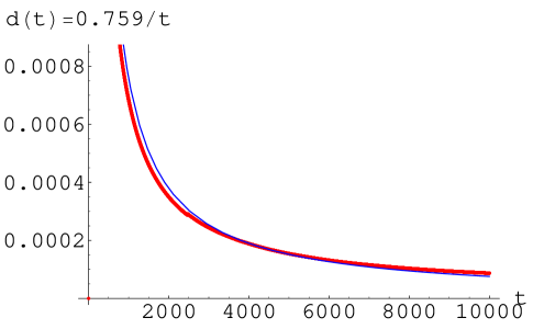
Figure 1: (Color online)The Dissipative Coupling Constant $\Delta(l_{t})$ : We show two graphs one is the R.G. result and the second is the fit to the analytic form $d(t)=0.7588/t\equiv d_{1}/t$

X COMPUTATION OF THE PARAMETRIC GREEN’S FUNCTION $D$ FOR TIMES $\tau\leq T$

Using the R.G. results from the previous section we will compute the hole type parametric Greens function for parallel spins $D^{(-)}[\omega,\epsilon;\widehat{g}=-i(u+i\Delta)]\equiv D^{(-)}[\omega,\epsilon;u,\Delta]$, where $\epsilon$ is the energy excitation perpendicular to the Fermi Surface $\epsilon=\vec{v_{F}}\cdot(\vec{K}-\vec{K_{F}}(s))$.

This Greens function $D^{(-)}[\omega,\epsilon;u,\Delta]$ is computed using the unperturbed Green’s function $D^{(-)}_{0}[\omega,\epsilon]$

$$(D^{(-)}[\omega,\epsilon;u,\Delta,E])^{-1}=(D^{(-)}_{0}[\omega,\epsilon])^{-1}+\Sigma[\omega,\epsilon;u,\Delta,E]$$

$$=\omega-\epsilon-\delta{\mu_{F}}+\Sigma[0,0;u,\Delta,E]+\omega\frac{d\Sigma[\omega,\epsilon;u,\Delta,E]}{d\omega}$$ (66)

where $\Sigma[\omega,\epsilon;u,\Delta,E]$ is the self energy. Using the fact that the R.G. equation has an infrared fixed point we can tune the shift in the chemical potential $\delta{\mu_{F}}(s)$ such that $\delta{\mu_{F}}(s)=\Sigma[0,0;u(l_{t})\approx u^{*}\approx\frac{u_{1}}{t},\Delta(l_{t})\approx\Delta^{*}\approx\frac{d_{1}}{t},E]$.

We obtain the wave function renormalization $Z_{\psi}(u(l_{t}))=e^{-\int_{0}^{{}_{t}}u(l^{\prime})\,dl^{\prime}}$. In the present case we stop scaling at $e^{l}\equiv v_{F}\Lambda T\equiv t$ and we find:

$$Z_{\psi}[u(l=log(t)=l_{t})]=e^{-\int_{0}^{l=log(t)=l_{t})}u(l^{\prime})\,dl^{\prime}}\approx e^{-\frac{u_{1}}{t}}$$ (67)

As a result we obtain the finite size Green’s function for $t>>1$ with the universal parameters $u_{1}$ and $d_{1}$: $D^{(-)}[\omega,\epsilon;u(l_{t}),\Delta(l_{t}),E]=\frac{e^{-u(l_{t})}}{\omega-\epsilon+i\omega\frac{\Delta(l_{t})}{2\pi}}\approx\frac{e^{-\frac{u_{1}}{t}}}{\omega-\epsilon+i\omega\frac{d_{1}}{2\pi t}}$. The action in eq.$(57)$ is restricted for large time intervals $T>\frac{2\pi}{v_{F}\Lambda}$ for which we can replace $e^{-\frac{u_{1}}{t}}\rightarrow 1$.

The parametric Green’s function which is restricted to the frequency interval $\frac{2\pi}{T}<\omega<v_{F}\Lambda$ is given by:

$$D[\omega,\epsilon;u(l_{t}),\Delta(l_{t}),E]=\frac{\vartheta[\epsilon]}{\omega-\epsilon+i\delta}+\frac{\vartheta[-\epsilon]}{\omega-\epsilon+i\omega\frac{d_{1}}{2\pi t}}$$ (68)

XI COMPUTATION OF THE PHYSICAL GREEN’S FUNCTION $G$

The Physical Green’s function $G$ will be computed from the Fourier representation of the parametric Green’s function $D$ given by equation $(68)$. We substitute in equation $(62)$ the explicit form of the parametric Green’s function $D[w,\epsilon]=D_{Re}[w,\epsilon]+iD_{Im}[w,\epsilon]$ as given in equation $(68)$ .

Using the Fourier transform of equation $62$ we find that the Green’s function $G$ is given in terms of two $new$ $functions$ $F_{R}(t;\omega,\epsilon)$ and $F_{Im}(t;\omega,\epsilon)$ which are a linear combination of the real and imaginary part of the parametric Green’s function $D^{(-)}[w,\epsilon]=D^{(-)}_{Re}[w,\epsilon]+iD^{(-)}_{Im}[w,\epsilon]$.

$G^{(-)}_{Re}[w,\epsilon]=\int_{\frac{2\pi}{v_{F}\Lambda}}^{T}F_{R}(t;\omega,\epsilon)\,dt$

$G^{(-)}_{Im}[w,\epsilon]=\int_{\frac{2\pi}{v_{F}\Lambda}}^{T}F_{Im}(t;\omega,\epsilon)\,dt$

where

$$F_{R}(t;\omega,\epsilon) = \int_{\frac{2\pi}{T}}^{v_{F}\Lambda}\frac{d\varpi}{2\pi}[D^{(-)}_{Re}[\varpi,\epsilon]Cos((\omega-\varpi)t)-D^{(-)}_{Re}[-\varpi,\epsilon]Cos((\omega+\varpi)t)]$$ (69)

$$-\int_{\frac{2\pi}{T}}^{v_{F}\Lambda}\frac{d\varpi}{2\pi}[D^{(-)}_{Im}[\varpi,\epsilon]Sin((\omega-\varpi)t)-D^{(-)}_{Im}[-\varpi,\epsilon]Sin((\omega+\varpi)t)]$$

$$F_{Im}(t;\omega,\epsilon) = \int_{\frac{2\pi}{T}}^{v_{F}\Lambda}\frac{d\varpi}{2\pi}[D^{(-)}_{Re}[\varpi,\epsilon]Sin((\omega-\varpi)t)-D^{(-)}_{Re}[-\varpi,\epsilon]Sin((\omega+\varpi)t)]$$ (70)

$$-\int_{\frac{2\pi}{T}}^{v_{F}\Lambda}\frac{d\varpi}{2\pi}[D^{(-)}_{Im}[\varpi,\epsilon]Cos((\omega-\varpi)t)-D^{(-)}_{Im}[-\varpi,\epsilon]Cos((\omega+\varpi)t)]$$

The Physical Green’s function $G[\omega,\epsilon=\vec{v_{F}}\cdot(\vec{K}-\vec{K_{F}}(s));E=v_{F}\Lambda]$ is given in terms of the self energy $\Sigma(\omega,\epsilon)=\Sigma_{Re}(\omega,\epsilon)+i\Sigma_{Im}(\omega,\epsilon)$.

$$G[\omega,\epsilon;E]=\frac{\vartheta[\epsilon]}{\omega-\epsilon+i\delta}+\frac{\vartheta[-\epsilon]}{\omega-\epsilon+\Sigma_{Re}(\omega)+i\Sigma_{Im}(\omega)}$$ (71)

In the present case equations $(69)$ and $(70)$ gives us the Physical Green’s in terms of the parametric Green’s function $D$. We represent the self energies of $G$ in terms of the parametric Green’s function. We find that:

$\Sigma_{Re}(\omega,\epsilon;z)=G_{Re}[w,\epsilon;z]/((G_{Re}[w,\epsilon;z])^{2}+(G_{Im}[w,\epsilon;z])^{2})-w$

and

$\Sigma_{Im}(\omega,\epsilon;z)=-G_{Im}[w,\epsilon;z]/((G_{Re}[w,\epsilon;z])^{2}+(G_{Im}[w,\epsilon;z])^{2})-z$ where $z\rightarrow 0$

where $G_{Re}[w,\epsilon]$ and $G_{Im}[w,\epsilon]$ are given by the equations $(69)-(70)$ .

The results for the self energy are given in figures 2 and 3 at a fixed energy $\epsilon=0$. (The Green’s function will be given as a function of dimensionless frequency and energy $\frac{\omega}{E=v_{F}\Lambda}\rightarrow\omega$ and $\frac{\epsilon}{E=v_{F}\Lambda}\rightarrow\epsilon$.) We observe that with increasing frequency the calculation of the self energy at energy $\epsilon=0$ becomes less accurate. For larger frequencies we have to compute $\Sigma_{Re}(\omega,\epsilon)$ and $\Sigma_{Im}(\omega,\epsilon)$ at finite energies $\epsilon$.

The self energy $\Sigma_{Im}(\omega)\propto\omega F(\frac{\omega}{v_{F}\Lambda})$ is linear in frequency for $\omega\rightarrow 0$. The function $F(\frac{\omega}{v_{F}\Lambda})$ represents the crossover from $1$ when $\omega\rightarrow 0$ to $\omega$ for increasing frequencies. When doping increases, the bandwidth $v_{F}\Lambda$ decreases and we observe that the linear region in frequency shrinks to $0$. As a result $\Sigma_{Im}(\omega)$ is modified to the Fermi liquid behavior $\Sigma_{Im}(\omega)\propto\omega^{2}$.

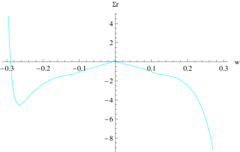
Figure 2: (Color online)The real part of the self energy self energy of the physical Green’s function $G(\omega,\epsilon)$ computed from the finite size Green’s function $D(\omega,\epsilon;u(l_{t}),\Delta(l_{t}),E)$

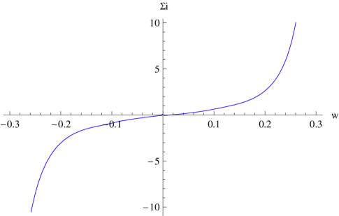
Figure 3: (Color online)The Imaginary part of the self energy of the physical Green’s function $G(\omega,\epsilon)$ computed from the finite size Green’s function $D(\omega,\epsilon;u(l_{t}),\Delta(l_{t}),E)$

Figure $3$ shows that the imaginary part of the self energy for low holes densities is linear in frequency. As a result, the single hole excitation (at low frequencies) has a width which is linear in frequency, and the scattering rate obeys $\frac{1}{\tau}\propto\omega F(\frac{\omega}{v_{F}\Lambda})$ in agreement with the infrared data Schlesinger .

XII APPLICATION OF THE THEORY TO SUPERCONDUCTIVITY

In this section we will attempt to connect the theory presented with the physics of the high $T_{c}$ material. In particular we have considered a model at $zero$ $temperature$ away from half fillings where the magnetic order has $vanished$. Under this condition we have shown that the marginal Fermi liquid with an imaginary self energy which is linear in frequency is obtained. This results are in agreement with the experiments which show that at T=0 a window exists between the magnetic ordered state and the appearance of superconductivity. Therefore, when the exchange interaction is included a d-wave superconducting hdavid phase within the exclusion of double occupancy will appear. The $d-wave$ order parameter $\sum_{\vec{a}}[\mathbf{\psi}_{\uparrow}(\vec{x})\mathbf{\psi}_{\downarrow}(\vec{x}+\vec{a})-\mathbf{\psi}_{\downarrow}(\vec{x})\mathbf{\psi}_{\uparrow}(\vec{x}+\vec{a})]|\Psi^{0}>\neq 0$ ($contrarily$ to the $s-wave$) is compatible with constraints $\mathbf{\psi}_{\uparrow}(\vec{x})\mathbf{\psi}_{\downarrow}(\vec{x})|\Psi^{0}>=0$. Further doping of the superconductor at T=0 will give rise to a transition from a free vortex monopole phase to a spin wave phase FSch .

For the remaining part of this section we will show that the effect of exclusion of double occupancy gives rise in the superconducting phase to an asymmetry in the tunneling density of states. In order to demonstrate the asymmetry effect of the projection of double occupancy we consider a qualitative calculation for superconductors . Strictly speaking an accurate comparison with the experiment must use the full $d$ wave structure. In order to demonstrate the effect of asymmetry induced by the projection, it is important to show that the asymmetry can be obtained also for an uniform state. We consider the standard $BCS$ hamiltonian and use the projection introduced in the previous sections. In the absence of the projection the effect of the $BCS$ gap $\Delta_{BCS}$ gives rise (after integration over the single particle energy) to the following $tunneling$ $density$ of $states$, $N_{T}^{(S-wave)}(\omega)=\frac{2}{\pi}\frac{K_{F}}{v_{F}}(\frac{-1}{2\pi})\int d\epsilon Im.G^{0-S}(\epsilon,\omega)$:

$$N_{T}^{(S-wave)}(\omega)=\frac{2}{\pi}\frac{K_{F}}{v_{F}}\frac{1}{\pi}\int_{0}^{1}\,d\epsilon[(1+\frac{\epsilon}{\sqrt{\epsilon^{2}+\Delta_{BCS}^{2}}})(\frac{z}{(\omega-\sqrt{\epsilon^{2}+\Delta_{BCS}^{2}})^{2}+z^{2}})$$

$$+(1+\frac{\epsilon}{\sqrt{\epsilon^{2}+\Delta_{BCS}^{2}}})(\frac{z}{(\omega+\sqrt{\epsilon^{2}+\Delta_{BCS}^{2}})^{2}+z^{2}})]$$ (72)

where $z\rightarrow 0$.

Next we repeat the calculation when we project out double occupancy! For this purpose we use the $self$ $energy$ given in figure $3$, $\Sigma_{Im}(\omega)$.

The tunneling density of states for the $projected$ case of double occupancy is given by $N_{T}^{(S-w.ex.)}(\omega)$:

$$N_{T}^{(S-w.ex.)}(\omega)=\frac{2}{\pi}\frac{K_{F}}{v_{F}}\frac{1}{\pi}\int_{0}^{1}\,d\epsilon[(1+\frac{\epsilon}{\sqrt{\epsilon^{2}+\Delta_{BCS}^{2}}})(\frac{z}{(\omega-\sqrt{\epsilon^{2}+\Delta_{BCS}^{2}})^{2}+z^{2}})$$

$$+(1+\frac{\epsilon}{\sqrt{\epsilon^{2}+\Delta_{BCS}^{2}}})(\frac{\Sigma_{Im}(\omega)}{(\omega+\sqrt{\epsilon^{2}+\Delta_{BCS}^{2}})^{2}+(\Sigma_{Im}(\omega))^{2}})]$$ (73)

where $z\rightarrow 0$.

In order to emphasize the asymmetric effect of the self energy we consider typical values of temperatures and gap. For the gap we take the value $\Delta_{BCS}=0.38\times 10^{-3}$ eV and restrict the temperature to, $T_{B}<\Delta_{BCS}$.

In figure $4$ we show the two graphs of the tunneling density of states, $N_{T}^{(S-wave)}(\omega=\frac{eV}{\hbar})$ is the tunneling density of states in the absence of projection and $N_{T}^{(S-w.ex.)}(\omega=\frac{eV}{\hbar})$ is the tunneling density of states for the projected case. The tunneling density of states as a function of the tunneling voltage $V$ shows a clear asymmetry between the projected $N_{T}^{(S-w.ex.)}$ and the non - projected function $N_{T}^{(S-wave)}$.

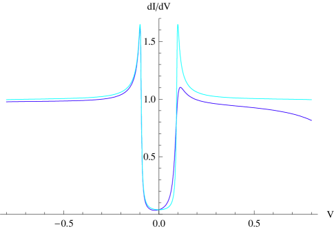
Figure 4: (Color online)a)-The tunneling density of states for S-wave superconductivity as a function of the voltage $V$ without projection $N_{T}^{(S-wave)}(\frac{eV}{\hbar})$ b)-The tunneling density of states for S-wave superconductivity as a function of the voltage $V$ with projection (the $asymmetric$ graph) $N_{T}^{(S-w.ex.)}(\frac{eV}{\hbar})$

In figure $5$ we show on the same graph: the experimental data for the tunneling of the density states observed in Pan and our projected tunneling density of states. Figure $5$ demonstrates that the asymmetry in the tunneling density of states can be explained by the projected Green’s function.

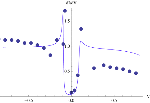
Figure 5: (Color online)The tunneling density of states given by the dots extracted from the experiment in ref. Pan compared to the analytic formula for the projected tunneling density of states $N_{T}^{(S-w.ex.)}(\frac{eV}{\hbar})$

XIII CONCLUSION

We have proposed a new method to study correlated electrons where the traditional method of slave particles is avoided. We have demonstrated that by choosing proper variables additional constraints can be included. We obtain a system of first class constraints which generate gauge transformations.

The authors Muthu ; Gutz have computed the wave function using only one constraint. We identify two additional constraints which form an non-Abelian group and neglect according to the R.G. analysis the secondary constraints. As a result the simple delta function constraint is replaced by a non-linear integration measure which gives rise to time dependent action.

The effective action is analyzed with the help of the R.G.method for finite size systems (in the time domain).

The R.G. analysis allows to compute the single particle self energy which is used for $qualitative$ comparison with the experiments.

APPENDIX:THE SECONDARY FIRST CLASS CONSTRAINTS

In this Appendix we will show that the effective interactions induced by the secondary first class constraints are irrelevant operators for describing the long low energy Physics and therefore can be neglected.

In order to show this we perform the followings steps:

A1) Compute the commutator of the kinetic energy with the primary first class constraints. (In the absence of the exchange interaction, the hamiltonian is given by $H_{0}$.)

$[\mathbf{\psi}_{\sigma=\downarrow}(\vec{x})\mathbf{\psi}_{\sigma=\uparrow}(\vec{x}),H_{0}]=t\sum_{\vec{a}}[\mathbf{\psi}_{\sigma=\downarrow}(\vec{x})\mathbf{\psi}_{\sigma=\uparrow}(\vec{x}+\vec{a})+\mathbf{\psi}_{\sigma=\downarrow}((\vec{x}+\vec{a}))\mathbf{\psi}_{\sigma=\uparrow}(\vec{x})]$

The secondary constraints $q(\vec{x})$, $q^{+}(\vec{x})$ and $q_{3}(\vec{x})$ are obtained by commuting the primary constraints with the hamiltonian $H_{0}$ and subtracting the primary constraints:

$q(\vec{x})\equiv\frac{1}{t}[Q(\vec{x}),H_{0}]-Q(\vec{x})=\sum_{\vec{a}}[\mathbf{\psi}_{\sigma=\downarrow}(\vec{x})\mathbf{\psi}_{\sigma=\uparrow}(\vec{x}+\vec{a})+\mathbf{\psi}_{\sigma=\downarrow}((\vec{x}+\vec{a}))\mathbf{\psi}_{\sigma=\uparrow}(\vec{x})]-Q(\vec{x})$

$q^{+}(\vec{x})\equiv\frac{1}{t}[Q^{+}(\vec{x}),H_{0}]-Q^{+}(\vec{x})=\sum_{\vec{a}}[\mathbf{\psi}_{\sigma=\downarrow}(\vec{x})\mathbf{\psi}_{\sigma=\uparrow}(\vec{x}+\vec{a})+\mathbf{\psi}_{\sigma=\downarrow}((\vec{x}+\vec{a}))\mathbf{\psi}_{\sigma=\uparrow}(\vec{x})]^{+}-Q^{+}(\vec{x})$

and

$q_{3}(\vec{x})\equiv\frac{1}{t}[Q_{3}(\vec{x}),H_{0}]-[Q_{3}(\vec{x})-1)]=\sum_{\vec{a}}[\mathbf{\psi}_{\sigma=\downarrow}(\vec{x})\mathbf{\psi}_{\sigma=\downarrow}(\vec{x}+\vec{a})+\mathbf{\psi}_{\sigma=\uparrow}((\vec{x}+\vec{a}))\mathbf{\psi}_{\sigma=\uparrow}(\vec{x})]-[Q_{3}(\vec{x})-1]$

A2) In section VII we have parametrized Fermi-Surface in terms of the polar angle $s$, normal $\hat{N}(s)$ to the Fermi Surface and chiral fermions $R_{\sigma}(\vec{x},s)$, ,$L_{\sigma}(\vec{x},s)$ .The hamiltonian $H_{0}$ is given by:

$H_{0}=\int d^{2}x\int_{0}^{\pi}\frac{ds}{\pi}\sum_{\sigma=\uparrow,\downarrow}[R^{\dagger}_{\sigma}(\vec{x};s)(-iv_{F}\hbar)\hat{N}(s)\cdot\vec{\partial}_{\vec{x}}R_{\sigma}(\vec{x};s)+L^{\dagger}_{\sigma}(\vec{x};s)(iv_{F}\hbar)\hat{N}(s)\cdot\vec{\partial}_{\vec{x}}L_{\sigma}(\vec{x};s)]$

A3) Approximating the difference between the commutators and the primary constraints by a first order spatial derivative around the Fermi-Surface we obtain:

$q(\vec{x})\approx\int_{0}^{\pi}\frac{ds}{\pi}[R_{\uparrow}(\vec{x},s)\hat{N}(s)\cdot\vec{\partial}_{\vec{x}}L_{\downarrow}(\vec{x},s)-L{\downarrow}(\vec{x},s)\hat{N}(s)\cdot\vec{\partial}_{\vec{x}}R_{\downarrow}(\vec{x},s)]$

$q^{+}(\vec{x})\approx[\int_{0}^{\pi}\frac{ds}{\pi}[R_{\uparrow}(\vec{x},s)\hat{N}(s)\cdot\vec{\partial}_{\vec{x}}L_{\downarrow}(\vec{x},s)-L{\downarrow}(\vec{x},s)\hat{N}(s)\cdot\vec{\partial}_{\vec{x}}R_{\downarrow}(\vec{x},s)]]^{+}$

and

$q_{3}(\vec{x})\approx\int_{0}^{\pi}\frac{ds}{\pi}[R^{+}_{\uparrow}(\vec{x},s)\hat{N}(s)\cdot\vec{\partial}_{\vec{x}}R_{\uparrow}(\vec{x},s)+L^{+}{\downarrow}(\vec{x},s)\hat{N}(s)\cdot\vec{\partial}_{\vec{x}}L_{\downarrow}(\vec{x},s)]$.

A4) The presence of the secondary constraints the modifies the Lagrangian $L\Rightarrow L+\delta L$ where $\delta L$ is given by:

$\delta L=\sum_{r=1}^{3}\hat{\pi}_{r}(\vec{x},t)\partial_{t}\hat{\lambda}^{r}(\vec{x},t)-\sum_{r=1}^{3}(\hat{\pi}_{r}(\vec{x},t)\hat{\chi}^{r}(\vec{x},t)+\hat{\lambda}^{r}(\vec{x},t)q^{(-)}_{r}(\vec{x},t))$

where $\hat{\lambda}^{r}(\vec{x},t)$ are the Lagrange multipliers which enforces the secondary constraints, $\hat{\pi}_{r}(\vec{x},t)$ are the canonical momentum conjugate to the new Lagrange $\hat{\lambda}^{r}(\vec{x},t)$ multipliers and $q^{(-)}_{r}(\vec{x},t))$ are obtained using the linear transformation given in equations $(35)$ and $(36)$. This gives rise to the evolution operator:

$\hat{U}_{phys}[t_{f},t_{i}]=e^{\frac{-i}{\hbar}(t_{f}-t_{i})H}\int\prod_{\alpha=1}^{3}\mathcal{D}\lambda_{\alpha}(T)\prod_{r=1}^{3}\mathcal{D}\hat{\lambda}_{r}(T)e^{\frac{-i}{{\hbar}}\left[\sum_{\alpha=1}^{3)}\int\lambda_{\alpha}(\vec{x})Q^{-}_{\alpha}(\vec{x})\,d^{d}x+\sum_{r=1}^{3)}\int\hat{\lambda}_{r}(\vec{x})q^{(-)}_{r}(\vec{x}))\,d^{d}x\right]}$

In order to compute the effective interaction induced by the secondary constraints we need the integration measure for the secondary Lagrange multipliers $\hat{\lambda}^{r}(\vec{x},t)$. We approximate the measure by a regular integration and obtain a set of delta functions which enforces the constraints $q^{(-)}_{r}(\vec{x},t))$. The delta functions constraints effectively replaced by exponentials of Gaussian terms with the coupling constant $\delta g_{I}$ ( which at short distances goes to infinity and therefore is equivalent to a delta function). The Gaussian action is given by; $\delta g_{I}\sum_{r=1}^{3}\int d^{d}x\int dt_{1}\int dt_{2}[q^{(-)}_{r}(\vec{x},t_{1}))q^{(-)}_{r}(\vec{x},t_{2}))]$. As a result, we obtain the correction $\delta S^{eff-hole}_{int.}[\widehat{t_{i}},\widehat{t_{f}}]$ to the original action given in eq.$(57)$:

$$\delta S^{eff-hole}_{int.}[\widehat{t_{i}},\widehat{t_{f}}] = \int_{0}^{\pi}\frac{ds_{1}}{\pi}\int_{0}^{\pi}\frac{ds_{2}}{\pi}\int_{\widehat{t_{i}}}^{\widehat{t_{f}}}\,dt_{1}\int_{\widehat{t_{i}}}^{\widehat{t_{f}}}\,dt_{2}\prod_{n=1}^{4}\frac{d\epsilon_{n}}{(2\pi)^{3}}\widehat{J}[\epsilon_{1},s_{1}]\widehat{J}[\epsilon_{2},s_{2}]$$

$$\delta g_{I}\delta(-\epsilon_{1}+\epsilon_{2}+\epsilon_{3}-\epsilon_{4})$$

$$[[R^{\dagger(-)}_{\downarrow}(t_{1},-\epsilon_{1};s_{1})(\epsilon_{2})L^{\dagger(-)}_{\uparrow}(t_{1},\epsilon_{2};s_{1})L^{(-)}_{\uparrow}(t_{2},\epsilon_{3};s_{2})(-\epsilon_{4})R^{(-)}_{\downarrow}(t_{2},-\epsilon_{4};s_{2})$$

$$+L^{\dagger(-)}_{\downarrow}(t_{1},\epsilon_{1};s_{1})(-\epsilon_{2})R^{\dagger(-)}_{\uparrow}(t_{1},-\epsilon_{2};s_{1})L^{(-)}_{\uparrow}(t_{2},\epsilon_{3};s_{2})(-\epsilon_{4})R{(-)}_{\downarrow}(t_{2},-\epsilon_{4};s_{2})]$$

$$+[R^{\dagger(-)}_{\downarrow}(t_{1},-\epsilon_{1};s_{1})(-\epsilon_{1})L^{\dagger(-)}_{\uparrow}(t_{1},\epsilon_{2};s_{1})R^{(-)}_{\uparrow}(t_{2},-\epsilon_{3};s_{2})(\epsilon_{4})L^{(-)}_{\downarrow}(t_{2},\epsilon_{4};s_{2})+$$

$$L^{\dagger(-)}_{\downarrow}(t_{1},\epsilon_{1};s_{1})(\epsilon_{1})R^{\dagger(-)}_{\uparrow}(t_{1},-\epsilon_{2};s_{1})L^{(-)}_{\uparrow}(t_{2},\epsilon_{3};s_{2})(-\epsilon_{4})R^{(-)}_{\downarrow}(t_{2},-\epsilon_{4};s_{2})]]....$$

The spatial derivatives in the last equation are replaced by the energy excitations normal to the Fermi Surface $\epsilon$. As a result, the engineering dimensions of the coupling constants $\delta g$ is given by:         $\delta g_{I}=\delta\widehat{g}_{I}v_{F}E^{-1}$.

The presence of two spatial derivatives and the two time integrations generate the engineering dimensions $E^{-1}$. Therefore we will ignore $\delta S^{eff-hole}_{int.}$ for describing the Physics at $low$ $energies$. (The Physics at $short$ $distances$ is sensitive to operators which have negative scaling dimensions and therefore can not be ignored.)

References

- (1) M. Ogata and H. Shiba, Phys. Rev. B 41 2326(1990)
- (2) R.O.Zaitsev,Sov.Phys.JETP 48,1183(1988).
- (3) S.E.Barnes,J.Phys.F 6,1375(1976)
- (4) D.Schmeltzer ,Phys.Rev.B 38,8923(1988);
- (5) P.B.Wiegmann,Phys.Rev.Lett.60,821(1988).
- (6) P. A. Lee, N. Nagaosa, X. G. Wen, Cond-Matt/0410445 .
- (7) P. W. Anderson, Science, 235 1196(1987)
- (8) D. Schmeltzer and A. Bishop, J. Phys:Condens Matter 16 7753(2004).
- (9) T. Senthil and M. Fisher, Phys. Rev. B 62 7850(2000)
- (10) Chetan Nayak ,Phys.Rev.Lett. 95,178,(2000)
- (11) D.Schmeltzer ,Phys.Rev.B 43,8650(1990)
- (12) Eberhard O.Tungler and Thilo Kopp Cond-mat/9412092.
- (13) M.C. Gutzwiller ,Physical Review Letters 10,159 (1963).
- (14) Bernhard Edeggeer, V.N.Muthukumar,Claudio Gross Cond-mat/2007.1020v1
- (15) P.W.Anderson Cond-mat/ 0510053
- (16) Lijun Zhu , Vivek Aji, Arkadi Shechter and C.M. Varma Cond-Matt/0702187 v2
- (17) Vivek Aji and C.M. Varma Cond-Matt/0610646
- (18) N. Doiron-Leyraud et al, 447, 565(2007).
- (19) S. R. Julian, M. R. Norman, Nature, 447 537(2007).
- (20) Paul A.M.Dirac ,”’Lectures On Quantum Mechanics”’,Dover Publications ,Inc.Mineola New York (2001).
- (21) Marc Henneaux and Claudio Teitelboim, ”‘Quantization of Gauge System”’ ,Princeton University Press ,Princeton,New Jersey (1992).
- (22) J.W.Holten ,hep-th/0201124.
- (23) D.Schmeltzer,J.Phys-Condens Matter 20,335205(2008).
- (24) D.Schmeltzer and H.Yeh Chang ,PMC Physics B 201:14,October 21.
- (25) Z.Schlesinger, R.T.Collins, F.Holtzberg, C.Feidl, S.H.Blanton, U.Welp, G.W.Crabtree, Y,fang,and J.Z. Liu Phys.Rev.Lett. 65,801 (1990)
- (26) D.Schmeltzer, Physics Letters A 293(2002) 74-82.
- (27) S.H.Pan et al., Nature , 746,(2000)
- (28) M.Kugler ,O.Fisher ,Ch.Renner ,S.Ono and Yoichi Ando Phys.Rev.Lett.86,4911,(2001).
- (29) E.S. Fradkin and G.A. Vilkovisky Physics Letters 55B,224(1975).
- (30) I.A. Batalin and E.S.Fradkin Physics Letter 128B,303 (1983).
- (31) R.Fulp math/060427.
- (32) D.Schmeltzer ,Phys.Rev.B 52,7939(1995)
- (33) P.Kopietz and T.Busche ,Phys.Rev.B 64,155101(2001)
- (34) E.Brezin Journal de Physique (Paris) 43,15,(1982).
- (35) S.L.Sondhi,S.M.Girvin, J.P.Carin and D.Shahar, Rev.of Modern Physics 69,315,(1997).
- (36) John R.Klauder, ”‘Quantization of Constrained Systems”’ Lect. Notes Phys. 572,143 (2001)
- (37) Claude Itzykson and Jean-Bernard Zuber ,”’Quantum Field Theory ”‘ section 9.3 and 12-2-2Dover Publications,Inc.Mineola, NY .
- (38) Claude Itzykson and Jean-Bernard Zuber , ”’Quantum Field Theory ”‘ section 9-1-3 Dover Publications,Inc.Mineola, NY.
- (39) L.D. Faddev and A.A. Slavnov ,”’Gauge fields An introduction To quantum Theory”’ chapter 3, Addison -Wesley Publishing Company .
- (40) A. Foussats , A. Greco, C. Repettto, O.P. Zandron and O.S. Zandron J.Phys.A:Math.Gen. 33,5849(2000)
- (41) A.Fetter and J.D.Walecka , ”‘Quantum Theory of Many-Particle Systems”’, Dover Publications (1971).
- (42) G.Reinhardt,”’Field Quantization”’ pages 356-363, Springer-Verlag 1993.
- (43) R.Shankar ,Review of Modern Physics 66,129(1994)
- (44) J.Polchinsky ,NSF-ITP-92-132 ,UTTG-20-92 .
- (45) M.Nakhara ,Geometry,Topology and Physics ,Taylor Francis 2003, pages 36-38
- (46) B. Hartfield ,Quantum Field Theory of Point Particles and Strings,Addison Wesley 1992, pages 611-616.