Homogenization with large spatial random potential

Abstract

We consider the homogenization of parabolic equations with large spatially-dependent potentials modeled as Gaussian random fields. We derive the homogenized equations in the limit of vanishing correlation length of the random potential. We characterize the leading effect in the random fluctuations and show that their spatial moments converge in law to Gaussian random variables. Both results hold for sufficiently small times and in sufficiently large spatial dimensions $d\geq{\mathfrak{m}}$, where ${\mathfrak{m}}$ is the order of the spatial pseudo-differential operator in the parabolic equation. In dimension $d<{\mathfrak{m}}$, the solution to the parabolic equation is shown to converge to the (non-deterministic) solution of a stochastic equation in the companion paper [2]. The results are then extended to cover the case of long range random potentials, which generate larger, but still asymptotically Gaussian, random fluctuations.

keywords:

Homogenization theory, partial differential equations with random coefficients, Gaussian fluctuations, large potential, long range correlations

AMS:

35R60, 60H05, 35K15.

1 Introduction

Let ${\mathfrak{m}}>0$ and $P(D)$ the pseudo-differential operator with symbol $\hat{p}(\xi)=|\xi|^{\mathfrak{m}}$. We consider the following evolution equation in dimension $d\geq{\mathfrak{m}}$:

$$\begin{array}[]{rcll}\Big{(}\dfrac{\partial{}}{\partial{t}}+P(D)-\dfrac{1}{\varepsilon^{\alpha}}q\big{(}\dfrac{x}{\varepsilon}\big{)}\Big{)}u_{\varepsilon}(t,x)&=&0,&x\in\mathbb{R}^{d},\quad t>0,\\ u_{\varepsilon}(0,x)&=&u_{0}(x),&x\in\mathbb{R}^{d}.\end{array}$$ (1)

Here, $u_{0}\in L^{2}(\mathbb{R}^{d})$ and $q(x)$ is a mean zero stationary Gaussian process defined on a probability space $(\Omega,\mathcal{F},\mathbb{P})$. We assume that $q(x)$ has bounded and integrable correlation function $R(x)=\mathbb{E}\{q(y)q(x+y)\}$, where $\mathbb{E}$ is the mathematical expectation associated with $\mathbb{P}$, and bounded, continuous in the vicinity of $0$, and integrable power spectrum $(2\pi)^{d}\hat{R}(\xi)=\int_{\mathbb{R}^{d}}e^{-i\xi\cdot x}R(x)dx$ in the sense that $\int_{\mathbb{R}^{d}\backslash B(0,1)}\hat{R}(\xi)|\xi|^{-{\mathfrak{m}}}d\xi<\infty$. The size of the potential is constructed so that the limiting solution as $\varepsilon\to 0$ is different from the unperturbed solution obtained by setting $q=0$. The appropriate size of the potential is given by

$$\varepsilon^{\alpha}=\left\{\begin{matrix}\varepsilon^{\frac{{\mathfrak{m}}}{2}}|\ln\varepsilon|^{\frac{1}{2}}&d={\mathfrak{m}},\\ \varepsilon^{\frac{{\mathfrak{m}}}{2}}&d>{\mathfrak{m}}.\end{matrix}\right.$$ (2)

The potential is bounded $\mathbb{P}$-a.s. on bounded domains but is unbounded $\mathbb{P}$-a.s. on $\mathbb{R}^{d}$. By using a method based on the Duhamel expansion, we nonetheless obtain that for a sufficiently small time $T>0$, the above equation admits a weak solution $u_{\varepsilon}(t,\cdot)\in L^{2}(\Omega\times\mathbb{R}^{d})$ uniformly in time $t\in(0,T)$ and $0<\varepsilon<\varepsilon_{0}$.

Moreover, as $\varepsilon\to 0$, the solution $u_{\varepsilon}(t)$ converges strongly in $L^{2}(\Omega\times\mathbb{R}^{d})$ uniformly in $t\in(0,T)$ to its limit $u(t)$ solution of the following homogenized evolution equation

$$\begin{array}[]{rcll}\Big{(}\dfrac{\partial{}}{\partial{t}}+P(D)-\rho\Big{)}u(t,x)&=&0,&x\in\mathbb{R}^{d},\quad t>0,\\ u(0,x)&=&u_{0}(x),&x\in\mathbb{R}^{d},\end{array}$$ (3)

where the effective (non-negative) potential is given by

$$\rho=\left\{\begin{array}[]{ll}\,\,c_{d}\hat{R}(0)&d={\mathfrak{m}},\\[0.0pt] \displaystyle\int_{\mathbb{R}^{d}}\dfrac{\hat{R}(\xi)}{|\xi|^{\mathfrak{m}}}d\xi&d>{\mathfrak{m}}.\end{array}\right.$$ (4)

Here, $c_{d}$ is the volume of the unit sphere $S^{d-1}$. We denote by $\mathcal{G}^{\rho}_{t}$ the propagator for the above equation, which to $u_{0}(x)$ associates $\mathcal{G}^{\rho}_{t}u_{0}(x)=u(t,x)$ solution of (3).

We assume that the non-negative (by Bochner’s theorem) power spectrum $\hat{R}(\xi)$ is bounded by $f(|\xi|)$, where $f(r)$ is a positive, bounded, radially symmetric, and integrable function in the sense that $\int_{1}^{\infty}r^{d-1-{\mathfrak{m}}}f(r)dr<\infty$. Then we have the following result.

Theorem 1

There exists a time $T=T(f)>0$ such that for all $t\in(0,T)$, there exists a solution $u_{\varepsilon}(t)\in L^{2}(\Omega\times\mathbb{R}^{d})$ uniformly in $0<\varepsilon<\varepsilon_{0}$. Moreover, let us assume that $\hat{R}(\xi)$ is of class $\mathcal{C}^{\gamma}(\mathbb{R}^{d})$ for some $0\leq\gamma\leq 2$ and let $u(t,x)$ be the unique solution in $L^{2}(\mathbb{R}^{d})$ to (3). Then, we have the convergence results

$$\begin{array}[]{rcl}\|(u_{\varepsilon}-{\mathfrak{u}}_{\varepsilon})(t)\|_{L^{2}(\Omega\times\mathbb{R}^{d})}&\lesssim&\varepsilon^{\frac{\beta}{2}}\|u_{0}\|_{L^{2}(\mathbb{R}^{d})},\\[5.69054pt] \|({\mathfrak{u}}_{\varepsilon}-u)(t)\|_{L^{2}(\mathbb{R}^{d})}&\lesssim&\varepsilon^{\gamma\wedge\beta}\|u_{0}\|_{L^{2}(\mathbb{R}^{d})},\end{array}$$ (5)

where $a\lesssim b$ means $a\leq Cb$ for some $C>0$, $a\wedge b=\min(a,b)$, where ${\mathfrak{u}}_{\varepsilon}(t,\cdot)$ is a deterministic function in $L^{2}(\mathbb{R}^{d})$ uniformly in time, and where we have defined

$$\varepsilon^{\beta}=\left\{\begin{array}[]{lc}|\ln\varepsilon|^{-1}&d={\mathfrak{m}},\\ \varepsilon^{d-{\mathfrak{m}}}&{\mathfrak{m}}<d<2{\mathfrak{m}},\\ \varepsilon^{{\mathfrak{m}}}|\ln\varepsilon|&d=2{\mathfrak{m}},\\ \varepsilon^{{\mathfrak{m}}}&d>2{\mathfrak{m}}.\end{array}\right.$$ (6)

The Fourier transform ${\mathfrak{U}}_{\varepsilon}(t,\xi)$ of the deterministic function ${\mathfrak{u}}_{\varepsilon}(t,x)$ is determined explicitly in (58) below.

Note that the effective potential $-\rho$ is non-positive. The theorem is valid for times $T$ such that $4T\rho_{f}<1$, where $\rho_{f}$ is defined in lemma 2.2 below by replacing $\hat{R}(\xi)$ by $f(|\xi|)$ in the definition of $\rho$ in (4).

The error term $u_{\varepsilon}-u$ is dominated by deterministic components when $\varepsilon^{\gamma\wedge\beta}\gg\varepsilon^{\frac{d-2\alpha}{2}}$ and by random fluctuations when $\varepsilon^{\gamma\wedge\beta}\ll\varepsilon^{\frac{d-2\alpha}{2}}$. In both situations, the random fluctuations may be estimated as follows. We show that

$$u_{1,\varepsilon}(t,x)=\dfrac{1}{\varepsilon^{\frac{d-2\alpha}{2}}}\big{(}u_{\varepsilon}-\mathbb{E}\{u_{\varepsilon}\}\big{)}(t,x),$$ (7)

converges weakly in space and in distribution to a Gaussian random variable. More precisely, we have

Theorem 2

Let $M$ be a test function such that its Fourier transform $\hat{M}\in L^{1}(\mathbb{R}^{d})\cap L^{2}(\mathbb{R}^{d})$. Then we find that for all $t\in(0,T)$

$$(u_{1,\varepsilon}(t,\cdot),M)\xrightarrow{\,\varepsilon\to 0\,}\displaystyle\int_{\mathbb{R}^{d}}{\mathcal{M}}_{t}(x)\sigma dW_{x},\qquad\mathcal{M}_{t}(x)=\displaystyle\int_{0}^{t}\mathcal{G}^{\rho}_{s}M(x)\mathcal{G}^{\rho}_{t-s}u_{0}(x)ds,$$ (8)

where convergence holds in the sense of distributions, $dW_{x}$ is the standard multiparameter Wiener measure on $\mathbb{R}^{d}$ and $\sigma$ is the standard deviation defined by

$$\sigma^{2}:=(2\pi)^{d}\hat{R}(0)=\displaystyle\int_{\mathbb{R}^{d}}\mathbb{E}\{q(0)q(x)\}dx.$$ (9)

This shows that the fluctuations of the solution are asymptotically given by a Gaussian random variable, which is consistent with the central limit theorem.

We observe a sharp transition in the behavior of $u_{\varepsilon}$ at $d={\mathfrak{m}}$. For $d<{\mathfrak{m}}$, the following holds. The size of the potential that generates an order $O(1)$ perturbation is now given by (see the last inequality in lemma 2.2)

$$\varepsilon^{\alpha}=\varepsilon^{\frac{d}{2}}.$$

Using the same methods as for the case $d\geq{\mathfrak{m}}$, we may obtain that $u_{\varepsilon}(t)$ is uniformly bounded and thus converges weakly in $L^{2}(\Omega\times\mathbb{R}^{d})$ for sufficiently small times to a function $u(t)$. The problem is addressed in [2], where it is shown that $u(t)$ is the solution to the stochastic partial differential equation in Stratonovich form

$$\dfrac{\partial{u}}{\partial{t}}+P(D)u+u\circ\sigma\dfrac{d{W}}{d{x}}=0,$$ (10)

with $u(0,x)=u_{0}(x)$ and $\frac{dW}{dx}$ d-parameter spatial white noise “density”. The above equation admits a unique solution that belongs to $L^{2}(\Omega\times\mathbb{R}^{d})$ locally uniformly in time. Stochastic equations have also been analyzed in the case where $d\geq{\mathfrak{m}}$ (i.e., $d\geq 2$ when $P(D)=-\Delta$), see [9, 12]. However, our results show that such solutions cannot be obtained as a limit in $L^{2}(\Omega\times\mathbb{R}^{d})$ of solutions corresponding to vanishing correlation length so that their physical justification is more delicate. In the case $d=1$ and ${\mathfrak{m}}=2$ with $q(x)$ a bounded potential, we refer the reader to [13] for more details on the above stochastic equation.

The above theorems 1 and 2 assume short range correlations for the random potential. Mathematically, this is modeled by an integrable correlation function, or equivalently a bounded value for $\hat{R}(0)$. Longer range correlations may be modeled by unbounded power spectra in the vicinity of the origin, for instance by assuming that $\hat{R}(\xi)=h(\xi)\hat{S}(\xi)$, where $\hat{S}(\xi)$ is bounded in the vicinity of the origin and $h(\xi)$ is a homogeneous function of degree $-{\mathfrak{n}}$ for some ${\mathfrak{n}}>0$. Provided that $d>{\mathfrak{m}}+{\mathfrak{n}}$ so that $\rho$ defined in (4) is still bounded, the results of theorems 1 and 2 may be extended to the case of long range fluctuations. We refer the reader to theorem 3 in section 3.3 below for the details. The salient features of the latter result is that the convergence properties stated in theorem 1 still hold with $\beta$ replaced by $\beta-{\mathfrak{n}}$ and that the random fluctuations are now asymptotically Gaussian processes of amplitude of order $\varepsilon^{\frac{d-{\mathfrak{m}}-{\mathfrak{n}}}{2}}$. Moreover, they may conveniently be written as stochastic integrals with respect to some multiparameter fractional Brownian motion in place of the Wiener measure appearing in (8).

Let us also mention that all the result stated here extend to the Schrödinger equation, where $\frac{\partial}{\partial t}$ is replaced by $i\frac{\partial}{\partial t}$ in (1). We then verify that $-\rho$ in (3) is replaced by $\rho$ so that the homogenized equation is given by

$$\Big{(}i\dfrac{\partial{}}{\partial{t}}+P(D)+\rho\Big{)}u(t,x)\,=\,0.$$

The main effect of the randomness is therefore a phase shift of the quantum waves as they propagate through the random medium. Because the semigroup associated to the free evolution of quantum waves does not damp high frequencies as efficiently as for the parabolic equation (1), some additional regularity assumptions on the initial condition are necessary to obtain the limiting behaviors described in theorems 1 and 2. We do not consider the case of the Schrödinger equation further here.

The rest of the paper is structured as follows. Section 2 recasts (1) as an infinite Duhamel series of integrals in the Fourier domain. The cross-correlations of the terms appearing in the series are analyzed by calculating moments of Gaussian variables and estimating the contributions of graphs similar to those introduced in [5, 11]. These estimates allow us to construct a solution to (1) in $L^{2}(\Omega\times\mathbb{R}^{d})$ uniformly in time for sufficiently small times $t\in(0,T)$. The maximal time $T$ of validity of the theory depends on the power spectrum $\hat{R}(\xi)$. The estimates on the graphs are then used in section 3 to characterize the limit and the leading random fluctuations of the solution $u_{\varepsilon}(t,x)$. The extension of the results to long range correlations is presented in section 3.3.

The analysis of (1) and of similar operators has been performed for smaller potentials than those given in (2) in e.g. [1, 6] when $u_{\varepsilon}$ converges strongly to the solution of the unperturbed equation (with $q\equiv 0$). The results presented in this paper may thus be seen as generalizations to the case of sufficiently strong potentials so that the unperturbed solution is no longer a good approximation of $u_{\varepsilon}$. The analysis presented below is based on simple estimates for the Feynman diagrams corresponding to Gaussian random potentials and does not extend to other potentials such as Poisson point potentials, let alone potentials satisfying some mild mixing conditions. Extension to other potentials would require more sophisticated estimates of the graphs than those presented here or a different functional setting than the $L^{2}(\Omega\times\mathbb{R}^{d})$ setting considered here. For related estimates on the graphs appearing in Duhamel expansion, we refer the reader to e.g. [4, 5, 11].

2 Duhamel expansion and existence theory

Since $q(x)$ is a stationary mean zero Gaussian random field, it admits the following spectral representation

$$q(x)=\dfrac{1}{(2\pi)^{d}}\displaystyle\int_{\mathbb{R}^{d}}e^{i\xi\cdot x}\hat{Q}(d\xi),$$ (11)

where $\hat{Q}(d\xi)$ is the complex spectral process such that

$$\mathbb{E}\Big{\{}\displaystyle\int_{\mathbb{R}^{d}}f(\xi)\hat{Q}(d\xi)\overline{\displaystyle\int_{\mathbb{R}^{d}}g(\xi)\hat{Q}(d\xi)}\Big{\}}=\displaystyle\int_{\mathbb{R}^{d}}f(\xi)\bar{g}(\xi)(2\pi)^{d}\hat{R}(\xi)d\xi,$$

for all $f$ and $g$ in $L^{2}(\mathbb{R}^{d};\hat{R}(\xi)d\xi)$ with the power spectrum and correlation function of $q$ respectively defined by

$$0\leq(2\pi)^{d}\hat{R}(\xi)=\displaystyle\int_{\mathbb{R}^{d}}e^{-i\xi\cdot x}R(x)dx,\qquad R(x)=\mathbb{E}\{q(y)q(x+y)\}.$$ (12)

In the sequel, we write $\hat{Q}(d\xi)\equiv\hat{q}(\xi)d\xi$ so that $\mathbb{E}\{\hat{q}(\xi)\hat{q}(\zeta)\}=\hat{R}(\xi)\delta(\xi+\zeta)$ and $\mathbb{E}\{\hat{q}(\xi)\overline{\hat{q}(\zeta)}\}=\hat{R}(\xi)\delta(\xi-\zeta)$.

2.1 Duhamel expansion

Let us introduce $\hat{q}_{\varepsilon}(\xi)=\varepsilon^{d-\alpha}\hat{q}(\varepsilon\xi)$, the Fourier transform of $\varepsilon^{-\alpha}q(\frac{x}{\varepsilon})$. We may now recast the parabolic equation (1) as

$$\big{(}\dfrac{\partial{}}{\partial{t}}+\xi^{\mathfrak{m}}\big{)}\hat{u}_{\varepsilon}=\hat{q}_{\varepsilon}*\hat{u}_{\varepsilon},$$ (13)

with $\hat{u}_{\varepsilon}(0,\xi)=\hat{u}_{0}(\xi)$, where

$$\hat{q}_{\varepsilon}*\hat{u}_{\varepsilon}(t,\xi)=\displaystyle\int_{\mathbb{R}^{d}}\hat{u}_{\varepsilon}(t,\xi-\zeta)\hat{Q}_{\varepsilon}(d\zeta)\equiv\displaystyle\int_{\mathbb{R}^{d}}\hat{u}_{\varepsilon}(t,\xi-\zeta)\hat{q}_{\varepsilon}(\zeta)d\zeta.$$

Here and below, we use the notation $\xi^{\mathfrak{m}}=|\xi|^{\mathfrak{m}}$. After integration in time, the above equation becomes

$$\hat{u}_{\varepsilon}(t,\xi)=e^{-t\xi^{\mathfrak{m}}}\hat{u}_{0}(\xi)+\displaystyle\int_{0}^{t}e^{-s\xi^{\mathfrak{m}}}\displaystyle\int_{\mathbb{R}^{d}}\hat{q}_{\varepsilon}(\xi-\xi_{1})\hat{u}_{\varepsilon}(t-s,\xi_{1})d\xi_{1}ds.$$ (14)

This allows us to write the formal Duhamel expansion

$$\hat{u}_{\varepsilon}(t,\xi) = \displaystyle\sum_{n\in\mathbb{N}}\hat{u}_{n,\varepsilon}(t,\xi),$$ (15)

$$\hat{u}_{n,\varepsilon}(t,\xi_{0}) = \displaystyle\int_{\mathbb{R}^{nd}}\displaystyle\prod_{k=0}^{n-1}\displaystyle\int_{0}^{t_{k}(\mathbf{s})}e^{-\xi_{k}^{\mathfrak{m}}s_{k}}e^{-(t-\sum_{k=0}^{n-1}s_{k})\xi_{n}^{\mathfrak{m}}}\displaystyle\prod_{k=0}^{n-1}\hat{q}_{\varepsilon}(\xi_{k}-\xi_{k+1})\hat{u}_{0}(\xi_{n})d\mathbf{s}d\boldsymbol{\xi}.$$ (16)

Here, we have introduced the following notation:

$$\mathbf{s}=(s_{0},\ldots,s_{n-1}),\,\,t_{k}(\mathbf{s})=t-s_{0}-\ldots-s_{k-1},\,\,t_{0}(\mathbf{s})=t,\,\,d\mathbf{s}=\prod_{k=0}^{n-1}ds_{k},\,\,d\boldsymbol{\xi}=\prod_{k=1}^{n}d\xi_{k}.$$

We now show that for sufficiently small times, the expansion (15) converges (uniformly for all $\varepsilon$ sufficiently small) in the $L^{2}(\Omega\times\mathbb{R}^{d})$ sense. Moreover, the $L^{2}$ norm of $u_{\varepsilon}(t)$ is bounded by the $L^{2}(\mathbb{R}^{d})$ norm of $\hat{u}_{0}$, which gives us an a priori estimate for the solution. The convergence results are based on the analysis of the following moments

$$U^{n,m}_{\varepsilon}(t,\xi,\zeta)=\mathbb{E}\{\hat{u}_{\varepsilon,n}(t,\xi)\overline{\hat{u}_{\varepsilon,m}}(t,\zeta)\},$$ (17)

which, thanks to (16), are given by

$$\begin{array}[]{l}\displaystyle\int_{\mathbb{R}^{d(n+m)}}\prod_{k=0}^{n-1}\displaystyle\int_{0}^{t_{k}(\mathbf{s})}\prod_{l=0}^{m-1}\displaystyle\int_{0}^{t_{l}(\boldsymbol{\tau})}e^{-s_{k}\xi_{k}^{\mathfrak{m}}}e^{-(t-\sum_{k=0}^{n-1}s_{k})\xi_{n}^{\mathfrak{m}}}e^{-\tau_{l}\zeta_{l}^{\mathfrak{m}}}e^{-(t-\sum_{l=0}^{m-1}\tau_{l})\zeta_{m}^{\mathfrak{m}}}\\ \mathbb{E}\Big{\{}\displaystyle\prod_{k=0}^{n-1}\displaystyle\prod_{l=0}^{m-1}\hat{q}_{\varepsilon}(\xi_{k}-\xi_{k+1})\bar{\hat{q}}_{\varepsilon}(\zeta_{l}-\zeta_{l+1})\Big{\}}\hat{u}_{0}(\xi_{n})\bar{\hat{u}}_{0}(\zeta_{m})\,d\mathbf{s}d\boldsymbol{\tau}d\boldsymbol{\xi}d\boldsymbol{\zeta}.\end{array}$$

Let us introduce the notation $s_{n}(\mathbf{s})=t_{n}(\mathbf{s})=t-\sum_{k=0}^{n-1}s_{k}$ and $\tau_{m}(\boldsymbol{\tau})=t_{m}(\boldsymbol{\tau})=t-\sum_{l=0}^{m-1}\tau_{l}$. We also define $\xi_{n+k+1}=\zeta_{m-k}$ and $s_{n+k+1}=\tau_{m-k}$ for $0\leq k\leq m$. Since $q_{\varepsilon}$ is real-valued, we find that

$$U_{\varepsilon}^{n,m}(t,\xi_{0},\xi_{n+m+1})=\displaystyle\int\prod_{k=0}^{n+m+1}e^{-s_{k}\xi_{k}^{\mathfrak{m}}}\mathbb{E}\Big{\{}\prod_{k=0,k\not=n}^{n+m}\hat{q}_{\varepsilon}(\xi_{k}-\xi_{k+1})\Big{\}}\hat{u}_{0}(\xi_{n})\bar{\hat{u}}_{0}(\xi_{n+1})d\mathbf{s}d\boldsymbol{\xi},$$

where the domain of integration in the $s$ and $\xi$ variables is inherited from the previous expression. Note that no integration is performed in the variables $s_{n}(\mathbf{s})$ and $s_{n+1}(\boldsymbol{\tau})$. The integral may be recast as

$$\int\prod_{k=0}^{n+m+1}e^{-s_{k}\xi_{k}^{2}}\mathbb{E}\Big{\{}\prod_{k=0,k\not=n}^{n+m}\hat{q}_{\varepsilon}(\xi_{k}-\xi_{k+1})\Big{\}}\hat{u}_{0}(\xi_{n})\bar{\hat{u}}_{0}(\xi_{n+1})\delta(t-\sum_{k=0}^{n}s_{k})\delta(t-\sum_{k=n+1}^{n+m+1}s_{k})d\mathbf{s}d\boldsymbol{\xi},$$

where the integrals in all the $s_{k}$ variables for $0\leq k\leq n+m+1$ are performed over $(0,\infty)$. The $\delta$ functions ensure that the integration is equivalent to the one presented above. The latter form is used in the proof of lemma 2.1 below.

We need to introduce additional notation. The moments of $\hat{u}_{\varepsilon,n}$ are defined as

$$U_{\varepsilon}^{n}(t,\xi)=\mathbb{E}\{\hat{u}_{\varepsilon,n}(t,\xi)\}.$$ (18)

We also introduce the following covariance function

$$V^{n,m}_{\varepsilon}(t,\xi,\zeta)={\rm cov}(\hat{u}_{\varepsilon,n}(t,\xi),\hat{u}_{\varepsilon,m}(t,\zeta))=U^{n,m}_{\varepsilon}(t,\xi,\zeta)-U_{\varepsilon}^{n}(t,\xi)\overline{U_{\varepsilon}^{m}(t,\zeta)}.$$ (19)

These terms allow us to analyze the convergence properties of the solution $\hat{u}_{\varepsilon}(t,\xi)$. Let $\hat{M}(\xi)$ be a smooth (integrable and square integrable is sufficient) test function on $\mathbb{R}^{d}$. We introduce the two random variables

$$I_{\varepsilon}(t) = \displaystyle\int_{\mathbb{R}^{d}}|\hat{u}_{\varepsilon}(t,\xi)|^{2}d\xi$$ (20)

$$X_{\varepsilon}(t) = \displaystyle\int_{\mathbb{R}^{d}}\hat{u}_{\varepsilon}(t,\xi)\overline{\hat{M}}(\xi)d\xi.$$ (21)

2.2 Summation over graphs

We now need to estimate moments of the Gaussian process $\hat{q}_{\varepsilon}$. The expectation in $U_{\varepsilon}^{n,m}$ vanishes unless there is ${\bar{n}}\in\mathbb{N}$ such that $n+m=2{\bar{n}}$ is even. The expectation of a product of Gaussian variables has an explicit structure written as a sum over all possible products of pairs of indices of the form $\xi_{k}-\xi_{k+1}$. The moments are thus given as a sum of products of the expectation of pairs of terms $\hat{q}_{\varepsilon}(\xi_{k}-\xi_{k+1})$, where the sum runs over all possible pairings. We define the pair $(\xi_{k},\xi_{l})$, $1\leq k<l$, as the contribution in the product given by

$$\mathbb{E}\{\hat{q}_{\varepsilon}(\xi_{k-1}-\xi_{k})\hat{q}_{\varepsilon}(\xi_{l-1}-\xi_{l})\}=\varepsilon^{d-2\alpha}\hat{R}(\varepsilon(\xi_{k}-\xi_{k-1}))\delta(\xi_{k}-\xi_{k-1}+\xi_{l}-\xi_{l-1}).$$

We have used here the fact that $\hat{R}(-\xi)=\hat{R}(\xi)$.

The number of pairings in a product of $n+m=2{\bar{n}}$ terms (i.e., the number of allocations of the set $\{1,\ldots,2{\bar{n}}\}$ into ${\bar{n}}$ unordered pairs) is equal to

$$\dfrac{(2{\bar{n}}-1)!}{2^{{\bar{n}}-1}({\bar{n}}-1)!}=\dfrac{(2{\bar{n}})!}{{\bar{n}}!2^{\bar{n}}}=(2n-1)!!.$$

There is consequently a very large number of terms appearing in $U_{\varepsilon}^{n,m}(t,\xi_{0},\xi_{n+m+1})$. In each instance of the pairings, we have ${\bar{n}}$ terms $k$ and ${\bar{n}}$ terms $l\equiv l(k)$. Note that $l(k)\geq k+1$. We denote by simple pairs the pairs such that $l(k)=k+1$, which thus involve a delta function of the form $\delta(\xi_{k+1}-\xi_{k-1})$.

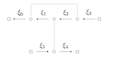
Figure 1: Graph with $n=3$ and $m=1$ corresponding to the pairs $(\xi_{1},\xi_{3})$ and $(\xi_{2},\xi_{5})$ and the delta functions $\delta(\xi_{1}-\xi_{0}+\xi_{3}-\xi_{2})$ and $\delta(\xi_{2}-\xi_{1}+\xi_{5}-\xi_{4})$.

The collection of pairs $(\xi_{k},\xi_{l(k)})$ for ${\bar{n}}$ values of $k$ and ${\bar{n}}$ values of $l(k)$ constitutes a graph $\mathfrak{g}\in\mathfrak{G}$ constructed as follows; see Fig.1 and [5]. The upper part of the graph with $n$ bullets represents $\hat{u}_{\varepsilon,n}$ while the lower part with $m$ bullets represents $\overline{\hat{u}_{\varepsilon,m}}$. The two squares on the left of the graph represent the variables $\xi_{0}$ and $\xi_{n+m+1}$ in $U_{\varepsilon}^{n,m}(t,\xi_{0},\xi_{n+m+1})$ while the squares on the right represent $\hat{u}_{0}(\xi_{n})$ and $\bar{\hat{u}}_{0}(\xi_{n+1})$. The dotted pairing lines represent the pairs of the graph $\mathfrak{g}$. Here, $\mathfrak{G}$ denotes the collection of all possible $|\mathfrak{G}|=\frac{(2{\bar{n}}-1)!}{2^{{\bar{n}}-1}({\bar{n}}-1)!}$ graphs that can be constructed for a given ${\bar{n}}$.

We denote by $A_{0}=A_{0}(\mathfrak{g})$ the collection of the ${\bar{n}}$ values of $k$ and by $B_{0}=B_{0}(\mathfrak{g})$ the collection of the ${\bar{n}}$ values of $l(k)$. We then find that

$$\mathbb{E}\Big{\{}\prod_{k=0,k\not=n}^{n+m}\hat{q}_{\varepsilon}(\xi_{k}-\xi_{k-1})\Big{\}}=\displaystyle\sum_{\mathfrak{g}\in\mathfrak{G}}\displaystyle\prod_{k\in A_{0}(\mathfrak{g})}\varepsilon^{d-2\alpha}\hat{R}(\varepsilon(\xi_{k}-\xi_{k-1}))\delta(\xi_{k}-\xi_{k-1}+\xi_{l(k)}-\xi_{l(k)-1}).$$

This provides us with an explicit expression for $U_{\varepsilon}^{n,m}(t,\xi_{0},\xi_{n+m+1})$ as a summation over all possible graphs generated by moments of Gaussian random variables. We need to introduce several classes of graphs.

We say that the graph has a crossing if there is a $k\leq n$ such that $l(k)\geq n+2$. We denote by $\mathfrak{G}_{c}\subset\mathfrak{G}$ the set of graphs with at least one crossing and by $\mathfrak{G}_{nc}=\mathfrak{G}\backslash\mathfrak{G}_{c}$ the non-crossing graphs. We observe that $V^{n,m}_{\varepsilon}(t,\xi_{0},\xi_{n+m+1})$ is the sum over the crossing graphs and that $U_{\varepsilon}^{n}(t,\xi_{0})\overline{U_{\varepsilon}^{m}(t,\xi_{n+m+1})}$ is the sum over the non-crossing graphs in $U^{n,m}_{\varepsilon}(t,\xi_{0},\xi_{n+m+1})$.

The unique graph $\mathfrak{g}_{s}$ with only simple pairs is called the simple graph and we define $\mathfrak{G}_{ns}=\mathfrak{G}\backslash\mathfrak{g}_{s}$. We denote by $\mathfrak{G}_{cs}$ the crossing simple graphs with only simple pairs except for exactly one crossing. The complement of $\mathfrak{G}_{cs}$ in the crossing graphs is denoted by $\mathfrak{G}_{cns}=\mathfrak{G}_{c}\backslash\mathfrak{G}_{cs}$.

As we shall see, only the simple graph $\mathfrak{g}_{s}$ contributes an $O(1)$ term in the limit $\varepsilon\to 0$ and only the graphs in $\mathfrak{G}_{cs}$ contribute to the leading order $O(\varepsilon^{\frac{1}{2}(d-2\alpha)})$ in the fluctuations of $\hat{u}_{\varepsilon}$.

The graphs are defined similarly in the calculation of $U_{\varepsilon}^{n}(t,\xi_{0})$ in (18) for $n=2{\bar{n}}$ and $m=0$, except that crossing graphs have no meaning in such a context. A summation over $k\in A_{0}(\mathfrak{g})$ of all the arguments $\xi_{k}-\xi_{k-1}+\xi_{l(k)}-\xi_{l(k)-1}$ of the $\delta$ functions shows that the last delta function may be replaced without modifying the integral in $U_{\varepsilon}^{n}(t,\xi_{0})$ by $\delta(\xi_{0}-\xi_{n})$.

This allows us to summarize the above calculations as follows:

$$\begin{array}[]{l}U_{\varepsilon}^{n,m}(t,\xi_{0},\xi_{n+m+1})=\displaystyle\int\prod_{k=0}^{n+m+1}e^{-s_{k}\xi_{k}^{\mathfrak{m}}}\hat{u}_{0}(\xi_{n})\bar{\hat{u}}_{0}(\xi_{n+1})\displaystyle\sum_{\mathfrak{g}\in\mathfrak{G}}\\ \qquad\displaystyle\prod_{k\in A_{0}(\mathfrak{g})}\varepsilon^{d-2\alpha}\hat{R}(\varepsilon(\xi_{k}-\xi_{k-1}))\delta(\xi_{k}-\xi_{k-1}+\xi_{l(k)}-\xi_{l(k)-1})d\mathbf{s}d\boldsymbol{\xi}.\end{array}$$ (22)

Similarly,

$$\begin{array}[]{l}U_{\varepsilon}^{n}(t,\xi_{0})=\hat{u}_{0}(\xi_{0})\displaystyle\int\prod_{k=0}^{n}e^{-s_{k}\xi_{k}^{\mathfrak{m}}}\displaystyle\sum_{\mathfrak{g}\in\mathfrak{G}}\\ \qquad\displaystyle\prod_{k\in A_{0}(\mathfrak{g})}\varepsilon^{d-2\alpha}\hat{R}(\varepsilon(\xi_{k}-\xi_{k-1}))\delta(\xi_{k}-\xi_{k-1}+\xi_{l(k)}-\xi_{l(k)-1})d\mathbf{s}d\boldsymbol{\xi}.\!\!\!\!\!\!\!\!\!\!\!\!\end{array}$$ (23)

2.3 Analysis of crossing graphs

We now analyze the influence of the crossing graphs on $I_{\varepsilon}(t)$ and $X_{\varepsilon}(t)$ defined in (20) and (21), respectively, for sufficiently small times. We obtain from (19) and (22) that

$$\begin{array}[]{l}V^{n,m}_{\varepsilon}(t,\xi_{0},\xi_{n+m+1})=\displaystyle\sum_{\mathfrak{g}\in\mathfrak{G}_{c}}\displaystyle\int\prod_{k=0}^{n+m+1}e^{-s_{k}\xi_{k}^{\mathfrak{m}}}\hat{u}_{0}(\xi_{n})\bar{\hat{u}}_{0}(\xi_{n+1})\\ \qquad\quad\displaystyle\prod_{k\in A_{0}(\mathfrak{g})}\varepsilon^{d-2\alpha}\hat{R}(\varepsilon(\xi_{k}-\xi_{k-1}))\delta(\xi_{k}-\xi_{k-1}+\xi_{l(k)}-\xi_{l(k)-1})\,d\mathbf{s}\,d\boldsymbol{\xi},\end{array}$$ (24)

involves the summation over the crossing graphs $\mathfrak{G}_{c}$. Let us consider a graph $\mathfrak{g}\in\mathfrak{G}_{c}$ with $M$ crossing pairs, $M\geq 1$. Crossing pairs are defined by $k\leq n$ and $l(k)\geq n+2$. Denote by $(\xi_{q_{m}},\xi_{l(q_{m})})$, $1\leq m\leq M$ the crossing pairs and define $Q=\max_{m}\{q_{m}\}$. By summing the arguments inside the delta functions for all $k\leq n$, we observe that the last of these delta functions may be replaced by

$$\delta(\xi_{0}-\xi_{n}+\displaystyle\sum_{m=1}^{M}\xi_{q_{m}}-\xi_{q_{m}-1}).$$

Similarly, by summing over all pairs with $k\geq n+2$, we obtain that the last of these delta functions may be replaced by

$$\delta(\xi_{n+1}-\xi_{n+m+1}+\displaystyle\sum_{m=1}^{M}\xi_{l(q_{m})}-\xi_{l(q_{m})-1}).$$

The product of the latter two delta functions is then equivalent to

$$\delta(\xi_{n+m+1}-\xi_{n+1}+\xi_{n}-\xi_{0})\delta(\xi_{Q}-\xi_{Q-1}+\xi_{0}-\xi_{n}+\displaystyle\sum_{m=1}^{M-1}\xi_{q_{m}}-\xi_{q_{m}-1}).$$

The analysis of the contributions of the crossing graphs is slightly different for the energy in (20) and for the spatial moments in (21). We start with the energy.

Analysis of the crossing terms in $I_{\varepsilon}(t)$.

We evaluate the expression for $|V^{n,m}_{\varepsilon}(t,\xi_{0},\xi_{0})|$ in (24) at $\xi_{n+m+1}=\xi_{0}$ and integrate in the $\xi_{0}$ variable over $\mathbb{R}^{d}$. Let us define $A^{\prime}=A_{0}\backslash\{Q\}$. For each $k\in A^{\prime}\cup\{0\}$, we perform the change of variables $\xi_{k}\to\frac{\xi_{k}}{\varepsilon}$. We then define

$$\xi_{k}^{\varepsilon}=\left\{\begin{array}[]{ll}\xi_{k}&k\not\in A^{\prime}\cup\{0\}\\ \frac{\xi_{k}}{\varepsilon}&k\in A^{\prime}\cup\{0\}.\end{array}\right.$$ (25)

Note that $\xi_{n}=\xi_{n+1}$ since $\xi_{n+m+1}=\xi_{0}$. This allows us to obtain that

$$\begin{array}[]{l}\displaystyle\int_{\mathbb{R}^{d}}|V_{\varepsilon}^{n,m}(t,\xi_{0},\xi_{0})|d\xi_{0}\leq\displaystyle\sum_{\mathfrak{g}\in\mathfrak{G}_{c}}\displaystyle\int e^{-(s_{0}+s_{n+m+1})\varepsilon^{-{\mathfrak{m}}}\xi_{0}^{\mathfrak{m}}}\prod_{k=1}^{n+m}e^{-s_{k}(\xi_{k}^{\varepsilon})^{\mathfrak{m}}}|\hat{u}_{0}(\xi_{n})|^{2}\\ \qquad\displaystyle\prod_{k\in A^{\prime}(\mathfrak{g})}\varepsilon^{-2\alpha}\hat{R}(\xi_{k}-\varepsilon\xi^{\varepsilon}_{k-1})\delta(\frac{\xi_{k}}{\varepsilon}-\xi^{\varepsilon}_{k-1}+\xi_{l(k)}-\xi^{\varepsilon}_{l(k)-1})\\ \qquad\varepsilon^{-2\alpha}\hat{R}(\xi_{0}-\varepsilon\xi_{n}+\displaystyle\sum_{m=1}^{M}\xi_{q_{m}}-\varepsilon\xi^{\varepsilon}_{q_{m}-1})\delta(\xi_{n+1}-\xi_{n})d\mathbf{s}d\boldsymbol{\xi}.\end{array}$$ (26)

Here $d\boldsymbol{\xi}$ also includes the integration in the variable $\xi_{0}$. The estimates for $V^{n,m}_{\varepsilon}$ here and in subsequent sections rely on integrating selected time variables. All estimates are performed as the following lemma indicates.

Lemma 2.1

Let $t>0$ given and consider an integral of the form

$$I_{n-1}=\displaystyle\prod_{k=0}^{n-1}\displaystyle\int_{0}^{t_{k}(\mathbf{s})}\Big{(}\prod_{k=0}^{n-1}f_{k}(s_{k})\Big{)}\prod_{k=0}^{n-1}ds_{k},$$ (27)

where $0\leq f_{k}(\mathbf{s})\leq 1$ for $0\leq k\leq n$ and assume that $\int_{0}^{t}f_{n-1}(s_{n-1})ds_{n-1}\leq h\wedge t$. Then

$$I_{n-2}\leq(h\wedge t)I_{n-1}.$$ (28)

Moreover, let ${\mathfrak{s}}$ be a permutation of the indices $0\leq k\leq n-1$. Define $I^{\mathfrak{s}}_{n-1}$ as $I_{n-1}$ with $f_{k}$ replaced by $f_{{\mathfrak{s}}(k)}$. Then $I^{\mathfrak{s}}_{n-1}=I_{n-1}$.

Using the above result with the permutation leaving all indices fixed except ${\mathfrak{s}}(n-1)=K$ and ${\mathfrak{s}}(K)=n-1$ for some $0\leq K\leq n-2$ allows us to estimate $I_{n-1}$ by integrating in the $K$th variable.

Proof. The derivation of (28) is immediate. We also calculate

$$\begin{array}[]{rclrcl}I_{n-1}&=&\displaystyle\int_{\mathbb{R}_{+}^{n+1}}\Big{(}\prod_{k=0}^{n-1}f_{k}(s_{k})\Big{)}\delta\big{(}t-\displaystyle\sum_{k=0}^{n}s_{k}\big{)}\prod_{k=0}^{n}ds_{k}\\ &=&\displaystyle\int_{\mathbb{R}_{+}^{n+1}}\Big{(}\prod_{k=0}^{n-1}f_{{\mathfrak{s}}(k)}(s_{{\mathfrak{s}}(k)})\Big{)}\delta\big{(}t-\displaystyle\sum_{k=0}^{n}s_{{\mathfrak{s}}(k)}\big{)}\prod_{k=0}^{n}ds_{k}\\ &=&\displaystyle\int_{\mathbb{R}_{+}^{n+1}}\Big{(}\prod_{k=0}^{n-1}f_{{\mathfrak{s}}(k)}(s_{k})\Big{)}\delta\big{(}t-\displaystyle\sum_{k=0}^{n}s_{k}\big{)}\prod_{k=0}^{n}ds_{k}&=&I^{\mathfrak{s}}_{n-1}.\end{array}$$

     

Note that $e^{-s_{n}(\mathbf{s})(\xi_{\varepsilon}^{n})^{\mathfrak{m}}}$ and $e^{-s_{n+1}(\mathbf{s})(\xi_{\varepsilon}^{n+1})^{\mathfrak{m}}}$ are bounded by $1$. We now estimate the integrals in the variables $s_{0}$, $s_{n+m+1}$, and $s_{k}$ for $k\in A^{\prime}$ in (26). Note that $n+1$ cannot belong to $A^{\prime}$ and that $n$ does not belong to $A^{\prime}$ either since either $n=Q$ (last crossing) or $n\in B_{0}$ is a receiving end of the pairing line $k\to l(k)$. Each integral is bounded by:

$$\int_{0}^{\tau\wedge t}e^{-s\varepsilon^{-{\mathfrak{m}}}\xi^{\mathfrak{m}}}ds\leq\dfrac{\varepsilon^{\mathfrak{m}}}{\xi^{\mathfrak{m}}}\wedge t.$$ (29)

The remaining exponential terms $e^{-s_{k}(\xi^{\varepsilon}_{k})^{\mathfrak{m}}}$ are bounded by $1$. Using lemma 2.1, this allows us to obtain that

$$\begin{array}[]{l}\displaystyle\int_{\mathbb{R}^{d}}|V_{\varepsilon}^{n,m}(t,\xi_{0},\xi_{0})|d\xi_{0}\leq\displaystyle\sum_{\mathfrak{g}\in\mathfrak{G}_{c}}\Big{(}\displaystyle\int d\tilde{\mathbf{s}}\Big{)}\displaystyle\int|\hat{u}_{0}(\xi_{n})|^{2}\\ \qquad\displaystyle\prod_{k\in A^{\prime}(\mathfrak{g})}\varepsilon^{-2\alpha}\Big{(}\dfrac{\varepsilon^{{\mathfrak{m}}}}{\xi_{k}^{\mathfrak{m}}}\wedge t\Big{)}\hat{R}(\xi_{k}-\varepsilon\xi^{\varepsilon}_{k-1})\delta(\frac{\xi_{k}}{\varepsilon}-\xi^{\varepsilon}_{k-1}+\xi_{l(k)}-\xi^{\varepsilon}_{l(k)-1})\\ \qquad\varepsilon^{-2\alpha}\Big{(}\dfrac{\varepsilon^{{\mathfrak{m}}}}{\xi_{0}^{\mathfrak{m}}}\wedge t\Big{)}^{2}\hat{R}(\xi_{0}-\varepsilon\xi_{n}+\displaystyle\sum_{m=1}^{M}\xi_{q_{m}}-\varepsilon\xi^{\varepsilon}_{q_{m}-1})\delta(\xi_{n+1}-\xi_{n})\,d\boldsymbol{\xi}.\end{array}$$

Here, $d\tilde{\mathbf{s}}$ corresponds to the integration in the remaining time variables $s_{k}$ for $k\not\in A^{\prime}\cup\{n+m+1\}$. There are $2{\bar{n}}-1-({\bar{n}}+1)={\bar{n}}-2$ such variables. Note the square on the last line, which comes from integrating in both variables $s_{0}$ and $s_{n+m+1}$.

The delta functions allow us to integrate in the variables $\xi_{l(k)}$ for $k\in A^{\prime}(\mathfrak{g})$ and the initial condition $\hat{u}_{0}(\xi_{n})$ in the variable $\xi_{n}$. Thanks to lemma 2.2 below, the power spectra allow us to integrate in the remaining variables in $A^{\prime}\cup\{0\}$. The integrals in the variables in $A^{\prime}$ are all bounded by $\rho_{f}$ defined in lemma 2.2 whereas the integral in $\xi_{0}$ results in a bound equal to $\varepsilon^{\beta}\rho_{f}$, where $\varepsilon^{\beta}$ is defined in (6). As a consequence, we have the bound

$$\int_{\mathbb{R}^{d}}|V_{\varepsilon}^{n,m}(t,\xi_{0},\xi_{0})|d\xi_{0}\leq\displaystyle\sum_{\mathfrak{g}\in\mathfrak{G}_{c}}\Big{(}\displaystyle\int d\tilde{\mathbf{s}}\Big{)}\rho_{f}^{{\bar{n}}-1}\|\hat{u}_{0}\|^{2}\rho_{f}\varepsilon^{\beta}=\displaystyle\sum_{\mathfrak{g}\in\mathfrak{G}_{c}}\Big{(}\displaystyle\int d\tilde{\mathbf{s}}\Big{)}\rho_{f}^{{\bar{n}}}\varepsilon^{\beta}\|\hat{u}_{0}\|^{2}.$$

Using Stirling’s formula, we find that $|\mathfrak{G}_{c}|<\frac{(2{\bar{n}}-1)!}{2^{{\bar{n}}-1}({\bar{n}}-1)!}$ is bounded by $(\frac{2{\bar{n}}}{e})^{{\bar{n}}}$. It remains to evaluate the integrals in time. We verify that

$$\prod_{k=0}^{n-1}\displaystyle\int_{0}^{t_{k}(\mathbf{s})}ds_{0}\cdots ds_{n-1}=\dfrac{t^{n}}{n!},\qquad t_{k}(\mathbf{s})=t-s_{0}-\ldots-s_{k-1}.$$ (30)

Let $\bar{p}=\bar{p}(\mathfrak{g})$ be the number of $s_{k}$ for $k\leq n$ in $\tilde{\mathbf{s}}$ and $\bar{q}=\bar{q}(\mathfrak{g})$ be the number of $s_{k}$ for $k\geq n+1$ in $\tilde{\mathbf{s}}$, with $\bar{p}+\bar{q}={\bar{n}}-1$. Using (30), we thus find that

$$\Big{(}\displaystyle\int d\tilde{\mathbf{s}}\Big{)}=\dfrac{t^{\bar{p}}}{\bar{p}!}\dfrac{t^{\bar{q}}}{\bar{q}!}=\dfrac{t^{{\bar{n}}-1}}{({\bar{n}}-1)!}{{\bar{n}}-1\choose\bar{p}}\leq t^{{\bar{n}}-1}\Big{(}\dfrac{{\bar{n}}-1}{2e}\Big{)}^{-{\bar{n}}+1}\leq t^{{\bar{n}}-1}{\bar{n}}\Big{(}\dfrac{{\bar{n}}}{2e}\Big{)}^{-{\bar{n}}}$$

using Stirling’s formula. This shows that

$$\sum_{\mathfrak{g}\in\mathfrak{G}_{c}}\Big{(}\displaystyle\int d\tilde{\mathbf{s}}\Big{)}\leq\dfrac{{\bar{n}}}{T}(4\rho_{f}T)^{\bar{n}},$$ (31)

uniformly for $t\in(0,T)$. We thus need to choose $T$ sufficiently small so that $4\rho_{f}T<1$. Then, for ${\mathfrak{r}}$ such that $4\rho_{f}T<{\mathfrak{r}}^{2}<1$, we find that

$$\int|V_{\varepsilon}^{n,m}(t,\xi_{0},\xi_{0})|d\xi_{0}\leq C{\mathfrak{r}}^{n+m}\varepsilon^{\beta}\|\hat{u}_{0}\|^{2},$$ (32)

for some positive constant $C$. It remains to sum over $n$ and $m$ to obtain that

$$\big{|}\mathbb{E}\{I_{\varepsilon}(t)\}-\displaystyle\int_{\mathbb{R}^{d}}\mathbb{E}\{\hat{u}_{\varepsilon}(t,\xi)\}^{2}d\xi\big{|}\leq\dfrac{C}{{\mathfrak{r}}^{2}}\varepsilon^{\beta}\|\hat{u}_{0}\|^{2}.$$ (33)

We shall analyze the non-crossing terms generating $|\mathbb{E}\{\hat{u}_{\varepsilon}(t,\xi)\}|^{2}$ shortly. Before doing so, we analyze the influence of the crossing terms on $X_{\varepsilon}$. We can verify that the error term $\varepsilon^{\beta}$ in (33) is optimal, for instance by looking at the contribution of the graph with $n=m=1$.

Analysis of the crossing terms in $X_{\varepsilon}$.

It turns out that the contribution of the crossing terms is smaller for the moment $X_{\varepsilon}$ than it is for the energy $I_{\varepsilon}$. More precisely, we show that the smallest contribution to the variance of $X_{\varepsilon}$ is of order $\varepsilon^{d-2\alpha}$ for graphs in $\mathfrak{G}_{cs}$ and of order $\varepsilon^{d-2\alpha+\beta}$ for the other crossing graphs.

We come back to (24) and this time perform the change of variables $\xi_{k}\to\frac{\xi_{k}}{\varepsilon}$ for $k\in A^{\prime}$ only. We re-define

$$\xi_{k}^{\varepsilon}=\left\{\begin{array}[]{ll}\xi_{k}&k\not\in A^{\prime}\\ \frac{\xi_{k}}{\varepsilon}&k\in A^{\prime},\end{array}\right.$$ (34)

and find that

$$\begin{array}[]{l}V_{\varepsilon}^{n,m}(t,\xi_{0},\xi_{n+m+1})=\displaystyle\sum_{\mathfrak{g}\in\mathfrak{G}_{c}}\displaystyle\int\prod_{k=0}^{n+m+1}e^{-s_{k}(\xi_{k}^{\varepsilon})^{\mathfrak{m}}}\hat{u}_{0}(\xi_{n})\bar{\hat{u}}_{0}(\xi_{n+1})\\ \qquad\displaystyle\prod_{k\in A^{\prime}(\mathfrak{g})}\varepsilon^{-2\alpha}\hat{R}(\xi_{k}-\varepsilon\xi^{\varepsilon}_{k-1})\delta(\frac{\xi_{k}}{\varepsilon}-\xi^{\varepsilon}_{k-1}+\xi_{l(k)}-\xi^{\varepsilon}_{l(k)-1})\\ \qquad\varepsilon^{d-2\alpha}\hat{R}(\varepsilon(\xi_{Q}-\xi^{\varepsilon}_{Q-1}))\delta(\xi_{n+m+1}-\xi_{n+1}+\xi_{n}-\xi_{0})d\mathbf{s}d\boldsymbol{\xi}.\end{array}$$ (35)

Note that neither $n$ nor $n+m+1$ belong to $A^{\prime}(\mathfrak{g})$. For each $k\in A^{\prime}(\mathfrak{g})$, we integrate in $s_{k}$ and obtain using (29) that

$$\begin{array}[]{l}|V_{\varepsilon}^{n,m}(t,\xi_{0},\xi_{n+m+1})|\leq\displaystyle\sum_{\mathfrak{g}\in\mathfrak{G}_{c}}\displaystyle\int\displaystyle\prod_{k\not\in A^{\prime}(\mathfrak{g})}e^{-s_{k}\xi_{k}^{\mathfrak{m}}}|\hat{u}_{0}(\xi_{n})\bar{\hat{u}}_{0}(\xi_{n+1})|\\ \qquad\displaystyle\prod_{k\in A^{\prime}(\mathfrak{g})}\varepsilon^{-2\alpha}\Big{(}\dfrac{\varepsilon^{\mathfrak{m}}}{\xi_{k}^{\mathfrak{m}}}\wedge t\Big{)}\hat{R}(\xi_{k}-\varepsilon\xi^{\varepsilon}_{k-1})\delta(\frac{\xi_{k}}{\varepsilon}-\xi^{\varepsilon}_{k-1}+\xi_{l(k)}-\xi^{\varepsilon}_{l(k)-1})\\ \qquad\varepsilon^{d-2\alpha}\hat{R}(\varepsilon(\xi_{Q}-\xi^{\varepsilon}_{Q-1}))\delta(\xi_{n+m+1}-\xi_{n+1}+\xi_{n}-\xi_{0})d\tilde{\mathbf{s}}d\boldsymbol{\xi}.\end{array}$$ (36)

By assumption on $\hat{R}(\xi)$, we know the existence of a constant $\hat{R}_{\infty}$ such that

$$\varepsilon^{d-2\alpha}\hat{R}(\varepsilon(\xi_{Q}-\xi^{\varepsilon}_{Q-1}))\leq\varepsilon^{d-2\alpha}\hat{R}_{\infty}.$$ (37)

This is where the factor $\varepsilon^{d-2\alpha}$ arises. We need however to ensure that the integral in $\xi_{Q}$ is well-defined. We have two possible scenarios: either $Q=n$ or $n\in B_{0}$. When $Q=n$, the integration in $\xi_{Q}$ is an integration in $\xi_{n}$ for which we use $\hat{u}_{0}(\xi_{n})$. When $n\in B_{0}$, we thus have $n=l(k_{0})$ for some $k_{0}$ and we replace the delta function involving $\xi_{n}$ by a delta function involving $\xi_{Q}$ given equivalently by

$$\delta(\xi_{Q}-\xi_{Q-1}+\xi_{0}-\xi_{n}+\displaystyle\sum_{m=1}^{M}\xi_{q_{m}}-\xi_{q_{m}-1}).$$ (38)

In either scenario, we can integrate in the variable $\xi_{Q}$ without using the term $\hat{R}(\varepsilon(\xi_{Q}-\xi_{Q-1}))$. We use the inequality

$$|\hat{u}_{0}(\xi_{n})\bar{\hat{u}}_{0}(\xi_{n+1})|\leq\dfrac{1}{2}\Big{(}|\hat{u}_{0}(\xi_{n})|^{2}+|\hat{u}_{0}(\xi_{n}-\xi_{0}+\xi_{n+m+1})|^{2}\Big{)},$$ (39)

to obtain the bound

$$|V_{\varepsilon}^{n,m}(t,\xi_{0},\xi_{n+m+1})|\leq\varepsilon^{d-2\alpha}\hat{R}_{\infty}\displaystyle\sum_{\mathfrak{g}\in\mathfrak{G}_{c}}\Big{(}\displaystyle\int d\tilde{s}\Big{)}\rho_{f}^{{\bar{n}}-1}\|\hat{u}_{0}\|^{2}.$$ (40)

The bound is uniform in $\xi_{0}$ and $\xi_{n+m+1}$. Using (31) and (32), we obtain

$$|V_{\varepsilon}^{n,m}(t,\xi_{0},\xi_{n+m+1})|\leq\varepsilon^{d-2\alpha}{\mathfrak{r}}^{n+m}\|\hat{u}_{0}\|^{2}.$$ (41)

After summation in $n,m\in\mathbb{N}$, we thus find that

$$\mathbb{E}\{(X_{\varepsilon}-\mathbb{E}\{X_{\varepsilon}\})^{2}\}\leq\dfrac{C}{{\mathfrak{r}}^{2}}\varepsilon^{d-2\alpha}\|\hat{u}_{0}\|^{2}\|\hat{M}\|_{1}^{2}.$$ (42)

Similarly, by setting $\xi_{n+m+1}=\xi_{0}$, we find that

$$\Big{|}\mathbb{E}\Big{\{}\displaystyle\int_{\mathbb{R}^{d}}|\hat{u}_{\varepsilon}|^{2}(t,\xi)\varphi(\xi)d\xi\Big{\}}-\displaystyle\int_{\mathbb{R}^{d}}|\mathbb{E}\{\hat{u}_{\varepsilon}(t,\xi)\}|^{2}\varphi(\xi)d\xi\Big{|}\leq\dfrac{C}{{\mathfrak{r}}^{2}}\varepsilon^{d-2\alpha}\|\hat{u}_{0}\|^{2}\|\varphi\|_{1},$$ (43)

for any test function $\varphi\in L^{1}(\mathbb{R}^{d})$. This local energy estimate is to be compared with the global estimate obtained in (33).

Analysis of the leading crossing terms in $X_{\varepsilon}$.

The preceding estimate on $X_{\varepsilon}$ may be refined as only the crossing graphs in $\mathfrak{G}_{cs}$ have contributions of order $\varepsilon^{d-2\alpha}$. We return to the bound (36) and obtain that

$$\begin{array}[]{l}|V_{\varepsilon}^{n,m}(t,\xi_{0},\xi_{n+m+1})|\leq\varepsilon^{d-2\alpha}\hat{R}_{\infty}\displaystyle\sum_{\mathfrak{g}\in\mathfrak{G}_{c}}\displaystyle\int\displaystyle\prod_{k\not\in A^{\prime}(\mathfrak{g})}e^{-s_{k}(\xi_{k})^{\mathfrak{m}}}|\hat{u}_{0}(\xi_{n})\bar{\hat{u}}_{0}(\xi_{n+1})|\\ \qquad\displaystyle\prod_{k\in A^{\prime}(\mathfrak{g})}\varepsilon^{-2\alpha}\Big{(}\dfrac{\varepsilon^{\mathfrak{m}}}{\xi_{k}^{\mathfrak{m}}}\wedge t\Big{)}\hat{R}(\xi_{k}-\varepsilon\xi^{\varepsilon}_{k-1})\delta(\frac{\xi_{k}}{\varepsilon}-\xi^{\varepsilon}_{k-1}+\xi_{l(k)}-\xi^{\varepsilon}_{l(k)-1})\\ \qquad\delta(\xi_{n+m+1}-\xi_{n+1}+\xi_{n}-\xi_{0})d\tilde{\mathbf{s}}d\boldsymbol{\xi}.\end{array}$$ (44)

The ${\bar{n}}+3$ variables in time left are $s_{0}$, $s_{n+1}$, $s_{Q}$, $s_{l(Q)}$, and the ${\bar{n}}-1$ variables $s_{l(A^{\prime}(\mathfrak{g}))}$.

Let $\mathfrak{g}\in\mathfrak{G}_{c}$. Let us assume that for some $k$ such that $(\xi_{k},\xi_{l(k)})$ is not a crossing pair, we have $l(k)-1>k$, i.e., $\mathfrak{g}\in\mathfrak{G}_{ncs}$. The non-crossing pairs are not affected by the possible change of a delta function involving $\xi_{n}$ to a delta function involving $\xi_{Q}$. We may then integrate in the variable $s_{l(k)}$ and obtain the bound for the integral

$$\begin{array}[]{ll}\varepsilon^{d-2\alpha}\hat{R}_{\infty}\displaystyle\int d\tilde{\mathbf{s}}d\boldsymbol{\xi}|\hat{u}_{0}(\xi_{n})\bar{\hat{u}}_{0}(\xi_{n+1})|\delta(\xi_{n+m+1}-\xi_{n+1}+\xi_{n}-\xi_{0})\\[8.53581pt] \displaystyle\prod_{k\in A^{\prime}(\mathfrak{g})}\Big{(}\dfrac{\varepsilon^{\mathfrak{m}}}{\xi_{k}^{\mathfrak{m}}}\wedge t\Big{)}\Big{(}\dfrac{\varepsilon^{\mathfrak{m}}}{|\xi_{k}-\varepsilon\xi_{k-1}^{\varepsilon}-\varepsilon\xi_{l(k)-1}^{\varepsilon}|^{\mathfrak{m}}}\wedge t\Big{)}\hat{R}(\xi_{k}-\varepsilon\xi^{\varepsilon}_{k-1})\delta(\frac{\xi_{k}}{\varepsilon}-\xi^{\varepsilon}_{k-1}+\xi_{l(k)}-\xi^{\varepsilon}_{l(k)-1})\\ \leq\varepsilon^{\beta}\varepsilon^{d-2\alpha}\Big{(}\displaystyle\int d\tilde{\mathbf{s}}\Big{)}\hat{R}_{\infty}\rho_{f}^{{\bar{n}}-1}\|\hat{u}_{0}\|^{2},\end{array}$$

thanks to lemma 2.2 below. The summation over all graphs in $\mathfrak{G}_{ncs}$ of any quantity derived from $V_{\varepsilon}^{n,m}(t,\xi_{0},\xi_{n+m+1})$ is therefore $\varepsilon^{\beta}$ smaller than the corresponding sum over all graphs in $\mathfrak{G}_{c}$. We thus see that any non-crossing pair has to be of the form $l(k)-1=k$, i.e., a simple pair, in order for the graph to correspond to a contribution of order $\varepsilon^{d-2\alpha}$.

Let us consider the graphs composed of crossings and simple pairs. We may delete the simple pairs from the graph since they contribute integrals of order $O(1)$ thanks to lemma 2.2 below and assume that the graph is composed of crossings only, thus with $n=m$ and $Q=n$ after deletion of the simple pairs. Let us consider $k<n$ with $l(k)\geq n+1$ so that the delta function

$$\delta(\dfrac{\xi_{k}}{\varepsilon}-\xi_{k-1}^{\varepsilon}+\xi_{l(k)}-\xi_{l(k)-1})$$

is present in the integral defining $V^{n,m}_{\varepsilon}$. We find for the same reason as above that the contribution of the corresponding graph is of order $\varepsilon^{d-2\alpha}\varepsilon^{\beta}$ by integration in the variable $s_{l(k)}$. As a consequence, the only graph composed exclusively of crossing pairs that generates a contribution of order $\varepsilon^{d-2\alpha}$ is the graph with $n=m=1$. This concludes our proof that the contribution of order $\varepsilon^{d-2\alpha}$ in $V^{n,m}_{\varepsilon}$ is given by the $nm$ graphs in $\mathfrak{G}_{cs}$ when both $n$ and $m$ are even numbers (otherwise, $\mathfrak{G}_{cs}$ is empty). All other graphs in $\mathfrak{G}_{c}$ provide a contribution of order $\varepsilon^{\beta}$ smaller than what we obtained in (41). In other words, let us define

$$\begin{array}[]{l}V_{\varepsilon,s}^{n,m}(t,\xi_{0},\xi_{n+m+1})=\displaystyle\sum_{\mathfrak{g}\in\mathfrak{G}_{cs}}\displaystyle\int\prod_{k=0}^{n+m+1}e^{-s_{k}\xi_{k}^{\mathfrak{m}}}\hat{u}_{0}(\xi_{n})\bar{\hat{u}}_{0}(\xi_{n+1})\\ \qquad\displaystyle\prod_{k\in A_{0}(\mathfrak{g})}\varepsilon^{d-2\alpha}\hat{R}(\varepsilon(\xi_{k}-\xi_{k-1}))\delta(\xi_{k}-\xi_{k-1}+\xi_{l(k)}-\xi_{l(k)-1})d\mathbf{s}d\boldsymbol{\xi}.\end{array}$$ (45)

We have found that

$$|V_{\varepsilon}^{n,m}(t,\xi_{0},\xi_{n+m+1})-V_{\varepsilon,s}^{n,m}(t,\xi_{0},\xi_{n+m+1})|\lesssim\varepsilon^{d-2\alpha+\beta}{\mathfrak{r}}^{n+m}\|\hat{u}_{0}\|^{2}.$$ (46)

2.4 Analysis of non-crossing graphs

We now apply the estimates obtained in the preceding section to the analysis of the moments $U_{\varepsilon}^{n}(t)$ defined in (18) and given more explicitly in (23). Our objective is to show that only the simple graph $\mathfrak{g}$ contributes a term of order $O(1)$ in (23) whereas all other graphs in $\mathfrak{G}_{ns}$ contribute (summable in $n$) terms of order $O(\varepsilon^{\beta})$. Note that $n=2{\bar{n}}$, for otherwise, $U_{\varepsilon}^{n}(t)=0$. We recall that the simple graph is defined by $l(k)=k+1$. We thus define the simple graph contribution as

$$\begin{array}[]{rcl}U_{\varepsilon,s}^{n}(t,\xi_{0})&=&{\mathcal{U}}^{n}_{\varepsilon}(t,\xi_{0})\hat{u}_{0}(\xi_{0})\\ {\mathcal{U}}^{n}_{\varepsilon}(t,\xi_{0})&=&\displaystyle\int\prod_{k=0}^{n}e^{-s_{k}\xi_{k}^{\mathfrak{m}}}\prod_{k=0}^{{\bar{n}}-1}\varepsilon^{d-2\alpha}\hat{R}(\varepsilon(\xi_{2k+1}-\xi_{2k}))\delta(\xi_{2(k+1)}-\xi_{2k})d\mathbf{s}d\boldsymbol{\xi},\end{array}$$ (47)

and

$$U_{\varepsilon,s}(t,\xi_{0})=\displaystyle\sum_{n\in\mathbb{N}}U_{\varepsilon,s}^{n}(t,\xi_{0}):={\mathcal{U}}_{\varepsilon}(t,\xi_{0})\hat{u}_{0}(\xi_{0}).$$ (48)

For all $k\in A_{0}$, we perform the change of variables $\xi_{k}\to\frac{\xi_{k}}{\varepsilon}$ and (re-)define as before

$$\xi_{k}^{\varepsilon}=\left\{\begin{array}[]{ll}\xi_{k}&k\not\in A_{0}\\ \frac{\xi_{k}}{\varepsilon}&k\in A_{0}.\end{array}\right.$$ (49)

This gives

$$\begin{array}[]{l}U_{\varepsilon}^{n}(t,\xi_{0})=\hat{u}_{0}(\xi_{0})\displaystyle\sum_{\mathfrak{g}\in\mathfrak{G}}\displaystyle\int\prod_{k=0}^{n}e^{-s_{k}(\xi_{k}^{\varepsilon})^{\mathfrak{m}}}\\ \qquad\displaystyle\prod_{k\in A_{0}(\mathfrak{g})}\varepsilon^{-2\alpha}\hat{R}(\xi_{k}-\varepsilon\xi^{\varepsilon}_{k-1})\delta(\dfrac{\xi_{k}}{\varepsilon}-\xi^{\varepsilon}_{k-1}+\xi_{l(k)}-\xi^{\varepsilon}_{l(k)-1})d\mathbf{s}d\boldsymbol{\xi}.\end{array}$$ (50)

Assuming that $l(k)-1>k$ for one of the pairings, we obtain as in the analysis leading to (46) the following bound for the corresponding graph:

$$\begin{array}[]{l}|\hat{u}_{0}(\xi_{0})|\displaystyle\int d\tilde{\mathbf{s}}d\boldsymbol{\xi}\displaystyle\prod_{k\in A_{0}(\mathfrak{g})}\varepsilon^{-2\alpha}\Big{(}\dfrac{\varepsilon^{\mathfrak{m}}}{\xi_{k}^{\mathfrak{m}}}\wedge t\Big{)}\Big{(}\dfrac{\varepsilon^{\mathfrak{m}}}{|\xi_{k}-\varepsilon\xi_{k-1}^{\varepsilon}-\varepsilon\xi_{l(k)-1}^{\varepsilon}|^{\mathfrak{m}}}\wedge t\Big{)}\\ \qquad\qquad\hat{R}(\xi_{k}-\varepsilon\xi^{\varepsilon}_{k-1})\delta(\dfrac{\xi_{k}}{\varepsilon}-\xi^{\varepsilon}_{k-1}+\xi_{l(k)}-\xi^{\varepsilon}_{l(k)-1})\\[5.69054pt] \leq\varepsilon^{\beta}\Big{(}\displaystyle\int d\tilde{\mathbf{s}}\Big{)}\rho_{f}^{{\bar{n}}}|\hat{u}_{0}(\xi_{0})|.\end{array}$$

This shows that

$$|U_{\varepsilon}^{n}(t,\xi_{0})-U_{\varepsilon,s}^{n}(t,\xi_{0})|\leq|\hat{u}_{0}(\xi_{0})|\varepsilon^{\beta}{\mathfrak{r}}^{n},$$ (51)

so that

$$|\mathbb{E}\{\hat{u}_{\varepsilon}\}(t,\xi)-U_{\varepsilon,s}(t,\xi)|\lesssim\dfrac{1}{{\mathfrak{r}}}\varepsilon^{\beta}|\hat{u}_{0}(\xi)|,$$ (52)

at least for sufficiently small times $t\in(0,T)$ such that $4\rho_{f}T<1$. It remains to analyze the limit of $U_{\varepsilon,s}(t,\xi)$ to obtain the limiting behavior of $X_{\varepsilon}$ and $I_{\varepsilon,\varphi}$. This analysis is carried out in the next section. Another application of lemma 2.2 shows that $U_{\varepsilon,s}(t,\xi)$ is square integrable and that its $L^{2}(\mathbb{R}^{d})$ norm is bounded by $\|\hat{u}_{0}\|$. In other words, we have constructed a weak solution $\hat{u}_{\varepsilon}(t)\in L^{2}(\Omega\times\mathbb{R}^{d})$ to (13) since the series (15) converges uniformly in $L^{2}(\Omega\times\mathbb{R}^{d})$ for sufficiently small times $t\in(0,T)$ such that $4\rho_{f}T<1$.

Collecting the results obtained in (33) and (52), we have shown that

$$\begin{array}[]{rcl}\|(\hat{u}_{\varepsilon}-U_{\varepsilon,s})(t)\|_{L^{2}(\Omega\times\mathbb{R}^{d})}&\lesssim&\varepsilon^{\frac{\beta}{2}}\|\hat{u}_{0}\|_{L^{2}(\mathbb{R}^{d})},\end{array}$$

where $U_{\varepsilon,s}$ is the deterministic term given in (48). The analysis of $U_{\varepsilon,s}$ and that of $X_{\varepsilon}$ is postponed to section 3, after we state and prove lemma 2.2, which allows us to analyze the contributions of the different graphs.

Lemma 2.2

Let us assume that $\hat{R}$ is bounded by a smooth radially symmetric, decreasing function $f(r)$. We also assume that $f(r)\leq\tau_{f}r^{-{\mathfrak{n}}}$ for some $0\leq{\mathfrak{n}}<d-{\mathfrak{m}}$ in dimension $d>{\mathfrak{m}}$ and ${\mathfrak{n}}=0$ when $d\leq{\mathfrak{m}}$. Then we obtain the following estimates.
For $d>{\mathfrak{m}}$, we have

$$\int\dfrac{1}{|\xi_{k}|^{\mathfrak{m}}}\hat{R}(\xi_{k}-y)d\xi_{k}\leq\rho_{f}:=c_{d}\displaystyle\int_{0}^{\infty}\dfrac{1}{|\xi|^{\mathfrak{m}}}f(|\xi|)|\xi|^{d-1}d|\xi|\,\,\vee\,\,\tau_{f},$$

uniformly in $y\in\mathbb{R}^{d}$, where $c_{d}=|S^{d-1}|$ and $a\vee b=max(a,b)$. Moreover,

$$\int\dfrac{1}{|\xi_{k}|^{\mathfrak{m}}}\hat{R}(\xi_{k}-y)\Big{(}\dfrac{\varepsilon^{\mathfrak{m}}}{|\xi_{k}-z|^{\mathfrak{m}}}\wedge t\Big{)}d\xi_{k}\lesssim\,\rho_{f}\,\left\{\begin{array}[]{ll}\varepsilon^{{\mathfrak{m}}-{\mathfrak{n}}}&d>2{\mathfrak{m}}-{\mathfrak{n}}\\ \varepsilon^{{\mathfrak{m}}-{\mathfrak{n}}}|\ln\varepsilon|&d=2{\mathfrak{m}}-{\mathfrak{n}}\\ \varepsilon^{d-{\mathfrak{m}}-{\mathfrak{n}}}&{\mathfrak{m}}<d<2{\mathfrak{m}}-{\mathfrak{n}}.\end{array}\right.$$

For $d={\mathfrak{m}}$, we define $\rho_{f}=c_{d}f(0)$ and have

$$\int\Big{(}\dfrac{\varepsilon^{\mathfrak{m}}}{|\xi_{k}-z|^{\mathfrak{m}}}\wedge t\Big{)}^{l}\hat{R}(\xi_{k}-y)d\xi_{k}\lesssim\,\rho_{f}\,\left\{\begin{array}[]{ll}\varepsilon^{\mathfrak{m}}|\ln\varepsilon|&l=1\\ \varepsilon^{\mathfrak{m}}&l=2.\end{array}\right.$$

For $d<{\mathfrak{m}}$, we have

$$\int\Big{(}\dfrac{\varepsilon^{\mathfrak{m}}}{|\xi_{k}-z|^{\mathfrak{m}}}\wedge t\Big{)}^{l}\hat{R}(\xi_{k}-y)d\xi_{k}\lesssim\varepsilon^{d},\quad l\geq 1.$$

Proof. Once $\hat{R}$ is bounded above by a decreasing, radially symmetric, function $f(r)$, the above integrals are maximal when $y=z=0$ thanks to lemma 2.3 below since $|\xi|^{-{\mathfrak{m}}}$ and $(\varepsilon^{\mathfrak{m}}|\xi|^{-{\mathfrak{m}}}\wedge t)$ are radially symmetric and decreasing. The first bound is then obvious and defines $\rho_{f}$. The second bound is obvious in dimension $d>2{\mathfrak{m}}$ since $|\xi_{k}|^{-2{\mathfrak{m}}}$ is integrable.

All the bounds in the lemma are thus obtained from a bound for

$$\int_{0}^{\infty}\Big{(}\dfrac{\varepsilon^{\mathfrak{m}}}{r^{\mathfrak{m}}}\wedge t\Big{)}^{l}r^{d-1}f(r)dr.$$

We obtain that the above integral restricted to $r\in(1,\infty)$ is bounded by a constant times $\varepsilon^{{\mathfrak{m}}l}\rho_{f}$ for $d\geq{\mathfrak{m}}$ and by a constant times $\varepsilon^{{\mathfrak{m}}l}$ for $d<{\mathfrak{m}}$. It thus remains to bound the integral on $r\in(0,1)$, which is equal to

$$\int_{0}^{\varepsilon t^{-\frac{1}{{\mathfrak{m}}}}}t^{l}r^{d-1}f(r)dr+\displaystyle\int_{\varepsilon t^{-\frac{1}{{\mathfrak{m}}}}}^{1}\dfrac{\varepsilon^{l{\mathfrak{m}}}}{r^{l{\mathfrak{m}}}}r^{d-1}f(r)dr.$$

Replacing $f(r)$ by $\tau_{f}r^{-{\mathfrak{n}}}$, we find that the first integral is bounded by a constant times $\varepsilon^{d-{\mathfrak{n}}}$ and the second integral by a constant times $\varepsilon^{d-{\mathfrak{n}}}\vee\varepsilon^{l{\mathfrak{m}}}$ when $d-{\mathfrak{n}}-l{\mathfrak{m}}\not=0$ and $\varepsilon^{2{\mathfrak{m}}}|\ln\varepsilon|$ when $d=2{\mathfrak{m}}-{\mathfrak{n}}$. It remains to divide through by $\varepsilon^{\mathfrak{m}}$ when $l=2$ to obtain the desired results.        

Lemma 2.3

Let $f$, $g$, and $h$ be non negative, bounded, integrable, and radially symmetric functions on $\mathbb{R}^{d}$ that are decreasing as a function of radius. Then the integral

$$I_{\zeta,\tau}=\displaystyle\int_{\mathbb{R}^{d}}f(\xi-\zeta)g(\xi-\tau)h(\xi)d\xi,$$ (53)

which is well defined, is maximal at $\zeta=\tau=0$.

Proof. In a first step, we rotate $\zeta$ to align it with $\tau$. The first claim is that the integral cannot increase while doing so. Then we send $\zeta$ and $\tau$ to $0$. The second claim is that the integral again does not increase.

We assume that the functions $f$, $g$, and $h$ are smooth and obtain the result in the general case by density. We choose a system of coordinates so that $\tau=|\tau|e_{1}$, where $(e_{1},\ldots,e_{d})$ is an orthonormal basis of $\mathbb{R}^{d}$, and $\zeta=|\zeta|\hat{\theta}$ with $\hat{\theta}=(\cos\theta,\sin\theta,0,\ldots,0)$. Without loss of generality, we may assume that $\theta\in(0,\pi)$. Then $I_{\zeta,\tau}$ may be recast as $I_{\theta}$ and we find that

$$I_{\theta}=\displaystyle\int_{0}^{\infty}|\xi|^{d-1}h(|\xi|)J_{\theta}(|\xi|)d|\xi|,$$

where we denote $h(|\xi|)\equiv h(\xi)$ with the same convention for $f$ and $g$ and define

$$J_{\theta}(|\xi|)=\displaystyle\int_{S^{d-1}}f(|\xi|\psi-\zeta)g(|\xi|\psi-\tau)d\psi.$$

It is sufficient to show that $\partial_{\theta}J_{\theta}\leq 0$. We find

$$\partial_{\theta}J_{\theta}=\displaystyle\int_{S^{d-1}}-\hat{\theta}^{\perp}\cdot\nabla f(|\xi|\psi-\zeta)g(|\xi|\psi-\tau)d\psi,$$

with $\hat{\theta}^{\perp}=(-\sin\theta,\cos\theta,0,\ldots,0)$. We decompose the sphere as $\psi=(\psi\cdot\hat{\theta},\tilde{\psi})$ and find, for some positive weight $w(\mu)$ that

$$\begin{array}[]{rcl}\partial_{\theta}J_{\theta}&=&\displaystyle\int_{-1}^{1}d(\psi\cdot\hat{\theta})(-f^{\prime})(||\xi|\psi-\zeta|)w(\psi\cdot\hat{\theta})\displaystyle\int_{S^{d-2}}(\hat{\theta}^{\perp}\cdot\tilde{\psi})g(|\xi|\psi-\tau)d\tilde{\psi}.\end{array}$$

We now observe that

$$\begin{array}[]{rcl}&&\displaystyle\int_{S^{d-2}}(\hat{\theta}^{\perp}\cdot\tilde{\psi})g(|\xi|\psi-\tau)d\tilde{\psi}\\[8.53581pt] &=&\displaystyle\int_{\hat{\theta}^{\perp}\cdot\tilde{\psi}>0}(\hat{\theta}^{\perp}\cdot\tilde{\psi})\big{(}g(||\xi|(\hat{\theta}\cdot\psi\hat{\theta}+\tilde{\psi})-\tau|)-g(||\xi|(\hat{\theta}\cdot\psi\hat{\theta}-\tilde{\psi})-\tau|)\big{)}d\tilde{\psi}\,\leq\,0,\end{array}$$

as $||\xi|(\hat{\theta}\cdot\psi\hat{\theta}+\tilde{\psi})-\tau|\leq||\xi|(\hat{\theta}\cdot\psi\hat{\theta}-\tilde{\psi})-\tau|$ by construction. Indeed, we find that $||\xi|(\hat{\theta}\cdot\psi\hat{\theta}\pm\tilde{\psi})-\tau|^{2}-|\xi|^{2}-|\tau|^{2}+2|\tau||\xi|\hat{\theta}\cdot\psi\hat{\theta}\cdot\tau=\pm 2|\tau||\xi|\tilde{\psi}\cdot\tau=\pm 2|\tau||\xi|\hat{\theta}^{\perp}\cdot\tau$ whereas $\hat{\theta}^{\perp}\cdot\tau=-\sin\theta|\tau|<0$ by construction. This shows that $|\xi|(\hat{\theta}\cdot\psi\hat{\theta}+\tilde{\psi})$ is closer to $\tau$ than $|\xi|(\hat{\theta}\cdot\psi\hat{\theta}-\tilde{\psi})$ is, and since $g(r)$ is decreasing, that $\partial_{\theta}J_{\theta}\leq 0$. This concludes the proof of the first claim.

If $\beta=0$ or $\tau=0$, we set $b=0$ below. Otherwise, we may assume without loss of generality that $\tau=-b\zeta$ for some $b>1$. We still define $\zeta=|\zeta|\hat{\theta}$. We now define the integral $I_{a}=I_{a\zeta,b\zeta},\,0\leq a\leq 1,$ and compute

$$\partial_{a}I_{a}=\displaystyle\int_{\mathbb{R}^{d}}-\zeta\cdot\nabla f(\xi-a\zeta)g(\xi+b\zeta)h(\xi)d\xi=\displaystyle\int_{\mathbb{R}^{d}}-\zeta\cdot\nabla f(\xi)g(\xi+(b-a)\zeta)h(\xi+a\zeta)d\xi.$$

Define $l(\xi,\zeta)=g(\xi+(b-a)\zeta)h(\xi+a\zeta)$. Then because $f$ is radially symmetric, we have

$$\partial_{a}I_{a}=\displaystyle\int_{0}^{\infty}m(|\xi|)|\xi|^{d-1}d|\xi|,\,\,\quad m(|\xi|)=-f^{\prime}(|\xi|)\displaystyle\int_{S^{d-1}}\hat{\theta}\cdot\psi\,l(|\xi|\psi,\zeta)d\psi.$$

We recast

$$m(|\xi|)=-f^{\prime}(|\xi|)\displaystyle\int_{\hat{\theta}\cdot\psi>0}(\hat{\theta}\cdot\psi)\big{(}l(|\xi|\psi,\zeta)-l(-|\xi|\psi,\zeta)\big{)}d\psi\leq 0,$$

since $\big{|}|\xi|\psi+\gamma\zeta\big{|}\geq\big{|}-|\xi|\psi+\gamma\zeta\big{|}$ by construction for all $\gamma>0$ and thus for $\gamma=a$ and $\gamma=b-a$. This shows that $\partial_{\alpha}I_{\alpha}\leq 0$ and concludes the proof of the second claim.        

3 Homogenized limit and Gaussian fluctuations

In this section, we conclude the proof of theorems 1 and 2.

3.1 Homogenization theory for $u_{\varepsilon}$

We come back to the analysis of $U_{\varepsilon,s}(t,\xi)$ defined in (47). Since only the simple graph is retained in the definition of mean field solution $U_{\varepsilon,s}(t,\xi)$, the equation it satisfies may be obtained from that for $\hat{u}_{\varepsilon}$ by simply assuming the mean field approximation $\mathbb{E}\{\hat{q}_{\varepsilon}\hat{q}_{\varepsilon}\hat{u}_{\varepsilon}\}\sim\mathbb{E}\{\hat{q}_{\varepsilon}\hat{q}_{\varepsilon}\}\mathbb{E}\{\hat{u}_{\varepsilon}\}$ since the Duhamel expansions then agree. As a consequence, we find that ${U_{\varepsilon,s}}$ is the solution to the following integral equation

$$\begin{array}[]{l}{U_{\varepsilon,s}}(t,\xi)=e^{-t\xi^{\mathfrak{m}}}\hat{u}_{0}(\xi)\\ \quad+\displaystyle\int_{0}^{t}e^{-\xi^{\mathfrak{m}}s}\displaystyle\int_{0}^{t-s}e^{-\xi_{1}^{\mathfrak{m}}s_{1}}\displaystyle\int\varepsilon^{d-2\alpha}\hat{R}(\varepsilon(\xi_{1}-\xi)){U_{\varepsilon,s}}(t-s-s_{1},\xi)d\xi_{1}dsds_{1}\\ =e^{-t\xi^{\mathfrak{m}}}\hat{u}_{0}(\xi)+\displaystyle\int_{0}^{t}\displaystyle\int_{0}^{v}e^{-\xi^{\mathfrak{m}}(v-s_{1})}e^{-\xi_{1}^{\mathfrak{m}}s_{1}}\varepsilon^{d-2\alpha}\displaystyle\int\hat{R}(\varepsilon(\xi_{1}-\xi)){U_{\varepsilon,s}}(t-v,\xi)d\xi_{1}ds_{1}dv\\ =e^{-t\xi^{\mathfrak{m}}}\hat{u}_{0}(\xi)+\varepsilon^{{\mathfrak{m}}-2\alpha}\displaystyle\int_{0}^{t}\displaystyle\int_{0}^{\frac{v}{\varepsilon^{\mathfrak{m}}}}e^{-\xi^{\mathfrak{m}}(v-\varepsilon^{\mathfrak{m}}s_{1})}e^{-\xi_{1}^{\mathfrak{m}}s_{1}}\displaystyle\int\hat{R}(\xi_{1}-\varepsilon\xi)d\xi_{1}ds_{1}{U_{\varepsilon,s}}(t-v,\xi)dv\\ :=e^{-t\xi^{\mathfrak{m}}}\hat{u}_{0}(\xi)+A_{\varepsilon}{U_{\varepsilon,s}}(t,\xi).\end{array}$$ (54)

The last integral results from the change of variables $\varepsilon\xi_{1}\to\xi_{1}$ and $s_{1}\varepsilon^{-{\mathfrak{m}}}\to s_{1}$. It remains to analyze the convergence properties of the solution to the latter integral equation. Note that $\xi$ acts as a parameter in that equation. Let us decompose

$$A_{\varepsilon}U(t,\xi)=\rho_{\varepsilon}\displaystyle\int_{0}^{t}e^{-\xi^{\mathfrak{m}}v}U(t-v,\xi)dv+E_{\varepsilon}U(t,\xi),$$ (55)

with $\rho_{\varepsilon}=\int_{\mathbb{R}^{d}}\frac{\hat{R}(\xi_{1}-\varepsilon\xi)}{\xi_{1}^{\mathfrak{m}}}d\xi_{1}$ when $d>{\mathfrak{m}}$ and $\rho_{\varepsilon}=c_{d}\hat{R}(\varepsilon\xi)$ when $d={\mathfrak{m}}$. Then we have

Lemma 3.1

Let $\xi\in\mathbb{R}^{d}$ and $f(r)$ as in lemma 2.2. Then the operator $E_{\varepsilon}$ defined above in (55) is bounded in the Banach space of continuous functions on $(0,T)$. Moreover, we have

$$\|E_{\varepsilon}\|_{\mathcal{L}(\mathcal{C}(0,T))}\lesssim\varepsilon^{\beta-{\mathfrak{n}}}.$$ (56)

Proof. We start with the case $d>{\mathfrak{m}}$ so that and $\varepsilon^{{\mathfrak{m}}-2\alpha}=1$. Note that ${\mathfrak{n}}$ in lemma 2.2 is defined such that $d>{\mathfrak{m}}-{\mathfrak{n}}$ as well. With $B_{\varepsilon}=A_{\varepsilon}-E_{\varepsilon}$ in (55), we find that

$$B_{\varepsilon}{U_{\varepsilon,s}}(t,\xi)=\displaystyle\int_{0}^{t}e^{-\xi^{\mathfrak{m}}v}\displaystyle\int_{0}^{\infty}\displaystyle\int e^{-\xi_{1}^{\mathfrak{m}}s_{1}}\hat{R}(\xi_{1}-\varepsilon\xi)d\xi_{1}ds_{1}{U_{\varepsilon,s}}(t-v,\xi)dv.$$

The remainder $E_{\varepsilon}$ is then given by

$$\begin{array}[]{ll}E_{\varepsilon}{U_{\varepsilon,s}}(t,\xi)&=\displaystyle\int_{0}^{t}\displaystyle\int_{0}^{\frac{v}{\varepsilon^{\mathfrak{m}}}}\displaystyle\int e^{-\xi^{\mathfrak{m}}v}(e^{\varepsilon^{\mathfrak{m}}\xi^{\mathfrak{m}}s_{1}}-1)e^{-\xi_{1}^{\mathfrak{m}}s_{1}}\hat{R}(\xi_{1}-\varepsilon\xi)d\xi_{1}ds_{1}{U_{\varepsilon,s}}(t-v,\xi)dv\\ &-\displaystyle\int_{0}^{t}\displaystyle\int_{\frac{v}{\varepsilon^{\mathfrak{m}}}}^{\infty}\displaystyle\int e^{-\xi^{\mathfrak{m}}v}e^{-\xi_{1}^{\mathfrak{m}}s_{1}}\hat{R}(\xi_{1}-\varepsilon\xi)d\xi_{1}ds_{1}{U_{\varepsilon,s}}(t-v,\xi)dv.\end{array}$$

The continuity of $E_{\varepsilon}{U_{\varepsilon,s}}(t,\xi)$ in time is clear when ${U_{\varepsilon,s}}(t,\xi)$ is continuous in time. Without loss of generality, we assume that ${U_{\varepsilon,s}}(\cdot,\xi)$ is bounded by $1$ in the uniform norm. We decompose the integral in the $s_{1}$ variable in the first term of the definition of $E_{\varepsilon}$ into two integrals on $0\leq s_{1}\leq\frac{v}{2\varepsilon^{\mathfrak{m}}}$ and $\frac{v}{2\varepsilon^{\mathfrak{m}}}\leq s_{1}\leq\frac{v}{\varepsilon^{\mathfrak{m}}}$. Because $e^{-\xi^{\mathfrak{m}}v}(e^{\varepsilon^{\mathfrak{m}}\xi^{\mathfrak{m}}s_{1}}-1)\leq 1$, the second integral is estimated as

$$\begin{array}[]{l}\displaystyle\int_{0}^{t}\displaystyle\int_{\frac{v}{2\varepsilon^{\mathfrak{m}}}}^{\frac{v}{\varepsilon^{\mathfrak{m}}}}\displaystyle\int e^{-\xi^{\mathfrak{m}}v}(e^{\varepsilon^{\mathfrak{m}}\xi^{\mathfrak{m}}s_{1}}-1)e^{-\xi_{1}^{\mathfrak{m}}s_{1}}\hat{R}(\xi_{1}-\varepsilon\xi)d\xi_{1}ds_{1}dv\\[11.38109pt] \leq\displaystyle\int_{0}^{t}\displaystyle\int\dfrac{1}{\xi_{1}^{\mathfrak{m}}}e^{-\xi_{1}^{\mathfrak{m}}\frac{v}{2\varepsilon^{\mathfrak{m}}}}\hat{R}(\xi_{1}-\varepsilon\xi)d\xi_{1}dv\leq\displaystyle\int\dfrac{2}{\xi_{1}^{\mathfrak{m}}}\Big{(}\dfrac{\varepsilon^{\mathfrak{m}}}{\xi_{1}^{\mathfrak{m}}}\wedge t\Big{)}\hat{R}(\xi_{1}-\varepsilon\xi)d\xi_{1}\lesssim\varepsilon^{\beta-{\mathfrak{n}}}\rho_{f},\end{array}$$

thanks to lemma 2.2. The above bound is uniform in $\xi$. The last integral defining $E_{\varepsilon}$ on the interval $s_{1}\geq\frac{v}{\varepsilon^{\mathfrak{m}}}$ is treated in the exact same way and also provides a contribution of order $O(\varepsilon^{\beta-{\mathfrak{n}}})$.

The final contribution involves the integration over the interval $0\leq s_{1}\leq\frac{v}{2\varepsilon^{\mathfrak{m}}}$. Using $e^{-\xi^{\mathfrak{m}}v}(e^{\varepsilon^{\mathfrak{m}}\xi^{\mathfrak{m}}s_{1}}-1)\leq\varepsilon^{\mathfrak{m}}\xi^{\mathfrak{m}}s_{1}e^{-\frac{\xi^{\mathfrak{m}}v}{2}}$ on that interval, it is bounded by

$$\begin{array}[]{l}I_{3}:=\displaystyle\int_{0}^{t}\displaystyle\int_{0}^{\frac{v}{2\varepsilon^{\mathfrak{m}}}}\displaystyle\int_{\mathbb{R}^{d}}\varepsilon^{\mathfrak{m}}\xi^{\mathfrak{m}}s_{1}e^{-\frac{\xi^{\mathfrak{m}}v}{2}}e^{-\xi_{1}^{\mathfrak{m}}s_{1}}\hat{R}(\xi_{1}-\varepsilon\xi)d\xi_{1}ds_{1}dv\\ \leq\dfrac{2\varepsilon^{\mathfrak{m}}\xi^{\mathfrak{m}}}{\xi^{\mathfrak{m}}}\big{(}1-e^{-\frac{\xi^{\mathfrak{m}}t}{2}}\big{)}\displaystyle\int_{0}^{\frac{t}{2\varepsilon^{\mathfrak{m}}}}s_{1}\displaystyle\int_{\mathbb{R}^{d}}e^{-\xi_{1}^{\mathfrak{m}}s_{1}}\hat{R}(\xi_{1}-\varepsilon\xi)d\xi_{1}ds_{1},\end{array}$$

by switching the variables $0\leq s\leq\frac{v}{2\varepsilon^{\mathfrak{m}}}\leq\frac{t}{2\varepsilon^{\mathfrak{m}}}$. Using lemma 2.3, we may replace $\hat{R}(\xi_{1}-\varepsilon\xi)$ by $\hat{R}(\xi_{1})$ in the above expression. This shows that

$$I_{3}\leq 2\varepsilon^{\mathfrak{m}}\displaystyle\int_{\mathbb{R}^{d}}\displaystyle\int_{0}^{\frac{t}{2\varepsilon^{\mathfrak{m}}}}s_{1}e^{-\xi_{1}^{\mathfrak{m}}s_{1}}ds_{1}\hat{R}(\xi_{1})d\xi_{1}.$$

We observe that

$$\int_{0}^{\tau}s_{1}e^{-\xi_{1}^{\mathfrak{m}}s_{1}}ds_{1}\lesssim\dfrac{1}{\xi_{1}^{2{\mathfrak{m}}}}\wedge\tau^{2},$$

so that

$$I_{3}\lesssim\varepsilon^{\mathfrak{m}}\displaystyle\int_{0}^{\infty}f(r)r^{d-1}\big{(}r^{-2{\mathfrak{m}}}\wedge\tau^{2}\big{)}dr,\qquad\tau=\dfrac{t}{2\varepsilon^{\mathfrak{m}}}\vee 1.$$

The integral over $(1,\infty)$ is bounded by $\varepsilon^{\mathfrak{m}}\rho_{f}$. Using the assumption that $f(r)\lesssim r^{-{\mathfrak{n}}}$, we obtain that the integral over $(0,1)$ is bounded by a constant times

$$\int_{0}^{\tau^{-\frac{1}{{\mathfrak{m}}}}}r^{d-1-{\mathfrak{n}}}dr+\displaystyle\int_{\tau^{-\frac{1}{{\mathfrak{m}}}}}^{1}r^{d-1-{\mathfrak{n}}-2{\mathfrak{m}}}dr\lesssim\tau^{2-\frac{d-{\mathfrak{n}}}{{\mathfrak{m}}}}\vee 1,$$

when $d-{\mathfrak{n}}-2{\mathfrak{m}}\not=0$ and $|\ln\tau|$ when $d={\mathfrak{n}}+2{\mathfrak{m}}$. Since $\tau$ is bounded by a constant times $\varepsilon^{-{\mathfrak{m}}}$, this shows that $I_{3}$ is bounded by $\varepsilon^{d-{\mathfrak{m}}-{\mathfrak{n}}}$ when $d-{\mathfrak{n}}-2{\mathfrak{m}}\not=0$ and $\varepsilon^{d}|\ln\varepsilon|$ when $d={\mathfrak{n}}+2{\mathfrak{m}}$. This concludes the proof when $d>{\mathfrak{m}}-{\mathfrak{n}}$.

We now consider the proof when $d={\mathfrak{m}}$ with ${\mathfrak{n}}=0$. Then, $\varepsilon^{{\mathfrak{m}}-2\alpha}=\frac{1}{|\ln\varepsilon|}$. The leading term is given by $U_{\varepsilon,s}$, which solves the integral equation:

$$\begin{array}[]{l}{U_{\varepsilon,s}}(t,\xi)=e^{-t\xi^{\mathfrak{m}}}\hat{u}_{0}(\xi)\\ \quad+\displaystyle\int_{0}^{t}e^{-\xi^{\mathfrak{m}}s}\displaystyle\int_{0}^{t-s}e^{-\xi_{1}^{\mathfrak{m}}s_{1}}\displaystyle\int\dfrac{1}{|\ln\varepsilon|}\hat{R}(\varepsilon(\xi_{1}-\xi)){U_{\varepsilon,s}}(t-s-s_{1},\xi)d\xi_{1}dsds_{1}\\ =e^{-t\xi^{\mathfrak{m}}}\hat{u}_{0}(\xi)+\dfrac{1}{|\ln\varepsilon|}\displaystyle\int_{0}^{t}\displaystyle\int_{0}^{\frac{v}{\varepsilon^{\mathfrak{m}}}}e^{-\xi^{\mathfrak{m}}(v-\varepsilon^{\mathfrak{m}}s_{1})}e^{-\xi_{1}^{\mathfrak{m}}s_{1}}\hat{R}(\xi_{1}-\varepsilon\xi)d\xi_{1}ds_{1}{U_{\varepsilon,s}}(t-v,\xi)dv\\ =e^{-t\xi^{\mathfrak{m}}}\hat{u}_{0}(\xi)+A_{\varepsilon}{U_{\varepsilon,s}}(t,\xi),\qquad A_{\varepsilon}=B_{\varepsilon}+E_{\varepsilon}.\end{array}$$ (57)

Here we have defined

$$B_{\varepsilon}U(t,\xi)=\rho_{\varepsilon}\displaystyle\int_{0}^{t}e^{-\xi^{\mathfrak{m}}v}U(t-s,\xi)ds,\quad\rho_{\varepsilon}=c_{d}\hat{R}(\varepsilon\xi),$$

and $E_{\varepsilon}$ is the remainder. As in the case $d>{\mathfrak{m}}$, a contribution to $|\ln\varepsilon|E_{\varepsilon}$ comes from

$$\int_{0}^{t}\displaystyle\int_{0}^{\frac{v}{\varepsilon^{\mathfrak{m}}}}\displaystyle\int e^{-\xi^{\mathfrak{m}}v}(e^{\varepsilon^{\mathfrak{m}}\xi^{\mathfrak{m}}s_{1}}-1)e^{-\xi_{1}^{\mathfrak{m}}s_{1}}\hat{R}(\xi_{1}-\varepsilon\xi)d\xi_{1}ds_{1}{U_{\varepsilon,s}}(t-v,\xi)dv.$$

We again decompose the integral in $s_{1}$ into $0\leq s_{1}\leq\frac{v}{2\varepsilon^{\mathfrak{m}}}$ and $\frac{v}{2\varepsilon^{\mathfrak{m}}}\leq s_{1}\leq\frac{v}{\varepsilon^{\mathfrak{m}}}$. We have

$$\begin{array}[]{l}\displaystyle\int_{0}^{t}\displaystyle\int_{\frac{v}{2\varepsilon^{\mathfrak{m}}}}^{\frac{v}{\varepsilon^{\mathfrak{m}}}}\displaystyle\int e^{-\xi^{\mathfrak{m}}v}(e^{\varepsilon^{\mathfrak{m}}\xi^{\mathfrak{m}}s_{1}}-1)e^{-\xi_{1}^{\mathfrak{m}}s_{1}}\hat{R}(\xi_{1}-\varepsilon\xi)d\xi_{1}ds_{1}dv\\[11.38109pt] \leq\displaystyle\int\dfrac{2}{\varepsilon^{\mathfrak{m}}}\Big{(}\dfrac{\varepsilon^{\mathfrak{m}}}{\xi_{1}^{\mathfrak{m}}}\wedge t\Big{)}^{2}\hat{R}(\xi_{1}-\varepsilon\xi)d\xi_{1}\lesssim\rho_{f},\end{array}$$

according to lemma 2.2. Also,

$$\begin{array}[]{l}\displaystyle\int_{0}^{t}\displaystyle\int_{0}^{\frac{v}{2\varepsilon^{\mathfrak{m}}}}\displaystyle\int e^{-\xi^{\mathfrak{m}}v}(e^{\varepsilon^{\mathfrak{m}}\xi^{\mathfrak{m}}s_{1}}-1)e^{-\xi_{1}^{\mathfrak{m}}s_{1}}\hat{R}(\xi_{1}-\varepsilon\xi)d\xi_{1}ds_{1}dv\lesssim\varepsilon^{\mathfrak{m}}\big{(}\dfrac{t}{2\varepsilon^{\mathfrak{m}}}\vee 1\big{)}\end{array}$$

according to the calculations performed above on $I_{3}$, which is uniformly bounded, and thus provides a $|\ln\varepsilon|^{-1}$ contribution to $E_{\varepsilon}$.

We are thus left with the analysis of

$$U(t,\xi)\mapsto\displaystyle\int_{0}^{t}e^{-\xi^{\mathfrak{m}}v}\Big{(}\dfrac{1}{|\ln\varepsilon|}\displaystyle\int\dfrac{1-e^{-\frac{\xi_{1}^{\mathfrak{m}}v}{\varepsilon^{\mathfrak{m}}}}}{\xi_{1}^{\mathfrak{m}}}\hat{R}(\xi_{1}-\varepsilon\xi)d\xi_{1}-\rho_{\varepsilon}\Big{)}U(t-v,\xi)dv,$$

as an operator in $\mathcal{L}(\mathcal{C}(0,T))$ for $\xi$ fixed. Define $\hat{R}_{\varepsilon}(\xi_{1})=\hat{R}(\xi_{1}-\varepsilon\xi)$. The integral in $\xi_{1}$ may be recast as

$$\int_{0}^{\infty}\dfrac{1-e^{-\frac{r^{\mathfrak{m}}v}{\varepsilon^{\mathfrak{m}}}}}{r}\Big{(}\displaystyle\int_{S^{d-1}}\hat{R}_{\varepsilon}(r\theta)d\mu(\theta)\Big{)}dr.$$

We observe that the integral on $(1,\infty)$ is bounded by $\|\hat{R}\|_{1}$. Assuming that $\hat{R}$ is of class $\mathcal{C}^{0,\gamma}(\mathbb{R}^{d})$ for $\gamma>0$, we write $\hat{R}_{\varepsilon}(\xi_{1})=\hat{R}_{\varepsilon}(0)+(\hat{R}_{\varepsilon}(\xi_{1})-\hat{R}_{\varepsilon}(0))$. The second contribution generates a term proportional to $r^{\gamma}$ in the integral and thus is bounded independent of $\varepsilon$. It remains to estimate

$$c_{d}\hat{R}_{\varepsilon}(0)\displaystyle\int_{0}^{1}\dfrac{1-e^{-\frac{r^{\mathfrak{m}}v}{\varepsilon^{\mathfrak{m}}}}}{r}dr=c_{d}\hat{R}_{\varepsilon}(0)\displaystyle\int_{0}^{\frac{v^{\frac{1}{{\mathfrak{m}}}}}{\varepsilon}}\dfrac{1-e^{-r^{\mathfrak{m}}}}{r}dr.$$

The latter integral restricted to $(0,1)$ is bounded. On $r\geq 1$, $e^{-r^{\mathfrak{m}}}/r$ is uniformly integrable so that

$$c_{d}\hat{R}_{\varepsilon}(0)\displaystyle\int_{0}^{1}\dfrac{1-e^{-\frac{r^{\mathfrak{m}}v}{\varepsilon^{\mathfrak{m}}}}}{r}dr=c_{d}\hat{R}(\varepsilon\xi)|\ln\varepsilon|+O(1).$$

This shows that $E_{\varepsilon}$ is of order $\frac{1}{|\ln\varepsilon|}=\varepsilon^{\beta}$ as an operator on $\mathcal{C}(0,T)$ and concludes the proof of the lemma.        

Note that $A_{\varepsilon}$ may be written as

$$A_{\varepsilon}U(t,\xi)=\displaystyle\int_{0}^{t}\varphi_{\varepsilon}(s,\xi)U(t-s\xi)ds,$$

where $\varphi_{\varepsilon}(s,\xi)$ is uniformly bounded in $s$, $\xi$, and $\varepsilon$ by a constant $\varphi_{\infty}$. The equation

$$(I-A_{\varepsilon})U(t,\xi)=S(t,\xi),$$

admits a unique (by Gronwall’s lemma) solution given by the Duhamel expansion and bounded by

$$|U(t,\xi)|\leq\|S\|_{\infty}e^{t\varphi_{\infty}}.$$

As in the proof of lemma 3.1, let us define $B_{\varepsilon}=A_{\varepsilon}-E_{\varepsilon}$. We verify that ${\mathfrak{U}}_{\varepsilon}(t,\xi)$, the solution to

$$(I-B_{\varepsilon}){\mathfrak{U}}_{\varepsilon}=e^{-t\xi^{\mathfrak{m}}}\hat{u}_{\varepsilon}(\xi),$$

is given by

$${\mathfrak{U}}_{\varepsilon}(t,\xi)=e^{-t(\xi^{\mathfrak{m}}-\rho_{\varepsilon}(\xi))}\hat{u}_{0}(\xi).$$ (58)

The solution may thus grow exponentially in time for low frequencies. The error $V_{\varepsilon}(t,\xi)=(U_{\varepsilon,s}(t,\xi)-{\mathfrak{U}}_{\varepsilon}(t,\xi))$ is a solution to

$$(I-A_{\varepsilon})V_{\varepsilon}=E_{\varepsilon}{\mathfrak{U}}_{\varepsilon}(t,\xi),$$

so that over bounded intervals in time (with a constant growing exponentially with time but independent of $\xi$), we find that

$$|V_{\varepsilon}(t,\xi)|\lesssim\varepsilon^{\beta}.$$ (59)

Up to an order $O(\varepsilon^{\beta}|\hat{u}_{0}(\xi)|)$, we have thus obtained that $\mathbb{E}\{\hat{u}_{\varepsilon}(t,\xi)\}$ is given by

$$e^{-t(\xi^{\mathfrak{m}}-\rho_{\varepsilon}(\xi))}\hat{u}_{0}(\xi),$$

which in the physical domain gives rise to a possibly non-local equation. It remains to analyze the limit of the above term, and thus the error $\rho_{\varepsilon}(\xi)-\rho$, which depends on the regularity of $\hat{R}(\xi)$. For $\hat{R}(\xi)$ of class $\mathcal{C}^{2}(\mathbb{R}^{d})$, we find that

$$\big{|}e^{-t(\xi^{\mathfrak{m}}-\rho_{\varepsilon}(\xi))}-e^{-t(\xi^{\mathfrak{m}}-\rho)}\big{|}\leq te^{Ct}e^{-\xi^{\mathfrak{m}}t}\big{|}\rho_{\varepsilon}(\xi)-\rho\big{|}\lesssim e^{Ct}e^{-\xi^{\mathfrak{m}}t}\varepsilon^{2}t\xi^{2}.$$

The reason for the second order accuracy is that $\hat{R}(-\xi)=\hat{R}(\xi)$ and $\nabla\hat{R}(0)=0$ so that first-order terms in the Taylor expansion vanish. For $\hat{R}(\xi)$ of class $\mathcal{C}^{\gamma}(\mathbb{R}^{d})$ with $0<\gamma<2$, we obtain by interpolation that

$$\big{|}e^{-t(\xi^{\mathfrak{m}}-\rho_{\varepsilon}(\xi))}-e^{-t(\xi^{\mathfrak{m}}-\rho)}\big{|}\lesssim e^{Ct}e^{-\xi^{\mathfrak{m}}t}\varepsilon^{\gamma}t\xi^{\gamma}.$$

When ${\mathfrak{m}}\geq\gamma$, the above term is bounded by $O(\varepsilon^{\gamma})$ uniformly in $\xi$ and uniformly in time on bounded intervals. When ${\mathfrak{m}}\leq\gamma$, the above term is bounded by $O(\varepsilon^{\mathfrak{m}})$ uniformly in $\xi$ and uniformly in time on bounded intervals. This concludes the proof of theorem 1. In terms of the propagators defined in (47), we may recast the above result as

$$\big{|}{\mathcal{U}}_{\varepsilon}(t,\xi)-{\mathcal{U}}(t,\xi)\big{|}\lesssim\varepsilon^{\gamma\wedge\beta},\qquad{\mathcal{U}}(t,\xi)=e^{-(\xi^{\mathfrak{m}}-\rho)t},$$ (60)

where the bound is uniform in time for $t\in(0,T)$ and uniform in $\xi\in\mathbb{R}^{d}$.

3.2 Fluctuation theory for $u_{\varepsilon}$

We now address the proof of theorem 2. The first term in the decomposition of $\hat{u}_{n,\varepsilon}$ defined in (16) is its mean $\mathbb{E}\{\hat{u}_{n,\varepsilon}\}$, which was analyzed in the preceding section. The second contribution corresponds to the graphs $\mathfrak{G}_{cs}$ in the analysis of the correlation function and is constructed as follows. Let $n=2p+1$, $p\in\mathbb{N}$. We introduce the corrector $\hat{u}_{n,\varepsilon}^{c}$ given by

$$\begin{array}[]{l}\hat{u}_{n,\varepsilon}^{c}(t,\xi_{0})=\displaystyle\int\displaystyle\prod_{k=0}^{n}e^{-s_{k}\xi_{k}^{\mathfrak{m}}}\displaystyle\sum_{q=0}^{p}\Big{[}\displaystyle\prod_{r=1}^{q}\mathbb{E}\{\hat{q}_{\varepsilon}(\xi_{2(r-1)}-\xi_{2r-1})\hat{q}_{\varepsilon}(\xi_{2r-1}-\xi_{2r})\}\Big{]}\\ \qquad\qquad\hat{q}_{\varepsilon}(\xi_{2q}-\xi_{2q+1})\Big{[}\displaystyle\prod_{r=q+1}^{p}\mathbb{E}\{\hat{q}_{\varepsilon}(\xi_{2r-1}-\xi_{2r})\hat{q}_{\varepsilon}(\xi_{2r}-\xi_{2r+1})\}\Big{]}\hat{u}_{0}(\xi_{n})d\mathbf{s}d\boldsymbol{\xi}.\end{array}$$ (61)

In other words, all the random terms are averaged as simple pairs except for one term. There are $p+1$ such graphs. We define

$$\hat{u}_{\varepsilon}^{c}(t,\xi)=\displaystyle\sum_{n\geq 1}\hat{u}_{n,\varepsilon}^{c}(t,\xi).$$ (62)

We verify that

$$V_{\varepsilon,s}^{n,m}(t,\xi_{0},\xi_{n+m+1}):=\mathbb{E}\{\hat{u}_{n,\varepsilon}^{c}(t,\xi_{0})\bar{\hat{u}}_{n,\varepsilon}^{c}(t,\xi_{n+m+1})\}$$

is equal to the sum in $V^{n,m}_{\varepsilon}(t,\xi_{0},\xi_{n+m+1})$ only over the graphs in $\mathfrak{G}_{cs}$. Indeed, the above correlation involves all the graphs composed of simple pairs with a single crossing.

Now let us define the variable

$$Y_{\varepsilon}=(\hat{u}_{\varepsilon}-\hat{u}_{\varepsilon}^{c}-\mathbb{E}\{\hat{u}_{\varepsilon}\},\hat{M}).$$ (63)

Summing over $n,m\in\mathbb{N}$ the inequality in (46) as we did to obtain (42), we have demonstrated that

$$\mathbb{E}\{Y_{\varepsilon}^{2}\}\lesssim\varepsilon^{d-2\alpha+\beta}\|\hat{u}_{0}\|^{2}\|\hat{M}\|_{1}^{2},$$ (64)

for sufficiently small times. The leading term in the random fluctuations of $u_{\varepsilon}$ is thus given by $u_{\varepsilon}^{c}$. It remains to analyze the convergence properties of

$$Z_{\varepsilon}(t)=\dfrac{1}{\varepsilon^{\frac{d-2\alpha}{2}}}(\hat{u}_{\varepsilon}^{c},\hat{M}).$$ (65)

We thus come back to the analysis of $\hat{u}_{\varepsilon}^{c}$ and observe that for $n=2p+1$,

$$\begin{array}[]{l}\hat{u}_{n,\varepsilon}^{c}(t,\xi_{0})=\displaystyle\int\displaystyle\prod_{k=0}^{n}e^{-s_{k}\xi_{k}^{\mathfrak{m}}}\displaystyle\sum_{q=0}^{p}\Big{[}\displaystyle\prod_{r=1}^{q}\varepsilon^{d-2\alpha}\hat{R}(\varepsilon(\xi_{2r-1}-\xi_{0}))\delta(\xi_{2r}-\xi_{0})\Big{]}\\ \qquad\qquad\hat{q}_{\varepsilon}(\xi_{0}-\xi_{n})\Big{[}\displaystyle\prod_{r=q+1}^{p}\varepsilon^{d-2\alpha}\hat{R}(\varepsilon(\xi_{2r}-\xi_{n}))\delta(\xi_{2r-1}-\xi_{n})\Big{]}\hat{u}_{0}(\xi_{n})d\mathbf{s}d\boldsymbol{\xi}.\end{array}$$

Using the propagator defined in (47), we verify that

$$\begin{array}[]{l}\hat{u}_{n,\varepsilon}^{c}(t,\xi_{0})=\displaystyle\sum_{q=0}^{p}\displaystyle\int\displaystyle\prod_{k=0}^{2q+1}e^{-s_{k}\xi_{k}^{\mathfrak{m}}}\Big{[}\displaystyle\prod_{r=1}^{q}\varepsilon^{d-2\alpha}\hat{R}(\varepsilon(\xi_{2r-1}-\xi_{0}))\delta(\xi_{2r}-\xi_{0})\Big{]}\\ \qquad\qquad\hat{q}_{\varepsilon}(\xi_{0}-\xi_{n}){\mathcal{U}}^{n-2q}_{\varepsilon}(t_{2q+1},\xi_{n})\hat{u}_{0}(\xi_{n})d\tilde{\mathbf{s}}d\tilde{\boldsymbol{\xi}}\\ =\displaystyle\sum_{q=0}^{p}\displaystyle\int_{0}^{t}{\mathcal{U}}^{2q}_{\varepsilon}(t-t_{2q+1},\xi_{0})\hat{q}_{\varepsilon}(\xi_{0}-\xi_{n}){\mathcal{U}}^{n-2q}_{\varepsilon}(t_{2q+1},\xi_{n})\hat{u}_{0}(\xi_{n})dt_{2q+1}d\xi_{n}\\ =\displaystyle\sum_{q=0}^{p}\displaystyle\int_{0}^{t}{\mathcal{U}}^{2q}_{\varepsilon}(t-s,\xi_{0})\hat{q}_{\varepsilon}(\xi_{0}-\xi_{1}){\mathcal{U}}^{n-2q}_{\varepsilon}(s,\xi_{1})\hat{u}_{0}(\xi_{1})dsd\xi_{1}.\end{array}$$

Upon summing over $n$, we obtain

$$\hat{u}_{\varepsilon}^{c}(t,\xi)=\displaystyle\int_{0}^{t}{\mathcal{U}}_{\varepsilon}(t-s,\xi)\hat{q}_{\varepsilon}(\xi-\xi_{1}){\mathcal{U}}_{\varepsilon}(s,\xi_{1})\hat{u}_{0}(\xi_{1})dsd\xi_{1}.$$ (66)

We can use the error on the propagator obtained in (60) to show that the leading order of $\hat{u}_{\varepsilon}^{c}$ is not modified by replacing ${\mathcal{U}}_{\varepsilon}$ by ${\mathcal{U}}$. In other words, replacing ${\mathcal{U}}_{\varepsilon}$ by ${\mathcal{U}}$ modifies $Z_{\varepsilon}$ in (65) by a term of order $O(\varepsilon^{\frac{1}{2}(\beta\wedge\gamma)})$ in $L^{2}(\Omega\times\mathbb{R}^{d})$, which thus goes to $0$ in law.

Note that $\hat{u}_{\varepsilon}^{c}(t,\xi)$ is a mean zero Gaussian random variable. It is therefore sufficient to analyze the convergence of its variance in order to capture the convergent random variable for each $t$ and $\xi$. The same is true for the random variable $Z_{\varepsilon}$. Up to a lower-order term, which does not modify the final convergence, we thus have that

$$(\hat{u}_{\varepsilon}^{c},\hat{M})=\displaystyle\int\displaystyle\int_{0}^{t}{\bar{\mathcal{U}}}_{\hat{M}}(t-s,\xi)\hat{q}_{\varepsilon}(\xi_{1}){\mathcal{U}}_{\hat{u}_{0}}(s,\xi-\xi_{1})dsd\xi d\xi_{1}.$$

We have defined ${\mathcal{U}}_{f}(t,\xi)={\mathcal{U}}(t,\xi)f(\xi)$ for a function $f(\xi)$. As a consequence, we find that, still up a vanishing contribution,

$$\begin{array}[]{rcl}\mathbb{E}\{|Z_{\varepsilon}|^{2}\}&=&\displaystyle\int\displaystyle\int_{0}^{t}\displaystyle\int_{0}^{t}{\bar{\mathcal{U}}}_{\hat{M}}(t-s,\xi){\mathcal{U}}_{\hat{M}}(t-\tau,\zeta)\hat{R}(\varepsilon\xi_{1})\delta(\xi_{1}-\zeta_{1})\\ &&\qquad\qquad\times\,\,{\mathcal{U}}_{\hat{u}_{0}}(s,\xi-\xi_{1})\bar{\mathcal{U}}_{\hat{u}_{0}}(\tau,\zeta-\zeta_{1})d[s\tau\zeta\zeta_{1}\xi\xi_{1}].\end{array}$$

Here and below, we use the notation $d[x_{1}\ldots x_{n}]\equiv dx_{1}\ldots dx_{n}$. By the dominated Lebesgue convergence theorem, we obtain in the limit

$$\mathbb{E}\{|Z|^{2}\}:=\hat{R}(0)\displaystyle\int\Big{|}\displaystyle\int\displaystyle\int_{0}^{t}{\mathcal{U}}_{\hat{M}}(t-s,\xi){\mathcal{U}}_{\hat{u}_{0}}(s,\xi-\xi_{1})d\xi_{1}ds\Big{|}^{2}d\xi.$$

Here, $Z$ is defined as a mean zero Gaussian random variable with the above variance. Let us define ${\mathcal{G}}^{\rho}_{t}f(x),$ the solution at time $t$ of (3) with $f(x)$ as initial conditions, which is also the inverse Fourier transform of ${\mathcal{U}}_{\hat{f}}(t,\xi)$. We then recognize in $\int\int_{0}^{t}{\mathcal{U}}_{\hat{M}}(t-s,\xi){\mathcal{U}}_{\hat{u}_{0}}(s,\xi-\xi_{1})d\xi_{1}ds$ the Fourier transform of $\mathcal{M}_{t}(x)$ defined in (8) so that by an application of the Plancherel identity, we find that

$$\mathbb{E}\{Z^{2}\}=(2\pi)^{d}\hat{R}(0)\!\!\displaystyle\int_{\mathbb{R}^{d}}\Big{(}\displaystyle\int_{0}^{t}{\mathcal{G}}_{t-s}^{\rho}M(x){\mathcal{G}}_{s}^{\rho}u_{0}(x)ds\Big{)}^{2}dx=(2\pi)^{d}\hat{R}(0)\!\!\displaystyle\int_{\mathbb{R}^{d}}\!\!\mathcal{M}_{t}^{2}(x)dx.$$ (67)

This shows that $Z(t)$ is indeed the Gaussian random variable written on the right hand side in (8) by an application of the Itô isometry formula. This concludes the proof of theorem 2.

3.3 Long range correlations and correctors

Let us now assume that

$$\hat{R}(\xi)=h(\xi)S(\xi),\qquad 0<h(\lambda\xi)=|\lambda|^{-{\mathfrak{n}}}h(\xi),$$ (68)

where $h(\xi)$ is thus a positive function homogeneous of degree $-{\mathfrak{n}}$ and $\hat{S}(\xi)$ is bounded on $B(0,1)$. We assume that $\hat{R}(\xi)$ is still bounded on $\mathbb{R}^{d}\backslash B(0,1)$. We also assume that ${\mathfrak{m}}+{\mathfrak{n}}<d$ and that $\rho$ in (4) is still defined. We denote by $\varphi(x)$ the inverse Fourier transform of $h(\xi)$. Then we have the following result.

Theorem 3

Let us assume that $h(\xi)=|\xi|^{-{\mathfrak{n}}}$ for ${\mathfrak{n}}>0$ and ${\mathfrak{m}}+{\mathfrak{n}}<d$. We also impose the following regularity on $\hat{u}_{0}$:

$$\int_{B(0,1)}|\hat{u}_{0}(\xi+\tau)|^{2}h(\xi)d\xi\leq C,\quad\mbox{ for all }\,\tau\in\mathbb{R}^{d}.$$ (69)

Then theorem 1 holds with $\beta$ replaced by $\beta-{\mathfrak{n}}$.

Let us define the random corrector

$$u_{1,\varepsilon}(t,x)=\dfrac{1}{\varepsilon^{\frac{d-{\mathfrak{m}}-{\mathfrak{n}}}{2}}}\big{(}u_{\varepsilon}-\mathbb{E}\{u_{\varepsilon}\}\big{)}(t,x).$$ (70)

Then its spatial moments $(u_{1,\varepsilon}(t,x),M(x))$ converge in law to centered Gaussian random variables $\mathcal{N}(0,\Sigma_{M}(t))$ with variance given by

$$\Sigma_{M}(t)=(2\pi)^{d}\hat{S}(0)\displaystyle\int_{\mathbb{R}^{2d}}\mathcal{M}_{t}(x)\varphi(x-y)\mathcal{M}_{t}(y)dxdy.$$ (71)

Proof. The proof of theorem 1 relies on three estimates: those of lemma 2.2 and lemma 3.1 and the uniform bound in (37) for $\hat{R}$. Lemmas 2.2 and 3.1 were written to account for power spectra bounded by $|\xi|^{-{\mathfrak{n}}}$ in the vicinity of the origin. It thus remains to replace (37) by

$$\varepsilon^{d-{\mathfrak{m}}}\hat{R}(\varepsilon(\xi_{Q}-\xi_{Q-1}^{\varepsilon}))\leq\varepsilon^{d-{\mathfrak{m}}-{\mathfrak{n}}}h(\xi_{Q}-\xi_{Q-1}^{\varepsilon})\hat{S}_{\infty},$$

when $|\xi_{Q}-\xi_{Q-1}^{\varepsilon}|\leq 1$ while we still use (37) otherwise. We have defined $\hat{S}_{\infty}$ as the supremum of $\hat{S}(\xi)$ in $B(0,1)$. It now remains to show that the integration with respect to $\xi_{Q}$ in (36) is still well-defined. Note that either $Q=n$ or $\xi_{Q}-\xi_{Q-1}^{\varepsilon}$ may be written as $\xi_{n}-\zeta$ for some $\zeta\in\mathbb{R}^{d}$ thanks to (38). Upon using (39), we thus observe that in all cases, the integration with respect to $\xi_{Q}$ in (36) is well-defined and bounded uniformly provided that (70) is satisfied uniformly in $\tau$. Using the Hölder inequality, we verify that (70) holds e.g. when $\hat{u}_{0}(\cdot-\tau)\in L^{q}(B(0,1))$ uniformly in $\tau$ for $q>\frac{2d}{d-{\mathfrak{n}}}$. This concludes the proof of the first part of the theorem.

Let us now define

$$\tilde{Z}_{\varepsilon}(t)=\dfrac{1}{\varepsilon^{\frac{d-{\mathfrak{m}}-{\mathfrak{n}}}{2}}}(\hat{u}_{\varepsilon}^{c},\hat{M})=\varepsilon^{\frac{{\mathfrak{n}}}{2}}Z_{\varepsilon}(t).$$

We verify as for the derivation of $\mathbb{E}\{Z_{\varepsilon}^{2}\}$ that

$$\begin{array}[]{rcl}\mathbb{E}\{\tilde{Z}_{\varepsilon}^{2}\}&=&\displaystyle\int\displaystyle\int_{0}^{t}\displaystyle\int_{0}^{t}{\mathcal{U}}_{\hat{M}}(t-s,\xi)\hat{\mathcal{U}}_{\hat{M}}(t-\tau,\zeta)\hat{S}(\varepsilon\xi_{1})h(\xi_{1})\delta(\xi_{1}-\zeta_{1})\\ &&\qquad\qquad\times\,\,{\mathcal{U}}_{\hat{u}_{0}}(s,\xi-\xi_{1})\hat{\mathcal{U}}_{\hat{u}_{0}}(\tau,\zeta-\zeta_{1})d[s\tau\zeta\zeta_{1}\xi\xi_{1}].\end{array}$$

The dominated Lebesgue convergence theorem yields in the limit $\varepsilon\to 0$

$$\begin{array}[]{rcl}\mathbb{E}\{\tilde{Z}^{2}\}&:=&\hat{S}(0)\displaystyle\int\Big{|}\displaystyle\int_{0}^{t}\displaystyle\int{\mathcal{U}}_{\hat{M}}(t-s,\xi){\mathcal{U}}_{\hat{u}_{0}}(s,\xi-\xi_{1})h^{\frac{1}{2}}(\xi_{1})d\xi_{1}ds\Big{|}^{2}d\xi\\ &=&\hat{S}(0)\displaystyle\int|\hat{\mathcal{M}}_{t}(\xi)|^{2}h(\xi)d\xi,\end{array}$$

where ${\mathcal{M}}_{t}$ is defined in (8). An application of the inverse Fourier transform yields (71).        

Note that (71) generalizes (67), where $\varphi(x)=\delta(x)$, to functions $\mathcal{M}_{t}(x)\in L^{2}_{\varphi}(\mathbb{R}^{d})$ with inner product

$$(f,g)_{\varphi}=\displaystyle\int_{\mathbb{R}^{2d}}f(x)g(y)\varphi(x-y)dxdy.$$ (72)

For $h(\xi)=|\xi|^{-{\mathfrak{n}}}$, we find that $\varphi(x)=c_{{\mathfrak{n}}}|x|^{{\mathfrak{n}}-d}$, with $c_{{\mathfrak{n}}}=\Gamma(\frac{d-{\mathfrak{n}}}{2})/(2^{\mathfrak{n}}\pi^{\frac{d}{2}}\Gamma(\frac{{\mathfrak{n}}}{2}))$ a normalizing constant. Following e.g. [7, 10], we may then define a stochastic integral with fractional Brownian

$$Z=\displaystyle\int_{\mathbb{R}^{d}}{\mathcal{M}}_{t}(x)dB^{H}(x),$$ (73)

where $B^{H}$ is fractional Brownian motion such that

$$\mathbb{E}\{B^{H}(x)B^{H}(y)\}=\frac{1}{2}\big{(}|x|^{2H}+|y|^{2H}-|x-y|^{2H}\big{)},\qquad 2H=1+\frac{{\mathfrak{n}}}{d}.$$

We then verify that $\mathbb{E}\{Z^{2}\}=\Sigma_{M}$ so that the random variable $Z$ is indeed given by the above formula (73). When ${\mathfrak{n}}=0$, we retrieve the value for the Hurst parameter $H=\frac{1}{2}$ so that $B^{H}=W$. The above isotropic fractional Brownian motion is often replaced in the analysis of stochastic equations by a more Cartesian friendly fractional Brownian motion defined by

$$\varphi_{H}(x)=\displaystyle\prod_{i=1}^{d}H_{i}(2H_{i}-1)|x_{i}|^{2H_{i}-2}.$$

The above is then defined as the Fourier transform of

$$h_{H}(\xi)=\displaystyle\prod_{i=1}^{d}|\xi_{i}|^{-{\mathfrak{n}}_{i}},\qquad\displaystyle\sum_{i=1}^{d}{\mathfrak{n}}_{i}={\mathfrak{n}},\qquad 2H_{i}=1+\dfrac{{\mathfrak{n}}_{i}}{d}.$$

The results of theorem 1 and 3 may also be extended to this framework by modifying the proofs in lemmas 2.2 and 3.1. We then obtain that (73) holds for a multiparameter anisotropic fractional Brownian motion $B^{H}$, $H=(H_{1},\ldots,H_{d})$, with covariance

$$\mathbb{E}\{B^{H}(x)B^{H}(y)\}=\frac{1}{2^{d}}\prod_{i=1}^{d}\big{(}|x_{i}|^{2H_{i}}+|y_{i}|^{2H_{i}}-|x_{i}-y_{i}|^{2H_{i}}\big{)}.$$

Note that homogenization theory is valid as soon as $d>{\mathfrak{m}}+{\mathfrak{n}}$. As in the case ${\mathfrak{n}}=0$, we expect that when $d<{\mathfrak{m}}+{\mathfrak{n}}$ (rather than $d<{\mathfrak{m}}$), the limit for $u_{\varepsilon}$ will be the solutions in $L^{2}(\Omega\times\mathbb{R}^{d})$ to a stochastic differential equation of the form (10) with white noise replaced by some fractional Brownian motion; see also [8].

The stochastic representation in (73) is not necessary since $\Sigma_{M}(t)$ fully characterizes the random variable $Z$. However, the representation emphasizes the following conclusion. Let $Z_{1}^{H}$ and $Z_{2}^{H}$ be the limiting random variables corresponding to two moments with weights $M_{1}(x)$ and $M_{2}(x)$ and a given Hurst parameter $H$. When $H=\frac{1}{2}$, we deduce directly from (73) that $\mathbb{E}\{Z_{1}^{\frac{1}{2}}Z_{2}^{\frac{1}{2}}\}=0$ when $M_{1}(x)M_{2}(x)=0$, i.e., when the supports of the moments are disjoint. This is not the case when $H\not=\frac{1}{2}$ as fractional Brownian motion does not have independent increments. Rather, we find that $\mathbb{E}\{Z_{1}^{H}Z_{2}^{H}\}$ is given by $(\mathcal{M}_{t,1},\mathcal{M}_{t,2})_{\varphi}$, where the inner product is defined in (72) and $\mathcal{M}_{t,k}$ is defined in (8) with $M$ replaced by $M_{k}$, $k=1,2$. Similar results were obtained in the context of the one-dimensional homogenization with long-range diffusion coefficients [3].

References

- [1] G. Bal, Central limits and homogenization in random media, Multiscale Model. Simul., 7(2) (2008), pp. 677–702.
- [2] , Convergence to SPDEs in Stratonovich form, submitted, (2008).
- [3] G. Bal, J. Garnier, S. Motsch, and V. Perrier, Random integrals and correctors in homogenization, Asymptot. Anal., (2008).
- [4] T. Chen, Localization lengths and Boltzmann limit for the Anderson model at small disorders in dimension 3, J. Stat. Phys., (2005), pp. 279–337.
- [5] L. Erdös and H. T. Yau, Linear Boltzmann equation as the weak coupling limit of a random Schrödinger Equation, Comm. Pure Appl. Math., 53(6) (2000), pp. 667–735.
- [6] R. Figari, E. Orlandi, and G. Papanicolaou, Mean field and Gaussian approximation for partial differential equations with random coefficients, SIAM J. Appl. Math., 42 (1982), pp. 1069–1077.
- [7] H. Holden, B. Øksendal, J. Ubøe, and T. Zhang, Stochastic partial differential equations. A modeling, white noise functional approach., Probability and its applications, Birkhäuser, Boston, MA, 1996.
- [8] Y. Hu, Heat equations with fractional white noise potentials, Appl. Math. Optim., 43 (2001), pp. 221–243.
- [9] , Chaos expansion of heat equations with white noise potentials, Potential Anal., 16 (2002), pp. 45–66.
- [10] T. Lindstrøm, Fractional Brownian fields as integrals of white noise, Bull. London Math. Soc., 25 (1993), pp. 83–88.
- [11] J. Lukkarinen and H. Spohn, Kinetic limit for wave propagation in a random medium, Arch. Ration. Mech. Anal., 183 (2007), pp. 93–162.
- [12] D. Nualart and B. Rozovskii, Weighted stochastic sobolev spaces and bilinear spdes driven by space-time white noise, J. Funct. Anal., 149 (1997), pp. 200–225.
- [13] E. Pardoux and A. Piatnitski, Homogenization of a singular random one dimensional PDE, GAKUTO Internat. Ser. Math. Sci. Appl., 24 (2006), pp. 291–303.