Stochastic field equation for the canonical ensemble of a Bose gas

Abstract

We present a novel norm preserving stochastic evolution equation for a Bose field. Ensemble averages are quantum expectation values in the canonical ensemble. This numerically very stable equation suppresses high-energy fluctuations exponentially, preventing cutoff problems to occur. We present 3D simulations for an ideal gas in various trapping potentials focussing on ground state occupation numbers and spatial correlation functions for a wide range of temperatures above and below the critical temperature. Although rigorously valid for non-interacting Bosons only, we argue that weakly interacting Bose gases may also be amenable to this approach, in the usual mean-field approximation.

Ultracold quantum gases in traps are currently being investigated to a hitherto unknown precision and in a variety of circumstances Pet02 ; Pit03 ; Blo07 . The fascinating experimental possibilities to manipulate relevant parameters such as trap geometry, temperature, particle number, and even interaction strength show that these gases are ideal quantum systems to investigate and revisit fundamental concepts of many particle and statistical physics.

In these experiments, after cooling, traps contain roughly a fixed number of particles. Thus, from a physical point of view, a canonical ensemble is to be preferred over a grand canonical one. For these finite systems, different predictions for fluctuations (even in the thermodynamic limit Zif77 ) call for a canonical description.

We present a stochastic evolution equation for a c-number field $\psi(x)$ such that quantum statistical expectation values in the canonical state can be replaced by an ensemble mean over these stochastic fields. As applications, we focus on densities, ground state occupation numbers, and (spatial) correlation functions which have recently been measured in impressive experiments Blo00 ; Hel03 ; Foe05 ; Oet05 ; Sch05 .

We stress two crucial properties of our novel equation: first, the noise is spatially correlated, preventing cutoff problems to occur. Secondly, the equation is norm-preserving, reflecting the canonical nature of our ensemble. Both these properties ensure a very stable numerical solution such that full 3D problems may be tackled. Moreover, our equation may be implemented in position space such that arbitrary trapping potentials may be treated without any difficulty, and, eventually, interactions may be taken into account.

While constructed for an ideal gas, we do strongly believe that these positive features of our stochastic field equation (SFE) will also be valuable for the interacting case. There are a number of approaches that establish SFEs for the grand canonical state of an interacting Bose gas in a trap Sto97 ; Dav01 ; Gar02 ; Bra05 ; Khe04 . We will comment on these equations and their relation to our result towards the end of this work.

We consider an ideal gas of $N$ particles in a trap with single-particle Hamiltonian $H=\frac{p^{2}}{2m}+V(x)=\sum\limits_{k}\epsilon_{k}|\epsilon_{k}\rangle\langle\epsilon_{k}|$ and eigenenergies $\epsilon_{k}$. For the determination of $N$-particle mean values $\langle\ldots\rangle_{N}=$tr$(\ldots\hat{\rho}_{N})$ we start with the canonical density operator

$$\hat{\rho}_{N}=\frac{1}{Z_{N}}e^{-\hat{H}/kT}\hat{P}_{N}$$ (1)

in second quantization with the corresponding energy $\hat{H}=\sum\limits_{k}\epsilon_{k}\hat{a}^{\dagger}_{k}\hat{a}_{k}$, the canonical partition function $Z_{N}$, and the projector $\hat{P}_{N}=\sum\limits_{\sum n_{k}=N}|\{n_{k}\}\rangle\langle\{n_{k}\}|$ onto the $N$-particle subspace. As usual, the number states are $|\{n_{k}\}\rangle=\prod\limits_{k}(\hat{a}^{\dagger}_{k})^{n_{k}}/\sqrt{n_{k}!}|0\rangle$, where $n_{k}$ is the occupation number of the k-th eigenstate $|\epsilon_{k}\rangle$.

With the notation $\psi(x)=\langle x|\psi\rangle$ the desired SFE takes the form of a nonlinear, norm preserving stochastic Schrödinger equation, here in Stratonovich calculus Gar83

$$d|\psi\rangle=-\frac{1}{\hbar}\left((\Lambda+i)H-\Lambda\frac{\langle\psi|H|\psi\rangle}{\langle\psi|\widehat{kT}|\psi\rangle}\widehat{kT}\right)|\psi\rangle dt$$

$$+\sqrt{\frac{2\Lambda}{\hbar}}\left(\sqrt{\widehat{kT}}|d\xi\rangle-\frac{\langle\psi|\sqrt{\widehat{kT}}|d\xi\rangle}{\langle\psi|\widehat{kT}|\psi\rangle}\widehat{kT}|\psi\rangle\right),$$ (2)

which is the central result of this paper. In equ. (Stochastic field equation for the canonical ensemble of a Bose gas), $\Lambda$ is a phenomenological damping parameter. Reflecting a fluctuation-dissipation-relation, it appears both, in the damping term and, as a square root, in the fluctuations. Crucially, we introduce an operator $\widehat{kT}=\frac{H}{e^{H/kT}-1}$ that depends on the real temperature $kT$, obviously a reference to the Bose occupation number. The complex random field $d\xi(x,t)=\langle x|d\xi(t)\rangle$ represents white noise with correlations $\langle d\xi(t)|x\rangle\langle x^{\prime}|d\xi(t)\rangle=\delta(x-x^{\prime})dt$. Note, however, that the white noise is always acted upon by the operator $\sqrt{\widehat{kT}}$. For energies $H\ll kT$ the operator $\widehat{kT}$ acts simply as the multiplication with the thermal energy $kT$. However, for energies $H\gg kT$, the fluctuations are exponentially suppressed, which is a crucial feature of our novel equation to which we will come back towards the end of the paper. Another way of looking at this is that proper quantum statistics leads to spatially correlated noise preventing the occurrence of arbitrarily high momenta hellerstrunz02 .

We found equation (Stochastic field equation for the canonical ensemble of a Bose gas) by starting with the Glauber-Sudarshan P-representation Sch01 of the Gaussian exponential in (1),

$$\frac{e^{-\hat{H}/kT}}{Z}=\int\frac{d^{2}\psi}{\pi}P(\psi^{\ast},\psi)|\{\psi\}\rangle\langle\{\psi\}|.$$ (3)

Coherent states $|\{\psi\}\rangle=|\psi_{0}\rangle|\psi_{1}\rangle\cdots|\psi_{k}\rangle\cdots$ are used for all modes and $P(\psi^{\ast},\psi)=\prod\limits_{k}(e^{\epsilon_{k}/kT}-1)\cdot\exp\left(-\sum\limits_{k}|\psi_{k}|^{2}(e^{\epsilon_{k}/kT}-1)\right)$ (see Sch01 ). The fact that $\langle\{\psi\}|{\hat{P}}_{N}|\{\psi\}\rangle=\langle\psi|\psi\rangle^{N}\exp\{-\langle\psi|\psi\rangle\}/N!$ with $\langle\psi|\psi\rangle=\sum_{k}|\psi_{k}|^{2}$ (see Mol68 ), allows us to express (normally-ordered) quantum correlation functions as phase space integrals, for instance

$$\langle\hat{\psi}^{\dagger}(x)\hat{\psi}(x^{\prime})\rangle_{N}=\frac{1}{C_{N}}\int\frac{d^{2}\psi}{\pi}\psi^{\ast}(x)\psi(x^{\prime})W_{N-1}(\psi^{\ast},\psi).$$ (4)

The weight functions are given by $W_{N}(\psi^{\ast},\psi)=\frac{1}{N!}\,\langle\psi|\psi\rangle^{N}\,e^{-\langle\psi|\psi\rangle}\,P(\psi^{\ast},\psi)$ with the normalization constant $C_{N}=\int\frac{d^{2}\psi}{\pi}W_{N}(\psi^{\ast},\psi)$. Note that second (or higher) order correlations have to be determined using $W_{N-2}$ (or lower index) in expression (4), while the $C_{N}$ remains.

We stress that it is necessary to distinguish carefully between the norm ${\cal N}=\langle\psi|\psi\rangle$ of the stochastic field evolving according to equ. (Stochastic field equation for the canonical ensemble of a Bose gas) – which remains constant for all times – and the particle number $N$. Apart from the solution of our (rigorous) SFE (Stochastic field equation for the canonical ensemble of a Bose gas), the exact stochastic simulation of the weight function $W_{N}$ requires a distribution of values for ${\cal N}$. It turns out, however, that for particle numbers much larger than one the norm distribution becomes narrow enough so that for all the temperatures and observables of interest in this paper a simulation with a single norm ${\cal N}$ is sufficient (see hellerstrunz02 ). Still, there is a surprising subtlety: The distribution of the norm ${\cal N}$ depends on the absolute value of the ground state energy $E_{0}$. It is for $E_{0}=0$ only that we have to chose $\langle{\cal N}\rangle=N$. The liberty to choose other values for $E_{0}$ (and other norms ${\cal N}$, accordingly) can be used with benefit to achieve faster convergence in the numerical implementation (see hellerstrunz02 ).

Two further remarks are called for. First, being a highly nonlinear equation, we are not surprised to find that it is possible to replace the ensemble mean by a time average $\langle\hat{\psi}^{\dagger}(x)\hat{\psi}(x^{\prime})\rangle_{N}=\lim\limits_{t\rightarrow\infty}\frac{1}{t}\int\limits_{0}^{t}ds\,\psi^{\ast}(x,s)\psi(x^{\prime},s)$ over a single realization $\psi(x,s)$. Secondly, we chose to propagate with the term $(\Lambda+i)$ in our equ. (Stochastic field equation for the canonical ensemble of a Bose gas) such that for $\Lambda=0$ the remaining complex unit “$i$” describes “real” dynamics. In this way we can simulate the transition from a non-equilibrium to an equilibrium state in a phenomenological manner – see recent experiments Rit07 .

Figure 1: Momentum distribution of a Bose gas of $200$ particles in a potential $V(x,y,z)=x^{4}+y^{4}+z^{4}$ during phase transition. On the left hand side we show single realizations of our stochastic field equation (Stochastic field equation for the canonical ensemble of a Bose gas), on the right hand side long-time averages over 15000 time steps. Top: an almost “classical” distribution for $T>T_{c}$; Middle: a peak develops for $T\approx T_{c}$; Bottom: most particles are condensed for $T<T_{c}$.

Figure 2: Ground state occupation as a function of temperature for an ideal 3D Bose gas of 200 particles in a harmonic isotropic trap (plus signs) and for 100 particles in a box potential (crosses). We compare with an analytical calculation for the harmonic (in a low temperature approximation) Koc00 (full line) and the box potential Gla07 (dashed line). We also display results for the thermodynamic limit (harmonic: dashed-dotted line, box: dotted line).

We now turn to applications. While a gas in a box is best treated in momentum space, a general implementation of equ. (Stochastic field equation for the canonical ensemble of a Bose gas) in position space is advantageous, since it can be adjusted easily to any trapping potential (and in a next step mean field atomic interactions may be included – see later). However, in position space, the generation of the correlated noise $\langle x|\sqrt{\widehat{kT}}|d\xi\rangle$ is cumbersome. For the simulations presented here we use a Wigner-Weyl representation Sch01 of the operator $\widehat{kT}$ and consider only terms of lowest order in $\hbar$. As the examples below show, this approximation is legitimate (for more details, see hellerstrunz02 ).

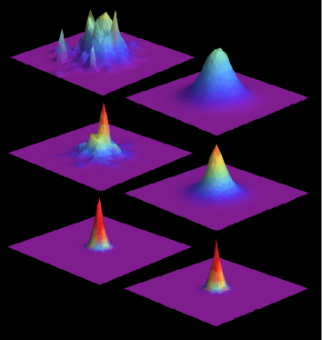
The functioning of our equation is visualized in Fig. 1. We simulate a 3D Bose gas containing 200 particles, trapped in a quartic potential $V(x,y,z)=x^{4}+y^{4}+z^{4}$ and determine the momentum densities $n(p_{x},p_{y})$ (the third momentum $p_{z}$ is integrated over). Three different temperatures are chosen: above (top), at (middle), and below (bottom) the critical temperature for Bose-Einstein condensation. While on the left hand side we display a single realization of eq. (Stochastic field equation for the canonical ensemble of a Bose gas) after a certain propagation time, the right hand side shows time averages over 15000 time steps. Obviously, on average we obtain the typical pictures for the transition to a Bose-Einstein condensate.

The true quality of our equation is to be verified by calculating various characteristic quantities. As shown in Fig. 1, the numerical code in position representation allows us to treat the Bose gas in any trapping potential. In order to make contact to previous results for the canonical ensemble, however, we restrict ourselves in the following to a 3D box and a 3D harmonic oscillator potential. More general considerations will be published elsewhere hellerstrunz02 .

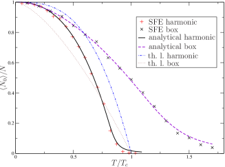
First we show the ground state occupation in Fig. 2. The results for the harmonic oscillator (with $N=200$ particles, plus signs) are obtained by propagating equ. (Stochastic field equation for the canonical ensemble of a Bose gas) on a position grid. No use is made of the known spectrum and eigenfunctions. We compare with an analytical approximation (full line) Koc00 , which is known to be in good agreement with exact results, and the thermodynamic limit (dashed-dotted line). Next we show results for a 3D box ($N=100$ particles, crosses) obtained from our SFE (here computed in momentum space) compared with an (approximate) result based on a path integral approach Gla07 (dashed line) and find very good agreement. Temperature is scaled to the critical temperature of the thermodynamic limit Pet02 ; Pit03 . Note that finite size effects are very significant for the box as seen when comparing with the thermodynamic limit (dotted line).

Figure 3: First and second order spatial correlations $G_{1}(x,0)$ (top) and $G_{2}(x,0)$ (bottom) for a Bose gas in a 3D box potential with periodic boundary conditions (left) and a 3D harmonic oscillator potential (right) for different temperatures. Results from the SFE (plus signs, crosses, stars) are compared to a direct calculation based on the theory of Nar99 : a grand-canonical description (“gc”, solid, dashed and dashed-dotted lines) fails for $G_{2}$, while a corrected theory (“gc+c” dashed-dotted and dotted lines) shows good agreement.

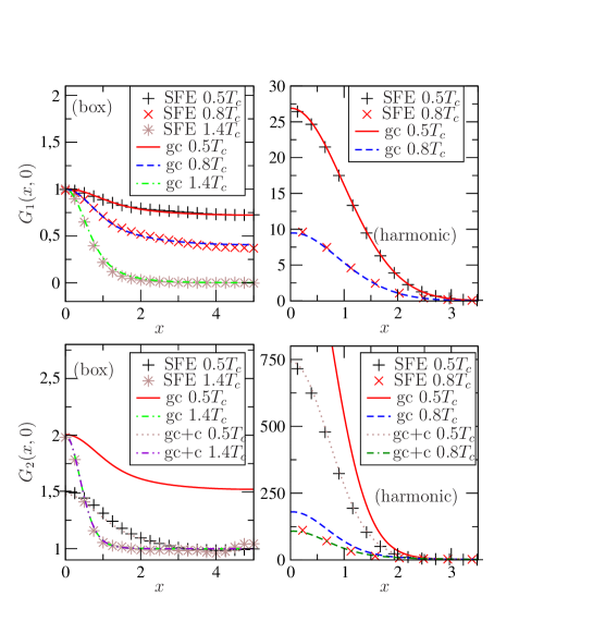
Next we determine spatial correlation functions of first $G_{1}(x,x^{\prime})=\langle\hat{\psi}^{\dagger}(x)\hat{\psi}(x^{\prime})\rangle_{N}$ and second order $G_{2}(x,x^{\prime})=\langle\hat{\psi}^{\dagger}(x)\hat{\psi}^{\dagger}(x^{\prime})\hat{\psi}(x)\hat{\psi}(x^{\prime})\rangle_{N}$ above and below the critical temperature. $G_{1}$ can be measured through interference experiments (see Blo00 ). $G_{2}$ and related quantities have been measured more recently in impressive experiments Hel03 ; Foe05 ; Oet05 ; Sch05 . For first order correlations, the canonical results are close to the grand canonical values. For second order correlations and temperatures below the critical temperature, however, large deviations appear and the results of the canonical ensemble may be obtained approximately with the help of condensate corrections to the grand canonical calculation Nar99 . In Fig. 3, we show $G_{1}(x,0)$ (top) and $G_{2}(x,0)$ (bottom) obtained from the SFE (Stochastic field equation for the canonical ensemble of a Bose gas); here for a 3D Bose gas of $1000$ particles in a box with periodic boundary conditions (left hand side) and for a gas of $200$ particles in an isotropic harmonic oscillator (right hand side). Our values (plus signs, crosses, stars) are compared with a direct grand canonical calculation (“gc” in Fig. 3) and the corrected description (“gc+c” in Fig. 3) based on the theory of Nar99 . These corrected second order correlation functions are in good agreement with our exact canonical calculations.

We see the main achievement of this paper in the fact that we established a numerically very robust (exact) SFE for the canonical state of an ideal Bose gas, amenable to an efficient numerical solution in full 3D for arbitrary trapping potentials. Still, in the light of the wealth of activities involving ultracold quantum gases, it is certainly of great importance to also investigate the interacting case. Let us therefore relate equ. (Stochastic field equation for the canonical ensemble of a Bose gas) to previous stochastic equations constructed for the grand canonical ensemble of an interacting Bose gas Sto97 ; Dav01 ; Gar02 ; Bra05 ; Khe04 . A good survey over these different findings, their relations and their limitations is given in Bra05 . Most notably, in several of these approaches Sto97 ; Dav01 ; Gar02 ; Bra05 , termed “classical field methods” in Bra05 (and see also Hoh77 ), due to ultraviolet problems, lowly occupied states must be cut off Dav01 or treated in a different formalism Gar02 ; Bra05 .

Let us now turn to our SFE (Stochastic field equation for the canonical ensemble of a Bose gas): omitting the non-linear terms and substituting both $H\rightarrow{\tilde{H}}=H-\mu{\hat{N}}$ and $\widehat{kT}\rightarrow\widetilde{kT}={\tilde{H}}/(e^{{\tilde{H}}/kT}-1)$ ($\mu$ the chemical potential and ${\hat{N}}$ the number operator), equ. (Stochastic field equation for the canonical ensemble of a Bose gas) reduces to

$$d|\psi\rangle=-(\Lambda+i)\tilde{H}|\psi\rangle+\sqrt{2\Lambda\widetilde{kT}}\;|d\xi\rangle$$ (5)

of which one can easily show that it indeed provides proper grand canonical ensemble averages hellerstrunz03 . We hasten to stress that the canonical equation (Stochastic field equation for the canonical ensemble of a Bose gas) is not merely a normalized version of equ.(5). As discussed before, in (5) the operator $\widetilde{kT}$ incorporates a natural high energy noise cutoff induced by proper quantum statistics. No further care is required.

Describing a grand canonical ensemble, equ. (5) is the link to establish a connection to the “classical field methods” mentioned above for an interacting gas: First, the operator $\widetilde{kT}$ appears as the simple temperature $kT$ in those approaches, requiring a cutoff. More importantly, the interaction may be taken into account by a mean field contribution ${\tilde{H}}\rightarrow{\tilde{H}}+g|\psi(x)|^{2}$, where $g=4\pi a\hbar^{2}/m$ is the interaction parameter and $a$ the s-wave scattering length.

After these considerations it appears more than tempting to use equation (Stochastic field equation for the canonical ensemble of a Bose gas) for a canonical ensemble even in the case of a weakly interacting gas, with $V(x)\rightarrow V(x)+g|\psi(x)|^{2}$. As argued, the resulting equation is free from ultraviolet problems and coincides (in the grand canonical case) with previous (“classical”) equations (including interaction and a high-energy cutoff). Moreover, it reduces to the (imaginary-time) Gross-Pitaevskii equation for $kT\rightarrow 0$, describing a pure condensate (with the given particle number $N$).

Let us briefly summarize our result: we present a norm-preserving stochastic field equation for the canonical state of a Bose gas, describing experiments with a finite number of atoms in an arbitrary trap. Being driven by spatially correlated noise, cut-off issues do not appear; the equation is numerically very stable. We stress that it is valid for arbitrary temperatures: for $T\gg T_{c}$ it provides a wave description of a classical gas of massive particles. This is very much in the spirit of the way we think of light emerging from a light bulb as being composed of incoherent wave trains. We are able to determine important quantities like spatial correlation functions and occupation numbers as a function of temperature in arbitrary traps. Finally, we relate our equation to stochastic Gross-Pitaevskii equations that exist for interacting gases in the grand canonical ensemble, raising expectations that the new equation should be applicable to weakly interacting Bose gases as well.

We are grateful for inspiring discussions with Markus Oberthaler and Thimo Grotz. S. H. acknowledges support by the International Max Planck Research School for Dynamical Processes in Atoms, Molecules and Solids, Dresden.

References

- (1) C. J. Pethick and H. Smith, Bose-Einstein Condensation In Dilute Gases (Cambridge University Press, Cambridge, 2002).
- (2) L. Pitaevskii and S. Stringari, Bose-Einstein Condensation (Oxford University Press, Oxford, 2003).
- (3) I. Bloch, J. Dalibard, and W. Zwerger, Rev. Mod. Phys. 80, 885 (2008).
- (4) R. M. Ziff, G. E. Uhlenbeck, and M. Kac, Phys. Rep. 32, 169 (1977).
- (5) I. Bloch, T. W. Hänsch, and T. Esslinger, Nature 403, 166 (2000).
- (6) D. Hellweg, L. Cacciapuoti, M. Kottke, T. Schulte, K. Sengstock, W. Ertmer, and J. J. Arlt, Phys. Rev. Lett. 91, 010406 (2003).
- (7) S. Fölling, F. Gerbier, A. Widera, O. Mandel, T. Gericke, and I. Bloch, Nature 434, 481 (2005).
- (8) A. Öttl, S. Ritter, M. Köhl and T. Esslinger, Phys. Rev. Lett. 95, 090404 (2005).
- (9) M. Schellekens, R. Hoppeler, A. Perrin, J. V. Gomes, D. Boiron, A. Aspect and C. I. Westbrook, Science 310, 648 (2005).
- (10) H. T. C. Stoof, Phys. Rev. Lett. 78, 768 (1997); H. T. C. Stoof and M. J. Bijlsma, J. Low. Temp. Phys. 124, 431 (2001); R. A. Duine and H. T. C. Stoof, Phys. Rev. A 65, 13603 (2001).
- (11) M. J. Davis, S. A. Morgan, and K. Burnett, Phys. Rev. Lett. 87, 0160402 (2001); M. J. Davis, R. J. Ballagh, and K. Burnett, J. Phys. B: At. Mol. Opt. Phys. 34, 4487 (2001).
- (12) C. W. Gardiner, J. R. Anglin, and T. I. A. Fudge, J. Phys. B: At. Mol. Opt. Phys. 35, 1555 (2002).
- (13) A. S. Bradley, P. B. Blakies and C. W. Gardiner, J. Phys. B: At. Mol. Opt. Phys. 38, 4259 (2005).
- (14) P. D. Drummond, P. Deuar, and K. V. Kheruntsyan, Phys. Rev. Lett. 92, 040405 (2004); P. Deuar and P. D. Drummond, J. Phys. A 39, 1163 (2006); P. Deuar and P. D. Drummond, J. Phys. A 39, 2723 (2006).
- (15) C. W. Gardiner, Handbook of Stochastic Methods (Springer-Verlag, Berlin Heidelberg, 1983).
- (16) S. Heller and W. T. Strunz (to be published).
- (17) W. P. Schleich, Quantum Optics in Phase Space (Wiley-VCH, Berlin, 2001).
- (18) B. R. Mollow, Phys. Rev. 168, 1896 (1968).
- (19) S. Ritter, A. Öttl, T. Donner, T. Bourdel, M. Köhl, T. Esslinger, Phys. Rev. Lett. 98, 090402 (2007).
- (20) V. V. Kocharovsky, M. O. Scully, S.-Y. Zhu, and M. S. Zubairy, Phys. Rev. A 61, 023609 (2000).
- (21) K. Glaum, H. Kleinert, and A. Pelster, Phys. Rev. A 76, 063604 (2007).
- (22) M. Naraschewski and R. J. Glauber, Phys. Rev. A 59, 4595 (1999).
- (23) P. Hohenberg and B. I. Halperin, Rev. Mod. Phys. 49, 435 (1977).
- (24) S. Heller and W. T. Strunz, to appear in “Path Integrals - new trends and perspectives” by W. Janke and A. Pelster (eds.), (World Scientific, Singapore, 2008).