A phase transition for non-intersecting Brownian motions, and the Painlevé II equation

Abstract

We consider $n$ non-intersecting Brownian motions with two fixed starting positions and two fixed ending positions in the large $n$ limit. We show that in case of ‘large separation’ between the endpoints, the particles are asymptotically distributed in two separate groups, with no interaction between them, as one would intuitively expect. We give a rigorous proof using the Riemann-Hilbert formalism. In the case of ‘critical separation’ between the endpoints we are led to a model Riemann-Hilbert problem associated to the Hastings-McLeod solution of the Painlevé II equation. We show that the Painlevé II equation also appears in the large $n$ asymptotics of the recurrence coefficients of the multiple Hermite polynomials that are associated with the Riemann-Hilbert problem.

Keywords: non-intersecting Brownian motions, Riemann-Hilbert problem, Deift-Zhou steepest descent analysis, Painlevé II equation, multiple Hermite polynomials, recurrence coefficients.

1 Introduction and statement of results

1.1 Non-intersecting Brownian motion

This paper deals with non-intersecting Brownian motions with two fixed starting positions $a_{1}$, $a_{2}$ and two fixed ending positions $b_{1}$, $b_{2}$. Let us first describe the general framework in which this paper fits.

Let $p,q\in\mathbb{N}$. Consider sequences of real numbers $\{a_{k}\}_{k=1}^{p}$, $\{b_{l}\}_{l=1}^{q}$ and sequences of positive integers $\{n_{k}\}_{k=1}^{p}$, $\{m_{l}\}_{l=1}^{q}$ satisfying

• $a_{1}>\cdots>a_{p}$,

• $b_{1}>\cdots>b_{q}$,

• $\sum_{k=1}^{p}n_{k}=\sum_{l=1}^{q}m_{l}=:n$.

Consider $n$ one-dimensional Brownian motions (actually Brownian bridges) such that $n_{k}$ of them start from the point $a_{k}$ at time $t=0$, for $k=1,\ldots,p$, and $m_{l}$ of them arrive in the point $b_{l}$ at time $t=1$, for $l=1,\ldots,q$, and such that the $n$ particles are conditioned not to collide with each other in the time interval $t\in(0,1)$.

We are interested in the limiting behavior where the number of Brownian particles $n$ tends to infinity in such a way that each of the fractions $n_{k}/n$, $k=1,\ldots,p$ and $m_{l}/n$, $l=1,\ldots,q$ has a limit in $(0,1)$. To obtain non-trivial limiting behavior we assume that the transition probability density of the Brownian motions scales as

$$P_{N}(t,x,y)=\frac{\sqrt{N}}{\sqrt{2\pi t}}e^{-\frac{N}{2t}(x-y)^{2}}$$ (1.1)

where $N$ is a parameter (the inverse of the overall variance) that increases as $n$ increases. In a non-critical regime we will simply take $N=n$.

Under these assumptions, it is expected that the particles will asymptotically fill a bounded region in the time-space plane ($tx$-plane). It is also expected that for every $t\in(0,1)$, the particles at time $t$ are asymptotically distributed according to some well-defined limiting distribution. See Figures 1 and 2 for possible behaviors when $p=q=1$ and $p=q=2$, respectively.

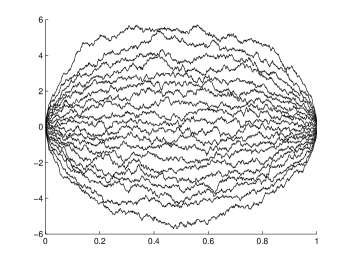
Figure 1: Non-intersecting Brownian motions in case of one starting and ending point. Here the horizontal axis denotes the time, $t\in[0,1]$, and for each fixed $t$ the positions of the $n$ non-intersecting Brownian motions at time $t$ are denoted on the vertical line through $t$.

It is natural to ask for an explicit description of this limiting distribution. Such a result is known in the classical case where $p=q=1$, which is connected to Dyson’s Brownian motion [19]. Here it is known that up to a suitable scaling and translation, the Brownian particles at time $t\in(0,1)$ have the same joint distribution as the eigenvalues of the Gaussian unitary ensemble (GUE) of size $n\times n$, and the limiting distribution as $n\to\infty$ is given by Wigner’s semicircle law. More precisely, if all Brownian motions start from $a:=a_{1}$ at time $t=0$ and end up at $b:=b_{1}$ at time $t=1$, and if $N=n/T$, then the non-intersecting Brownian particles at time $t\in(0,1)$ are asymptotically distributed on the interval $[\alpha(t),\beta(t)]$ with endpoints

$$\alpha(t) =(1-t)a+tb-\sqrt{4Tt(1-t)},$$ (1.2)

$$\beta(t) =(1-t)a+tb+\sqrt{4Tt(1-t)},$$ (1.3)

and with limiting density of the particles given by the semicircle law on that interval

$$\frac{1}{2\pi Tt(1-t)}\sqrt{(\beta(t)-x)(x-\alpha(t))},\qquad x\in[\alpha(t),\beta(t)].$$ (1.4)

By varying $t\in[0,1]$, the endpoints (1.2), (1.3) parameterize an ellipse in the time-space plane, see Figure 1.

Explicit descriptions of the limiting distribution of the non-intersecting Brownian motions are also known when $p=1$, $q>1$. Also in this case there is an underlying random matrix model [3, 7, 8, 27, 31, 32].

The limiting distribution is also known when $p=q=2$, $m_{1}=n_{1}=m_{2}=n_{2}=n/2$, $N=n$, and $(a_{1}-a_{2})(b_{1}-b_{2})<2$. In this case the limiting distribution as $n\to\infty$ of the Brownian particles at time $t\in(0,1)$ is obtained from a certain algebraic curve of degree four [15]. In contrast to the previous cases, however, it is not known if the Brownian particles for finite $n$ can be described as the eigenvalues of a random matrix ensemble. See Figure 2 for an illustration of this case.

1.2 Separation of the endpoints

The main results of this paper will concern non-intersecting Brownian motions with two starting points $a_{1}>a_{2}$ at time $t=0$, two ending points $b_{1}>b_{2}$ at time $t=1$, and in addition

$$n_{1}=m_{1},\qquad n_{2}=m_{2},\quad(\textrm{for all }n)$$ (1.5)

and if we put

$$p_{1}=\frac{n_{1}}{n},\qquad p_{2}=\frac{n_{2}}{n}$$ (1.6)

which are varying with $n$, then we assume that

$$\frac{n_{1}}{n} =p_{1}=p_{1}^{*}+O(1/n),\quad n\to\infty,$$ (1.7)

$$\frac{n_{2}}{n} =p_{2}=p_{2}^{*}+O(1/n),\quad n\to\infty,$$ (1.8)

for certain limiting values $p_{1}^{*},p_{2}^{*}\in(0,1)$. We also assume that $N$ increases with $n$ such that

$$T=n/N>0$$ (1.9)

is fixed.

If the assumptions (1.5)–(1.9) hold, and if the separation between the starting points $a_{1}$ and $a_{2}$, and the ending points $b_{1}$ and $b_{2}$ is large enough, then in analogy with (1.2)–(1.4), one would expect the Brownian particles to be asymptotically distributed on two disjoint ellipses in the $tx$-plane, whose intersections with the vertical line through $t$ are given by the two intervals $[\alpha_{1}^{*},\beta_{1}^{*}]$ and $[\alpha_{2}^{*},\beta_{2}^{*}]$ with

$$\alpha_{j}^{*} =\alpha_{j}^{*}(t)=(1-t)a_{j}+tb_{j}-\sqrt{4p_{j}^{*}Tt(1-t)},$$ (1.10)

$$\beta_{j}^{*} =\beta_{j}^{*}(t)=(1-t)a_{j}+tb_{j}+\sqrt{4p_{j}^{*}Tt(1-t)},$$ (1.11)

for $j=1,2$, and with limiting densities on these two intervals given by the semicircle laws

$$\frac{1}{2\pi Tt(1-t)}\sqrt{(\beta_{j}^{*}-x)(x-\alpha_{j}^{*})},\quad x\in[\alpha_{j}^{*},\beta_{j}^{*}],\quad j=1,2,$$ (1.12)

for each $t\in(0,1)$. This situation is illustrated in Figure 2. Note that

$$\frac{1}{2\pi Tt(1-t)}\int_{\alpha_{j}^{*}}^{\beta_{j}^{*}}\sqrt{(\beta_{j}^{*}-x)(x-\alpha_{j}^{*})}dx=p_{j}^{*}.$$

We derive the precise condition for this two-ellipse scenario to happen. It is clear that a necessary condition is the disjointness of the two ellipses.

Lemma 1.1.

(Disjointness of the two ellipses) The two ellipses parameterized by (1.10)–(1.11) are disjoint if and only if

$$(a_{1}-a_{2})(b_{1}-b_{2})>T\left(\sqrt{p_{1}^{*}}+\sqrt{p_{2}^{*}}\right)^{2}.$$ (1.13)

proof. The two ellipses are disjoint if and only if $\alpha_{1}^{*}(t)>\beta_{2}^{*}(t)$ for all $t\in(0,1)$. From (1.10)–(1.11) this leads to the condition

$$(1-t)(a_{1}-a_{2})+t(b_{1}-b_{2})>\sqrt{4Tt(1-t)}\left(\sqrt{p_{1}^{*}}+\sqrt{p_{2}^{*}}\right),\quad t\in(0,1),$$ (1.14)

which after putting $u=\sqrt{\frac{t}{1-t}}$ is equivalent to

$$u^{2}(b_{1}-b_{2})-2u\sqrt{T}\left(\sqrt{p_{1}^{*}}+\sqrt{p_{2}^{*}}\right)+(a_{1}-a_{2})>0,\qquad u\in(0,\infty).$$

The left-hand side is a quadratic expression in $u$, whose discriminant is negative if and only if (1.13) holds. The lemma then easily follows since $b_{1}>b_{2}$ and $a_{1}>a_{2}$. $\hfill\square\\$

We will call (1.13) the case of large separation.

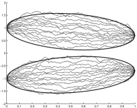
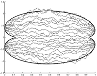
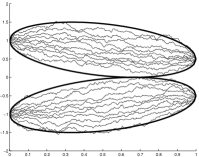
Figure 2: Non-intersecting Brownian motions with two starting and two ending positions in case of (a) large, (b) small, and (c) critical separation between the endpoints. Here the horizontal axis denotes the time, $t\in[0,1]$, and for each fixed $t$ the positions of the $n$ non-intersecting Brownian motions at time $t$ are denoted on the vertical line through $t$. Note that for $n\to\infty$ the positions of the Brownian motions fill a prescribed region in the time-space plane, which is bounded by the boldface lines in the figures. Here we have chosen $N=n=20$ and $p_{1}=p_{2}=1/2$ in each of the figures, and (a) $a_{1}=-a_{2}=1$, $b_{1}=-b_{2}=0.7$, (b) $a_{1}=-a_{2}=0.4$, $b_{1}=-b_{2}=0.3$, and (c) $a_{1}=-a_{2}=1$, $b_{1}=-b_{2}=1/2$, in the cases of large, small and critical separation, respectively.

Definition 1.2.

(Large, critical and small separation) For each $n$, consider $n$ non-intersecting Brownian motions with two starting points $a_{1}>a_{2}$ at time $t=0$ and two ending points $b_{1}>b_{2}$ at time $t=1$, and assume that the hypotheses (1.5)–(1.9) hold. If (1.13) holds, we say that we are in a situation of large separation of the endpoints. If instead

$$(a_{1}-a_{2})(b_{1}-b_{2})<T(\sqrt{p_{1}^{*}}+\sqrt{p_{2}^{*}})^{2},$$ (1.15)

we are in a situation of small separation, and if

$$(a_{1}-a_{2})(b_{1}-b_{2})=T(\sqrt{p_{1}^{*}}+\sqrt{p_{2}^{*}})^{2},$$ (1.16)

we are in a situation of critical separation between the endpoints. In the latter case, we define the critical time $t_{\textrm{crit}}\in(0,1)$ as

$$t_{\textrm{crit}}=\frac{a_{1}-a_{2}}{(a_{1}-a_{2})+(b_{1}-b_{2})}.$$ (1.17)

The non-intersecting Brownian motions corresponding to each of these three cases are illustrated in Figure 2–2. In the case of critical separation, the time $t_{\textrm{crit}}$ is precisely the time where the two ellipses with endpoints parameterized by (1.10)–(1.11) are tangent, cf. Figure 2.

We may equivalently view the critical behavior in terms of the temperature parameter $T=n/N$. With $a_{j}$, $b_{j}$, and $p_{j}^{*}$ fixed for $j=1,2$, there is a critical temperature

$$T_{\textrm{crit}}=\frac{(a_{1}-a_{2})(b_{1}-b_{2})}{(\sqrt{p_{1}^{*}}+\sqrt{p_{2}^{*}})^{2}}$$

such that $T<T_{\textrm{crit}}$ (low temperature), $T>T_{\textrm{crit}}$ (high temperature), and $T=T_{\textrm{crit}}$ (critical temperature) correspond to large, small, and critical separation, respectively.

1.3 Large separation: decoupling of the Brownian motions

The case of small separation of the endpoints was considered in [15] for the special case when $p_{1}=p_{2}=1/2$. In the present paper, we will focus instead on the cases of large and critical separation. As is to be expected, in these regimes the Brownian motions asymptotically decouple into two separate groups, as is evidenced by Figures 2 and 2. This is our first main theorem.

Theorem 1.3.

(Decoupling of Brownian motions) Consider $n$ non-intersecting Brownian motions with two starting points $a_{1}>a_{2}$ at time $t=0$ and two ending points $b_{1}>b_{2}$ at time $t=1$. Assume that the hypotheses (1.5)–(1.9) hold, and assume that either

• there is large separation of the endpoints (1.13), or

• there is critical separation of the endpoints (1.16) and $t\neq t_{\textrm{crit}}$, where $t_{\textrm{crit}}$ is given by (1.17).

Then as $n\to\infty$ the Brownian particles at time $t\in(0,1)$ are asymptotically supported on the two disjoint intervals $[\alpha_{1}^{*}(t),\beta_{1}^{*}(t)]$ and $[\alpha_{2}^{*}(t),\beta_{2}^{*}(t)]$ given by (1.10)–(1.11), with limiting densities given by the semicircle laws (1.12).

In the case of critical separation, we strongly expect that the conclusion of the theorem should also be valid when $t=t_{\textrm{crit}}$. However, we will not consider the critical time in this paper.

Our proof of Theorem 1.3 follows from a steepest descent analysis of the underlying Riemann-Hilbert problem that will be described in Section 1.4. The Riemann-Hilbert problem is of size $4\times 4$ and it was also used in [15] to analyze the case of small separation. In the (apparently) simpler case of large separation one expects that for large $n$, the $4\times 4$ RH problem asymptotically decouples into two smaller RH problems of size $2\times 2$. This is indeed the case, but in order to show this, we need a preliminary transformation where we introduce auxiliary curves in the complex plane and subsequently perform a Gaussian elimination step in the jump matrix of the RH problem, serving to annihilate some undesired entries of this matrix. This Gaussian elimination step is similar to the so-called global opening of the lens discussed in [3, 4, 15, 29].

It follows from our analysis that the interaction between the two groups of Brownian particles decays exponentially with $n$ in case of large separation, and polynomially (like a power $n^{-1/3}$) in case of critical separation at a non-critical time. In the limit when $n\to\infty$ the particles will then indeed be distributed inside two disjoint ellipses in the time-space plane.

1.4 Riemann-Hilbert problem

The non-intersecting Brownian motions described in the previous subsections are related to the following Riemann-Hilbert problem (RH problem) which we already alluded to above. The RH problem was introduced in [14] as a generalization of the RH problem for orthogonal polynomials in [22], see also [37]. In accordance with Section 1.1 we will state the RH problem for general numbers of starting and ending positions $p,q$ of the Brownian motions, although in our applications we will eventually take $p=q=2$.

Define weight functions

$$w_{1,k}(x) =e^{-\frac{N}{2t}(x^{2}-2a_{k}x)},\quad k=1,\ldots,p,$$ (1.18)

$$w_{2,l}(x) =e^{-\frac{N}{2(1-t)}(x^{2}-2b_{l}x)},\quad l=1,\ldots,q.$$ (1.19)

The RH problem consists in finding a matrix-valued function $Y(z)=$
$Y_{n_{1},\ldots,n_{p};m_{1},\ldots,m_{q}}(z)$ of size $p+q$ by $p+q$ such that

• $Y(z)$ is analytic in $\mathbb{C}\setminus\mathbb{R}$;

• For $x\in\mathbb{R}$, it holds that

  $$Y_{+}(x)=Y_{-}(x)\begin{pmatrix}I_{p}&W(x)\\ 0&I_{q}\end{pmatrix},$$ (1.20)

  where $I_{k}$ denotes the identity matrix of size $k$; where $W(x)$ denotes the rank-one matrix (outer product of two vectors)

  $$W(x)=\begin{pmatrix}w_{1,1}(x)\\ \vdots\\ w_{1,p}(x)\end{pmatrix}\begin{pmatrix}w_{2,1}(x)&\ldots&w_{2,q}(x)\end{pmatrix},$$ (1.21)

  and where the notation $Y_{+}(x),Y_{-}(x)$ denotes the limit of $Y(z)$ with $z$ approaching $x\in\mathbb{R}$ from the upper or lower half plane in $\mathbb{C}$, respectively;

• As $z\to\infty$, we have that

  $$Y(z)=(I_{p+q}+O(1/z))\operatorname{diag}(z^{n_{1}},\ldots,z^{n_{p}},z^{-m_{1}},\ldots,z^{-m_{q}}).$$ (1.22)

The RH problem has a unique solution [14] that can be described in terms of certain multiple orthogonal polynomials (actually multiple Hermite polynomials); details will be given in Section 1.6.

Let us explain the connection between the non-intersecting Brownian motions and the RH problem in the case $p=q=2$. It is well-known [25], see also [24, 26], that the distribution of the non-intersecting Brownian motions at time $t\in(0,1)$ describes a determinantal point process, determined by an associated correlation kernel. According to [14] the correlation kernel $K(x,y)=K_{n_{1},n_{2};m_{1},m_{2}}(x,y)$ can be expressed in terms of the solution to the RH problem as

$$K(x,y)=\frac{1}{2\pi i(x-y)}\begin{pmatrix}0&0&w_{2,1}(y)&w_{2,2}(y)\end{pmatrix}Y_{+}^{-1}(y)Y_{+}(x)\begin{pmatrix}w_{1,1}(x)\\ w_{1,2}(x)\\ 0\\ 0\end{pmatrix}.$$ (1.23)

By general properties of determinantal point processes, Theorem 1.3 then comes down to the statement that under the conditions of Theorem 1.3, the limit of $\frac{1}{n}K_{n_{1},n_{2};n_{1},n_{2}}(x,x)$ as $n\to\infty$ exists and is equal to

$$\lim_{n\to\infty}\frac{1}{n}K_{n_{1},n_{2};n_{1},n_{2}}(x,x)=\frac{1}{2\pi Tt(1-t)}\sqrt{(\beta_{j}^{*}-x)(x-\alpha_{j}^{*})},\qquad x\in[\alpha_{j}^{*},\beta_{j}^{*}],$$ (1.24)

for $j=1,2$. This is what we will show in Sections 2 and 3.

Our method will also allow us to obtain the local scaling limits of the correlation kernel that are common in random matrix theory and related areas, namely the sine kernel in the bulk and the Airy kernel at the endpoints of the intervals $[\alpha_{1}^{*},\beta_{1}^{*}]$ and $[\alpha_{2}^{*},\beta_{2}^{*}]$. We will not go into details about this in this paper.

1.5 Critical separation and the double scaling limit

Assume that the endpoints are such that

$$(a_{1}-a_{2})(b_{1}-b_{2})=(\sqrt{p_{1}^{*}}+\sqrt{p_{2}^{*}})^{2}.$$ (1.25)

We put

$$N=n/T$$

where $T$ can be interpreted as a temperature variable. For $T=1$ (critical temperature) we have by (1.16), (1.25) and Theorem 1.3 that in the large $n$ limit, the particles fill out two ellipses, which are tangent to each other at the critical time $t_{\textrm{crit}}$, see Figure 2. By varying $T$ around the critical value $T_{\textrm{crit}}=1$ we move from a case of disjoint ellipses (for $T<1$) to a case of small separation (for $T>1$), where the two-ellipses scenario is not valid anymore. Hence we see a phase transition in the case of critical separation, which is clearly seen at the critical time $t_{\textrm{crit}}$. At a non-critical time $t\neq t_{\textrm{crit}}$ the phase transition is less obvious, but there is also a nontrivial transitional effect. Indeed, the distribution of particles at time $t\neq t_{\textrm{crit}}$ in the case of small separation differs from the distribution of two semicircle laws of two disjoint intervals, which it is for large separation. Hence the endpoints of the intervals do not depend analytically on the starting and ending points, which indicates the phase transition. It is a surprising outcome of our analysis that the phase transition for the case where $t\neq t_{\textrm{crit}}$ can be described by the Painlevé II equation.

In the case of critical separation we investigate the behavior of the Brownian particles in a double scaling limit where $n,N\to\infty$, and simultaneously $T\to T_{\textrm{crit}}=1$. More precisely, we consider the endpoints $a_{1}$, $a_{2}$, $b_{1}$, $b_{2}$ fixed so that (1.25) holds for all $n$. The temperature $T=T_{n}=n/N$ is varying with $n$ as follows:

$$T_{n}=1+Ln^{-2/3},$$ (1.26)

where $L$ is an arbitrary real constant.

We will show that in the double scaling regime described above, the steepest descent analysis of the Riemann-Hilbert problem leads in a natural way to a model Riemann-Hilbert problem related to the Painlevé II equation. More precisely, we will be led to the construction of a local parametrix that can be mapped onto the model RH problem [20] satisfied by the $\Psi$-functions (Lax pair) associated with the Hastings-McLeod solution of the Painlevé II equation

$$q^{\prime\prime}(s)=sq(s)+2q^{3}(s).$$ (1.27)

The Hasting-McLeod solution [23] is the special solution $q(s)$ of (1.27) which is real for real $s$ and satisfies $q(s)\sim\textrm{Ai}(s)$ as $s\to\infty$, where Ai denotes the usual Airy function. The precise form of the model RH problem will be described in Section 3.3.

The Hastings-McLeod solution of the Painlevé II equation also appears in the famous Tracy-Widom distributions [34, 35] for the largest eigenvalues of large random matrices. It also appears in the critical unitarily invariant matrix models, where the parameters in the model are fine-tuned so that the limiting mean eigenvalue density vanishes quadratically at an interior point of its support [6, 11]. In this case it leads to a new family of local scaling limits of the eigenvalue correlation kernel that involve the $\Psi$-functions associated with $q(s)$.

In our situation the Painlevé II equation does not manifest itself in the local scaling limits of the correlation kernel. The construction of the local parametrix is done at a point $x_{0}$ strictly outside of the support and it does not influence the local correlation functions for the positions of any of the particles. The point $x_{0}$ does not seem to have any physical meaning.

We emphasize that our asymptotic analysis will be only valid when $t\neq t_{\textrm{crit}}$. At the critical time $t=t_{\textrm{crit}}$ where the two ellipses are tangent, one is led to a considerably more difficult, multi-critical situation. Here one expects the appearance of a model RH problem related to some as yet unknown fourth order ODE. As already mentioned, we will not attempt to study this case in the present paper.

1.6 Generalities on multiple orthogonal polynomials

While the appearance of the Hastings-McLeod solution of the RH problem does not affect any of the local scaling limits, it is felt by the recurrence coefficients of the multiple Hermite polynomials. These polynomials appear in the solution of the RH problem given in Section 1.4.

To state the results, let us first recall some generalities on multiple orthogonal polynomials in the sense of [14]. In accordance with Sections 1.1 and 1.4 we will again give the definitions for general values of $p$ and $q$, although in our applications we will eventually take $p=q=2$.

Definition 1.4.

(Multiple orthogonal polynomials; cf. [14]) Let $p,q\in\mathbb{N}$ be two positive integers. Let there be given

• A (finite) sequence of positive integers $n_{1},n_{2},\ldots,n_{p}\in\mathbb{N}$;

• A sequence of weight functions $w_{1,1}(x),w_{1,2}(x),\ldots,w_{1,p}(x):\mathbb{R}\to\mathbb{R}$;

• A sequence of positive integers $m_{1},m_{2},\ldots,m_{q}\in\mathbb{N}$;

• A sequence of weight functions $w_{2,1}(x),w_{2,2}(x),\ldots,w_{2,q}(x):\mathbb{R}\to\mathbb{R}$.

Put $\mathbf{n}:=(n_{1},\ldots,n_{p})$, $|\mathbf{n}|:=\sum_{k=1}^{p}n_{k}$ and similarly for $\mathbf{m}$ and $|\mathbf{m}|$. Assume $|\mathbf{n}|=|\mathbf{m}|+1$. We say that a sequence of polynomials $A_{1}(x),A_{2}(x),\ldots,A_{p}(x)$ is multiple orthogonal with respect to the above data if (i) the polynomials $A_{k}(x)$ have degrees bounded by $n_{k}-1$:

$$\deg A_{k}\leq n_{k}-1,\quad k=1,\ldots,p,$$ (1.28)

and (ii) the function

$$Q(x):=\sum_{k=1}^{p}A_{k}(x)w_{1,k}(x)$$ (1.29)

satisfies the orthogonality relations

$$\int_{-\infty}^{\infty}Q(x)x^{j}w_{2,l}(x)\ dx=0,$$ (1.30)

for $j=0,1,\ldots,m_{l}-1$ and $l=1,\ldots,q$.

Note that (1.30) states that $Q(x)$ has $m_{l}$ vanishing moments with respect to the weight $w_{2,l}(x)$, $l=1,\ldots,q$.

A schematic illustration of Definition 1.4 is shown in Figure 3. Let us comment on this figure. The left part of the figure shows the polynomials $A_{k}(x)$ and their corresponding number of free coefficients $n_{k}$, $k=1,\ldots,p$. The middle part of the figure shows how the polynomials $A_{k}(x)$ should be assembled into the function $Q(x)$ defined in (1.29). Finally, the right part of the figure schematically shows the orthogonality relations of $Q(x)$ with respect to the different weights $w_{2,l}(x)$, and it shows next to each weight $w_{2,l}(x)$ also the number of vanishing moments $m_{l}$ of $Q(x)$ with respect to this weight.

Figure 3: The figure shows a schematic illustration of the multiple orthogonal polynomials $A_{k}(x)$ in Definition 1.4.

We will refer to the polynomials $A_{k}(x)$ in Definition 1.4 as multiple orthogonal polynomials (MOP). Note that these polynomials were called multiple orthogonal polynomials of mixed type in [14] and mixed MOPs in [2]. We will also find it convenient to use the vectorial notation $\mathbf{A}(x)=(A_{1}(x),\ldots,A_{p}(x))$. To stress the dependence on the multi-indices $\mathbf{n}$, $\mathbf{m}$ we will sometimes write $\mathbf{A}(x)=\mathbf{A}_{\mathbf{n},\mathbf{m}}(x)$ and similarly $A_{j}(x)=(A_{j})_{\mathbf{n},\mathbf{m}}(x)$.

The coefficients of the multiple orthogonal polynomials in Definition 1.4 can be found from a homogeneous linear system with $|\mathbf{n}|$ unknowns (polynomial coefficients) and $|\mathbf{m}|$ equations (orthogonality conditions). The restriction $|\mathbf{n}|=|\mathbf{m}|+1$ in Definition 1.4 guarantees that this system has a nontrivial solution. In fact, the solution space to this linear system will be at least one-dimensional. This corresponds to the fact that the MOP are only determined up to some multiplicative factor. If the MOP are unique up to a multiplicative factor then the pair of indices $\mathbf{n},\mathbf{m}$ is called normal [14].

The fact that the multiple orthogonal polynomials are only determined up to some multiplicative factor allows for different choices of normalization.

Definition 1.5.

(Normalization types of MOP; cf.  [14]) Assume the data in Definition 1.4 and assume that $\mathbf{n},\mathbf{m}$ is a normal pair of indices. Then the MOP in Definition 1.4 are said to satisfy

• the normalization of type I with respect to the $l$th index, $l\in\{1,\ldots,q\}$, if the $m_{l}$th moment of $Q(x)$ with respect to $w_{2,l}(x)$ is equal to one, i.e., if

  $$\int_{-\infty}^{\infty}Q(x)x^{m_{l}}w_{2,l}(x)\ dx=1.$$ (1.31)

• the normalization of type II with respect to the $k$th index, $k\in\{1,\ldots,p\}$, if the leading coefficient of $A_{k}(x)$ is equal to one, i.e., if

  $$A_{k}(x)=x^{n_{k}-1}+O(x^{n_{k}-2}).$$ (1.32)

The vectors of MOP $\mathbf{A}_{\mathbf{n},\mathbf{m}}(x)$ corresponding to the above normalizations will be denoted as $\mathbf{A}_{\mathbf{n},\mathbf{m}}^{(I,l)}(x)$ and $\mathbf{A}_{\mathbf{n},\mathbf{m}}^{(II,k)}(x)$, respectively.

The above normalizations might not always be possible. The type $(I,l)$ normalization is not possible in those cases where the integral on the left side of (1.31) is equal to zero. Similarly, the type $(II,k)$ normalization is not possible in those cases where the $k$th polynomial $A_{k}(x)$ has degree strictly smaller than $n_{k}-1$.

As mentioned above, the MOP appear in the solution of the RH problem in Section 1.4. Let us describe this is somewhat more detail.

Recall that in Definition 1.4 we needed the condition $|\mathbf{n}|=|\mathbf{m}|+1$ to ensure the existence of the multiple orthogonal polynomials. But let us now assume that $|\mathbf{n}|=|\mathbf{m}|$. In this case, the definition of MOP makes no sense. Indeed, the coefficients of the MOP would then solve a homogeneous linear system with as many equations as unknowns, which has in general only the trivial solution.

Therefore, to apply the definition of MOP in a meaningful way for a pair of multi-indices satisfying $|\mathbf{n}|=|\mathbf{m}|$, we should first adapt the multi-indices. There are essentially $p+q$ ways to proceed:

1. One can increase one of the components $n_{k}$, i.e., one can work with the pair of multi-indices $\mathbf{n}+\mathbf{e}_{k},\mathbf{m}$, for some $k\in\{1,2,\ldots,p\}$.

2. One can decrease one of the components $m_{l}$, i.e., one can work with the pair of multi-indices $\mathbf{n},\mathbf{m}-\mathbf{e}_{l}$, for some $l\in\{1,2,\ldots,q\}$.

Here $\mathbf{e}_{k}$ denotes the vector which has all its entries equal to zero, except for the $k$th entry which equals one. The length of $\mathbf{e}_{k}$ should be clear from the context.

Let us discuss the MOP corresponding to each of the $p+q$ pairs of multi-indices above. In the case of a pair of multi-indices $\mathbf{n}+\mathbf{e}_{k},\mathbf{m}$, we are dealing with multiple orthogonal polynomials where the $k$th polynomial $A_{k}$, $k\in\{1,2,\ldots,p\}$ has increased degree; it will be natural to normalize the resulting MOP such that this $k$th polynomial $A_{k}$ is monic, i.e., to work with a normalization of type $(II,k)$. This leads to the vector of MOP

$$\mathbf{A}^{(II,k)}_{\mathbf{n}+\mathbf{e}_{k},\mathbf{m}}(x)=((A_{1})^{(II,k)}_{\mathbf{n}+\mathbf{e}_{k},\mathbf{m}}(x),\ldots,(A_{p})^{(II,k)}_{\mathbf{n}+\mathbf{e}_{k},\mathbf{m}}(x)).$$ (1.33)

In the case of a pair of multi-indices $\mathbf{n},\mathbf{m}-\mathbf{e}_{l}$, we are dealing with multiple orthogonal polynomials where the $l$th orthogonality condition, $l\in\{1,2,\ldots,q\}$ has a decreased number of vanishing moments; it will be natural to normalize the resulting MOP such that this omitted moment equals one, i.e., to work with a normalization of type $(I,l)$. This leads to the vector of MOP

$$\mathbf{A}^{(I,l)}_{\mathbf{n},\mathbf{m}-\mathbf{e}_{l}}(x)=((A_{1})^{(I,l)}_{\mathbf{n},\mathbf{m}-\mathbf{e}_{l}}(x),\ldots,(A_{p})^{(I,l)}_{\mathbf{n},\mathbf{m}-\mathbf{e}_{l}}(x)).$$ (1.34)

Of course we are assuming here that all type I and type II normalizations in (1.33) and (1.34) exist. It turns out that the existence of each of these $p+q$ vectors of MOP is equivalent to a single condition [15], to which we will loosely refer here as the solvability condition. This condition will always be satisfied in the case of Gaussian weight functions (1.18)–(1.19).

Now we can use the above MOP to solve the RH problem in Section 1.4. Indeed, the $p+q$ vectors of MOP in (1.33), (1.34) are row vectors of length $p$, and they can therefore be stacked into the first $p$ columns of a matrix of size $(p+q)\times(p+q)$. Denote with $\widetilde{Y}(z)$ such a matrix. The entries in the remaining $q$ columns of $\widetilde{Y}(z)$ are defined as Cauchy transforms of the functions $Q^{(II,k)}$ and $Q^{(I,l)}$ defined as in (1.29). More precisely, the last $q$ entries in the rows $k=1,\ldots,p$ of $\widetilde{Y}(z)$ are defined by

$$\frac{1}{2\pi i}\int_{-\infty}^{\infty}\frac{Q^{(II,k)}(x)w_{2,l}(x)}{x-z}\ dx,\qquad l=1,\ldots,q,$$ (1.35)

and in the rows $p+k,\ldots,p+q$ by

$$\frac{1}{2\pi i}\int_{-\infty}^{\infty}\frac{Q^{(I,k)}(x)w_{2,l}(x)}{x-z}\ dx,\qquad l=1,\ldots,q.$$ (1.36)

The fact of the matter is the following.

Theorem 1.6.

(Solution to the Riemann-Hilbert problem; cf. [14]) Let $\mathbf{n},\mathbf{m}$ with $|\mathbf{n}|=|\mathbf{m}|$ be such that the solvability condition holds. Then there exists a unique solution $Y(z)=Y_{\mathbf{n},\mathbf{m}}(z)$ of the RH problem in Section 1.4. This solution is given by

$$Y(z)=D\widetilde{Y}(z),$$

where $\widetilde{Y}(z)$ is the matrix constructed from the MOP as described above, and where $D=\operatorname{diag}(I_{p},-2\pi iI_{q})$.

For example, in the special case where $p=q=2$, the solution $Y(z)$ of the Riemann-Hilbert problem in Section 1.4 is given by the $4\times 4$ matrix

$$Y(z)=D\times\left(\begin{array}[]{cccc}(A_{1})_{\mathbf{n}+\mathbf{e}_{1},\mathbf{m}}^{(II,1)}&(A_{2})_{\mathbf{n}+\mathbf{e}_{1},\mathbf{m}}^{(II,1)}&*&*\\ (A_{1})_{\mathbf{n}+\mathbf{e}_{2},\mathbf{m}}^{(II,2)}&(A_{2})_{\mathbf{n}+\mathbf{e}_{2},\mathbf{m}}^{(II,2)}&*&*\\ (A_{1})_{\mathbf{n},\mathbf{m}-\mathbf{e}_{1}}^{(I,1)}&(A_{2})_{\mathbf{n},\mathbf{m}-\mathbf{e}_{1}}^{(I,1)}&*&*\\ (A_{1})_{\mathbf{n},\mathbf{m}-\mathbf{e}_{2}}^{(I,2)}&(A_{2})_{\mathbf{n},\mathbf{m}-\mathbf{e}_{2}}^{(I,2)}&*&*\\ \end{array}\right),$$ (1.37)

where $D:=\operatorname{diag}(1,1,-2\pi i,-2\pi i)$, and where the entries denoted with $*$ are certain Cauchy transforms as in (1.35) and (1.36). The latter entries will be irrelevant in what follows.

1.7 Recurrence relations for multiple Hermite polynomials

In analogy with the three-term recurrence relations for classical orthogonal polynomials on the real line, one can show that the multiple orthogonal polynomials in Section 1.6 satisfy certain $p+q+1$ term recurrence relations. We will state these relations in the case of multiple Hermite polynomials, i.e., when the weight functions of the MOP are given by the Gaussians (1.18)–(1.19). For simplicity, we assume throughout that $p=q=2$, as in (1.37).

Define the next term in the asymptotic expansion of $Y(z)$ in (1.22) as

$$Y(z)=\left(I+\frac{Y_{1}}{z}+O\left(\frac{1}{z^{2}}\right)\right)\operatorname{diag}(z^{n_{1}},z^{n_{2}},z^{-m_{1}},z^{-m_{2}}).$$ (1.38)

The entries of the matrix $Y_{1}=(Y_{1})_{\mathbf{n},\mathbf{m}}$ in (1.38) will be denoted by $(c_{i,j})_{i,j=1}^{4}$.

Proposition 1.7.

(Recurrence relations for multiple Hermite polynomials) Assume $p=q=2$ and let the weight functions be defined by (1.18)–(1.19). Then the multiple Hermite polynomials in (1.37) satisfy the $5$-term recurrence relations

$$(A_{1})^{(II,1)}_{\mathbf{n}+\mathbf{e}_{1}+\mathbf{e}_{1},\mathbf{m}+\mathbf{e}_{1}}=\left(z-(1-t)a_{1}-tb_{1}+\frac{c_{1,2}c_{2,3}}{c_{1,3}}\right)(A_{1})^{(II,1)}_{\mathbf{n}+\mathbf{e}_{1},\mathbf{m}}\\ -c_{1,2}c_{2,1}(A_{1})^{(II,1)}_{\mathbf{n}+\mathbf{e}_{2},\mathbf{m}}-c_{1,3}c_{3,1}(A_{1})^{(II,1)}_{\mathbf{n},\mathbf{m}-\mathbf{e}_{1}}-c_{1,4}c_{4,1}(A_{1})^{(II,1)}_{\mathbf{n},\mathbf{m}-\mathbf{e}_{2}},$$ (1.39)

$$(A_{1})^{(II,1)}_{\mathbf{n}+\mathbf{e}_{1}+\mathbf{e}_{1},\mathbf{m}+\mathbf{e}_{2}}=\left(z-(1-t)a_{1}-tb_{2}+\frac{c_{1,2}c_{2,4}}{c_{1,4}}\right)(A_{1})^{(II,1)}_{\mathbf{n}+\mathbf{e}_{1},\mathbf{m}}\\ -c_{1,2}c_{2,1}(A_{1})^{(II,1)}_{\mathbf{n}+\mathbf{e}_{2},\mathbf{m}}-c_{1,3}c_{3,1}(A_{1})^{(II,1)}_{\mathbf{n},\mathbf{m}-\mathbf{e}_{1}}-c_{1,4}c_{4,1}(A_{1})^{(II,1)}_{\mathbf{n},\mathbf{m}-\mathbf{e}_{2}},$$ (1.40)

$$(A_{2})^{(II,2)}_{\mathbf{n}+\mathbf{e}_{2}+\mathbf{e}_{2},\mathbf{m}+\mathbf{e}_{1}}=\left(z-(1-t)a_{2}-tb_{1}+\frac{c_{2,1}c_{1,3}}{c_{2,3}}\right)(A_{2})^{(II,2)}_{\mathbf{n}+\mathbf{e}_{2},\mathbf{m}}\\ -c_{2,1}c_{1,2}(A_{2})^{(II,2)}_{\mathbf{n}+\mathbf{e}_{1},\mathbf{m}}-c_{2,3}c_{3,2}(A_{2})^{(II,2)}_{\mathbf{n},\mathbf{m}-\mathbf{e}_{1}}-c_{2,4}c_{4,2}(A_{2})^{(II,2)}_{\mathbf{n},\mathbf{m}-\mathbf{e}_{2}},$$ (1.41)

and

$$(A_{2})^{(II,2)}_{\mathbf{n}+\mathbf{e}_{2}+\mathbf{e}_{2},\mathbf{m}+\mathbf{e}_{2}}=\left(z-(1-t)a_{2}-tb_{2}+\frac{c_{2,1}c_{1,4}}{c_{2,4}}\right)(A_{2})^{(II,2)}_{\mathbf{n}+\mathbf{e}_{2},\mathbf{m}}\\ -c_{2,1}c_{1,2}(A_{2})^{(II,2)}_{\mathbf{n}+\mathbf{e}_{1},\mathbf{m}}-c_{2,3}c_{3,2}(A_{2})^{(II,2)}_{\mathbf{n},\mathbf{m}-\mathbf{e}_{1}}-c_{2,4}c_{4,2}(A_{2})^{(II,2)}_{\mathbf{n},\mathbf{m}-\mathbf{e}_{2}}.$$ (1.42)

Here we denote with $c_{i,j}$ the entries of the matrix $Y_{1}=(Y_{1})_{\mathbf{n},\mathbf{m}}$ in (1.38).

The proof of Proposition 1.7 will be given in a more general setting in Section 5.1. The explicit form of the first term in the right-hand side of each of (1.39)–(1.42) is only valid under the assumption of Gaussian weight functions (1.18)–(1.19); the explicit form of these terms will be established in Section 5.6.1.

Note that the recurrence relations (1.39)–(1.42) contain several recurrence coefficients of the form $c_{i,j}c_{j,i}$ with $i<j$; it will be convenient to collect them in the $4$ by $4$ matrix

$$\begin{pmatrix}0&c_{1,2}c_{2,1}&c_{1,3}c_{3,1}&c_{1,4}c_{4,1}\\ 0&0&c_{2,3}c_{3,2}&c_{2,4}c_{4,2}\\ 0&0&0&c_{3,4}c_{4,3}\\ 0&0&0&0\end{pmatrix}.$$ (1.43)

It turns out that there exist certain connections between these recurrence coefficients.

Proposition 1.8.

(Relations between recurrence coefficients) Assume $p=q=2$ and let the weight functions be defined by (1.18)–(1.19). Then the $2$ by $2$ submatrix

$$\begin{pmatrix}c_{1,3}c_{3,1}&c_{1,4}c_{4,1}\\ c_{2,3}c_{3,2}&c_{2,4}c_{4,2}\end{pmatrix}$$ (1.44)

of (1.43) has row sums equal to $t(1-t)\frac{n_{k}}{N}$, $k=1,2$, and column sums equal to $t(1-t)\frac{m_{l}}{N}$, $l=1,2$. Next, assume that $n_{1}=m_{1}$ and $n_{2}=m_{2}$. Then all the recurrence coefficients $c_{i,j}c_{j,i}$ in (1.43) can be expressed in terms of $c_{1,2}c_{2,1}$ and $c_{1,4}c_{4,1}$ alone, by means of the following relations:

$$c_{2,3}c_{3,2} =c_{1,4}c_{4,1}$$ (1.45)

$$c_{1,3}c_{3,1} =t(1-t)\frac{n_{1}}{N}-c_{1,4}c_{4,1}$$ (1.46)

$$c_{2,4}c_{4,2} =t(1-t)\frac{n_{2}}{N}-c_{1,4}c_{4,1}$$ (1.47)

$$t^{2}(b_{1}-b_{2})^{2}c_{3,4}c_{4,3} =(1-t)^{2}(a_{1}-a_{2})^{2}c_{1,2}c_{2,1}.$$ (1.48)

Note that (1.45)–(1.47) follow immediately from the stated row and column sum relations for the matrix (1.44). The latter will be established for general values of $p$ and $q$ in Section 5.4; see also Section 5.5 for a spectral curve interpretation of these relations. On the other hand, the equation (1.48) will be established (in a slightly more general form) in Section 5.6.2.

1.8 Painlevé II asymptotics for recurrence coefficients

Finally we are in position to formulate the Painlevé II asymptotics of the recurrence coefficients in (1.39)–(1.42) under the double scaling regime in Section 1.5. This is our second main result. We first consider the off-diagonal recurrence coefficients, i.e., the recurrence coefficients of the form $c_{i,j}c_{j,i}$ with $i<j$.

Theorem 1.9.

(Asymptotics of off-diagonal recurrence coefficients) Assume the double scaling regime (1.25)–(1.26), and let $t\in(0,1)$ be a non-critical time, i.e., $t\neq t_{\textrm{crit}}$. Define the constants

$$K:=\frac{(p_{1}^{*}p_{2}^{*})^{1/6}}{(\sqrt{p_{1}^{*}}+\sqrt{p_{2}^{*}})^{4/3}}>0,$$ (1.49)

and

$$s:=-(p_{1}^{*}p_{2}^{*})^{1/6}(\sqrt{p_{1}^{*}}+\sqrt{p_{2}^{*}})^{2/3}L\in\mathbb{R},$$ (1.50)

where $L$ is defined in (1.26). Then we have

$$c_{1,2}c_{2,1} =-K^{2}t^{2}(b_{1}-b_{2})^{2}q^{2}(s)n^{-2/3}+O(n^{-1}),$$ (1.51)

$$c_{1,4}c_{4,1} =K^{2}t(1-t)(a_{1}-a_{2})(b_{1}-b_{2})q^{2}(s)n^{-2/3}+O(n^{-1}),$$ (1.52)

as $n\to\infty$, where $q(s)$ denotes the Hastings-McLeod solution to the Painlevé II equation. The asymptotic behavior of the other recurrence coefficients $c_{i,j}c_{j,i}$ with $i<j$ is then determined by (1.45)–(1.48) in Proposition 1.8.

The key point of Theorem 1.9 is that it shows that the Painlevé II equation shows up in the large $n$ behavior of the recurrence coefficients in the case of critical separation at a non-critical time.

Remark 1.10.

(The case of large separation) Using the results in this paper, one can prove a similar result for the case of large separation of the endpoints (1.13). In this case, it can be shown that there exists a constant $c>0$ such that

$$c_{1,2}c_{2,1} =O(e^{-cn}),$$ (1.53)

$$c_{1,4}c_{4,1} =O(e^{-cn}),$$ (1.54)

as $n\to\infty$.

Remark 1.11.

(The case of small separation) Performing a similar analysis of the results in [15], one can show that in case of small separation of the endpoints (1.15), and assuming the additional hypothesis $p_{1}=p_{2}=1/2$, the following expansions hold:

$$c_{1,2}c_{2,1} =-\frac{t^{2}}{16(a_{1}-a_{2})^{2}}(4-(a_{1}-a_{2})^{2}(b_{1}-b_{2})^{2})+O(n^{-1}),$$ (1.55)

$$c_{1,4}c_{4,1} =\frac{t(1-t)}{8}(2-(a_{1}-a_{2})(b_{1}-b_{2}))+O(n^{-1}),$$ (1.56)

as $n\to\infty$.

We have a similar theorem for the diagonal recurrence coefficients in (1.39)–(1.42), i.e., for the first terms in the right-hand side of each of these equations.

Theorem 1.12.

(Asymptotics of diagonal recurrence coefficients) Under the same assumptions as in Theorem 1.9 we have that

$$\frac{c_{1,2}c_{2,3}}{c_{1,3}} =-K^{2}q^{2}(s)t(b_{1}-b_{2})\sqrt{\frac{(a_{1}-a_{2})(b_{1}-b_{2})}{p_{1}^{*}}}n^{-2/3}+O(n^{-1}),$$ (1.57)

$$\frac{c_{1,2}c_{2,4}}{c_{1,4}} =-t\sqrt{\frac{p_{2}^{*}(b_{1}-b_{2})}{a_{1}-a_{2}}}+O(n^{-1/3}),$$ (1.58)

$$\frac{c_{2,1}c_{1,3}}{c_{2,3}} =t\sqrt{\frac{p_{1}^{*}(b_{1}-b_{2})}{a_{1}-a_{2}}}+O(n^{-1/3}),$$ (1.59)

$$\frac{c_{2,1}c_{1,4}}{c_{2,4}} =K^{2}q^{2}(s)t(b_{1}-b_{2})\sqrt{\frac{(a_{1}-a_{2})(b_{1}-b_{2})}{p_{2}^{*}}}n^{-2/3}+O(n^{-1}),$$ (1.60)

as $n\to\infty$.

1.9 Phase diagram

The main results of this paper and their relation to the other results known in the literature can be nicely summarized by means of a phase diagram. See Figure 4.

\begin{overpic}[scale={0.5}]{figphasediagram2}\put(90.0,80.0){\small{Pearcey phase transition}} \put(95.0,78.0){\vector(-1,-1){9.0}} \put(90.0,35.0){\small{Painlev\'{e} II phase transition}} \put(95.0,33.0){\vector(-2,-1){9.0}} \put(59.0,35.5){\small{??}} \put(58.0,36.0){\vector(-1,-2){4.0}} \put(41.0,70.0){\small{Paths are on}} \put(41.0,65.0){\small{one interval}} \put(90.0,58.0){\small{Paths are on}} \put(90.0,53.0){\small{two intervals, but}} \put(90.0,48.0){\small{no semicircle densities}} \put(-20.0,68.0){\small{Paths are on}} \put(-20.0,63.0){\small{two intervals, but}} \put(-20.0,58.0){\small{no semicircle}} \put(-20.0,53.0){\small{densities}} \put(5.0,60.0){\vector(2,-1){15.0}} \put(40.0,20.0){\small{Paths are on two intervals,}} \put(40.0,15.0){\small{with two semicircle densities}} \end{overpic}

Figure 4: The figure shows the phase diagram for non-intersecting Brownian motions with two starting and ending points. We have chosen here $p_{1}^{*}=p_{2}^{*}=1/2$, $a_{1}=-a_{2}=b_{1}=-b_{2}=1/\sqrt{2}$, hence $t_{\textrm{crit}}=1/2$. The boldface curves denote the places where a phase transition takes place. The topmost curve has equation $T=(t^{2}-t+1/2)/(t(1-t))$, cf. (1.61).

Let us comment on Figure 4. Assume that the endpoints $a_{j}$, $b_{j}$, $j=1,2$ are fixed and satisfy the critical separation (1.25). The horizontal axis in the figure denotes the time $t\in(0,1)$ and the vertical axis denotes the temperature $T>0$. The diagram is divided into different regions according to the behavior of the limiting distribution for $n\to\infty$ of the non-intersecting Brownian motions at time $t$ and temperature $T$. The region where $T<1$ corresponds to the case of large separation; according to Theorem 1.3 the limiting distribution is given here by two semicircles on the two disjoint intervals $[\alpha_{1}^{*}(t),\beta_{1}^{*}(t)]$ and $[\alpha_{2}^{*}(t),\beta_{2}^{*}(t)]$. At temperature $T=1$, these two intervals meet each other at a certain critical time $t_{\textrm{crit}}$. When $T$ further increases, the intersection region between the two groups of Brownian motions starts to grow; this is indicated by the boldface curve in the middle of the picture. In the region below this curve but above $T=1$, the limiting distribution at time $t$ is still supported on two disjoint intervals, but now with distribution described in terms of a certain algebraic curve of degree 4 [15], rather than semicircle laws. In the region above the curve, the limiting distribution is on one interval [15].

In case where $p_{1}^{*}=p_{2}^{*}=1/2$, one can find an explicit description of the boundary curve in Figure 4 from the results in [15]; it turns out that this curve is given by the equation

$$T=\left(\frac{a_{1}-a_{2}}{2}\right)^{2}\frac{1-t}{t}+\left(\frac{b_{1}-b_{2}}{2}\right)^{2}\frac{t}{1-t},$$

or equivalently

$$T=\frac{(a_{1}-a_{2})^{2}(1-t)^{2}+(b_{1}-b_{2})^{2}t^{2}}{4t(1-t)}.$$ (1.61)

The curve plotted in Figure 4 corresponds to the choice of endpoints $a_{1}=-a_{2}=b_{1}=-b_{2}=1/\sqrt{2}$ and hence $t_{\textrm{crit}}=1/2$.

Figure 4 also displays the phase transitions between the different regions. On the horizontal line $T=1$ the phase transition is described in terms of the Painlevé II equation as shown in this paper. On the curve (1.61) one expects a description in terms of the Pearcey kernels; although for the case of two starting and two ending points this has not been strictly proven. For the case of non-intersecting Brownian motion with one starting and two ending points, the Pearcey kernels were obtained in [9, 10] (in the equivalent setting of Gaussian random matrices with external source), see also [1, 8, 30, 36]. Finally, at the place where the two curves in Figure 4 meet, one expects a phase transition in terms of an as yet unknown family of kernels. This is indicated by the question mark in the figure.

1.10 Outline of the paper

The remainder of this paper is organized as follows. In Sections 2 and 3 we apply the Deift-Zhou steepest descent analysis to the Riemann-Hilbert problem for multiple Hermite polynomials. We perform this analysis for the case of large separation in Section 2 and for the case of critical separation at a non-critical time in Section 3, leading to the proof of Theorem 1.3. In the critical case we are also led to a local parametrix for the RH problem in terms of the Painlevé II equation. Next, we investigate the large $n$ asymptotics of the recurrence coefficients of the multiple Hermite polynomials under the double scaling regime. This is done in Section 4, leading to the proof of Theorems 1.9 and 1.12. Finally, the Propositions 1.7 and 1.8 are established in Section 5.

2 Steepest descent analysis in the case of large separation

In this section we analyse the non-intersecting Brownian motions in case of large separation between the endpoints (1.13). Using the Deift/Zhou steepest descent analysis of the Riemann-Hilbert problem, we show that the interaction between the two groups of Brownian particles decays exponentially with $n$, thereby establishing Theorem 1.3.

2.1 Starting RH problem

Our starting point is the RH problem (1.20)–(1.22) with $p=q=2$ and in addition $n_{1}=m_{1}$ and $n_{2}=m_{2}$. As in (1.6) we write $p_{j}=n_{j}/n$. Without loss of generality we take $N=n$ (i.e., $T=1$). For $T=1$ the case of large separation corresponds to $(a_{1}-a_{2})(b_{1}-b_{2})>(\sqrt{p_{1}^{*}}+\sqrt{p_{2}^{*}})^{2}$. Since $p_{j}\to p_{j}^{*}$ as $n\to\infty$, we already assume that $n$ is so large that

$$(a_{1}-a_{2})(b_{1}-b_{2})>(\sqrt{p_{1}}+\sqrt{p_{2}})^{2}.$$

Thus $Y$ satisfies the following RH problem.

• $Y(z)$ is analytic in $\mathbb{C}\setminus\mathbb{R}$;

• For $x\in\mathbb{R}$ we have

  $$Y_{+}(x)=Y_{-}(x)\begin{pmatrix}I_{2}&W(x)\\ 0&I_{2}\end{pmatrix}$$

  with the rank-one block $W$ given by

  $$W=\begin{pmatrix}w_{1,1}\\ w_{1,2}\end{pmatrix}\begin{pmatrix}w_{2,1}&w_{2,2}\end{pmatrix}=\begin{pmatrix}w_{1,1}w_{2,1}&w_{1,1}w_{2,2}\\ w_{1,2}w_{2,1}&w_{1,2}w_{2,2}\end{pmatrix}.$$ (2.1)

• As $z\to\infty$, we have that

  $$Y(z)=(I_{4}+O(1/z))\operatorname{diag}(z^{n_{1}},z^{n_{2}},z^{-n_{1}},z^{-n_{2}}).$$

The entries of the rank-one block $W=W(x)$ in (2.1) can be written explicitly as

$$w_{1,k}(x)w_{2,l}(x) =e^{-\frac{n}{2t(1-t)}(x^{2}-2((1-t)a_{k}+tb_{l})x)},$$ (2.2)

for $k,l\in\{1,2\}$. Recall that $N=n$.

It will be convenient to write the diagonal entries of (2.1) as

$$w_{1,1}(x)w_{2,1}(x) =e^{-np_{1}V_{1}(x)}=e^{-n_{1}V_{1}(x)},$$ (2.3)

$$w_{1,2}(x)w_{2,2}(x) =e^{-np_{2}V_{2}(x)}=e^{-n_{2}V_{2}(x)},$$ (2.4)

with $p_{j}=n_{j}/n$, for $j=1,2$, and

$$V_{1}(x) :=\frac{1}{2p_{1}t(1-t)}(x^{2}-2\left((1-t)a_{1}+tb_{1}\right)x),$$ (2.5)

$$V_{2}(x) :=\frac{1}{2p_{2}t(1-t)}(x^{2}-2\left((1-t)a_{2}+tb_{2}\right)x).$$ (2.6)

Our goal is to show that in the large $n$ limit the $4\times 4$ matrix valued RH problem for $Y(z)$ essentially decouples into two smaller $2\times 2$ problems with weight functions (2.3) and (2.4). To show that this decoupling indeed occurs, we need to show that in some sense, the off-diagonal entries in (2.1) can be neglected with respect to the diagonal entries of (2.1). More precisely, one expects that

• around the interval $(\alpha_{1}^{*},\beta_{1}^{*})$, the $(1,1)$ entry of (2.1) is dominant (as $n\to\infty$) with respect to the other three entries.

• around the interval $(\alpha_{2}^{*},\beta_{2}^{*})$, the $(2,2)$ entry of (2.1) is dominant with respect to the other three entries.

Here $\alpha_{j}^{*}$, $\beta_{j}^{*}$ for $j=1,2$ are as in (1.10)–(1.11).

Remarkably, these expectations are not confirmed by a straightforward steepest descent analysis in which the first transformation of the RH problem is based on the two semicircle densities (1.12) and the corresponding $g$-functions. This approach turns out to be successful only for $t$ near the critical time $t_{\textrm{crit}}$ defined in (1.17). When $t$ is sufficiently close to $0$ however, one runs into difficulties since then

• the $(1,2)$ entry of (2.1) blows up (i.e., becomes exponentially large when $n\to\infty$) somewhere in the interval $(\alpha_{1}^{*},\beta_{1}^{*})$, and

• the $(2,1)$ entry of (2.1) blows up somewhere in the interval $(\alpha_{2}^{*},\beta_{2}^{*})$.

Similar problems occur when $t$ is close to $1$, but then with the roles of the $(1,2)$ and $(2,1)$ entries of $W$ reversed.

In order to prevent the blow-up of undesired entries, we make a first preliminary transformation that is described in the next subsection. The transformation is different for the two cases $0<t\leq t_{\textrm{crit}}$ and $t_{crit}\leq t<1$. For definiteness we assume from now on

$$0<t\leq t_{\textrm{crit}}=\frac{a_{1}-a_{2}}{(a_{1}-a_{2})+(b_{1}-b_{2})}.$$ (2.7)

The case where $t_{\textrm{crit}}\leq t<1$ is similar and the corresponding modifications will be briefly commented on later.

2.2 First transformation: Gaussian elimination in the jump matrix

The first transformation of the RH problem is a Gaussian elimination step for the jump matrix, serving to annihilate some of the undesired entries in (2.1). This elimination step will be at the price of introducing new jump matrices on certain contours $\Gamma_{1}$, $\Gamma_{2}$ in the complex plane. This transformation is similar to the so-called global opening of the lens discussed in [3, 4, 15, 29].

Similar to (1.10)–(1.11) we define

$$\alpha_{j} =\alpha_{j}(t)=(1-t)a_{j}+tb_{j}-\sqrt{4p_{j}t(1-t)},$$ (2.8)

$$\beta_{j} =\beta_{j}(t)=(1-t)a_{j}+tb_{j}+\sqrt{4p_{j}t(1-t)},$$ (2.9)

for $j=1,2$. Since $p_{j}$ is varying with $n$, the quantities (2.8)–(2.9) are also varying with $n$. For $n\to\infty$ they tend to $\alpha_{j}^{*}$ and $\beta_{j}^{*}$ given by (1.10)–(1.11) with $T=1$. Define the corresponding semicircle laws

$$\frac{1}{2\pi t(1-t)}\sqrt{(\beta_{j}-x)(x-\alpha_{j})},\quad x\in[\alpha_{j},\beta_{j}],\quad j=1,2,$$ (2.10)

which are also (slightly) varying with $n$.

We take a reference point $x_{0}\in(\beta_{2},\alpha_{1})$ and we choose unbounded contours $\Gamma_{1}$, $\Gamma_{2}$ in the complex plane, crossing the real axis in points $x_{1}$, $x_{2}$ so that

$$\beta_{2}<x_{2}<x_{0}<x_{1}<\alpha_{1}.$$

The contour $\Gamma_{1}$ stretches out to infinity in the right half-plane (i.e., $\mathrm{Re}\,z\to\infty$ as $z\to\infty$ on $\Gamma_{1}$), and $\Gamma_{2}$ stretches out to infinity in the left half-plane. The precise way to choose $x_{0}$ and the curves $\Gamma_{1}$, $\Gamma_{2}$ will be described later. We orient these curves in the upward direction as in Figure 5. We then define a new $4\times 4$ matrix-valued function $X=X(z)$ by

$$X =Y\begin{pmatrix}1&0&0&0\\ 0&1&0&0\\ 0&0&1&-\frac{w_{2,2}}{w_{2,1}}\\ 0&0&0&1\end{pmatrix},\quad\textrm{to the right of }\Gamma_{1},$$ (2.11)

$$X =Y\begin{pmatrix}1&0&0&0\\ 0&1&0&0\\ 0&0&1&0\\ 0&0&-\frac{w_{2,1}}{w_{2,2}}&1\end{pmatrix},\quad\textrm{to the left of }\Gamma_{2},$$ (2.12)

$$X =Y,\qquad\qquad\textrm{between }\Gamma_{1}\textrm{ and }\Gamma_{2}.$$ (2.13)

The matrix function $X$ satisfies a new RH problem, with jumps on the contour $\mathbb{R}\cup\Gamma_{1}\cup\Gamma_{2}$. The jump matrices are different on each of the five pieces $(-\infty,x_{2})$, $(x_{2},x_{1})$, $(x_{1},\infty)$, $\Gamma_{1}$ and $\Gamma_{2}$. They are shown in Figure 5.

Figure 5: The figure shows the curves $\Gamma_{1}$, $\Gamma_{2}$, the intervals $(-\infty,x_{2})$, $(x_{2},x_{1})$, $(x_{1},\infty)$, and the jump matrices on each of these five curves in the RH problem for $X=X(z)$.

Thus $X$ satisfies the following RH problem.

• $X(z)$ is analytic in $\mathbb{C}\setminus(\mathbb{R}\cup\Gamma_{1}\cup\Gamma_{2})$;

• On $\mathbb{R}\cup\Gamma_{1}\cup\Gamma_{2}$ we have that $X_{+}=X_{-}J_{X}$ with jump matrices $J_{X}$ as shown in Figure 5.

• As $z\to\infty$, we have that

  $$X(z)=(I_{4}+O(1/z))\operatorname{diag}(z^{n_{1}},z^{n_{2}},z^{-n_{1}},z^{-n_{2}}).$$ (2.14)

For the asymptotic condition (2.14) we note that

$$\frac{w_{2,2}(z)}{w_{2,1}(z)} =\exp\left(-\frac{n}{1-t}(b_{1}-b_{2})z\right).$$ (2.15)

Since $b_{1}>b_{2}$ we have that (2.15) tends to $0$ exponentially fast as $\mathrm{Re}\,z\to\infty$, and so in particular as $z\to\infty$ to the right of $\Gamma_{1}$. Similarly, the inverse of (2.15) tends to $0$ exponentially fast to the left of $\Gamma_{2}$. Thus the transformation (2.11), (2.12), (2.13) leads to the same asymptotic behavior for $X$ as we had for $Y$.

Note also that the jump matrices on $\Gamma_{1}$ and $\Gamma_{2}$ tend to the identity matrix as $z\to\infty$.

What we have gained is that in the jump matrices on the intervals $(-\infty,x_{2})$ and $(x_{1},\infty)$, the first and second columns of the top right $2\times 2$ block (2.1) of the jump matrix have been eliminated, respectively.

Remark 2.1.

The description of the Gaussian elimination step above has been done under the assumption (2.7), i.e., $0<t\leq t_{\textrm{crit}}$. The case where $t_{\textrm{crit}}<t<1$ is different since it requires other entries of the jump matrix to be eliminated in the different regions of the complex plane. In order to do so one would define $X$ differently as (compare with (2.11), (2.12))

$$X =Y\begin{pmatrix}1&0&0&0\\ \frac{w_{1,2}}{w_{1,1}}&1&0&0\\ 0&0&1&0\\ 0&0&0&1\end{pmatrix},\quad\textrm{to the right of }\Gamma_{1},$$

$$X =Y\begin{pmatrix}1&\frac{w_{1,1}}{w_{1,2}}&0&0\\ 0&1&0&0\\ 0&0&1&0\\ 0&0&0&1\end{pmatrix},\quad\textrm{to the left of }\Gamma_{2},$$

$$X =Y,\qquad\qquad\textrm{in the region between }\Gamma_{1}\textrm{ and }\Gamma_{2}.$$

The further steps in the steepest descent analysis will then be similar to the case where $0<t\leq t_{\textrm{crit}}$ and we will not discuss this any further.

Alternatively, the results for $t_{\textrm{crit}}<t<1$ could be reduced to those for $0<t\leq t_{\textrm{crit}}$ by virtue of the involution symmetry to be discussed in Section 5.3.3; a further note about this will be given in Remark 4.5.

2.3 Second transformation: $g$-functions

The second transformation is the normalization of the RH problem at infinity. To this end we use the so-called $g$-functions.

As said before, in the limit $n\to\infty$ we expect the Brownian particles to be distributed on two separate intervals $[\alpha_{1}^{*},\beta_{1}^{*}]$ and $[\alpha_{2}^{*},\beta_{2}^{*}]$ (recall $t$ is fixed), with limiting densities given by the two Wigner semicircle laws (1.12).

For finite $n$, we have defined $\alpha_{j}$ and $\beta_{j}$ by (2.8)–(2.9) and the densities (2.10) that are varying with $n$. We use the $g$-functions corresponding to these varying semicircle densities. We define

$$g_{1}(z) =\frac{1}{2\pi t(1-t)}\int_{\alpha_{1}}^{\beta_{1}}\log(z-x)\sqrt{(\beta_{1}-x)(x-\alpha_{1})}\ dx,$$ (2.16)

$$g_{2}(z) =\frac{1}{2\pi t(1-t)}\int_{\alpha_{2}}^{\beta_{2}}\log(z-x)\sqrt{(\beta_{2}-x)(x-\alpha_{2})}\ dx,$$ (2.17)

where the logarithms are chosen with a branch cut on the positive and on the negative real axis, respectively. Hence $g_{1}(z)$ is an analytic function on $\mathbb{C}\setminus[\alpha_{1},\infty)$ while $g_{2}(z)$ is analytic on $\mathbb{C}\setminus(-\infty,\beta_{2}]$. Note that

$$g_{j}(z)=p_{j}\log z+O(1/z),\qquad z\to\infty.$$

It follows by contour integration that

$$g_{1}^{\prime}(z) =\frac{1}{2t(1-t)}\left[z-\frac{\alpha_{1}+\beta_{1}}{2}-((z-\alpha_{1})(z-\beta_{1}))^{1/2}\right],$$ (2.18)

$$g_{2}^{\prime}(z) =\frac{1}{2t(1-t)}\left[z-\frac{\alpha_{2}+\beta_{2}}{2}-((z-\alpha_{2})(z-\beta_{2}))^{1/2}\right],$$ (2.19)

for all $z$ in the domain of analyticity of $g_{1}$ and $g_{2}$. Here the branches of the square roots are taken which are defined in $\mathbb{C}\setminus[\alpha_{1},\beta_{1}]$ and $\mathbb{C}\setminus[\alpha_{2},\beta_{2}]$, respectively, and which behave as $z$ when $z\to\infty$.

On the interval $[\alpha_{1},\beta_{1}]$, the square root in (2.18) has two distinct boundary values, one from the upper and one from the lower half plane of $\mathbb{C}$. These boundary values are complex conjugate and purely imaginary. Similar statements hold for the behavior of the square root in (2.19) on the interval $[\alpha_{2},\beta_{2}]$.

It follows from the above observations and from the definitions (2.5), (2.6), (1.10)–(1.11) that

$$g_{1,+}^{\prime}(x)+g_{1,-}^{\prime}(x) =\frac{1}{t(1-t)}\left(x-\frac{\alpha_{1}+\beta_{1}}{2}\right)$$

$$=p_{1}V_{1}^{\prime}(x), \quad x\in[\alpha_{1},\beta_{1}],$$ (2.20)

$$g_{2,+}^{\prime}(x)+g_{2,-}^{\prime}(x) =\frac{1}{t(1-t)}\left(x-\frac{\alpha_{2}+\beta_{2}}{2}\right)$$

$$=p_{2}V_{2}^{\prime}(x), \quad x\in[\alpha_{2},\beta_{2}].$$ (2.21)

After integration, we see that there exist constants $l_{1}$, $l_{2}\in\mathbb{R}$ such that

$$g_{1,+}+g_{1,-}-p_{1}V_{1}=l_{1} \quad\textrm{on }[\alpha_{1},\beta_{1}],$$ (2.22)

$$g_{2,+}+g_{2,-}-p_{2}V_{2}=l_{2} \quad\textrm{on }[\alpha_{2},\beta_{2}].$$ (2.23)

Moreover, from the signs of the square roots in (2.18) and (2.19) we have

$$g_{1,+}+g_{1,-}-p_{1}V_{1}<l_{1} \quad\textrm{on }\mathbb{R}\setminus[\alpha_{1},\beta_{1}],$$ (2.24)

$$g_{2,+}+g_{2,-}-p_{2}V_{2}<l_{2} \quad\textrm{on }\mathbb{R}\setminus[\alpha_{2},\beta_{2}].$$ (2.25)

The above equations (2.22)–(2.25) are the Euler-Lagrange variational conditions for the equilibrium measure under an external field. Indeed, the Wigner semicircle laws (2.10) (after normalization by a factor $1/p_{j}$) are the equilibrium measures in the presence of the quadratic external fields $V_{1}$, $V_{2}$, respectively, see [16, 33]. The fact that $V_{1}$ in (2.5) has a factor $p_{1}$ in its denominator can be interpreted by noting that for $p_{1}\to 0$, the external field $V_{1}$ gets stronger and stronger and hence the (potential theoretic) electrostatic particles are pushed together onto a narrower and narrower interval, which is confirmed by (2.8)–(2.9).

Now we use the $g$-functions to normalize the RH problem at infinity. We define a new $4\times 4$ matrix-valued function $T=T(z)$ by

$$T=L^{-n}XG^{n}L^{n},$$ (2.26)

where

$$G =\operatorname{diag}\left(e^{-g_{1}},e^{-g_{2}},e^{g_{1}},e^{g_{2}}\right),$$ (2.27)

$$L =\operatorname{diag}\left(e^{l_{1}/2},e^{l_{2}/2+\kappa},e^{-l_{1}/2},e^{-l_{2}/2+\kappa}\right).$$ (2.28)

Here $g_{1}$, $g_{2}$ are the $g$-functions, $l_{1}$, $l_{2}$ are the variational constants defined in (2.22) and (2.23), and $\kappa\in\mathbb{C}$ is a constant to be determined.

The RH problem for $T=T(z)$ is normalized at infinity in the sense that

$$T(z)=I_{4}+O(1/z)$$ (2.29)

as $z\to\infty$. This follows from the fact that $g_{j}(z)=p_{j}\log z+O(1/z)$ as $z\to\infty$ for $j=1,2$, so that

$$e^{ng_{j}(z)}=z^{np_{j}}(1+O(1/z))=z^{n_{j}}(1+O(1/z))$$

as $z\to\infty$. Hence the factor $G^{n}$ in (2.26) cancels the powers of $z$ appearing in (2.14). Also note that the similarity relation with the matrix $L$ in (2.26) does not change the asymptotics (2.29).

The jumps for $T(z)$ are on the same contours $\mathbb{R}\cup\Gamma_{1}\cup\Gamma_{2}$ as those for $X(z)$, but with different jump matrices. To state the resulting jumps, we find it convenient to work with the following functions (‘$\lambda$-functions’)

$$\begin{array}[]{ll}\lambda_{1}(z)&:=-g_{1}(z)+\frac{l_{1}}{2}+\frac{1}{2t}(z^{2}-2a_{1}z),\\ \lambda_{2}(z)&:=-g_{2}(z)+\frac{l_{2}}{2}+\kappa+\frac{1}{2t}(z^{2}-2a_{2}z),\\ \lambda_{3}(z)&:=g_{1}(z)-\frac{l_{1}}{2}-\frac{1}{2(1-t)}(z^{2}-2b_{1}z),\\ \lambda_{4}(z)&:=g_{2}(z)-\frac{l_{2}}{2}+\kappa-\frac{1}{2(1-t)}(z^{2}-2b_{2}z).\end{array}$$ (2.34)

Using (2.34) and after a little calculation, we find that we can write all jump matrices in the RH problem for $T(z)$ as shown in Figure 6. On $(x_{2},x_{1})$ the jump matrix is

$$\begin{pmatrix}I_{2}&\widetilde{W}\\ 0&I_{2}\end{pmatrix}\qquad\textrm{with}\quad\widetilde{W}=\begin{pmatrix}e^{-n\lambda_{1}(z)}\\ e^{-n\lambda_{2}(z)}\end{pmatrix}\begin{pmatrix}e^{n\lambda_{3}(z)}&e^{n\lambda_{4}(z)}\end{pmatrix}.$$ (2.35)

Figure 6: The figure shows the jump matrices in the RH problem for $T=T(z)$. Here $\widetilde{W}$ is defined in (2.35), and $\lambda_{1}(z),\ldots,\lambda_{4}(z)$ are defined in (2.34).

Thus $T$ satisfies the following RH problem.

• $T(z)$ is analytic in $\mathbb{C}\setminus(\mathbb{R}\cup\Gamma_{1}\cup\Gamma_{2})$;

• On $\mathbb{R}\cup\Gamma_{1}\cup\Gamma_{2}$ we have that $T_{+}=T_{-}J_{T}$ with jump matrices $J_{T}$ as shown in Figure 6.

• As $z\to\infty$, we have that

  $$T(z)=I_{4}+O(1/z).$$ (2.36)

2.4 Asymptotic behavior of the jump matrices

In this subsection, we investigate the asymptotic behavior in the large $n$ limit of each of the jump matrices in the RH problem for $T=T(z)$ in Figure 6. Our goal is to show that all the jump matrices are exponentially close (as $n\to\infty$) to the identity matrix, except for the jump matrices on the intervals $(\alpha_{1},\beta_{1})$ and $(\alpha_{2},\beta_{2})$ which have an oscillatory behavior. To be able do so we still have the freedom to take the reference point $x_{0}$ and the contours $\Gamma_{1}$ and $\Gamma_{2}$ in an appropriate way. We also have the constant $\kappa$ in (2.28) at our disposal.

2.4.1 Preliminaries on $\xi$-functions

In what follows we will make extensive use of the $\xi$-functions which are essentially the derivatives of the $\lambda$-functions. We define

$$\xi_{j}(z)=\lambda_{j}^{\prime}(z)-\frac{(1-2t)}{2t(1-t)}z,\qquad j=1,\ldots,4.$$ (2.37)

From (2.34) we then see that

$$\begin{array}[]{ll}\xi_{1}(z)&=-g^{\prime}_{1}(z)+\frac{z}{t}-\frac{a_{1}}{t}-\frac{(1-2t)}{2t(1-t)}z,\\ \xi_{2}(z)&=-g^{\prime}_{2}(z)+\frac{z}{t}-\frac{a_{2}}{t}-\frac{(1-2t)}{2t(1-t)}z,\\ \xi_{3}(z)&=g^{\prime}_{1}(z)-\frac{z}{1-t}+\frac{b_{1}}{1-t}-\frac{(1-2t)}{2t(1-t)}z,\\ \xi_{4}(z)&=g^{\prime}_{2}(z)-\frac{z}{1-t}+\frac{b_{2}}{1-t}-\frac{(1-2t)}{2t(1-t)}z.\end{array}$$ (2.42)

Inserting (2.18)–(2.19) and (2.8)–(2.9) into these expressions, we obtain after some simplification,

$$\begin{array}[]{lll}\xi_{1}(z)=&\frac{1}{2t(1-t)}\left(-(1-t)a_{1}+tb_{1}+((z-\alpha_{1})(z-\beta_{1}))^{1/2}\right),\\ \xi_{2}(z)=&\frac{1}{2t(1-t)}\left(-(1-t)a_{2}+tb_{2}+((z-\alpha_{2})(z-\beta_{2}))^{1/2}\right),\\ \xi_{3}(z)=&\frac{1}{2t(1-t)}\left(-(1-t)a_{1}+tb_{1}-((z-\alpha_{1})(z-\beta_{1}))^{1/2}\right),\\ \xi_{4}(z)=&\frac{1}{2t(1-t)}\left(-(1-t)a_{2}+tb_{2}-((z-\alpha_{2})(z-\beta_{2}))^{1/2}\right).\end{array}$$ (2.43)

From either (2.42) or (2.43) we see that $\xi_{j}$ is defined and analytic in the cut plane $\mathbb{C}\setminus[\alpha_{k},\beta_{k}]$ (with $k=j$ or $k=j-2$), but $\mathrm{Re}\,\xi_{j}(z)$ is well-defined on the cut as well. From (2.43) we easily deduce the following behavior on the real line, see also Figure 7.

\begin{overpic}[scale={0.5},angle={270}]{figxi1fat}\put(90.0,63.0){$\xi_{2}$} \put(90.0,49.0){$\xi_{1}$} \put(90.0,18.0){$\xi_{3}$} \put(90.0,11.0){$\xi_{4}$} \put(7.0,60.0){$\xi_{3}$} \put(7.0,53.0){$\xi_{4}$} \put(7.0,21.0){$\xi_{2}$} \put(7.0,8.0){$\xi_{1}$} \end{overpic}

Figure 7: The figure shows the functions $\xi_{1}(x)$, $\xi_{3}(x)$ for $x\in\mathbb{R}\setminus[\alpha_{1},\beta_{1}]$ and $\xi_{2}(x)$, $\xi_{4}(x)$ for $x\in\mathbb{R}\setminus[\alpha_{2},\beta_{2}]$, together with the two horizontal line segments $\mathrm{Re}\,(\xi_{1}(x))=\mathrm{Re}\,(\xi_{3}(x))=\Xi_{1}$ for $x\in[\alpha_{1},\beta_{1}]$ and $\mathrm{Re}\,(\xi_{2}(x))=\mathrm{Re}\,(\xi_{4}(x))=\Xi_{2}$ for $x\in[\alpha_{2},\beta_{2}]$. We have here $p_{1}=p_{2}=1/2$, $t=1/3$, $-a_{2}=a_{1}=1$, $-b_{2}=b_{1}=1$ and (hence) $\alpha_{1}\approx 0.33$, $\beta_{1}\approx 1.66$, $\alpha_{2}\approx-1.66$, $\beta_{2}\approx-0.33$ and $x_{0}=0$. The graphs of $\xi_{2}$ and $\xi_{3}$ intersect at the $x$-value $-\sqrt{2}/6\approx-0.23$ and those of $\xi_{1}$ and $\xi_{4}$ intersect at the $x$-value $\sqrt{2}/6\approx 0.23$.

Lemma 2.2.

1. We have that $\mathrm{Re}\,\xi_{1}$ and $\mathrm{Re}\,\xi_{3}$ are constant on the interval $[\alpha_{1},\beta_{1}]$:

   $$\mathrm{Re}\,\xi_{1}(x)=\mathrm{Re}\,\xi_{3}(x)=\Xi_{1}:=\frac{1}{2t(1-t)}\left(-(1-t)a_{1}+tb_{1}\right),$$

   for $x\in[\alpha_{1},\beta_{1}]$. On $\mathbb{R}\setminus[\alpha_{1},\beta_{1}]$ we have that $\xi_{1}$ and $\xi_{3}$ are real, $\xi_{1}$ is strictly increasing, $\xi_{3}$ is strictly decreasing, and

   $$\frac{1}{2}\left(\xi_{1}(x)+\xi_{3}(x)\right)=\Xi_{1},\qquad x\in\mathbb{R}\setminus[\alpha_{1},\beta_{1}].$$

2. We have that $\mathrm{Re}\,\xi_{2}$ and $\mathrm{Re}\,\xi_{4}$ are constant on the interval $[\alpha_{2},\beta_{2}]$:

   $$\mathrm{Re}\,\xi_{2}(x)=\mathrm{Re}\,\xi_{4}(x)=\Xi_{2}:=\frac{1}{2t(1-t)}\left(-(1-t)a_{2}+tb_{2}\right),$$

   for $x\in[\alpha_{2},\beta_{2}]$. On $\mathbb{R}\setminus[\alpha_{2},\beta_{2}]$ we have that $\xi_{2}$ and $\xi_{4}$ are real, $\xi_{2}$ is strictly increasing, $\xi_{4}$ is strictly decreasing, and

   $$\frac{1}{2}\left(\xi_{2}(x)+\xi_{4}(x)\right)=\Xi_{2},\qquad x\in\mathbb{R}\setminus[\alpha_{2},\beta_{2}].$$

3. We have

   $$\Xi_{2}\geq\Xi_{1}.$$

proof. All statements immediately follow from (2.43), except maybe the statement of part (c). Part (c) follows from the fact that

$$\Xi_{2}-\Xi_{1}=\frac{1}{2t(1-t)}\left((1-t)(a_{1}-a_{2})-t(b_{1}-b_{2})\right)$$

which is indeed non-negative because of our assumption (2.7). $\hfill\square\\$

The main property of the $\xi$-functions is contained in the following lemma. It will only be valid under the large separation assumption, as we will see in the proof.

Lemma 2.3.

There is a value $x_{0}\in(\beta_{2},\alpha_{1})$ such that

$$\xi_{2}(x_{0})\geq\xi_{3}(x_{0})>\xi_{4}(x_{0})\geq\xi_{1}(x_{0}).$$ (2.44)

proof. We prove the lemma in two steps. In the first step we show that there exists $x_{0}\in(\beta_{2},\alpha_{1})$ such that

$$\xi_{3}(x_{0})>\xi_{4}(x_{0}).$$

This we can do by giving $x_{0}$ the explicit value

$$x_{0}=\frac{\sqrt{p_{1}}}{\sqrt{p_{1}}+\sqrt{p_{2}}}\frac{\alpha_{2}+\beta_{2}}{2}+\frac{\sqrt{p_{2}}}{\sqrt{p_{1}}+\sqrt{p_{2}}}\frac{\alpha_{1}+\beta_{1}}{2}$$ (2.45)

so that clearly

$$\frac{\alpha_{2}+\beta_{2}}{2}<x_{0}<\frac{\alpha_{1}+\beta_{1}}{2}$$

which means that $x_{0}$ lies between the midpoints of the two intervals, and so in particular $\alpha_{2}<x_{0}<\beta_{1}$.

We have by (2.8)–(2.9) and (2.45) that

$$(\alpha_{1}-x_{0})(\beta_{1}-x_{0})$$

$$=\left(\frac{\alpha_{1}+\beta_{1}}{2}-x_{0}\right)^{2}-\left(\frac{\beta_{1}-\alpha_{1}}{2}\right)^{2}$$

$$=\frac{p_{1}}{(\sqrt{p_{1}}+\sqrt{p_{2}})^{2}}\left(\frac{\alpha_{1}+\beta_{1}-\alpha_{2}-\beta_{2}}{2}\right)^{2}-4p_{1}t(1-t)$$

$$=\frac{p_{1}}{(\sqrt{p_{1}}+\sqrt{p_{2}})^{2}}\left(((1-t)(a_{1}-a_{2})+t(b_{1}-b_{2}))^{2}-4t(1-t)(\sqrt{p_{1}}+\sqrt{p_{2}})^{2}\right).$$ (2.46)

Because we are assuming that we are in a situation of large separation we have $(\sqrt{p_{1}}+\sqrt{p_{2}})^{2}<(a_{1}-a_{2})(b_{1}-b_{2})$ so that we obtain from (2.46)

$$(\alpha_{1}-x_{0})(\beta_{1}-x_{0})$$

$$>\frac{p_{1}}{(\sqrt{p_{1}}+\sqrt{p_{2}})^{2}}\left(((1-t)(a_{1}-a_{2})+t(b_{1}-b_{2}))^{2}-4t(1-t)(a_{1}-a_{2})(b_{1}-b_{2})\right)$$

$$=\frac{p_{1}}{(\sqrt{p_{1}}+\sqrt{p_{2}})^{2}}((1-t)(a_{1}-a_{2})-t(b_{1}-b_{2}))^{2}.$$ (2.47)

Similarly,

$$(x_{0}-\alpha_{2})(x_{0}-\beta_{2})$$

$$=\frac{p_{2}}{(\sqrt{p_{1}}+\sqrt{p_{2}})^{2}}\left(((1-t)(a_{1}-a_{2})+t(b_{1}-b_{2}))^{2}-4t(1-t)(\sqrt{p_{1}}+\sqrt{p_{2}})^{2}\right)$$

$$>\frac{p_{2}}{(\sqrt{p_{1}}+\sqrt{p_{2}})^{2}}((1-t)(a_{1}-a_{2})-t(b_{1}-b_{2}))^{2}.$$ (2.48)

It then follows that both factors on the left-hand sides of (2.47) and (2.48) are positive, so that

$$\beta_{2}<x_{0}<\alpha_{1},$$

as claimed.

Furthermore, we obtain from (2.47) and (2.48)

$$\sqrt{(\alpha_{1}-x_{0})(\beta_{1}-x_{0})}+\sqrt{(x_{0}-\alpha_{2})(x_{0}-\beta_{2})}\\ >\left|(1-t)(a_{1}-a_{2})-t(b_{1}-b_{2})\right|.$$ (2.49)

Since by (2.43) we have

$$2t(1-t)\left(\xi_{3}(x_{0})-\xi_{4}(x_{0})\right)\\ =\sqrt{(\alpha_{1}-x_{0})(\beta_{1}-x_{0})}+\sqrt{(x_{0}-\alpha_{2})(x_{0}-\beta_{2})}\\ -\left((1-t)(a_{1}-a_{2})-t(b_{1}-b_{2})\right),$$ (2.50)

it follows from (2.49) that $\xi_{3}(x_{0})>\xi_{4}(x_{0})$, as claimed as well.

In the second step we prove that the string of inequalities (2.44) holds for some value $x_{0}\in(\beta_{2},\alpha_{1})$ which, however, could be different from $x_{0}$ used in the first step. We distinguish three cases, depending on whether $\xi_{3}(\beta_{2})<\Xi_{2}$, $\xi_{3}(\beta_{2})=\Xi_{2}$, or $\xi_{3}(\beta_{2})>\Xi_{2}$ where $\Xi_{2}$ is the value of $\mathrm{Re}\,\xi_{2}(x)=\mathrm{Re}\,\xi_{4}(x)$ for $x\in[\alpha_{2},\beta_{2}]$, see part (b) of Lemma 2.2.

If $\xi_{3}(\beta_{2})<\Xi_{2}$, then $\xi_{3}(\beta_{2})<\xi_{4}(\beta_{2})$, and since by what we already proved, the inequality $\xi_{3}(x)>\xi_{4}(x)$ holds for some $x\in(\beta_{2},\alpha_{1})$, there also exists $x^{*}\in(\beta_{2},\alpha_{1})$ where equality $\xi_{3}(x^{*})=\xi_{4}(x^{*})$ holds. Then by the monotonicity properties of the $\xi$-functions (stated in parts (a) and (b) of Lemma 2.2)

$$\xi_{2}(x^{*})>\xi_{3}(x^{*})=\xi_{4}(x^{*})>\xi_{1}(x^{*}).$$

Then by slightly increasing $x^{*}$ we find $x_{0}$ such that the inequalities (2.44) hold (with strict inequalities).

If $\xi_{3}(\beta_{2})=\Xi_{2}$, then as above we have

$$\xi_{2}(\beta_{2})=\xi_{3}(\beta_{2})=\xi_{4}(\beta_{2})>\xi_{1}(\beta_{2}).$$

Then for $x_{0}$ slightly larger than $\beta_{2}$, we have (2.44) with strict inequalities, since $\xi_{2}^{\prime}(x_{0})=+\infty$ and $\xi_{4}^{\prime}(x_{0})=-\infty$, see formulas (2.43).

If $\xi_{3}(\beta_{2})>\Xi_{2}$, then $\xi_{3}(\beta_{2})>\xi_{2}(\beta_{2})$. Since $\xi_{2}$ is increasing we find $\xi_{2}(\alpha_{1})>\xi_{2}(\beta_{2})=\Xi_{2}\geq\Xi_{1}=\xi_{3}(\alpha_{1})$, see Lemma 2.2. Thus there exists $x_{0}\in(\beta_{2},\alpha_{1})$ with $\xi_{2}(x_{0})=\xi_{3}(x_{0})$. We have $\xi_{4}(x_{0})<\xi_{2}(x_{0})$, $\xi_{1}(x_{0})<\xi_{3}(x_{0})$, and

$$\xi_{1}(x_{0})+\xi_{3}(x_{0})=2\Xi_{1}\leq 2\Xi_{2}=\xi_{2}(x_{0})+\xi_{4}(x_{0}).$$

again by Lemma 2.2, so that $\xi_{1}(x_{0})\leq\xi_{4}(x_{0})$ and the inequalities (2.44) hold. $\hfill\square\\$

It follows from the proof that in most cases we may assume that the inequalities (2.44) are strict. Only if $t=t_{\textrm{crit}}$ then $\Xi_{1}=\Xi_{2}$ and then we can only obtain

$$\xi_{2}(x_{0})=\xi_{3}(x_{0})>\xi_{4}(x_{0})=\xi_{1}(x_{0}).$$

2.4.2 Jump matrices on $\Gamma_{1}$ and $\Gamma_{2}$

After the preliminaries on the $\xi$-functions we consider the jump matrices on $\Gamma_{1}$ and $\Gamma_{2}$. We want that the jump matrices on these curves, shown in Figure 6, are exponentially close to the identity matrix as $n\to\infty$. Thus we want to choose $\Gamma_{1}$ and $\Gamma_{2}$ so that

$$\mathrm{Re}\,(\lambda_{4}-\lambda_{3})\left\{\begin{array}[]{ll}<-c_{1}<0,&\textrm{ on }\Gamma_{1},\\ >c_{2}>0,&\textrm{ on }\Gamma_{2}\end{array}\right.$$ (2.53)

for certain constants $c_{1}$, $c_{2}$ that do not depend on $n$.

We take the point $x_{0}$ satisfying the inequalities (2.44) of Lemma 2.3. We have by (2.34)

$$\lambda_{4}(z)-\lambda_{3}(z)=g_{2}(z)-\frac{l_{2}}{2}+\kappa-g_{1}(z)+\frac{l_{1}}{2}-\frac{b_{1}-b_{2}}{1-t}z.$$ (2.54)

The constant $\kappa$ is still at our disposal. We choose it here so that (2.54) vanishes for $z=x_{0}$. Thus

$$\lambda_{4}(x_{0})-\lambda_{3}(x_{0})=0.$$

Since the derivative is

$$\left.\frac{d}{dx}\left(\lambda_{4}(x)-\lambda_{3}(x)\right)\right|_{x=x_{0}}=\xi_{4}(x_{0})-\xi_{3}(x_{0})<0,$$

see (2.37), we can then find $x_{1}$ and $x_{2}$ sufficiently close to $x_{0}$ so that $\beta_{2}<x_{2}<x_{0}<x_{1}<\alpha_{1}$ and

$$\lambda_{4}(x_{1})-\lambda_{3}(x_{1})<0<\lambda_{4}(x_{2})-\lambda_{3}(x_{2}).$$

We will choose $\Gamma_{1}$ and $\Gamma_{2}$ so that they cross the real axis in $x_{1}$ and $x_{2}$, respectively. It remains to show that they can be extended to infinity, while remaining in the open sets

$$\Omega_{1} :=\{z\in\mathbb{C}\mid\mathrm{Re}\,(\lambda_{4}(z)-\lambda_{3}(z))<0\},$$ (2.55)

$$\Omega_{2} :=\{z\in\mathbb{C}\mid\mathrm{Re}\,(\lambda_{4}(z)-\lambda_{3}(z))>0\},$$ (2.56)

respectively. Note that $\Omega_{1}$ and $\Omega_{2}$ are open subsets of $\mathbb{C}$, symmetric with respect to the real axis and such that

$$x_{1}\in\Omega_{1},\qquad x_{2}\in\Omega_{2}.$$

The fact that we can indeed choose $\Gamma_{1}$ and $\Gamma_{2}$ this way, follows from the following lemma.

Lemma 2.4.

For $j=1,2$, let $\Omega_{j}^{o}$ denote the connected component of $\Omega_{j}$ that contains $x_{j}$. Then $\Omega_{j}^{o}$ is unbounded. In addition, for each $\varepsilon>0$ there exists $R>0$ so that

$$\{z\in\mathbb{C}\mid|z|>R,\,-\pi/2+\varepsilon<\arg z<\pi/2-\varepsilon\} \subset\Omega_{1}^{o},$$ (2.57)

and

$$\{z\in\mathbb{C}\mid|z|>R,\,\pi/2+\varepsilon<\arg z<3\pi/2-\varepsilon\} \subset\Omega_{2}^{o}.$$ (2.58)

proof. We will establish these properties by using the maximum principle for subharmonic functions, where we use that $\mathrm{Re}\,g_{j}$ as given by (2.16) is subharmonic on $\mathbb{C}$ and harmonic on $\mathbb{C}\setminus[\alpha_{j},\beta_{j}]$ for $j=1,2$.

Suppose that $\overline{\Omega_{1}^{o}}$ (the closure of $\Omega_{1}^{o}$) has nonempty intersection with the interval $[\alpha_{2},\beta_{2}]$. Since $\Omega_{1}^{o}$ is connected, and symmetric with respect to the real axis, it will then surround the point $x_{2}$, so that $\Omega_{2}^{o}$ must be bounded and

$$\overline{\Omega_{2}^{o}}\cap[\alpha_{1},\beta_{1}]=\emptyset.$$

Then $\mathrm{Re}\,g_{1}$ is harmonic on $\overline{\Omega_{2}^{o}}$, $\mathrm{Re}\,g_{2}$ is subharmonic and therefore by (2.54)

$$\mathrm{Re}\,(\lambda_{4}-\lambda_{3})(z)=\mathrm{Re}\,g_{2}(z)-\mathrm{Re}\,g_{1}(z)-\frac{b_{1}-b_{2}}{1-t}\mathrm{Re}\,z+\textrm{const},$$ (2.59)

is subharmonic on $\overline{\Omega_{2}^{o}}$. By definition we have that $\mathrm{Re}\,(\lambda_{4}-\lambda_{3})>0$ on $\Omega_{2}^{o}$ with equality on $\partial\Omega_{2}^{o}$. This is a contradiction with the maximum principle for subharmonic functions and it follows that

$$\overline{\Omega_{1}^{o}}\cap[\alpha_{2},\beta_{2}]=\emptyset.$$

Then if $\Omega_{1}^{o}$ is bounded we obtain a contradiction with the maximum principle in the same way. Thus $\Omega_{1}^{o}$ is unbounded, and likewise $\Omega_{2}^{o}$ is unbounded as well.

From (2.59) we further see that

$$\mathrm{Re}\,(\lambda_{4}(z)-\lambda_{3}(z)) =-\frac{b_{1}-b_{2}}{1-t}\mathrm{Re}\,z+O(\log(|z|))$$ (2.60)

as $z\to\infty$, since $g_{j}(z)=p_{j}\log z+O(1/z)$ as $z\to\infty$. In addition, we have

$$\frac{d}{dz}(\lambda_{4}(z)-\lambda_{3}(z)) =\xi_{4}(z)-\xi_{3}(z)=-\frac{b_{1}-b_{2}}{1-t}+O(1/z)$$ (2.61)

as $z\to\infty$. From (2.60)–(2.61) it easily follows that for $|\mathrm{Im}\,z|$ large enough, we have that $\mathrm{Re}\,(\lambda_{4}(z)-\lambda_{3}(z))$ monotonically decreases as $\mathrm{Re}\,z$ increases. This implies that the domains $\Omega_{1}$ and $\Omega_{2}$ given in (2.55)–(2.56) both have only one unbounded component, which then coincide with $\Omega_{1}^{o}$ and $\Omega_{2}^{o}$ since these are unbounded. It now also follows from (2.60) that (2.57) and (2.58) hold. $\hfill\square\\$

We conclude from Lemma 2.4 that the curves $\Gamma_{1}$, $\Gamma_{2}$ can be extended to infinity so that

$$\mathrm{Re}\,(\lambda_{4}-\lambda_{3})\left\{\begin{array}[]{ll}<-c_{1}<0,&\textrm{ on }\Gamma_{1},\\ >c_{2}>0,&\textrm{ on }\Gamma_{2}\end{array}\right.$$

for some constants $c_{1},c_{2}>0$. Since as $n\to\infty$ we are in a non-critical situation, the contours $\Gamma_{j}$ and the constants $c_{j}$ can be taken independently of $n$ for $n$ large enough. Then the off-diagonal entries in the jump matrices on $\Gamma_{1}$ and $\Gamma_{2}$ are uniformly exponentially small as $n\to\infty$, as required.

2.4.3 Jump matrices on $\mathbb{R}$

We next investigate the jump matrices in the RH problem for $T$ on the various parts of the real line. Recall that the jump matrices are given in Figure 6 and so we are interested in the behavior of $\lambda_{k,+}-\lambda_{j,-}$ on the real line for various combinations of $j$ and $k$.

We prove:

Lemma 2.5.

The following hold.

1. For $j=1,2$, we have

   $$\lambda_{j+2,+}-\lambda_{j,-}=0 \quad\textrm{ on }[\alpha_{j},\beta_{j}],$$ (2.62)

   $$\lambda_{j+2,+}-\lambda_{j,-}<0 \quad\textrm{ on }\mathbb{R}\setminus[\alpha_{j},\beta_{j}].$$ (2.63)

2. We have

   $$\mathrm{Re}\,(\lambda_{4,+}-\lambda_{1})<0 \quad\textrm{ on }(-\infty,x_{1}),$$ (2.64)

   $$\mathrm{Re}\,(\lambda_{3,+}-\lambda_{2})<0 \quad\textrm{ on }(x_{2},\infty).$$ (2.65)

proof. (a) From the definitions (2.34) and (2.5)–(2.6) it follows that for $j=1,2$,

$$\lambda_{j+2,+}-\lambda_{j,-}=g_{j,+}-g_{j,-}-l_{j}-p_{j}V_{j},$$

so that part (a) is a restatement of the Euler-Lagrange conditions (2.22)–(2.25).

(b) Recall that the constant $\kappa$ was chosen so that $\lambda_{3}(x_{0})=\lambda_{4}(x_{0})$. Then in view of part (a) we know that

$$\lambda_{4}(x_{0})-\lambda_{1}(x_{0})=\lambda_{3}(x_{0})-\lambda_{1}(x_{0})<0,$$

$$\lambda_{3}(x_{0})-\lambda_{2}(x_{0})=\lambda_{4}(x_{0})-\lambda_{2}(x_{0})<0.$$

Taking $x_{1}$ and $x_{2}$ sufficiently close to $x_{0}$ (which we can do without loss of generality), we then have the inequalities (2.64)–(2.65) on the interval $(x_{2},x_{1})$.

From Lemma 2.2 we know that $\mathrm{Re}\,\xi_{4}$ is decreasing while $\mathrm{Re}\,\xi_{1}$ is strictly increasing on $(-\infty,\alpha_{1}]$. Then we have for $x<x_{0}$,

$$\mathrm{Re}\,(\xi_{4}-\xi_{1})(x)>\mathrm{Re}\,(\xi_{4}-\xi_{1})(x_{0})=\xi_{4}(x_{0})-\xi_{1}(x_{0})\geq 0$$

where the last inequality holds because of Lemma 2.3. Since

$$\frac{d}{dx}\mathrm{Re}\,(\lambda_{4}-\lambda_{1})=\mathrm{Re}\,(\xi_{4}-\xi_{1})$$

it then follows that $\mathrm{Re}\,(\lambda_{4}-\lambda_{1})$ is strictly increasing on $(-\infty,x_{0})$. Since we already proved that the inequality (2.64) holds for $x\in(x_{2},x_{1})$, it then also follows for $x<x_{0}$.

The inequality (2.65) for $x>x_{0}$ follows in the same way. $\hfill\square\\$

It follows from Lemma 2.5 that, up to exponentially small corrections, the jump matrices on the real line in the RH problem for $T$ take the following form

$$\begin{pmatrix}1&0&0&0\\ 0&e^{n(\lambda_{2,+}-\lambda_{2,-})}&0&e^{n(\lambda_{4,+}-\lambda_{2,-})}\\ 0&0&1&0\\ 0&0&0&e^{n(\lambda_{4,+}-\lambda_{4,-})}\end{pmatrix}\qquad\textrm{on }(-\infty,x_{2})$$ (2.66)

$$\begin{pmatrix}e^{n(\lambda_{1,+}-\lambda_{1,-})}&0&e^{n(\lambda_{3,+}-\lambda_{1,-})}&0\\ 0&1&0&0\\ 0&0&e^{n(\lambda_{3,+}-\lambda_{3,-})}&0\\ 0&0&0&1\end{pmatrix}\qquad\textrm{on }(x_{1},\infty),$$ (2.67)

and $\begin{pmatrix}I_{2}&0\\ 0&I_{2}\end{pmatrix}$ on $(x_{2},x_{1})$.

The matrices (2.66) and (2.67) are in a standard form. By standard arguments we have that the non-trivial diagonal entries of (2.66) and (2.67) are rapidly oscillating on the intervals $[\alpha_{2},\beta_{2}]$ and $[\alpha_{1},\beta_{1}]$, respectively, and they are equal to $1$ outside these intervals.

From part (a) of Lemma 2.5 we can further deduce that (2.66) reduces to

$$\begin{pmatrix}1&0&0&0\\ 0&e^{n(\lambda_{2,+}-\lambda_{2,-})}&0&1\\ 0&0&1&0\\ 0&0&0&e^{n(\lambda_{4,+}-\lambda_{4,-})}\end{pmatrix}\qquad\textrm{on }[\alpha_{2},\beta_{2}]$$ (2.68)

and (2.67) reduces to

$$\begin{pmatrix}e^{n(\lambda_{1,+}-\lambda_{1,-})}&0&1&0\\ 0&1&0&0\\ 0&0&e^{n(\lambda_{3,+}-\lambda_{3,-})}&0\\ 0&0&0&1\end{pmatrix}\qquad\textrm{on }[\alpha_{1},\beta_{1}].$$ (2.69)

Outside these intervals, the jump matrices (2.66) and (2.67) are exponentially close to the identity.

2.4.4 Summary

Summarizing, we have shown that we can take $\Gamma_{1}$ and $\Gamma_{2}$ so that all jumps in the RH problem for $T$ tend to the identity matrix as $n\to\infty$, except for the jump matrices on the two intervals $[\alpha_{j},\beta_{j}]$, $j=1,2$, which are given by (2.68)–(2.69) plus an exponentially small term.

Observe that each of the asymptotic jump matrices above has the sparsity pattern

$$\begin{pmatrix}\times&0&\times&0\\ 0&\times&0&\times\\ \times&0&\times&0\\ 0&\times&0&\times\end{pmatrix}.$$ (2.70)

It follows that the $4\times 4$ RH problem for $T=T(z)$ asymptotically decouples into two RH problems of size $2\times 2$, one involving rows and columns $1$ and $3$ and the other involving rows and columns $2$ and $4$. The coupling between the two RH problems is exponentially small as $n\to\infty$. Thus we are dealing now essentially with two RH problems of size $2\times 2$. The remaining steps in the Deift-Zhou steepest descent analysis can then be done in a standard way on these decoupled $2\times 2$ problems. This will be described in the next subsection.

2.5 Remaining steps of the steepest descent analysis

2.5.1 Third transformation: Opening of the lenses

The next step in the steepest descent analysis is to open lenses around the intervals $(\alpha_{j},\beta_{j})$, $j=1,2$. This operation serves to transform the oscillating jumps on these intervals into exponentially decaying or constant ones. This can be done in the usual way [16] on each of the decoupled $2\times 2$ problems. We obtain in this way a new matrix function $S=S(z)$ obtained from $T(z)$ by multiplication on the right with a suitable transformation matrix, the precise form of which depends on the different regions of the complex plane.

Let us describe this in detail. First consider the interval $[\alpha_{1},\beta_{1}]$. We have here the matrix factorization

$$\begin{pmatrix}e^{n(\lambda_{1,+}-\lambda_{1,-})}&1\\ 0&e^{n(\lambda_{3,+}-\lambda_{3,-})}\end{pmatrix}$$

$$= \begin{pmatrix}e^{n(\lambda_{1,+}-\lambda_{3,+})}&1\\ 0&e^{n(\lambda_{1,-}-\lambda_{3,-})}\end{pmatrix}$$

$$= \begin{pmatrix}1&0\\ e^{n(\lambda_{1,-}-\lambda_{3,-})}&1\end{pmatrix}\begin{pmatrix}0&1\\ -1&0\end{pmatrix}\begin{pmatrix}1&0\\ e^{n(\lambda_{1,+}-\lambda_{3,+})}&1\end{pmatrix}.$$

We can then open a lens around $[\alpha_{1},\beta_{1}]$ and define

$$S(z)=\left\{\begin{array}[]{ll}T(z)\begin{pmatrix}1&0&0&0\\ 0&1&0&0\\ -e^{n(\lambda_{1}-\lambda_{3})}&0&1&0\\ 0&0&0&1\end{pmatrix}\textrm{ in upper lens region around $[\alpha_{1},\beta_{1}]$}\\ T(z)\begin{pmatrix}1&0&0&0\\ 0&1&0&0\\ e^{n(\lambda_{1}-\lambda_{3})}&0&1&0\\ 0&0&0&1\end{pmatrix}\textrm{ in lower lens region around $[\alpha_{1},\beta_{1}]$.}\end{array}\right.$$ (2.71)

Similarly we open a lens around $[\alpha_{2},\beta_{2}]$ and define

$$S(z)=\left\{\begin{array}[]{ll}T(z)\begin{pmatrix}1&0&0&0\\ 0&1&0&0\\ 0&0&1&0\\ 0&-e^{n(\lambda_{2}-\lambda_{4})}&0&1\end{pmatrix}\textrm{ in upper lens region around $[\alpha_{2},\beta_{2}]$}\\ T(z)\begin{pmatrix}1&0&0&0\\ 0&1&0&0\\ 0&0&1&0\\ 0&e^{n(\lambda_{2}-\lambda_{4})}&0&1\end{pmatrix}\textrm{ in lower lens region around $[\alpha_{2},\beta_{2}]$.}\end{array}\right.$$ (2.72)

We also set

$$S(z)=T(z),\quad\textrm{ outside the lenses.}$$ (2.73)

The matrix function $S=S(z)$ satisfies the following RH problem

• $S(z)$ is analytic in $\mathbb{C}\setminus(\mathbb{R}\cup\Gamma_{1}\cup\Gamma_{2}\cup\textrm{lips of the lenses})$;

• $S$ satisfies the following jumps:

  • $S_{+}(x)=S_{-}(x)\begin{pmatrix}0&0&1&0\\ -e^{n(\lambda_{1,+}-\lambda_{2})}&1&e^{n(\lambda_{3,+}-\lambda_{2})}&0\\ -1&0&0&0\\ 0&0&0&1\end{pmatrix}$ on $(\alpha_{1},\beta_{1})$

  • $S_{+}(x)=S_{-}(x)\begin{pmatrix}1&-e^{n(\lambda_{2,+}-\lambda_{1})}&0&e^{n(\lambda_{4,+}-\lambda_{1})}\\ 0&0&0&1\\ 0&0&1&0\\ 0&-1&0&0\end{pmatrix}$ on $(\alpha_{2},\beta_{2})$

  • $S_{+}(x)=S_{-}(x)\begin{pmatrix}1&0&0&0\\ 0&1&0&0\\ e^{n(\lambda_{1}-\lambda_{3})}&0&1&0\\ 0&0&0&1\end{pmatrix}$ on the lips of the lens around $[\alpha_{1},\beta_{1}]$,

  • $S_{+}(x)=S_{-}(x)\begin{pmatrix}1&0&0&0\\ 0&1&0&0\\ 0&0&1&0\\ 0&e^{n(\lambda_{2}-\lambda_{4})}&0&1\end{pmatrix}$ on the lips of the lens around $[\alpha_{2},\beta_{2}]$.

  • On the remaining contours $\Gamma_{1},\Gamma_{2},(-\infty,\alpha_{2}),(\beta_{2},\alpha_{1})$ and $(\beta_{1},\infty)$, the jumps for $S$ are exactly the same as those for $T$.

• As $z\to\infty$, we have that

  $$S(z)=I+O(1/z).$$

As already mentioned before, the entries in positions $(1,2)$, $(1,4)$, $(2,1)$ and $(2,3)$ in the jump matrices for $S$ are all exponentially small when $n\to\infty$ (use parts (a) and (b) of Lemma 2.5).

2.5.2 Model RH problem: Parametrix away from the branch points

We consider now the model RH problem obtained from the RH problem for $S=S(z)$ by ignoring all exponentially small entries in the jump matrices. The model RH will be defined in the region

$$\mathbb{C}\setminus([\alpha_{1},\beta_{1}]\cup[\alpha_{2},\beta_{2}]).$$

The solution $P^{(\infty)}(z)$ to this model RH problem can be constructed in the usual way [16] for each of the two $2\times 2$ problems into which the $4\times 4$ problem decouples. This leads to the parametrix

$$P^{(\infty)}(z)=\begin{pmatrix}\frac{\gamma_{1}(z)+\gamma_{1}^{-1}(z)}{2}&0&\frac{\gamma_{1}(z)-\gamma_{1}^{-1}(z)}{2i}&0\\ 0&\frac{\gamma_{2}(z)+\gamma_{2}^{-1}(z)}{2}&0&\frac{\gamma_{2}(z)-\gamma_{2}^{-1}(z)}{2i}\\ -\frac{\gamma_{1}(z)-\gamma_{1}^{-1}(z)}{2i}&0&\frac{\gamma_{1}(z)+\gamma_{1}^{-1}(z)}{2}&0\\ 0&-\frac{\gamma_{2}(z)-\gamma_{2}^{-1}(z)}{2i}&0&\frac{\gamma_{2}(z)+\gamma_{2}^{-1}(z)}{2}\end{pmatrix}$$ (2.74)

where

$$\gamma_{1}(z):=\left(\frac{z-\beta_{1}}{z-\alpha_{1}}\right)^{1/4},\quad\gamma_{2}(z):=\left(\frac{z-\beta_{2}}{z-\alpha_{2}}\right)^{1/4},$$ (2.75)

and where we choose the principal branches of the $1/4$ powers.

2.5.3 Local parametrices around the branch points

Consider disks around the branch points $\alpha_{j},\beta_{j}$, $j=1,2$ with sufficiently small radius. Inside these disks one can construct local parametrices $P^{(\textrm{Airy})}(z)$ to the RH problem for $S(z)$ in terms of Airy functions. Once again, these parametrices can be constructed in the usual way [16] on each of the two $2\times 2$ RH problems. We omit further details.

2.5.4 Fourth transformation and completion of the steepest descent analysis

Define a final matrix-valued function $R(z)$ by

$$R(z)=\left\{\begin{array}[]{ll}S(z)(P^{(\textrm{Airy})})^{-1}(z),&\quad\textrm{in the disks around }\alpha_{1},\beta_{1},\alpha_{2},\beta_{2}\\ S(z)(P^{(\infty)})^{-1}(z),&\quad\textrm{elsewhere}.\end{array}\right.$$ (2.76)

From the construction of the parametrices it then follows that $R$ satisfies a RH problem

• $R(z)$ is analytic in $\mathbb{C}\setminus\Sigma_{R}$ where $\Sigma_{R}$ consists of the real line $\mathbb{R}$, the contours $\Gamma_{1}$ and $\Gamma_{2}$, the lips of the lenses outside the disks, and the boundaries of the disks around $\alpha_{1}$, $\beta_{1}$, $\alpha_{2}$, and $\beta_{2}$,

• $R$ has jumps $R_{+}=R_{-}J_{R}$ on $\Sigma_{R}$, that satisfy

  $$J_{R}(z) =I+O(1/n),\qquad\text{on the boundaries of the disks},$$

  $$J_{R}(z) =I+O(e^{-cn|z|}),\qquad\text{on the other parts of $\Sigma_{R}$},$$

  for some constant $c>0$.

• $R(z)=I+O(1/z)$ as $z\to\infty$.

Then, as in [16, 17, 18] we may conclude that

$$R(z)=I_{4}+O\left(\frac{1}{n(|z|+1)}\right)$$ (2.77)

as $n\to\infty$, uniformly for $z$ in the complex plane. This completes the RH steepest descent analysis.

2.6 Proof of Theorem 1.3 in the case of large separation

We will now establish Theorem 1.3 in the case of large separation. The idea is that from the asymptotic decoupling of the $4\times 4$ RH problem for large $n$, there follows a similar decoupling for the kernel in (1.23) and hence for the associated non-intersecting Brownian particles.

First assume that $x,y\in(\alpha_{1}^{*},\beta_{1}^{*})$ and consider the correlation kernel (1.23) $K_{n_{1},n_{2};n_{1},n_{2}}$, which for short we denote by $K_{n}$. By virtue of (2.11) we obtain

$$K_{n}(x,y)=\frac{1}{2\pi i(x-y)}\begin{pmatrix}0&0&w_{2,1}(y)&0\end{pmatrix}X_{+}^{-1}(y)X_{+}(x)\begin{pmatrix}w_{1,1}(x)\\ w_{1,2}(x)\\ 0\\ 0\end{pmatrix}.$$

Using (2.26) and (2.34) this becomes

$$K_{n}(x,y)=\frac{1}{2\pi i(x-y)}\begin{pmatrix}0&0&e^{n\lambda_{3,+}(y)}&0\end{pmatrix}T_{+}^{-1}(y)T_{+}(x)\begin{pmatrix}e^{-n\lambda_{1,+}(x)}\\ e^{-n\lambda_{2}(x)}\\ 0\\ 0\end{pmatrix}.$$

From (2.71) we get

$$K_{n}(x,y)=\frac{1}{2\pi i(x-y)}\begin{pmatrix}-e^{n\lambda_{1,+}(y)}&0&e^{n\lambda_{3,+}(y)}&0\end{pmatrix}S_{+}^{-1}(y)S_{+}(x)\begin{pmatrix}e^{-n\lambda_{1,+}(x)}\\ e^{-n\lambda_{2}(x)}\\ e^{-n\lambda_{3,+}(x)}\\ 0\end{pmatrix}.$$ (2.78)

Now it follows from (2.77) by standard arguments (e.g. [7, Section 9]) that

$$S^{-1}(y)S(x)=I+O(x-y),\quad\textrm{as }y\to x$$

uniformly in $n$. Inserting this into (2.78) yields

$$K_{n}(x,y)=\frac{-e^{n(\lambda_{1,+}(y)-\lambda_{1,+}(x))}+e^{n(\lambda_{3,+}(y)-\lambda_{3,+}(x))}}{2\pi i(x-y)}+O(1)\\ +O(e^{n(\lambda_{1,+}(y)-\lambda_{2}(x))})+O(e^{n(\lambda_{3,+}(y)-\lambda_{2}(x))}),\quad y\to x,$$ (2.79)

uniformly in $n$. Now in the limit when $y\to x$, the last two terms in (2.79) become exponentially small by virtue of Lemma 2.5(b). Then by letting $y\to x$ and using l’Hôpital’s rule and find

$$K_{n}(x,x) =\frac{n(\xi_{1,+}-\xi_{3,+})}{2\pi i}+O(1)$$

$$=\frac{n}{2\pi t(1-t)}\sqrt{(\beta_{1}-x)(x-\alpha_{1})}+O(1)$$

as $n\to\infty$, where the last step follows from (2.43). We conclude that

$$\lim_{n\to\infty}\frac{1}{n}K_{n}(x,x)=\frac{1}{2\pi t(1-t)}\sqrt{(\beta_{1}^{*}-x)(x-\alpha_{1}^{*})},\qquad x\in(\alpha_{1}^{*},\beta_{1}^{*}).$$

For $x\in(\alpha_{2}^{*},\beta_{2}^{*})$ we obtain in a similar way that $\frac{1}{n}K_{n}(x,x)$ tends to the semi-circle density on the interval $[\alpha_{2}^{*},\beta_{2}^{*}]$. Thus by (1.23) we have completed the proof of Theorem 1.3 in the case of large separation (recall that $T=1$). $\hfill\square\\$

3 Steepest descent analysis in the case of critical separation

In this section we study the non-intersecting Brownian motions in case of critical separation between the endpoints. We will work under the assumption of the double scaling regime (1.25)–(1.26). This means that we take the endpoints $a_{j},b_{j}$, $j=1,2$ fixed such that

$$(a_{1}-a_{2})(b_{1}-b_{2})=\left(\sqrt{p_{1}^{*}}+\sqrt{p_{2}^{*}}\right)^{2},$$ (3.1)

and that we consider the temperature $T$ to be varying with $n$ as

$$T=T_{n}=1+Ln^{-2/3}.$$ (3.2)

Recall also the assumptions (1.5)–(1.8).

Before proceeding further, let us recall the main objects needed for the steepest descent analysis. The points $\alpha_{j},\beta_{j}$, $j=1,2$ are as defined in (2.8)–(2.9), but now with $T$ in (3.2) not identically equal to 1:

$$\alpha_{j} =\alpha_{j}(t)=(1-t)a_{j}+tb_{j}-\sqrt{4p_{j}Tt(1-t)},$$ (3.3)

$$\beta_{j} =\beta_{j}(t)=(1-t)a_{j}+tb_{j}+\sqrt{4p_{j}Tt(1-t)},$$ (3.4)

for $j=1,2$. The limiting values for $n\to\infty$ of these points are denoted by (cf. (1.10)–(1.11))

$$\alpha_{j}^{*} =\alpha_{j}^{*}(t)=(1-t)a_{j}+tb_{j}-\sqrt{4p_{j}^{*}t(1-t)},$$ (3.5)

$$\beta_{j}^{*} =\beta_{j}^{*}(t)=(1-t)a_{j}+tb_{j}+\sqrt{4p_{j}^{*}t(1-t)},$$ (3.6)

$j=1,2$. Recall also the $\lambda$-functions and $\xi$-functions which are given by (2.34) and (2.43). We will denote the limiting values for $n\to\infty$ of these functions by $\lambda_{k}^{*}(z)$, $\xi_{k}^{*}(z)$, $k=1,\ldots,4$. For example, the functions $\xi_{k}^{*}(z)$ are given by

$$\begin{array}[]{lll}\xi_{1}^{*}(z)&=\frac{1}{2t(1-t)}\left(-(1-t)a_{1}+tb_{1}+((z-\alpha_{1}^{*})(z-\beta_{1}^{*}))^{1/2}\right),\\ \xi_{2}^{*}(z)&=\frac{1}{2t(1-t)}\left(-(1-t)a_{2}+tb_{2}+((z-\alpha_{2}^{*})(z-\beta_{2}^{*}))^{1/2}\right),\\ \xi_{3}^{*}(z)&=\frac{1}{2t(1-t)}\left(-(1-t)a_{1}+tb_{1}-((z-\alpha_{1}^{*})(z-\beta_{1}^{*}))^{1/2}\right),\\ \xi_{4}^{*}(z)&=\frac{1}{2t(1-t)}\left(-(1-t)a_{2}+tb_{2}-((z-\alpha_{2}^{*})(z-\beta_{2}^{*}))^{1/2}\right).\end{array}$$ (3.7)

Throughout this section we will assume again that the hypothesis (2.7) holds, but now with strict inequality, i.e.,

$$0<t<t_{\textrm{crit}}=\frac{a_{1}-a_{2}}{(a_{1}-a_{2})+(b_{1}-b_{2})}.$$ (3.8)

The time $t_{\textrm{crit}}$ is now the time where the two ellipses in Figure 2 are tangent to each other. The case where $t_{\textrm{crit}}<t<1$ can be handled in a similar way; cf. Remark 2.1. The behavior at the tangent time $t_{\textrm{crit}}$ itself leads to a multi-critical situation which is outside the scope of this paper.

3.1 Modifications in the choice of $x_{0}$, $\Gamma_{1}$ and $\Gamma_{2}$

The main technical tool that made the analysis in Section 2.4 work was the existence of a point $x_{0}\in(\beta_{2},\alpha_{1})$ such that the string of inequalities (2.44) holds, cf. Lemma 2.3. It will turn out that in the present context, this can be achieved by the point $x_{0}^{*}$ given by the explicit formula

$$x_{0}^{*}=\frac{\sqrt{p_{1}^{*}}}{\sqrt{p_{1}^{*}}+\sqrt{p_{2}^{*}}}\frac{\alpha^{*}_{2}+\beta^{*}_{2}}{2}+\frac{\sqrt{p_{2}^{*}}}{\sqrt{p_{1}^{*}}+\sqrt{p_{2}^{*}}}\frac{\alpha^{*}_{1}+\beta^{*}_{1}}{2}.$$ (3.9)

Note that we already encountered the analogue of the point (3.9) in the proof of Lemma 2.3, cf. (2.45). In particular, in the proof of Lemma 2.3 we derived inequalities (2.47) and (2.48) in case of large separation of the endpoints. Running through the proof of these inequalities, we find that in case of critical separation these inequalities become equalities:

$$(\alpha^{*}_{1}-x_{0}^{*})(\beta^{*}_{1}-x_{0}^{*})=\frac{p_{1}^{*}}{(\sqrt{p_{1}^{*}}+\sqrt{p_{2}^{*}})^{2}}\left((1-t)(a_{1}-a_{2})-t(b_{1}-b_{2})\right)^{2}$$

and

$$(x_{0}^{*}-\alpha^{*}_{2})(x_{0}^{*}-\beta^{*}_{2})=\frac{p_{2}^{*}}{(\sqrt{p_{1}^{*}}+\sqrt{p_{2}^{*}})^{2}}\left((1-t)(a_{1}-a_{2})-t(b_{1}-b_{2})\right)^{2}.$$

These equalities can be restated in the form

$$\sqrt{(\alpha^{*}_{1}-x_{0}^{*})(\beta^{*}_{1}-x_{0}^{*})}=\frac{\sqrt{p_{1}^{*}}}{\sqrt{p_{1}^{*}}+\sqrt{p_{2}^{*}}}\left((1-t)(a_{1}-a_{2})-t(b_{1}-b_{2})\right)$$ (3.10)

$$\sqrt{(x_{0}^{*}-\alpha^{*}_{2})(x_{0}^{*}-\beta^{*}_{2})}=\frac{\sqrt{p_{2}^{*}}}{\sqrt{p_{1}^{*}}+\sqrt{p_{2}^{*}}}\left((1-t)(a_{1}-a_{2})-t(b_{1}-b_{2})\right).$$ (3.11)

The positivity of the right-hand sides of (3.10)–(3.11) follows from our assumption (3.8).

In what follows we will also need the identities

$$\frac{\alpha_{1}^{*}+\beta_{1}^{*}}{2}-x_{0}^{*} =\frac{\sqrt{p_{1}^{*}}}{\sqrt{p_{1}^{*}}+\sqrt{p_{2}^{*}}}\left((1-t)(a_{1}-a_{2})+t(b_{1}-b_{2})\right),$$ (3.12)

$$x_{0}^{*}-\frac{\alpha_{2}^{*}+\beta_{2}^{*}}{2} =\frac{\sqrt{p_{2}^{*}}}{\sqrt{p_{1}^{*}}+\sqrt{p_{2}^{*}}}\left((1-t)(a_{1}-a_{2})+t(b_{1}-b_{2})\right).$$ (3.13)

These identities follow immediately from the definitions (3.9) and (3.5)–(3.6).

Lemma 3.1.

Under the double scaling regime (3.1)–(3.2), the point $x_{0}^{*}$ defined in (3.9) satisfies the inequalities

$$\xi_{2}^{*}(x_{0}^{*})>\xi_{3}^{*}(x_{0}^{*}),\quad\xi_{4}^{*}(x_{0}^{*})>\xi_{1}^{*}(x_{0}^{*}).$$ (3.14)

proof. From the definitions (3.7) and keeping track of the correct branches of the $1/2$ powers, we find

$$\xi_{4}^{*}(x_{0}^{*})-\xi_{1}^{*}(x_{0}^{*})=\frac{1}{2t(1-t)}((1-t)(a_{1}-a_{2})-t(b_{1}-b_{2})\\ -\sqrt{(x_{0}^{*}-\alpha_{2})(x_{0}^{*}-\beta_{2})}+\sqrt{(x_{0}^{*}-\alpha_{1})(x_{0}^{*}-\beta_{1})}).$$ (3.15)

By (3.10) and (3.11), this is

$$\frac{1}{2t(1-t)}\left((1-t)(a_{1}-a_{2})-t(b_{1}-b_{2})\right)(1-\frac{\sqrt{p_{2}^{*}}}{\sqrt{p_{1}^{*}}+\sqrt{p_{2}^{*}}}+\frac{\sqrt{p_{1}^{*}}}{\sqrt{p_{1}^{*}}+\sqrt{p_{2}^{*}}})$$

$$=\frac{1}{2t(1-t)}((1-t)(a_{1}-a_{2})-t(b_{1}-b_{2}))\frac{2\sqrt{p_{1}^{*}}}{\sqrt{p_{1}^{*}}+\sqrt{p_{2}^{*}}}\ >\ 0.$$

Similarly, $\xi_{2}^{*}(x_{0}^{*})-\xi_{3}^{*}(x_{0}^{*})>0$. $\hfill\square\\$

Note that the relations (3.14) correspond to the two outermost inequalities in (2.44), evaluated asymptotically for $n\to\infty$. By continuity, these inequalities then also hold for $n$ finite but sufficiently large.

In a similar way we would like to have the middle inequality in (2.44), i.e., $\xi_{3}^{*}(x_{0}^{*})>\xi_{4}^{*}(x_{0}^{*})$. However, this is not the case, since instead we have equality $\xi_{4}^{*}(x_{0}^{*})-\xi_{3}^{*}(x_{0}^{*})=0$. We need a more detailed statement of the zero behavior.

Lemma 3.2.

We have

$$\lambda_{4}^{*}(z)-\lambda_{3}^{*}(z)=c\frac{(z-x_{0}^{*})^{3}}{3!}+O((z-x_{0}^{*})^{4}),\quad z\to x_{0}^{*},$$ (3.16)

where $c$ is the positive constant given by

$$c=\frac{2(\sqrt{p_{1}^{*}}+\sqrt{p_{2}^{*}})^{4}}{\sqrt{p_{1}^{*}p_{2}^{*}}}\left((1-t)(a_{1}-a_{2})-t(b_{1}-b_{2})\right)^{-3}.$$ (3.17)

proof. Recall from Section 2 that we choose the constant $\kappa$ such that

$$\lambda_{4}(x_{0}^{*})=\lambda_{3}(x_{0}^{*})$$ (3.18)

and hence in particular

$$\lambda_{4}^{*}(x_{0}^{*})=\lambda_{3}^{*}(x_{0}^{*}).$$

Now we consider the subsequent derivatives of $\lambda_{4}^{*}-\lambda_{3}^{*}$ at $x_{0}^{*}$. We start with the first derivative $\xi_{4}^{*}(x_{0}^{*})-\xi_{3}^{*}(x_{0}^{*})$. Recall that in the proof of Lemma 2.3 we showed that this derivative is negative provided there is large separation between the endpoints. The same proof shows that in case of critical separation, this derivative is zero. This means that

$$\xi_{4}^{*}(x_{0}^{*})=\xi_{3}^{*}(x_{0}^{*}),$$

as we already alluded to in the paragraph before the statement of Lemma 3.2.

Consider then the second derivative

$$(\xi_{4}^{*})^{\prime}(x_{0}^{*})-(\xi_{3}^{*})^{\prime}(x_{0}^{*})$$ (3.19)

of $\lambda_{4}^{*}-\lambda_{3}^{*}$ at $x_{0}^{*}$. It follows immediately from (3.7) that

$$(\xi_{3}^{*})^{\prime}(z) =-\frac{1}{2t(1-t)}\left(z-\tfrac{\alpha_{1}^{*}+\beta_{1}^{*}}{2}\right)((z-\alpha_{1}^{*})(z-\beta_{1}^{*}))^{-1/2}$$

$$(\xi_{4}^{*})^{\prime}(z) =-\frac{1}{2t(1-t)}\left(z-\tfrac{\alpha_{2}^{*}+\beta_{2}^{*}}{2}\right)((z-\alpha_{2}^{*})(z-\beta_{2}^{*}))^{-1/2}.$$

Inserting (3.10)–(3.13), and keeping track of the branches of the 1/2 powers, we see that both terms in (3.19) cancel each other when $z=x_{0}^{*}$ and hence (3.19) vanishes.

Consider then the third derivative

$$(\xi_{4}^{*})^{\prime\prime}(x_{0}^{*})-(\xi_{3}^{*})^{\prime\prime}(x_{0}^{*})$$ (3.20)

of $\lambda_{4}^{*}-\lambda_{3}^{*}$ at $x_{0}^{*}$. We have

$$(\xi_{3}^{*})^{\prime\prime}(z)=\frac{1}{2t(1-t)}\left(\left(z-\tfrac{\alpha_{1}^{*}+\beta_{1}^{*}}{2}\right)^{2}((z-\alpha_{1}^{*})(z-\beta_{1}^{*}))^{-3/2}\right.\\ \left.-((z-\alpha_{1}^{*})(z-\beta_{1}^{*}))^{-1/2}\right)$$

$$(\xi_{4}^{*})^{\prime\prime}(z)=\frac{1}{2t(1-t)}\left(\left(z-\tfrac{\alpha_{2}^{*}+\beta_{2}^{*}}{2}\right)^{2}((z-\alpha_{2}^{*})(z-\beta_{2}^{*}))^{-3/2}\right.\\ \left.-((z-\alpha_{2}^{*})(z-\beta_{2}^{*}))^{-1/2}\right),$$

or equivalently

$$(\xi_{3}^{*})^{\prime\prime}(z)=\frac{1}{2t(1-t)}((z-\alpha_{1}^{*})(z-\beta_{1}^{*}))^{-3/2}\times\\ \left(\left(z-\tfrac{\alpha_{1}^{*}+\beta_{1}^{*}}{2}\right)^{2}-(z-\alpha_{1}^{*})(z-\beta_{1}^{*})\right)$$

$$(\xi_{4}^{*})^{\prime\prime}(z)=\frac{1}{2t(1-t)}((z-\alpha_{2}^{*})(z-\beta_{2}^{*}))^{-3/2}\times\\ \left(\left(z-\tfrac{\alpha_{2}^{*}+\beta_{2}^{*}}{2}\right)^{2}-(z-\alpha_{2}^{*})(z-\beta_{2}^{*})\right),$$

which can be further simplified to

$$(\xi_{3}^{*})^{\prime\prime}(z) =\frac{1}{2t(1-t)}((z-\alpha_{1}^{*})(z-\beta_{1}^{*}))^{-3/2}\left(\tfrac{\alpha_{1}^{*}-\beta_{1}^{*}}{2}\right)^{2}$$

$$(\xi_{4}^{*})^{\prime\prime}(z) =\frac{1}{2t(1-t)}((z-\alpha_{2}^{*})(z-\beta_{2}^{*}))^{-3/2}\left(\tfrac{\alpha_{2}^{*}-\beta_{2}^{*}}{2}\right)^{2}.$$

By inserting (3.5)–(3.6) this yields

$$(\xi_{3}^{*})^{\prime\prime}(z) =2p_{1}^{*}((z-\alpha_{1}^{*})(z-\beta_{1}^{*}))^{-3/2}$$

$$(\xi_{4}^{*})^{\prime\prime}(z) =2p_{2}^{*}((z-\alpha_{2}^{*})(z-\beta_{2}^{*}))^{-3/2}.$$

Using (3.10)–(3.11), we then find

$$(\xi_{4}^{*})^{\prime\prime}(x_{0}^{*})-(\xi_{3}^{*})^{\prime\prime}(x_{0}^{*})$$

$$= 2\left(\frac{1}{\sqrt{p_{1}^{*}}}+\frac{1}{\sqrt{p_{2}^{*}}}\right)\left(\sqrt{p_{1}^{*}}+\sqrt{p_{2}^{*}}\right)^{3}\left((1-t)(a_{1}-a_{2})-t(b_{1}-b_{2})\right)^{-3}$$

$$= \frac{2(\sqrt{p_{1}^{*}}+\sqrt{p_{2}^{*}})^{4}}{\sqrt{p_{1}^{*}p_{2}^{*}}}\left((1-t)(a_{1}-a_{2})-t(b_{1}-b_{2})\right)^{-3}.$$

This proves the lemma. $\hfill\square\\$

From Lemma 3.2 we see that the behavior of $\mathrm{Re}\,(\lambda_{4}^{*}(z)-\lambda_{3}^{*}(z))$ in the neighborhood of $x_{0}^{*}$ depends on the different sectors in the complex plane: in particular this real part is negative in the sectors

$$-\frac{\pi}{2}<\arg(z-x_{0}^{*})<-\frac{\pi}{6},\qquad\frac{\pi}{6}<\arg(z-x_{0}^{*})<\frac{\pi}{2}$$

and it is positive in the sectors

$$-\frac{2\pi}{3}<\arg(z-x_{0}^{*})<-\frac{\pi}{2},\qquad\frac{\pi}{2}<\arg(z-x_{0}^{*})<\frac{2\pi}{3}.$$

We will then choose $\Gamma_{1}$ so that it lies in the sectors with negative real part and $\Gamma_{2}$ so that it lies in the sectors with positive real part. In particular, note that $\Gamma_{1}$ and $\Gamma_{2}$ now both pass through $x_{0}^{*}$. Just as in Section 2, we will choose these curves independent of $n$.

3.2 Transformations of the RH problem

We are now ready to describe the steepest descent analysis in case of critical separation, assuming the double scaling limit (3.1)–(3.2) with $n$ fixed and sufficiently large.

3.2.1 First transformation: Gaussian elimination in the jump matrix

The first transformation $Y\mapsto X$ of the steepest descent analysis is a Gaussian elimination in the jump matrix. This is done in the same way as in Section 2.2, except that we choose the contours $\Gamma_{1}$ and $\Gamma_{2}$ in a different way. As explained at the end of the previous subsection, these curves should be chosen fixed (independent of $n$) and such that they pass through the point $x_{0}^{*}$ in certain sectors of the complex plane.

3.2.2 Second transformation: Normalization at infinity

The transformation $X\mapsto T$ is the same as in Section 2.3. The new matrix valued function $T=T(z)$ is normalized at infinity in the sense that $T(z)=I+O(1/z)$ as $z\to\infty$. The jump matrices in the RH problem for $T(z)$ are shown in Figure 8.

Figure 8: The jump matrices in the RH problem for $T=T(z)$ in the case of critical separation. Compare with Figure 6.

3.2.3 Asymptotic behavior of the jump matrices

By Lemmas 3.1 and 3.2 and the choice of the contours $\Gamma_{1}$ and $\Gamma_{2}$, we see that the conclusions of Section 2.4 all remain valid for $n$ sufficiently large, except that in a neighborhood of the point $x_{0}^{*}$ (through which now both $\Gamma_{1}$ and $\Gamma_{2}$ pass), the jump matrices are not exponentially close to the identity matrix. This means that, except for a small neighborhood of $x_{0}^{*}$, the RH problem again asymptotically decouples into two $2\times 2$ problems involving rows and columns $1$, $3$ and $2$, $4$, respectively, in exactly the same way as in (2.68)–(2.69).

The only place where the above decoupling is not valid is in a neighborhood of $x_{0}^{*}$. In fact, since $x_{0}^{*}$ is away from the intervals $[\alpha_{1},\beta_{1}]$ and $[\alpha_{2},\beta_{2}]$ for $n$ sufficiently large, the jump matrices on the real line close to $x_{0}^{*}$ are all exponentially close to the identity matrix. Ignoring these jump matrices, the only jump conditions that remain are those on the curves $\Gamma_{1}$ and $\Gamma_{2}$. From Figure 8 we see that the latter constitute essentially a $2\times 2$ RH problem involving rows and columns $3$ and $4$ only. This leads to the jump matrices shown in Figure 9.

Figure 9: After ignoring the exponentially small entries of the jump matrices in Figure 8, the jump matrices near $x_{0}^{*}$ in the RH problem for $T(z)$ have a $2\times 2$ structure as shown in the figure.

3.2.4 Third transformation: Opening of the lenses

Around the intervals $[\alpha_{1},\beta_{1}]$ and $[\alpha_{2},\beta_{2}]$, we are in the region where the RH problem decouples into two $2\times 2$ problems. We can then define a transformation $T\mapsto S$ by opening lenses around these intervals. This is done in exactly the same way as in Section 2.5.1. Since these operations have no influence on the behavior around $x_{0}^{*}$ (which is our main point of interest here), we omit a detailed description.

3.2.5 Model RH problem: Parametrix away from the special points

We describe now the solution to the model RH problem where we ignore all exponentially small entries in the jump matrices, and where we stay away from the special points $\alpha_{1},\beta_{1},\alpha_{2},\beta_{2}$ and $x_{0}^{*}$. Since we are considering the region away from the special point $x_{0}^{*}$, we are essentially dealing with two $2\times 2$ matrix valued RH problems. The construction of the parametrix $P^{(\infty)}(z)$ is then exactly the same as in Section 2.5.2.

3.2.6 Local parametrix around $\alpha_{1},\beta_{1},\alpha_{2},\beta_{2}$

In small disks around the endpoints of the intervals $[\alpha_{1},\beta_{1}]$ and $[\alpha_{2},\beta_{2}]$, one can construct local parametrices $P^{(\textrm{Airy})}(z)$ to the RH problem in terms of Airy functions. The construction is exactly the same as in Section 2.5.3.

3.3 Local parametrix around $x_{0}^{*}$

3.3.1 Model RH problem associated to the Painlevé II equation

Our next task is to build a local parametrix in a neighborhood of the special point $x_{0}^{*}$. This will be the main technical part of the analysis. In this subsection we will first recall the model RH problem associated with the Hastings-McLeod solution of the Painlevé II equation. We describe this RH problem and a few basic deformations of it, serving to bring it closer to the form we will need.

We start with the RH problem for the ‘$\Psi$-functions’ associated to a general solution of the Painlevé II equation [20, 21]. To this end, consider a matrix function depending on two variables $\Psi=\Psi(\zeta,s)$, of which the variable $s$ is considered fixed at this moment. The jump conditions of $\Psi=\Psi(\zeta,s)$ in the $\zeta$-plane are shown in Figure 10. The jumps are determined by three numbers $s_{1},s_{2},s_{3}\in\mathbb{C}$ which are called Stokes multipliers; these may be any complex numbers satisfying the relation

$$s_{1}+s_{2}+s_{3}+s_{1}s_{2}s_{3}=0.$$ (3.21)

The $2\times 2$ matrix valued function $\Psi$ then satisfies the following RH problem:

• $\Psi(\zeta,s)$ is analytic for $\zeta\in\mathbb{C}\setminus\bigcup_{k=0}^{5}\{\arg\zeta=\pi/6+k\pi/3\}$;

• For $\zeta\in\bigcup_{k=0}^{5}\{\arg\zeta=\pi/6+k\pi/3\}$, $\Psi(\zeta,s)$ has jumps as shown in Figure 10;

• As $\zeta\to\infty$ we have that

  $$\Psi(\zeta,s)e^{i(\frac{4}{3}\zeta^{3}+s\zeta)\sigma_{3}}=I+O(\zeta^{-1}),$$ (3.22)

  where $\sigma_{3}:=\operatorname{diag}(1,-1)$ denotes the third Pauli matrix.

The corresponding Painlevé II function is recovered from the RH problem by the formula [20, 21]

$$q(s)=\lim_{\zeta\to\infty}2i\zeta\Psi_{12}(\zeta,s)e^{i(\frac{4}{3}\zeta^{3}+s\zeta)\sigma_{3}}.$$

Figure 10: The jump matrices in the $\zeta$-plane in the RH problem for $\Psi=\Psi(\zeta,s)$ associated with a general solution of the Painlevé II equation. The Stokes multipliers $s_{1}$, $s_{2}$, $s_{3}$ satisfy $s_{1}+s_{2}+s_{3}+s_{1}s_{2}s_{3}=0$.

The Hastings-McLeod solution to the Painlevé II equation corresponds to the special choice of Stokes multipliers

$$s_{1}=1,\qquad s_{2}=0,\qquad s_{3}=-1.$$

Since $s_{2}=0$, we see that the jump on the imaginary axis in Figure 10 disappears. The jump matrices of the RH problem then reduce to the situation in Figure 11. Note that we have reversed the orientation of the two leftmost rays.

Figure 11: The jump matrices in the $\zeta$-plane in the RH problem for $\Psi=\Psi(\zeta,s)$ associated with the Hastings-McLeod solution of the Painlevé II equation. The Stokes multipliers are $s_{1}=1$, $s_{2}=0$, $s_{3}=-1$.

Now we apply a rotation over $90$ degrees, i.e., we set

$$\widetilde{\Psi}(\zeta,s):=\Psi(-i\zeta,s).$$ (3.23)

Then $\widetilde{\Psi}$ satisfies the following RH problem:

• $\widetilde{\Psi}(\zeta,s)$ is analytic for $\zeta\in\mathbb{C}\setminus\bigcup_{k=1}^{2}\{\arg\zeta=\pm k\pi/3\}$;

• On the rays $\arg\zeta=\pm\pi/3$, $\widetilde{\Psi}(\zeta,s)$ has jump matrix $\begin{pmatrix}1&-1\\ 0&1\end{pmatrix}$,
  On the rays $\arg\zeta=\pm 2\pi/3$, $\widetilde{\Psi}(\zeta,s)$ has jump matrix $\begin{pmatrix}1&0\\ 1&1\end{pmatrix}$, see Figure 12;

• As $\zeta\to\infty$ we have that

  $$\widetilde{\Psi}(\zeta,s)e^{(-\frac{4}{3}\zeta^{3}+s\zeta)\sigma_{3}}=I+O(\zeta^{-1}).$$

Figure 12: The jump matrices in the $\zeta$-plane in the RH problem for $\widetilde{\Psi}=\widetilde{\Psi}(\zeta,s)$.

Now we apply one final modification. Define a new matrix function

$$M(\zeta,s):=\sigma_{3}\widetilde{\Psi}(\zeta,s)e^{(-\frac{4}{3}\zeta^{3}+s\zeta)\sigma_{3}}\sigma_{3}.$$ (3.24)

Then $M$ satisfies the following RH problem:

• $M(\zeta,s)$ is analytic for $\zeta\in\mathbb{C}\setminus\bigcup_{k=1}^{2}\{\arg\zeta=\pm k\pi/3\}$;

• On the rays $\arg\zeta=\pm\pi/3$, $M(\zeta,s)$ has jump matrix $\begin{pmatrix}1&e^{\frac{8}{3}\zeta^{3}-2s\zeta}\\ 0&1\end{pmatrix}$,
  On the rays $\arg\zeta=\pm 2\pi/3$, $M(\zeta,s)$ has jump matrix $\begin{pmatrix}1&0\\ -e^{-(\frac{8}{3}\zeta^{3}-2s\zeta)}&1\end{pmatrix}$, see Figure 13;

• As $\zeta\to\infty$ we have that

  $$M(\zeta,s)=I+O(\zeta^{-1}).$$ (3.25)

Figure 13: The figure shows the jump matrices in the $\zeta$-plane in the RH problem for $M=M(\zeta,s)$.

Note in particular that the RH problem for $M=M(\zeta,s)$ is normalized at infinity in the sense of (3.25). Moreover, the $O$-term in (3.25) holds uniformly for $s$ in compact subsets of $\mathbb{C}\setminus{\cal P}$ with ${\cal P}$ the set of poles of the Hastings-McLeod solution to the Painlevé II equation. Of particular interest for us is the fact [23] that ${\cal P}\cap\mathbb{R}=\emptyset$, i.e., there are no poles of the Hastings-Mcleod solution on the real line. The RH problem for $M=M(\zeta,s)$ will be used in the construction of a local parametrix near $x_{0}^{*}$.

3.3.2 Construction of local parametrix

Now we construct a local parametrix near the special point $x_{0}^{*}$. It turns out that the construction can be done in a similar way as done by Claeys and Kuijlaars in [11]; see also [12]. We also note that the construction of a local parametrix with $\Psi$-functions associated with Painlevé II played a role [5] and [6].

We are going to construct the local parametrix in the neighborhood

$$U_{\delta}:=\{z\in\mathbb{C}|\ |z-x_{0}^{*}|<\delta\}$$ (3.26)

of $x_{0}^{*}$, where the radius $\delta>0$ is fixed but sufficiently small.

Recall that for $n$ sufficiently large the jumps near $x_{0}^{*}$ are essentially those of a $2\times 2$ matrix-valued RH problem involving rows and columns $3$, $4$, with jump matrices shown in Figure 9. To construct the local parametrix near $x_{0}^{*}$, we construct similar jumps via the model RH problem for $M(\zeta,s)$ in Figure 13. To this end, we propose a local parametrix $P^{(x_{0}^{*})}(z)$ of the form

$$P^{(x_{0}^{*})}(z):=P^{(\infty)}(z)\begin{pmatrix}I&0\\ 0&M(n^{1/3}f(z),n^{2/3}s_{n}(z))\end{pmatrix},\quad z\in U_{\delta}$$ (3.27)

where $P^{(\infty)}(z)$ is the solution to the model RH problem in Section 3.2.5 and where we set

$$f(z) :=\left(\frac{3}{8}(\lambda_{4}^{*}-\lambda_{3}^{*})(z)\right)^{1/3},$$ (3.28)

$$s_{n}(z) :=\frac{(\lambda_{4}^{*}-\lambda_{3}^{*})(z)-(\lambda_{4}-\lambda_{3})(z)}{2f(z)}.$$ (3.29)

We will show in the next lemma that $f(z)$ is a conformal map mapping the neighborhood $U_{\delta}$ of $x_{0}^{*}$ (provided $\delta$ is small enough) onto a neighborhood of the origin in the $\zeta$-plane. It follows that $s_{n}(z)$ in (3.29) is a well-defined analytic function in $U_{\delta}$, due to pole-zero cancelation at $x_{0}^{*}$. Indeed, this follows from the fact that both terms in the numerator of (3.29) vanish at $z=x_{0}^{*}$, cf. (3.18).

Lemma 3.3.

(Conformal map) The function $f(z)$ is analytic in a neighborhood $U_{\delta}$ of $x_{0}^{*}$ and satisfies

$$f(z)=\frac{z-x_{0}^{*}}{2K((1-t)(a_{1}-a_{2})-t(b_{1}-b_{2}))}+O(z-x_{0}^{*})^{2},$$ (3.30)

as $z\to x_{0}^{*}$, where the constant $K$ is defined in (1.49).

proof. This follows from (3.28) and Lemma 3.2. $\hfill\square\\$

From the above definitions (3.27)–(3.29) we see that if $\zeta=n^{1/3}f(z)$ and $s=n^{2/3}s_{n}(z)$, then the exponent occurring in the jump matrices in Figure 13 reduces to

$$\frac{8}{3}\zeta^{3}-2s\zeta =n\left(\frac{8}{3}f^{3}(z)-2s_{n}(z)f(z)\right)=n(\lambda_{4}-\lambda_{3})(z).$$

This shows that $M(n^{1/3}f(z),n^{2/3}s_{n}(z))$ has precisely the required jumps in the RH problem near $x_{0}^{*}$, cf. Figure 9, provided the contours $\Gamma_{1}$ and $\Gamma_{2}$ near $x_{0}^{*}$ are chosen in such a way that they are mapped by the conformal map $f$ to the straight lines in Figure 13. We have indeed the freedom to choose $\Gamma_{1}$ and $\Gamma_{2}$ in that way near $x_{0}^{*}$.

A technical issue that remains is showing that the RH problem for
$M(n^{1/3}f(z),n^{2/3}s_{n}(z))$ is solvable. This is equivalent with the fact that $n^{2/3}s_{n}(z)$ stays away from ${\cal P}$, the set of poles of the Hastings-McLeod solution to the Painlevé II equation. This will indeed follow from the next lemma. Recall that we are working under the double scaling assumption

$$T=1+Ln^{-2/3}.$$

Lemma 3.4.

(Asymptotics of $s_{n}(z)$) We have as $n\to\infty$,

$$n^{2/3}s_{n}(z)=\frac{L}{8\sqrt{t(1-t)}f(z)}\left[F_{1}(z)-F_{2}(z)\right]+O(n^{-1/3})$$ (3.31)

where

$$F_{j}(z)=\sqrt{p_{j}^{*}}(\beta_{j}^{*}-\alpha_{j}^{*})\int_{x_{0}^{*}}^{z}\left[(y-\alpha_{j}^{*})(y-\beta_{j}^{*})\right]^{-1/2}dy,\qquad j=1,2,$$ (3.32)

and the $O$-term in (3.31) is uniform for $z\in U_{\delta}$.

proof. Since $T=1+Ln^{-2/3}$ and $p_{j}=p_{j}^{*}+O(n^{-1})$ it follows from (3.3)–(3.4) that

$$\alpha_{j} =\alpha_{j}^{*}-L\sqrt{p_{j}^{*}t(1-t)}n^{-2/3}+O(n^{-1}),$$ (3.33)

$$\beta_{j} =\beta_{j}^{*}+L\sqrt{p_{j}^{*}t(1-t)}n^{-2/3}+O(n^{-1}),$$ (3.34)

as $n\to\infty$. Then by (3.33) and (3.34) we have uniformly for $y\in\overline{U_{\delta}}$,

$$\left[(y-\alpha_{j})(y-\beta_{j})\right]^{1/2}-\left[(y-\alpha_{j}^{*})(y-\beta_{j}^{*})\right]^{1/2}\\ =-\frac{L\sqrt{p_{j}^{*}t(1-t)}(\beta_{j}^{*}-\alpha_{j}^{*})}{2\left[(y-\alpha_{j}^{*})(y-\beta_{j}^{*})\right]^{1/2}}n^{-2/3}+O(n^{-1}).$$ (3.35)

Since for $z\in U_{\delta}$,

$$(\lambda_{4}-\lambda_{3})(z) =\int_{x_{0}^{*}}^{z}(\xi_{4}-\xi_{3})(y)\,dy,$$

$$(\lambda_{4}^{*}-\lambda_{3}^{*})(z) =\int_{x_{0}^{*}}^{z}(\xi_{4}^{*}-\xi_{3}^{*}(y))\,dy,$$

we obtain from (2.43) that

$$(\lambda_{4}-\lambda_{3})(z)-(\lambda_{4}^{*}-\lambda_{3}^{*})(z)\\ =\frac{1}{2t(1-t)}\int_{x_{0}^{*}}^{z}\left(\left[(y-\alpha_{1})(y-\beta_{1})\right]^{1/2}-\left[(y-\alpha_{1}^{*})(y-\beta_{1}^{*})\right]^{1/2}\right)dy\\ -\frac{1}{2t(1-t)}\int_{x_{0}^{*}}^{z}\left(\left[(y-\alpha_{2})(y-\beta_{2})\right]^{1/2}-\left[(y-\alpha_{2}^{*})(y-\beta_{2}^{*})\right]^{1/2}\right)dy$$ (3.36)

which by (3.35) and (3.32) leads to

$$(\lambda_{4}-\lambda_{3})(z)-(\lambda_{4}^{*}-\lambda_{3}^{*})(z)=-\frac{L}{4\sqrt{t(1-t)}}\left[F_{1}(z)-F_{2}(z)\right]n^{-2/3}+O(n^{-1}(z-x_{0}^{*}))$$

and the $O$ term is uniform for $z\in U_{\delta}$.

The lemma now follows because of the definition of $s_{n}(z)$ in (3.29) and the fact that $f(z)$ has a simple zero at $z=x_{0}^{*}$. $\hfill\square\\$

Corollary 3.5.

1. We have as $z\to x_{0}^{*}$ and $n\to\infty$,

   $$n^{2/3}s_{n}(z)=s+O(z-x_{0}^{*})+O(n^{-1/3})$$ (3.37)

   where the real constant $s$ is defined in (1.50).

2. If $\delta$ is sufficiently small, then there is a compact subset $\mathcal{K}$ of $\mathbb{C}\setminus\mathcal{P}$, where $\mathcal{P}$ denotes the set of poles of the Hastings-McLeod solution of Painlevé II, such that

   $$n^{2/3}s_{n}(z)\in\mathcal{K}$$

   for every $z\in U_{\delta}$ and for all large enough $n$.

proof. (a) From (3.31) it follows that

$$n^{2/3}s_{n}(z)=\frac{L}{8\sqrt{t(1-t)}}\lim_{z\to x_{0}^{*}}\frac{F_{1}(z)-F_{2}(z)}{f(z)}+O(z-x_{0}^{*})+O(n^{-1/3}).$$ (3.38)

By (3.32), (3.5)–(3.6), and (3.10)–(3.11) we have for $j=1,2$,

$$\lim_{z\to x_{0}^{*}}\frac{F_{j}(z)}{z-x_{0}^{*}} =\sqrt{p_{j}^{*}}(\beta_{j}^{*}-\alpha_{j}^{*})\left[(x_{0}^{*}-\alpha_{j}^{*})(x_{0}^{*}-\beta_{j}^{*})\right]^{-1/2}$$

$$=(-1)^{j}\frac{4\sqrt{p_{j}^{*}t(1-t)}(\sqrt{p_{1}^{*}}+\sqrt{p_{2}^{*}})}{(1-t)(a_{1}-a_{2})-t(b_{1}-b_{2})},$$ (3.39)

and by (3.30) we have

$$\lim_{z\to x_{0}^{*}}\frac{z-x_{0}^{*}}{f(z)} =2K((1-t)(a_{1}-a_{2})-t(b_{1}-b_{2})).$$ (3.40)

Multiplying (3.39) and (3.40) we find

$$\frac{L}{8\sqrt{t(1-t)}}\lim_{z\to x_{0}^{*}}\frac{F_{1}(z)-F_{2}(z)}{f(z)}=-LK\left(\sqrt{p_{1}^{*}}+\sqrt{p_{2}^{*}}\right)^{2}=s$$ (3.41)

where for the last equality we used the definition of $K$, see (1.49), and the relation (1.50) between $L$ and $s$. Now (3.37) follows from (3.38) and (3.41).

(b) The equation (3.37) implies that there exist constants $K_{1}$ and $K_{2}$, independent of $n$ and $z$, such that for $z\in U_{\delta}$ and $n$ large enough,

$$|n^{2/3}s_{n}(z)-s|\leq K_{1}|z-x_{0}^{*}|+K_{2}n^{-1/3}.$$

Since $s$ is real, and since the Hastings-McLeod solution has no poles on the real line, part (b) follows. $\hfill\square\\$

Now we can check that the local parametrix $P^{(x_{0}^{*})}$ defined by (3.27) satisfies the following ‘local RH problem’

• $P^{(x_{0}^{*})}$ is analytic in $U_{\delta}\setminus(\Gamma_{1}\cup\Gamma_{2})$;

• On $\Gamma_{1}$ and $\Gamma_{2}$, $P^{(x_{0}^{*})}$ has jumps with jump matrices of the form $\begin{pmatrix}I_{2}&0\\ 0&*\end{pmatrix}$ where the $2\times 2$ matrices indicated by $*$ are given in Figure 9;

• As $n\to\infty$,

  $$P^{(x_{0}^{*})}(z)=P^{(\infty)}(z)(I+O(n^{-1/3})),$$ (3.42)

  uniformly for $z$ on the circle $\partial U_{\delta}$.

The matching condition (3) follows from the definition (3.27) and the fact that $M(\zeta,s)=I+O(1/\zeta)$ as $\zeta\to\infty$ uniformly for all $s$ of the form $s=n^{2/3}s_{n}(z)$.

3.4 Fourth transformation and completion of the proof of Theorem 1.3

3.4.1 Fourth transformation

Using the global parametrix $P^{(\infty)}$ and the local parametrices $P^{(\textrm{Airy})}$ and $P^{(x_{0}^{*})}$, we define the final transformation $S\mapsto R$ by

$$R(z)=\left\{\begin{array}[]{ll}S(z)(P^{(x_{0}^{*})})^{-1}(z),&\quad\textrm{inside the disk }U_{\delta}\textrm{ around }x_{0}^{*},\\ S(z)(P^{(\textrm{Airy})})^{-1}(z),&\quad\textrm{in the disks around }\alpha_{1},\beta_{1},\alpha_{2},\beta_{2},\\ S(z)(P^{(\infty)})^{-1}(z),&\quad\textrm{elsewhere}.\end{array}\right.$$ (3.43)

From the constructions in this section it follows that $R$ satisfies the following RH problem

• $R(z)$ is analytic in $\mathbb{C}\setminus\Sigma_{R}$ where $\Sigma_{R}$ consists of the real line $\mathbb{R}$, the contours $\Gamma_{1}$ and $\Gamma_{2}$ outside $U_{\delta}$, the lips of the lenses outside the disks, and the boundaries of the disks around $\alpha_{1}$, $\beta_{1}$, $\alpha_{2}$, $\beta_{2}$ and $x_{0}^{*}$;

• $R$ has jumps $R_{+}=R_{-}J_{R}$ on $\Sigma_{R}$, that satisfy

  $$J_{R}(z) =I+O(n^{-1/3}),\qquad\text{on the boundary of $U_{\delta}$},$$

  $$J_{R}(z) =I+O(1/n),\qquad\text{on the boundaries of the other disks},$$

  $$J_{R}(z) =I+O(e^{-cn|z|}),\qquad\text{on the other parts of $\Sigma_{R}$},$$

  for some constant $c>0$.

• $R(z)=I+O(1/z)$ as $z\to\infty$.

Then, as before we may conclude that

$$R(z)=I_{4}+O\left(\frac{1}{n^{1/3}(|z|+1)}\right)$$ (3.44)

as $n\to\infty$, uniformly for $z$ in the complex plane. This completes the RH steepest descent analysis.

We will explicitly compute this $O(n^{-1/3})$ term in Section 4.

3.4.2 Proof of Theorem 1.3 in the critical case

We have now completed the steepest descent analysis of the RH problem under the double scaling regime (3.1)–(3.2). In a completely similar way as in Section 2.6 we can now use the result (3.44) to show that the non-intersecting Brownian particles are asymptotically distributed on the two intervals according to two semicircle laws. This completes the proof of Theorem 1.3.

4 Proofs of Theorems 1.9 and 1.12

4.1 Formulas for recurrence coefficients

In this section we investigate the large $n$ asymptotics of the recurrence coefficients of the multiple Hermite polynomials (Sections 1.7 and 1.8) under the assumptions in Section 3. This will lead to the proofs of Theorems 1.9 and 1.12.

We have not yet proved Proposition 1.7. This will be done in Section 5, but anticipating this result, we call the combinations

$$c_{i,j}c_{j,i},\qquad 1\leq i<j\leq 4,$$ (4.1)

the off-diagonal recurrence coefficients, and

$$(1-t)a_{i}+tb_{k}-\frac{c_{i,j}c_{j,k+2}}{c_{i,k+2}},\qquad 1\leq i,j,k\leq 2,\quad i\neq j,$$ (4.2)

the diagonal recurrence coefficients.

Recall that the $c_{i,j}$ are the entries of the matrix $Y_{1}$ in the expansion

$$Y(z)=\left(I+\frac{Y_{1}}{z}+O\left(\frac{1}{z^{2}}\right)\right)\operatorname{diag}(z^{n_{1}},z^{n_{2}},z^{-n_{1}},z^{-n_{2}})$$

as $z\to\infty$.

Following the transformations (2.13), (2.26), (2.73) and (3.43) in the steepest descent analysis, we have the following representation for $z$ in the region between the contours $\Gamma_{1}$ and $\Gamma_{2}$

$$Y(z) =L^{n}T(z)G^{-n}(z)L^{-n}=L^{n}R(z)P^{(\infty)}(z)G^{-n}(z)L^{-n}.$$ (4.3)

The following lemma is easy to check.

Lemma 4.1.

We have

$$Y_{1}=L^{n}\left(G_{1}+P_{1}^{(\infty)}+R_{1}\right)L^{-n},$$ (4.4)

where $G_{1}$, $P_{1}^{(\infty)}$ and $R_{1}$ are matrices from the expansions as $z\to\infty$,

$$G^{-n}(z) =\left(I+\frac{G_{1}}{z}+O\left(\frac{1}{z^{2}}\right)\right)\operatorname{diag}(z^{n_{1}},z^{n_{2}},z^{-n_{1}},z^{-n_{2}}),$$ (4.5)

$$P^{(\infty)}(z) =I+\frac{P_{1}^{(\infty)}}{z}+O\left(\frac{1}{z^{2}}\right),$$ (4.6)

$$R(z) =I+\frac{R_{1}}{z}+O\left(\frac{1}{z^{2}}\right).$$ (4.7)

We are only interested in the combinations (4.1) and (4.2) of entries of $Y_{1}$. Since $L$ is a diagonal matrix, the factors $L^{n}$ and $L^{-n}$ in (4.4) will not play a role for these combinations. Also, since $G_{1}$ is a diagonal matrix (which is clear from (4.5), since $G(z)$ is diagonal), this does not play a role either. Therefore we have for $i<j$,

$$c_{i,j}c_{j,i}=\left(P_{1}^{(\infty)}+R_{1}\right)_{i,j}\left(P_{1}^{(\infty)}+R_{1}\right)_{j,i}$$ (4.8)

and for distinct $i,j,k$,

$$\frac{c_{i,j}c_{j,k}}{c_{i,k}}=\frac{\left(P_{1}^{(\infty)}+R_{1}\right)_{i,j}\left(P_{1}^{(\infty)}+R_{1}\right)_{j,k}}{\left(P_{1}^{(\infty)}+R_{1}\right)_{i,k}}$$ (4.9)

In what follows we evaluate $P_{1}^{(\infty)}$ and $R_{1}$.

The evaluation of $P_{1}^{(\infty)}$ is straightforward.

Lemma 4.2.

We have

$$P_{1}^{(\infty)}=i\sqrt{Tt(1-t)}\begin{pmatrix}0&0&\sqrt{p_{1}}&0\\ 0&0&0&\sqrt{p_{2}}\\ -\sqrt{p_{1}}&0&0&0\\ 0&-\sqrt{p_{2}}&0&0\end{pmatrix}.$$ (4.10)

proof. Recall that $P^{(\infty)}(z)$ is defined by means of (2.74) and (2.75). For $z\to\infty$ we have the expansions

$$\gamma_{j}(z) =\left(1-\frac{\beta_{j}-\alpha_{j}}{z-\alpha_{j}}\right)^{1/4}=1-\frac{1}{4}\frac{\beta_{j}-\alpha_{j}}{z}+O\left(\frac{1}{z^{2}}\right),$$

$$\gamma_{j}^{-1}(z) =1+\frac{1}{4}\frac{\beta_{j}-\alpha_{j}}{z}+O\left(\frac{1}{z^{2}}\right).$$

Since $\beta_{j}-\alpha_{j}=4\sqrt{p_{j}Tt(1-t)}$, see (3.3)–(3.4), we obtain (4.10) from (2.74) and (4.6). $\hfill\square\\$

4.2 Second term in the expansion of the jump matrix for $R(z)$

We use the clockwise orientation on the circle $\partial U_{\delta}$ around $x_{0}^{*}$. Thus the outside of the circle is the $+$-side and the inside of the circle is the $-$-side. The matrix valued function $R(z)$ in (3.43) then satisfies the jump condition

$$R_{+}(z)=R_{-}(z)\Delta(z),\qquad z\in\partial U_{\delta}$$ (4.11)

on $\partial U_{\delta}$, with jump matrix $\Delta(z)$ given by

$$\Delta(z) =P^{(x_{0}^{*})}(z)(P^{(\infty)})^{-1}(z)$$

$$=P^{(\infty)}(z)\begin{pmatrix}I&0\\ 0&M(n^{1/3}f(z),n^{2/3}s_{n}(z))\end{pmatrix}(P^{(\infty)})^{-1}(z),$$ (4.12)

see (3.27). To prepare for the evaluation of $R_{1}$, we first compute the second term in the expansion of the jump matrix $\Delta(z)$ as $n\to\infty$.

Lemma 4.3.

(Asymptotics of jump matrix for $R(z)$) The jump matrix $\Delta(z)$ in (4.11), (4.12) has the asymptotics

$$\Delta(z)=I+\Delta^{(1)}(z)n^{-1/3}+O(n^{-2/3}),\qquad z\in\partial U_{\delta},$$ (4.13)

as $n\to\infty$, where

$$\Delta^{(1)}(z)=\frac{1}{2f(z)}P^{(\infty)}(z)\begin{pmatrix}0&0&0&0\\ 0&0&0&0\\ 0&0&u(n^{2/3}s_{n}(z))&-q(n^{2/3}s_{n}(z))\\ 0&0&q(n^{2/3}s_{n}(z))&-u(n^{2/3}s_{n}(z))\end{pmatrix}(P^{(\infty)})^{-1}(z),$$ (4.14)

uniformly for $z$ on the circle $\partial U_{\delta}$. Here $q(s)$ denotes the Hastings-McLeod solution to Painlevé II, $u(s)$ denotes the Hamiltonian

$$u(s):=(q^{\prime}(s))^{2}-sq^{2}(s)-q^{4}(s),$$ (4.15)

and $f(z)$ is the conformal map in (3.28).

proof. First, we calculate the large $n$ asymptotics of the matrix $M(n^{1/3}f(z),$
$n^{2/3}s_{n}(z))$ which occurs in the expression (4.12). Recall from Section 3.3.1 that $M(\zeta,s)$ is defined as an easy modification of the model RH matrix $\Psi(\zeta,s)$ associated to the Hastings-McLeod solution to the Painlevé II equation. It is known (see e.g. [21]) that the asymptotic expansion (3.22) of $\Psi(\zeta,s)$ in powers of $\zeta^{-1}$ can be refined to

$$\Psi(\zeta,s)=\left(I+\frac{1}{2i\zeta}\begin{pmatrix}u(s)&q(s)\\ -q(s)&-u(s)\end{pmatrix}+O\left(\frac{1}{\zeta^{2}}\right)\right)e^{-i(\frac{4}{3}\zeta^{3}+s\zeta)\sigma_{3}},\qquad\text{as }\zeta\to\infty,$$

where $q(s)$ denotes the Hastings-McLeod solution of Painlevé II and $u(s)$ denotes the Hamiltonian (4.15). Following the sequence of transformations $\Psi\mapsto\widetilde{\Psi}\mapsto M$ in Section 3.3.1 we obtain

$$M(\zeta,s)=I+\frac{1}{2\zeta}\begin{pmatrix}u(s)&-q(s)\\ q(s)&-u(s)\end{pmatrix}+O\left(\frac{1}{\zeta^{2}}\right),\qquad\text{as }\zeta\to\infty.$$

It follows that

$$M(n^{1/3}f(z),n^{2/3}s_{n}(z))=I+\frac{1}{2f(z)}\begin{pmatrix}u(n^{2/3}s_{n}(z))&-q(n^{2/3}s_{n}(z))\\ q(n^{2/3}s_{n}(z))&-u(n^{2/3}s_{n}(z))\end{pmatrix}n^{-1/3}\\ +O(n^{-2/3}),$$ (4.16)

as $n\to\infty$, uniformly for all $z$ on the circle $\partial U_{\delta}$.

Then (4.14) follows from (4.16), (4.12), and (4.13).$\hfill\square\\$

Note that $\Delta^{(1)}(z)$ depends on $n$, as is obvious from the appearance of $n^{2/3}s_{n}(z)$ in (4.14). Also $P^{(\infty)}$ depends on $n$. As $n\to\infty$, the $n$-dependent entries have limits, and therefore we can still obtain from the expansion (4.13) of $\Delta(z)$ a similar expansion of the RH matrix $R(z)$

$$R(z)=I+R^{(1)}(z)n^{-1/3}+O(n^{-2/3})\qquad\text{as }n\to\infty.$$ (4.17)

The coefficient $R^{(1)}(z)$, in this expansion can be found by inserting (4.13) and (4.17) into the jump condition $R_{+}(z)=R_{-}(z)\Delta(z)$ and collecting terms of order $n^{-1/3}$. This leads to the following additive RH problem for $R^{(1)}$:

• $R^{(1)}(z)$ is analytic in $\mathbb{C}\setminus\partial U_{\delta}$,

• $R^{(1)}_{+}(z)=R^{(1)}_{-}(z)+\Delta^{(1)}(z)$ for $z\in\partial U_{\delta}$,

• $R^{(1)}(z)=O(1/z)$ as $z\to\infty$.

Note that $R^{(1)}$ also depends on $n$.

The jump matrix (4.14) has a simple pole at $z=x_{0}^{*}$. As in [12, 28], the RH problem for $R^{(1)}$ then has the explicit solution

$$R^{(1)}(z)=\left\{\begin{array}[]{ll}\displaystyle\frac{1}{z-x_{0}^{*}}\operatorname{Res}(\Delta^{(1)}(z),z=x_{0}^{*})-\Delta^{(1)}(z),&z\in U_{\delta}\\[5.0pt] \displaystyle\frac{1}{z-x_{0}^{*}}\operatorname{Res}(\Delta^{(1)}(z),z=x_{0}^{*}),&z\in\mathbb{C}\setminus U_{\delta}.\end{array}\right.$$ (4.18)

As in other works (see e.g. [17, 28]) the expansions of $R(z)$ as $z\to\infty$ and $n\to\infty$ commute with each other. It thus follows from (4.17) and (4.18) that

$$R_{1} =\lim_{z\to\infty}zR^{(1)}(z)n^{-1/3}+O(n^{-2/3})$$

$$=\operatorname{Res}(\Delta^{(1)}(z),z=x_{0}^{*})n^{-1/3}+O(n^{-2/3}).$$ (4.19)

4.3 Evaluation of $R_{1}$

In view of (4.19) the evaluation of $R_{1}$ comes down to the determination of the residue of $\Delta^{(1)}$ at $z=x_{0}^{*}$. The result is the following.

Lemma 4.4.

We have

$$R_{1}=K\begin{pmatrix}A&B\\ C&D\end{pmatrix}n^{-1/3}+O(n^{-2/3}),\qquad\text{ as }n\to\infty,$$ (4.20)

where $K$ is the constant defined in (1.49) and where the $2\times 2$ blocks $A$, $B$, $C$, $D$ are given by

$$A =t(b_{1}-b_{2})\begin{pmatrix}-u(s)&-q(s)\\ q(s)&u(s)\end{pmatrix}$$ (4.21)

$$B =i\sqrt{t(1-t)(a_{1}-a_{2})(b_{1}-b_{2})}\begin{pmatrix}-u(s)&q(s)\\ q(s)&-u(s)\end{pmatrix}$$ (4.22)

$$C =-i\sqrt{t(1-t)(a_{1}-a_{2})(b_{1}-b_{2})}\begin{pmatrix}u(s)&q(s)\\ q(s)&u(s)\end{pmatrix}$$ (4.23)

$$D =(1-t)(a_{1}-a_{2})\begin{pmatrix}u(s)&-q(s)\\ q(s)&-u(s)\end{pmatrix}$$ (4.24)

with the value $s$ given by (1.50).

proof. From (3.30) we obtain

$$\lim_{z\to x_{0}^{*}}\frac{z-x_{0}^{*}}{2f(z)}=K((1-t)(a_{1}-a_{2})-t(b_{1}-b_{2})),$$

and from (3.37) we have

$$q(n^{2/3}s_{n}(x_{0}^{*}))=q(s)+O(n^{-1/3}),\qquad u(n^{2/3}s_{n}(x_{0}^{*}))=u(s)+O(n^{-1/3})$$

as $n\to\infty$, so that (4.14) yields

$$\operatorname{Res}(\Delta^{(1)}(z),z=x_{0}^{*})=K((1-t)(a_{1}-a_{2})-t(b_{1}-b_{2}))\\ \times P^{(\infty)}(x_{0}^{*})\begin{pmatrix}0&0&0&0\\ 0&0&0&0\\ 0&0&u(s)&-q(s)\\ 0&0&q(s)&-u(s)\end{pmatrix}(P^{(\infty)})^{-1}(x_{0}^{*})+O(n^{-1/3}).$$ (4.25)

To evaluate $P^{(\infty)}(x_{0}^{*})$ we observe that by (2.74) we need the entries $\gamma_{j}(x_{0}^{*})\pm\gamma_{j}(x_{0}^{*})$, for $j=1,2$. We compute the squares of these

$$(\gamma_{j}(x_{0}^{*})\pm\gamma_{j}^{-1}(x_{0}^{*}))^{2} =\gamma_{j}^{2}(x_{0}^{*})\pm 2+\gamma_{j}^{-2}(x_{0}^{*})$$

$$=\pm 2+\sqrt{\frac{x_{0}^{*}-\beta_{j}}{x_{0}^{*}-\alpha_{j}}}+\sqrt{\frac{x_{0}^{*}-\alpha_{j}}{x_{0}^{*}-\beta_{j}}}$$

$$=\pm 2+(-1)^{j}\frac{2x_{0}^{*}-\alpha_{j}-\beta_{j}}{\sqrt{(x_{0}^{*}-\alpha_{j})(x_{0}^{*}-\beta_{j})}},\qquad j=1,2,$$ (4.26)

where we used (2.75). We emphasize that we use $\sqrt{\cdot}$ to denote the positive square root of a positive real number. Now recall that $\alpha_{j}$ and $\beta_{j}$ are varying with $n$, and satisfy $\alpha_{j}=\alpha_{j}^{*}+O(n^{-2/3})$, $\beta_{j}=\beta_{j}^{*}+O(n^{-2/3})$. For the starred quantities we can use the identities (3.10)–(3.13), so that (4.26) yields

$$(\gamma_{j}(x_{0}^{*})\pm\gamma_{j}^{-1}(x_{0}^{*}))^{2} =\pm 2+2\frac{(1-t)(a_{1}-a_{2})+t(b_{1}-b_{2})}{(1-t)(a_{1}-a_{2})-t(b_{1}-b_{2})}+O(n^{-2/3}).$$

Since $0<\gamma_{2}(x_{0}^{*})<1<\gamma_{1}(x_{0}^{*})$ (as can easily be seen from (2.75) and the fact that $\alpha_{2}<\beta_{2}<x_{0}^{*}<\alpha_{1}<\beta_{1}$), we obtain after simple calculations

$$\frac{\gamma_{j}(x_{0}^{*})+\gamma_{j}^{-1}(x_{0}^{*})}{2} =\frac{\sqrt{(1-t)(a_{1}-a_{2})}}{\sqrt{(1-t)(a_{1}-a_{2})-t(b_{1}-b_{2})}}+O(n^{-2/3}),$$ (4.27)

$$\frac{\gamma_{j}(x_{0}^{*})-\gamma_{j}^{-1}(x_{0}^{*})}{2} =(-1)^{j-1}\frac{\sqrt{t(b_{1}-b_{2})}}{\sqrt{(1-t)(a_{1}-a_{2})-t(b_{1}-b_{2})}}+O(n^{-2/3}),$$ (4.28)

for $j=1,2$.

Putting (4.27) and (4.28) into (2.74) we find

$$P^{(\infty)}(x_{0}^{*})=\frac{1}{\sqrt{(1-t)(a_{1}-a_{2})-t(b_{1}-b_{2})}}\times\\ \begin{pmatrix}\sqrt{(1-t)(a_{1}-a_{2})}&0&-i\sqrt{t(b_{1}-b_{2})}&0\\ 0&\sqrt{(1-t)(a_{1}-a_{2})}&0&i\sqrt{t(b_{1}-b_{2})}\\ i\sqrt{t(b_{1}-b_{2})}&0&\sqrt{(1-t)(a_{1}-a_{2})}&0\\ 0&-i\sqrt{t(b_{1}-b_{2})}&0&\sqrt{(1-t)(a_{1}-a_{2})}\end{pmatrix}\\ +O(n^{-2/3}).$$ (4.29)

Using the fact that $P^{(\infty)}(x_{0}^{*})$ has a $2\times 2$ block structure with blocks having determinant one, we then also obtain

$$(P^{(\infty)})^{-1}(x_{0}^{*})=\frac{1}{\sqrt{(1-t)(a_{1}-a_{2})-t(b_{1}-b_{2})}}\times\\ \begin{pmatrix}\sqrt{(1-t)(a_{1}-a_{2})}&0&i\sqrt{t(b_{1}-b_{2})}&0\\ 0&\sqrt{(1-t)(a_{1}-a_{2})}&0&-i\sqrt{t(b_{1}-b_{2})}\\ -i\sqrt{t(b_{1}-b_{2})}&0&\sqrt{(1-t)(a_{1}-a_{2})}&0\\ 0&i\sqrt{t(b_{1}-b_{2})}&0&\sqrt{(1-t)(a_{1}-a_{2})}\end{pmatrix}\\ +O(n^{-2/3}).$$ (4.30)

Then we insert (4.29) and (4.30) into (4.25) and after simple calculations we obtain (4.20)–(4.24), see also (4.19). $\hfill\square\\$

4.4 Proofs of Theorems 1.9 and 1.12

Having Lemmas 4.2 and 4.4 it is now straightforward to compute the asymptotic behavior of the recurrence coefficients from (4.8) and (4.9).

As an example, let us compute the expression $\frac{c_{1,2}c_{2,4}}{c_{1,4}}$ in (1.40). By (4.9) and from the fact that $(P_{1}^{(\infty)})_{i,j}=0$ whenever $i+j$ is odd, see (4.10), we have

$$\frac{c_{1,2}c_{2,4}}{c_{1,4}} =\frac{(R_{1})_{1,2}\left((P_{1}^{(\infty)})_{2,4}+(R_{1})_{2,4}\right)}{(R_{1})_{1,4}}$$ (4.31)

By (4.20) and (4.21)–(4.22) we have

$$\frac{(R_{1})_{1,2}}{(R_{1})_{1,4}} =\frac{A_{1,2}}{B_{1,2}}+O(n^{-1/3})=-\frac{t(b_{1}-b_{2})}{i\sqrt{t(1-t)(a_{1}-a_{2})(b_{1}-b_{2})}}+O(n^{-1/3})$$

$$=-t\sqrt{\frac{b_{1}-b_{2}}{a_{1}-a_{2}}}\frac{1}{i\sqrt{t(1-t)}}+O(n^{-1/3}).$$ (4.32)

Furthermore, by (4.10) and (4.20),

$$(P_{1}^{(\infty)})_{2,4}+(R_{1})_{2,4}=i\sqrt{p_{2}}\sqrt{Tt(1-t)}+O(n^{-1/3}),$$

which since $p_{2}=p_{2}^{*}+O(n^{-1})$ and $T=1+O(n^{-1/3})$, reduces to

$$(P_{1}^{(\infty)})_{2,4}+(R_{1})_{2,4}=i\sqrt{p_{2}^{*}}\sqrt{t(1-t)}+O(n^{-1/3}).$$

Using this and (4.32) in (4.31), we obtain

$$\frac{c_{1,2}c_{2,4}}{c_{1,4}} =-t\sqrt{p_{2}^{*}\frac{b_{1}-b_{2}}{a_{1}-a_{2}}}+O(n^{-1/3}),$$ (4.33)

which proves the second formula in Theorem 1.12. The other formulas in Theorems 1.9 and 1.12 are established in a similar way. $\hfill\square\\$

Remark 4.5.

(The case where $t_{\textrm{crit}}<t<1$) Recall that the above derivations have all been made under the assumption that $0<t<t_{\textrm{crit}}$. The case where $t_{\textrm{crit}}<t<1$ can be handled by means of similar calculations; see also Remark 2.1. Alternatively, one can immediately reduce this to the case where $0<t<t_{\textrm{crit}}$ by virtue of the involution symmetry in Corollary 5.13. After a straightforward calculation, one sees then that the expansion in Lemma 4.4, and hence the conclusions of Theorems 1.9 and 1.12, remain valid for $t_{\textrm{crit}}<t<1$ as well.

5 Proofs of Propositions 1.7 and 1.8

In this final section, we prove Propositions 1.7 and 1.8. We start by considering recurrence relations for general multiple orthogonal polynomials. Next we specialize these results to the multiple Hermite case (i.e., the case of Gaussian weight functions (1.18)–(1.19)). An important tool will be the Lax pair satisfied by the multiple Hermite polynomials. The compatibility condition of this Lax pair allows us to derive more detailed information for the multiple Hermite case. For example, we show how this condition implies certain scalar product relations between row and column vectors in $Y_{1}$; these turn out to be essentially given by the numbers of Brownian particles associated with the different starting or ending points.

This section is organized as follows. Section 5.1 discusses recurrence relations for multiple orthogonal polynomials in a general setting. The rest of the section is devoted to the multiple Hermite case. In Section 5.2 we discuss a differential equation satisfied by multiple Hermite polynomials. Section 5.3 deals with the compatibility condition of the Lax pair for multiple Hermite polynomials. Sections 5.4 and 5.5 deal with the induced scalar product relations. Finally, Section 5.6 completes the proof of Propositions 1.7 and 1.8.

5.1 Recurrence relations for general multiple orthogonal polynomials

We start by discussing the recurrence relations for general multiple orthogonal polynomials, leading in particular to the proof of the expression for the off-diagonal recurrence coefficients as given in Proposition 1.7.

It is a classical result that orthogonal polynomials on the real line satisfy a three-term recurrence relation. In this subsection, we discuss the $p+q+1$ term recurrence relations for the multiple orthogonal polynomials of Definition 1.4.

As in the classical case $p=q=1$ [16], it turns out that the recurrence relations can be conveniently derived from the Riemann-Hilbert problem in Section 1.4. To this end, we introduce the next two terms in the $z\to\infty$ asymptotics of the matrix $Y(z)=Y_{\mathbf{n},\mathbf{m}}(z)$ in (1.22):

$$Y(z)=\left(I+\frac{Y_{1}}{z}+\frac{Y_{2}}{z^{2}}+O\left(\frac{1}{z^{3}}\right)\right)\operatorname{diag}(z^{n_{1}},\ldots,z^{n_{p}},z^{-m_{1}},\ldots,z^{-m_{q}}).$$ (5.1)

Note that the matrices $Y_{1}=(Y_{1})_{\mathbf{n},\mathbf{m}}$ and $Y_{2}=(Y_{2})_{\mathbf{n},\mathbf{m}}$ are constant (independent of $z$).

Our goal is to find recurrence relations between the RH matrices with multi-indices $\mathbf{n}+\mathbf{e}_{k},\mathbf{m}+\mathbf{e}_{l}$ and $\mathbf{n},\mathbf{m}$, respectively.

Convention 5.1.

Above we use $\mathbf{e}_{k}$ and $\mathbf{e}_{l}$ as row vectors. In some of the matrix calculations that follow, we also use these standard basis vectors, but then we see them as column vectors, as is usual in matrix algebra. For example $\mathbf{e}_{j}\mathbf{e}_{k}^{T}$ where $\cdot^{T}$ is the transpose, denotes a matrix whose only nonzero entry is a one at the $(j,k)$th position, while $\mathbf{e}_{j}^{T}\mathbf{e}_{k}=\delta_{j,k}$ is the scalar product of the two vectors. So we introduce the convention that $\mathbf{e}_{k}$ is a row vector when used as a multi-index. In matrix computations it is considered as a column vector. We trust that this will not lead to any confusion.

To derive the recurrence relations, assume some fixed $k\in\{1,\ldots,p\}$ and $l\in\{1,\ldots,q\}$. From the fact that the jump matrix of $Y_{\mathbf{n},\mathbf{m}}(z)$ on the real line is independent of $\mathbf{n},\mathbf{m}$ (cf. (1.20), (1.21)), it follows that the matrix valued function

$$U_{\mathbf{n},\mathbf{m}}^{k,l}(z):=Y_{\mathbf{n}+\mathbf{e}_{k},\mathbf{m}+\mathbf{e}_{l}}(z)Y_{\mathbf{n},\mathbf{m}}^{-1}(z)$$ (5.2)

is entire. From (5.2) and the normalizations at infinity in (5.1), it follows that for $z\to\infty$ we have

$$U_{\mathbf{n},\mathbf{m}}^{k,l}(z)=\left(I+\frac{1}{z}(Y_{1})_{\mathbf{n}+\mathbf{e}_{k},\mathbf{m}+\mathbf{e}_{l}}+\cdots\right)\left(z\mathbf{e}_{k}\mathbf{e}_{k}^{T}+\sum_{j\not\in\{k,p+l\}}\mathbf{e}_{j}\mathbf{e}_{j}^{T}\right)\times\\ \left(I+\frac{1}{z}(Y_{1})_{\mathbf{n},\mathbf{m}}+\cdots\right)^{-1}+O(1/z).$$ (5.3)

Here the middle factor in (5.3) is just the identity matrix with its $k$th and $(p+l)$th diagonal entries replaced by $z$ and $0$, respectively. By Liouville’s theorem it then follows that $U_{\mathbf{n},\mathbf{m}}^{k,l}$ is a polynomial and so by (5.3)

$$U_{\mathbf{n},\mathbf{m}}^{k,l}(z)=z\mathbf{e}_{k}\mathbf{e}_{k}^{T}+\sum_{j\not\in\{k,p+l\}}\mathbf{e}_{j}\mathbf{e}_{j}^{T}+(Y_{1})_{\mathbf{n}+\mathbf{e}_{k},\mathbf{m}+\mathbf{e}_{l}}\mathbf{e}_{k}\mathbf{e}_{k}^{T}-\mathbf{e}_{k}\mathbf{e}_{k}^{T}(Y_{1})_{\mathbf{n},\mathbf{m}}.$$ (5.4)

Summarizing, we obtain the following proposition.

Proposition 5.2.

(Forward matrix recurrence relations) Let $k\in\{1,\ldots,p\}$ and $l\in\{1,\ldots,q\}$. Then we have the matrix recurrence relation

$$Y_{\mathbf{n}+\mathbf{e}_{k},\mathbf{m}+\mathbf{e}_{l}}(z)=U_{\mathbf{n},\mathbf{m}}^{k,l}(z)Y_{\mathbf{n},\mathbf{m}}(z),$$ (5.5)

with $U_{\mathbf{n},\mathbf{m}}^{k,l}(z)$ given by (5.4).

Evaluating the different entries of the matrix recurrence relation (5.5) leads to a set of scalar recurrence relations for the MOP. In fact, since the multiplication with the matrix $U_{\mathbf{n},\mathbf{m}}^{k,l}$ in (5.5) is performed on the left, it easily follows that the $k$th component functions $A_{k}(x)$ of the MOP, $k=1,\ldots,p$ satisfy all the same recurrence relations. So the recurrence relations for the individual components $A_{1}(x),\ldots,A_{p}(x)$ can be conveniently stacked into vector recurrence relations for the vectors $\mathbf{A}(x)$.

Let us illustrate this for $p=q=2$, $k=l=1$. Then the recurrence relation (5.5), (5.4) becomes

$$Y_{\mathbf{n}+\mathbf{e}_{1},\mathbf{m}+\mathbf{e}_{1}}=\begin{pmatrix}z+\tilde{c}_{1,1}-c_{1,1}&-c_{1,2}&-c_{1,3}&-c_{1,4}\\ \tilde{c}_{2,1}&1&0&0\\ \tilde{c}_{3,1}&0&0&0\\ \tilde{c}_{4,1}&0&0&1\end{pmatrix}Y_{\mathbf{n},\mathbf{m}},$$ (5.6)

where we use $c_{i,j}$ and $\tilde{c}_{i,j}$ to denote the entries of $(Y_{1})_{\mathbf{n},\mathbf{m}}$ and $(Y_{1})_{\mathbf{n}+\mathbf{e}_{1},\mathbf{m}+\mathbf{e}_{1}}$, respectively. Evaluating the first row of this expression and using (1.37) leads to the vector recurrence relation

$$\mathbf{A}^{(II,1)}_{\mathbf{n}+\mathbf{e}_{1}+\mathbf{e}_{1},\mathbf{m}+\mathbf{e}_{1}}=(z+\tilde{c}_{1,1}-c_{1,1})\mathbf{A}^{(II,1)}_{\mathbf{n}+\mathbf{e}_{1},\mathbf{m}}-c_{1,2}\mathbf{A}^{(II,2)}_{\mathbf{n}+\mathbf{e}_{2},\mathbf{m}}\\ -c_{1,3}(-2\pi i)\mathbf{A}^{(I,1)}_{\mathbf{n},\mathbf{m}-\mathbf{e}_{1}}-c_{1,4}(-2\pi i)\mathbf{A}^{(I,2)}_{\mathbf{n},\mathbf{m}-\mathbf{e}_{2}}.$$ (5.7)

This is the desired five-term recurrence relation. Note that the factors $-2\pi i$ are due to the diagonal matrix $D$ in Theorem 1.6.

Instead of the first row, one could also evaluate one of the other rows of (5.6). Doing this leads to an additional set of (mostly trivial) relations.

The relation (5.7) has the undesirable feature that it involves vectors of MOP with different types of normalizations. To express everything in terms of one type of normalization, for example the $(II,1)$ normalization, we need the transition numbers between different types of MOP normalizations.

Definition 5.3.

(Transition numbers) Let $\mathbf{n},\mathbf{m}$ with $|\mathbf{n}|=|\mathbf{m}|+1$ be such that the multiple orthogonal polynomials exist. We define the transition number $t_{\mathbf{n},\mathbf{m}}^{(II,k\to I,l)}\in\mathbb{C}$ to be the nonzero constant so that the vector relation

$$\mathbf{A}_{\mathbf{n},\mathbf{m}}^{(II,k)}=t_{\mathbf{n},\mathbf{m}}^{(II,k\to I,l)}\mathbf{A}_{\mathbf{n},\mathbf{m}}^{(I,l)}$$ (5.8)

holds. In a similar way we define the transition numbers $t_{\mathbf{n},\mathbf{m}}^{(II,k\to II,\tilde{k})}$, $t_{\mathbf{n},\mathbf{m}}^{(I,l\to I,\tilde{l})}$, and $t_{\mathbf{n},\mathbf{m}}^{(I,l\to II,k)}$.

The transition numbers are contained in the matrix $Y_{1}$ as follows.

Proposition 5.4.

(Interpretation of $Y_{1}$ via transition numbers) Let $\mathbf{n}$, $\mathbf{m}$ with $|\mathbf{n}|=|\mathbf{m}|$ be such that the solvability condition holds. Let $D$ be the diagonal matrix in Theorem 1.6. Then the off-diagonal entries of the matrix $D^{-1}(Y_{1})_{\mathbf{n},\mathbf{m}}D$ can be expressed as transition numbers between different types of normalizations of MOP. More precisely, the entries of $D^{-1}(Y_{1})_{\mathbf{n},\mathbf{m}}D$ are given as follows:

• If $1\leq k,\tilde{k}\leq p$ with $k\neq\tilde{k}$ then the $(k,\tilde{k})$ entry is $t_{\mathbf{n}+\mathbf{e}_{k},\mathbf{m}}^{(II,k\to II,\tilde{k})}$,

• If $1\leq k\leq p$ and $1\leq l\leq q$ then the $(k,p+l)$ entry is $t_{\mathbf{n}+\mathbf{e}_{k},\mathbf{m}}^{(II,k\to I,l)}$,

• If $1\leq l\leq q$ and $1\leq k\leq p$ then the $(p+l,k)$ entry is $t_{\mathbf{n},\mathbf{m}-\mathbf{e}_{l}}^{(I,l\to II,k)}$,

• If $1\leq l,\tilde{l}\leq q$ with $l\neq\tilde{l}$ then the $(p+l,p+\tilde{l})$ entry is $t_{\mathbf{n},\mathbf{m}-\mathbf{e}_{l}}^{(I,l\to I,\tilde{l})}$.

proof. This follows easily from (5.1), (1.37), and from the definition of the normalizations. The result is most easily seen by evaluating (5.1) column by column; we do not provide the details here. $\hfill\square\\$

Let us illustrate Proposition 5.4 for the case where $p=q=2$. In this case the proposition asserts that

$$(Y_{1})_{\mathbf{n},\mathbf{m}}=D\left(\begin{array}[]{cccc}*&t_{\mathbf{n}+\mathbf{e}_{1},\mathbf{m}}^{(II,1\to II,2)}&t_{\mathbf{n}+\mathbf{e}_{1},\mathbf{m}}^{(II,1\to I,1)}&t_{\mathbf{n}+\mathbf{e}_{1},\mathbf{m}}^{(II,1\to I,2)}\\ t_{\mathbf{n}+\mathbf{e}_{2},\mathbf{m}}^{(II,2\to II,1)}&*&t_{\mathbf{n}+\mathbf{e}_{2},\mathbf{m}}^{(II,2\to I,1)}&t_{\mathbf{n}+\mathbf{e}_{2},\mathbf{m}}^{(II,2\to I,2)}\\ t_{\mathbf{n},\mathbf{m}-\mathbf{e}_{1}}^{(I,1\to II,1)}&t_{\mathbf{n},\mathbf{m}-\mathbf{e}_{1}}^{(I,1\to II,2)}&*&t_{\mathbf{n},\mathbf{m}-\mathbf{e}_{1}}^{(I,1\to I,2)}\\ t_{\mathbf{n},\mathbf{m}-\mathbf{e}_{2}}^{(I,2\to II,1)}&t_{\mathbf{n},\mathbf{m}-\mathbf{e}_{2}}^{(I,2\to II,2)}&t_{\mathbf{n},\mathbf{m}-\mathbf{e}_{2}}^{(I,2\to I,1)}&*\end{array}\right)D^{-1},$$ (5.9)

where the diagonal entries denoted with $*$ are unspecified, and where the diagonal matrix $D=\operatorname{diag}(1,1,-2\pi i,-2\pi i)$.

We use the information in Proposition 5.4 to obtain more meaningful expressions for the recurrence coefficients. To this end, consider again the five-term recurrence relation (5.7). This relation yields a connection between several MOP with different multi-indices and different types of normalizations. To express everything in terms of type $(II,1)$ normalizations it suffices to multiply with the appropriate transition numbers from (5.9). Then (5.7) transforms into the new relation

$$\mathbf{A}^{(II,1)}_{\mathbf{n}+\mathbf{e}_{1}+\mathbf{e}_{1},\mathbf{m}+\mathbf{e}_{1}}=(z+\tilde{c}_{1,1}-c_{1,1})\mathbf{A}^{(II,1)}_{\mathbf{n}+\mathbf{e}_{1},\mathbf{m}}-c_{1,2}c_{2,1}\mathbf{A}^{(II,1)}_{\mathbf{n}+\mathbf{e}_{2},\mathbf{m}}\\ -c_{1,3}c_{3,1}\mathbf{A}^{(II,1)}_{\mathbf{n},\mathbf{m}-\mathbf{e}_{1}}-c_{1,4}c_{4,1}\mathbf{A}^{(II,1)}_{\mathbf{n},\mathbf{m}-\mathbf{e}_{2}},$$ (5.10)

where we recall that $c_{i,j}$, $\tilde{c}_{i,j}$ denote the $(i,j)$th entry of $(Y_{1})_{\mathbf{n},\mathbf{m}}$, $(Y_{1})_{\mathbf{n}+\mathbf{e}_{1},\mathbf{m}+\mathbf{e}_{1}}$, respectively. Note in particular that the factors $-2\pi i$ in (5.7) have disappeared in (5.10)

The relation (5.10) was derived for the special case where $p=q=2$ and $k=l=1$ in the recurrence relations. In a similar way, one can find the recurrence relation for general $p,q,k,l$.

Proposition 5.5.

(Forward recurrence relations) For any $k\in\{1,\ldots,p\}$ and $l\in\{1,\ldots,q\}$, we have the $p+q+1$ term recurrence relation

$$\mathbf{A}^{(II,k)}_{\mathbf{n}+\mathbf{e}_{k}+\mathbf{e}_{k},\mathbf{m}+\mathbf{e}_{l}}=(z+\tilde{c}_{k,k}-c_{k,k})\mathbf{A}^{(II,k)}_{\mathbf{n}+\mathbf{e}_{k},\mathbf{m}}\\ -\sum_{\tilde{k}\neq k}c_{k,\tilde{k}}c_{\tilde{k},k}\mathbf{A}^{(II,k)}_{\mathbf{n}+\mathbf{e}_{\tilde{k}},\mathbf{m}}-\sum_{\tilde{l}}c_{k,p+\tilde{l}}c_{p+\tilde{l},k}\mathbf{A}^{(II,k)}_{\mathbf{n},\mathbf{m}-\mathbf{e}_{\tilde{l}}}$$ (5.11)

where we use $c_{i,j}$ and $\tilde{c}_{i,j}$ to denote the entries of $(Y_{1})_{\mathbf{n},\mathbf{m}}$ and $(Y_{1})_{\mathbf{n}+\mathbf{e}_{k},\mathbf{m}+\mathbf{e}_{l}}$, respectively. In the above sums, it is assumed that $\tilde{k}$ runs from $1$ to $p$ while $\tilde{l}$ runs from $1$ to $q$.

Note that Proposition 5.5 implies the recurrence relations in Proposition 1.7, except for the explicit form of the first term in the right-hand side of each of (1.39)–(1.42), which will be established in Section 5.6.1. We note that Proposition 5.5 is valid for general weight functions $w_{1,k}$ and $w_{2,l}$, not only for Gaussian weights.

Definition 5.6.

(Off-diagonal and diagonal recurrence coefficients) We will refer to the coefficients of the form $c_{k,l}c_{l,k}$ in (5.11) as the off-diagonal recurrence coefficients. The coefficient $c_{k,k}-\tilde{c}_{k,k}$ in (5.11) will be called the diagonal recurrence coefficient.

We use the terminology ‘off-diagonal’ and ‘diagonal’ recurrence coefficients in analogy with the case of classical orthogonal polynomials $p=q=1$. Indeed, in the latter case these recurrence coefficients correspond precisely to the off-diagonal and diagonal entries of the Jacobi matrix.

We collect the off-diagonal recurrence coefficients of Definition 5.6 in an upper triangular matrix

$$H=\begin{pmatrix}0&c_{1,2}c_{2,1}&\ldots&\ldots&c_{1,p+q}c_{p+q,1}\\ \vdots&0&\ddots&&\vdots\\ \vdots&&\ddots&0&c_{p+q-1,p+q}c_{p+q,p+q-1}\\ 0&\ldots&\ldots&\ldots&0\end{pmatrix}.$$ (5.12)

The matrix $H=(H)_{\mathbf{n},\mathbf{m}}$ is the Hadamard product (entry-wise product) of the strictly upper triangular part of $Y_{1}=(Y_{1})_{\mathbf{n},\mathbf{m}}$ with the transpose of the strictly lower triangular part of $Y_{1}$. For example, when $p=q=2$ we have

$$H=\begin{pmatrix}0&c_{1,2}c_{2,1}&c_{1,3}c_{3,1}&c_{1,4}c_{4,1}\\ 0&0&c_{2,3}c_{3,2}&c_{2,4}c_{4,2}\\ 0&0&0&c_{3,4}c_{4,3}\\ 0&0&0&0\end{pmatrix}.$$ (5.13)

The diagonal recurrence coefficient $c_{k,k}-\tilde{c}_{k,k}$ in (5.11) is equal to a difference of two entries, one from $(Y_{1})_{\mathbf{n}+\mathbf{e}_{k},\mathbf{m}+\mathbf{e}_{l}}$ and the other from $(Y_{1})_{\mathbf{n},\mathbf{m}}$. It is possible however to express this quantity completely in terms of the multi-indices $\mathbf{n},\mathbf{m}$. The resulting expression is then somewhat more complicated, involving entries of both the matrices $Y_{1}=(Y_{1})_{\mathbf{n},\mathbf{m}}$ and $Y_{2}=(Y_{2})_{\mathbf{n},\mathbf{m}}$.

Lemma 5.7.

(Diagonal recurrence coefficients) The diagonal recurrence coefficient $c_{k,k}-\tilde{c}_{k,k}$ in (5.11) can be expressed as

$$c_{k,k}-\tilde{c}_{k,k} =(Y_{1})_{k,k}+\frac{(Y_{2})_{k,p+l}-(Y_{1}^{2})_{k,p+l}}{(Y_{1})_{k,p+l}}$$

$$=\frac{(Y_{2})_{k,p+l}-\sum_{\tilde{k}\neq k}c_{k,\tilde{k}}c_{\tilde{k},p+l}-\sum_{\tilde{l}}c_{k,p+\tilde{l}}c_{p+\tilde{l},p+l}}{c_{k,p+l}},$$ (5.14)

where in (5.14) the index $\tilde{k}$ runs from $1$ to $p$ while $\tilde{l}$ runs from $1$ to $q$.

The proof of (5.14) is similar to the proof in the case of classical orthogonal polynomials, see [16, Section 3.2]; we omit the details. A more concise expression in the case of Gaussian weight functions will be derived in Section 5.6.1.

In addition to the forward recurrence relations in Propositions 5.2 and 5.5, one can also run these recurrence relations in backward order. To this end, consider the matrix function

$$\tilde{U}_{\mathbf{n},\mathbf{m}}^{k,l}(z):=Y_{\mathbf{n},\mathbf{m}}(z)Y_{\mathbf{n}+\mathbf{e}_{k},\mathbf{m}+\mathbf{e}_{l}}^{-1}(z).$$

(Note that this is the inverse of the matrix $U_{\mathbf{n},\mathbf{m}}^{k,l}(z)$ in (5.2).) By copying the approach above one finds:

Proposition 5.8.

(Backward matrix recurrence relations) Let $k\in\{1,\ldots,p\}$ and $l\in\{1,\ldots,q\}$. Then we have

$$Y_{\mathbf{n},\mathbf{m}}(z)=\tilde{U}_{\mathbf{n},\mathbf{m}}^{k,l}(z)Y_{\mathbf{n}+\mathbf{e}_{k},\mathbf{m}+\mathbf{e}_{l}}(z),$$ (5.15)

where

$$\tilde{U}_{\mathbf{n},\mathbf{m}}^{k,l}(z)=z\mathbf{e}_{p+l}\mathbf{e}_{p+l}^{T}+\sum_{j\not\in\{k,p+l\}}\mathbf{e}_{j}\mathbf{e}_{j}^{T}+(Y_{1})_{\mathbf{n},\mathbf{m}}\mathbf{e}_{p+l}\mathbf{e}_{p+l}^{T}-\mathbf{e}_{p+l}\mathbf{e}_{p+l}^{T}(Y_{1})_{\mathbf{n}+\mathbf{e}_{k},\mathbf{m}+\mathbf{e}_{l}}.$$ (5.16)

Moreover, the matrix $\tilde{U}_{\mathbf{n},\mathbf{m}}^{k,l}(z)$ is the inverse of the matrix $U_{\mathbf{n},\mathbf{m}}^{k,l}(z)$ in (5.4).

Proposition 5.9.

(Backward recurrence relations) For any $k\in\{1,\ldots,p\}$ and $l\in\{1,\ldots,q\}$, we have the $p+q+1$ term recurrence relation

$$\mathbf{A}^{(I,l)}_{\mathbf{n},\mathbf{m}-\mathbf{e}_{l}}=(z+c_{p+l,p+l}-\tilde{c}_{p+l,p+l})\mathbf{A}^{(I,l)}_{\mathbf{n}+\mathbf{e}_{k},\mathbf{m}}-\sum_{\tilde{k}}\tilde{c}_{p+l,\tilde{k}}\tilde{c}_{\tilde{k},p+l}\mathbf{A}^{(I,l)}_{\mathbf{n}+\mathbf{e}_{k}+\mathbf{e}_{\tilde{k}},\mathbf{m}+\mathbf{e}_{l}}\\ -\sum_{\tilde{l}\neq l}\tilde{c}_{p+l,p+\tilde{l}}\tilde{c}_{p+\tilde{l},p+l}\mathbf{A}^{(I,l)}_{\mathbf{n}+\mathbf{e}_{k},\mathbf{m}+\mathbf{e}_{l}-\mathbf{e}_{\tilde{l}}}$$ (5.17)

where $c_{i,j},\tilde{c}_{i,j}$ denote the entries of $(Y_{1})_{\mathbf{n},\mathbf{m}}$ and $(Y_{1})_{\mathbf{n}+\mathbf{e}_{k},\mathbf{m}+\mathbf{e}_{l}}$, respectively.

For example, when $p=q=2$, $k=l=1$ the above relations become

$$Y_{\mathbf{n},\mathbf{m}}(z)=\begin{pmatrix}0&0&c_{1,3}&0\\ 0&1&c_{2,3}&0\\ -\tilde{c}_{3,1}&-\tilde{c}_{3,2}&z-\tilde{c}_{3,3}+c_{3,3}&-\tilde{c}_{3,4}\\ 0&0&c_{4,3}&1\end{pmatrix}Y_{\mathbf{n}+\mathbf{e}_{1},\mathbf{m}+\mathbf{e}_{1}}(z),$$

and

$$\mathbf{A}^{(I,1)}_{\mathbf{n},\mathbf{m}-\mathbf{e}_{1}}=(z+c_{3,3}-\tilde{c}_{3,3})\mathbf{A}^{(I,1)}_{\mathbf{n}+\mathbf{e}_{1},\mathbf{m}}-{\tilde{c}_{3,1}\tilde{c}_{1,3}}\mathbf{A}^{(I,1)}_{\mathbf{n}+\mathbf{e}_{1}+\mathbf{e}_{1},\mathbf{m}+\mathbf{e}_{1}}\\ -{\tilde{c}_{3,2}\tilde{c}_{2,3}}\mathbf{A}^{(I,1)}_{\mathbf{n}+\mathbf{e}_{1}+\mathbf{e}_{2},\mathbf{m}+\mathbf{e}_{1}}-{\tilde{c}_{3,4}\tilde{c}_{4,3}}\mathbf{A}^{(I,1)}_{\mathbf{n}+\mathbf{e}_{1},\mathbf{m}+\mathbf{e}_{1}-\mathbf{e}_{2}}.$$

5.2 Differential equation for multiple Hermite polynomials

In this subsection we derive a differential equation for multiple Hermite polynomials, i.e., assuming that the weights are Gaussian as in (1.18)–(1.19). The differential equation was already described in [13].

For general $p$ and $q$ we consider the weights

$$w_{1,k} =e^{-\frac{N}{2t}(x^{2}-2a_{k}x)},\quad k=1,\ldots,p,$$

$$w_{2,l} =e^{-\frac{N}{2(1-t)}(x^{2}-2b_{l}x)},\quad l=1,\ldots,q,$$

with $N>0$ a certain constant.

We introduce a modification of the RH matrix $Y(z)$.

Definition 5.10.

Define the matrix function

$$\Psi(z):=Y(z)\operatorname{diag}(f_{1}(z),\ldots,f_{p+q}(z)),$$ (5.18)

where we used the following functions $f_{j}$, $j=1,\ldots,p+q$:

$$\left\{\begin{array}[]{ll}f_{k}(z)=e^{-\frac{N}{2t(1-t)}(z^{2}-2(1-t)a_{k}z)},&k=1,\ldots,p,\\ f_{p+l}(z)=e^{-\frac{N}{(1-t)}b_{l}z},&l=1,\ldots,q.\end{array}\right.$$ (5.19)

The reason for defining the matrix function $\Psi$ in Definition 5.10 is that it has a constant jump (independent of $x$) along the real line. More precisely, it satisfies the following Riemann-Hilbert problem:

• $\Psi$ is analytic on $\mathbb{C}\setminus\mathbb{R}$;

• For $x\in\mathbb{R}$, it holds that

  $$\Psi_{+}(x)=\Psi_{-}(x)\begin{pmatrix}I_{p}&1_{p\times q}\\ 0&I_{q}\end{pmatrix},$$

  where $1_{p\times q}$ denotes the $p\times q$ matrix having all entries equal to one;

• As $z\to\infty$, we have that

  $$\Psi(z)=(I+O(1/z))\times\\ \operatorname{diag}(z^{n_{1}}f_{1}(z),\ldots,z^{n_{p}}f_{p}(z),z^{-m_{1}}f_{p+1}(z),\ldots,z^{-m_{q}}f_{p+q}(z)).$$

Since the function $\Psi$ is defined from $Y$ by the multiplication on the right with an $\mathbf{n},\mathbf{m}$-independent matrix (recall that $N$ is assumed to be constant), it satisfies exactly the same recurrence relations as the original RH matrix $Y$, cf. Section 5.1. Moreover, from the fact that $\Psi$ has a constant jump matrix we obtain that the matrix valued function

$$V_{\mathbf{n},\mathbf{m}}(z):=\Psi^{\prime}_{\mathbf{n},\mathbf{m}}(z)\Psi_{\mathbf{n},\mathbf{m}}(z)^{-1},$$ (5.20)

where the prime denotes the derivative, is analytic in the full complex plane. By using (5.1), (5.18), (5.19), and (5.20), we obtain that as $z\to\infty$,

$$V_{\mathbf{n},\mathbf{m}}(z)=\left(I+\frac{(Y_{1})_{\mathbf{n},\mathbf{m}}}{z}+\cdots\right)\times\\ \frac{N}{t(1-t)}\operatorname{diag}(-z+(1-t)a_{1},\ldots,-z+(1-t)a_{p},-tb_{1},\ldots,-tb_{q})\times\\ \left(I+\frac{(Y_{1})_{\mathbf{n},\mathbf{m}}}{z}+\cdots\right)^{-1}+O(1/z).$$ (5.21)

By Liouville’s theorem, it then follows that $V_{\mathbf{n},\mathbf{m}}$ is a polynomial and hence we obtain from (5.21) that

$$V_{\mathbf{n},\mathbf{m}}(z)=-\frac{N}{t(1-t)}\begin{pmatrix}zI_{p}-D_{a}&-C_{12}\\ C_{21}&D_{b}\end{pmatrix},$$ (5.22)

where we define the diagonal matrices

$$D_{a}:=(1-t)\,\operatorname{diag}\left(a_{1},\ldots,a_{p}\right),\qquad D_{b}:=t\,\operatorname{diag}\left(b_{1},\ldots,b_{q}\right),$$ (5.23)

and where we define $C_{12}$ and $C_{21}$ by the partitioning of $(Y_{1})_{\mathbf{n},\mathbf{m}}$ into blocks:

$$(Y_{1})_{\mathbf{n},\mathbf{m}}=:\begin{pmatrix}C_{11}&C_{12}\\ C_{21}&C_{22}\end{pmatrix},$$ (5.24)

with the diagonal blocks being of size $p\times p$ and $q\times q$, respectively. In other words, we have put $C_{11}:=[c_{i,j}]_{i,j=1,\ldots,p}$, $C_{12}:=[c_{i,j}]_{i=1,\ldots,p,j=p+1,\ldots,p+q}$, $C_{21}:=[c_{i,j}]_{i=p+1,\ldots,p+q,j=1,\ldots,p}$, and $C_{22}:=[c_{i,j}]_{i,j=p+1,\ldots,p+q}$.

Multiplying both sides of (5.20) on the right with $\Psi_{\mathbf{n},\mathbf{m}}(z)$, we conclude:

Proposition 5.11.

(Differential equation for multiple Hermite polynomials) The multiple Hermite polynomials satisfy the matrix differential equation

$$\Psi^{\prime}_{\mathbf{n},\mathbf{m}}(z)=V_{\mathbf{n},\mathbf{m}}(z)\Psi_{\mathbf{n},\mathbf{m}}(z),$$ (5.25)

with $V_{\mathbf{n},\mathbf{m}}(z)$ given by (5.22)–(5.24).

5.3 Lax pair and compatibility conditions

In this subsection we investigate the compatibility condition between the differential equation (5.25) in Section 5.2 and the recurrence relations (5.5), (5.15) in Section 5.1. These relations together constitute the Lax pair for multiple Hermite polynomials and the compatibility yields nonlinear difference equations the recurrence coefficients.

Throughout this subsection we will use the partitioning of $(Y_{1})_{\mathbf{n},\mathbf{m}}$ in (5.24) and we will also use the similar partitioning

$$(Y_{1})_{\mathbf{n}+\mathbf{e}_{k},\mathbf{m}+\mathbf{e}_{l}}=\begin{pmatrix}\tilde{C}_{11}&\tilde{C}_{12}\\ \tilde{C}_{21}&\tilde{C}_{22}\end{pmatrix},$$ (5.26)

where again $\tilde{C}_{11}$ has size $p\times p$, and so on.

The derivation of the compatibility conditions below will be merely a straightforward calculation. The reader who wishes to avoid this kind of calculations could take these results for granted and move directly to Section 5.4 where we discuss the (elegant) scalar product relations induced by these compatibility conditions.

5.3.1 Forward relations

Fix $k\in\{1,\ldots,p\}$ and $l\in\{1,\ldots,q\}$. The compatibility condition between the differential equation (5.25) and the forward recurrence relation (5.5) is

$$(U^{k,l}_{\mathbf{n},\mathbf{m}})^{\prime}(z)=V_{\mathbf{n}+\mathbf{e}_{k},\mathbf{m}+\mathbf{e}_{l}}(z)U^{k,l}_{\mathbf{n},\mathbf{m}}(z)-U^{k,l}_{\mathbf{n},\mathbf{m}}(z)V_{\mathbf{n},\mathbf{m}}(z),$$ (5.27)

where the matrix $V_{\mathbf{n},\mathbf{m}}(z)$ is given by (5.22), $V_{\mathbf{n}+\mathbf{e}_{k},\mathbf{m}+\mathbf{e}_{l}}(z)$ is given analogously by

$$V_{\mathbf{n}+\mathbf{e}_{k},\mathbf{m}+\mathbf{e}_{l}}(z)=-\frac{N}{t(1-t)}\begin{pmatrix}zI_{p}-D_{a}&-\tilde{C}_{12}\\ \tilde{C}_{21}&D_{b}\end{pmatrix},$$ (5.28)

and $U^{k,l}_{\mathbf{n},\mathbf{m}}(z)$ is given by (5.4). Using the partitionings (5.24) and (5.26) we rewrite the latter in block form as

$$U^{k,l}_{\mathbf{n},\mathbf{m}}(z)=\begin{pmatrix}I+(z-1)\mathbf{e}_{k}\mathbf{e}_{k}^{T}+\tilde{C}_{11}\mathbf{e}_{k}\mathbf{e}_{k}^{T}-\mathbf{e}_{k}\mathbf{e}_{k}^{T}C_{11}&-\mathbf{e}_{k}\mathbf{e}_{k}^{T}C_{12}\\ \tilde{C}_{21}\mathbf{e}_{k}\mathbf{e}_{k}^{T}&I-\mathbf{e}_{l}\mathbf{e}_{l}^{T}\end{pmatrix},$$ (5.29)

where the top left block is of size $p\times p$, and so on. In the right-hand side of (5.29) we use our convention that $\mathbf{e}_{k}$ and $\mathbf{e}_{l}$ denote column vectors, recall Convention 5.1.

Inserting (5.22), (5.28), and (5.29) into (5.27) we find

$$\begin{pmatrix}\mathbf{e}_{k}\mathbf{e}_{k}^{T}&0\\ 0&0\end{pmatrix}=-\frac{N}{t(1-t)}\times\\ \left[\begin{pmatrix}zI-D_{a}&-\tilde{C}_{12}\\ \tilde{C}_{21}&D_{b}\end{pmatrix}\begin{pmatrix}I+(z-1)\mathbf{e}_{k}\mathbf{e}_{k}^{T}+\tilde{C}_{11}\mathbf{e}_{k}\mathbf{e}_{k}^{T}-\mathbf{e}_{k}\mathbf{e}_{k}^{T}C_{11}&-\mathbf{e}_{k}\mathbf{e}_{k}^{T}C_{12}\\ \tilde{C}_{21}\mathbf{e}_{k}\mathbf{e}_{k}^{T}&I-\mathbf{e}_{l}\mathbf{e}_{l}^{T}\end{pmatrix}\right.\\ \left.-\begin{pmatrix}I+(z-1)\mathbf{e}_{k}\mathbf{e}_{k}^{T}+\tilde{C}_{11}\mathbf{e}_{k}\mathbf{e}_{k}^{T}-\mathbf{e}_{k}\mathbf{e}_{k}^{T}C_{11}&-\mathbf{e}_{k}\mathbf{e}_{k}^{T}C_{12}\\ \tilde{C}_{21}\mathbf{e}_{k}\mathbf{e}_{k}^{T}&I-\mathbf{e}_{l}\mathbf{e}_{l}^{T}\end{pmatrix}\begin{pmatrix}zI-D_{a}&-C_{12}\\ C_{21}&D_{b}\end{pmatrix}\right].$$

The left-hand side is independent of $z$, and therefore all terms on the right-hand side involving $z$ or $z^{2}$ cancel out (this can also be checked by direct calculation). Hence the equation reduces to

$$\frac{t(1-t)}{N}\begin{pmatrix}\mathbf{e}_{k}\mathbf{e}_{k}^{T}&0\\ 0&0\end{pmatrix}=\\ -\begin{pmatrix}-D_{a}&-\tilde{C}_{12}\\ \tilde{C}_{21}&D_{b}\end{pmatrix}\begin{pmatrix}I-\mathbf{e}_{k}\mathbf{e}_{k}^{T}+\tilde{C}_{11}\mathbf{e}_{k}\mathbf{e}_{k}^{T}-\mathbf{e}_{k}\mathbf{e}_{k}^{T}C_{11}&-\mathbf{e}_{k}\mathbf{e}_{k}^{T}C_{12}\\ \tilde{C}_{21}\mathbf{e}_{k}\mathbf{e}_{k}^{T}&I-\mathbf{e}_{l}\mathbf{e}_{l}^{T}\end{pmatrix}\\ +\begin{pmatrix}I-\mathbf{e}_{k}\mathbf{e}_{k}^{T}+\tilde{C}_{11}\mathbf{e}_{k}\mathbf{e}_{k}^{T}-\mathbf{e}_{k}\mathbf{e}_{k}^{T}C_{11}&-\mathbf{e}_{k}\mathbf{e}_{k}^{T}C_{12}\\ \tilde{C}_{21}\mathbf{e}_{k}\mathbf{e}_{k}^{T}&I-\mathbf{e}_{l}\mathbf{e}_{l}^{T}\end{pmatrix}\begin{pmatrix}-D_{a}&-C_{12}\\ C_{21}&D_{b}\end{pmatrix}.$$ (5.30)

From the identity (5.30) we obtain the following for the respective blocks.

• $(1,1)$ block of (5.30):

  $$\frac{t(1-t)}{N}\mathbf{e}_{k}\mathbf{e}_{k}^{T}=[D_{a},I-\mathbf{e}_{k}\mathbf{e}_{k}^{T}+\tilde{C}_{11}\mathbf{e}_{k}\mathbf{e}_{k}^{T}-\mathbf{e}_{k}\mathbf{e}_{k}^{T}C_{11}]+\tilde{C}_{12}\tilde{C}_{21}\mathbf{e}_{k}\mathbf{e}_{k}^{T}-\mathbf{e}_{k}\mathbf{e}_{k}^{T}C_{12}C_{21},$$

  where $[\cdot,\cdot]$ denotes the usual commutator of square matrices. Since diagonal matrices commute with each other, we get

  $$\frac{t(1-t)}{N}\mathbf{e}_{k}\mathbf{e}_{k}^{T}=[D_{a},\tilde{C}_{11}\mathbf{e}_{k}\mathbf{e}_{k}^{T}-\mathbf{e}_{k}\mathbf{e}_{k}^{T}C_{11}]+\tilde{C}_{12}\tilde{C}_{21}\mathbf{e}_{k}\mathbf{e}_{k}^{T}-\mathbf{e}_{k}\mathbf{e}_{k}^{T}C_{12}C_{21}.$$

  This implies for the $(k,k)$ diagonal entry

  $$\left(\tilde{C}_{12}\tilde{C}_{21}\right)_{k,k}-\left(C_{12}C_{21}\right)_{k,k}=\frac{t(1-t)}{N},$$ (5.31)

  for the $(\tilde{k},k)$ entry, where we also use (5.23),

  $$\left(\tilde{C}_{12}\tilde{C}_{21}\right)_{\tilde{k},k}=(1-t)(a_{k}-a_{\tilde{k}})\left(\tilde{C}_{11}\right)_{\tilde{k},k},$$ (5.32)

  and similarly for the $(k,\tilde{k})$ entry,

  $$\left(C_{12}C_{21}\right)_{k,\tilde{k}}=-(1-t)(a_{k}-a_{\tilde{k}})\left(C_{11}\right)_{k,\tilde{k}},$$ (5.33)

  for any $\tilde{k}\in\{1,\ldots,p\}$ with $\tilde{k}\neq k$.

• $(1,2)$ block of (5.30):

  $$0=-(1-t)a_{k}\mathbf{e}_{k}\mathbf{e}_{k}^{T}C_{12}+\tilde{C}_{12}(I-\mathbf{e}_{l}\mathbf{e}_{l}^{T})\\ -(I-\mathbf{e}_{k}\mathbf{e}_{k}^{T}+\tilde{C}_{11}\mathbf{e}_{k}\mathbf{e}_{k}^{T}-\mathbf{e}_{k}\mathbf{e}_{k}^{T}C_{11})C_{12}-\mathbf{e}_{k}\mathbf{e}_{k}^{T}C_{12}D_{b}.$$

  Evaluating the $l$th column of this equation, one obtains

  $$0=-(1-t)a_{k}\mathbf{e}_{k}\mathbf{e}_{k}^{T}C_{12}\mathbf{e}_{l}+0\\ -(I-\mathbf{e}_{k}\mathbf{e}_{k}^{T}+\tilde{C}_{11}\mathbf{e}_{k}\mathbf{e}_{k}^{T}-\mathbf{e}_{k}\mathbf{e}_{k}^{T}C_{11})C_{12}\mathbf{e}_{l}-tb_{l}\mathbf{e}_{k}\mathbf{e}_{k}^{T}C_{12}\mathbf{e}_{l},$$

  which can be rewritten as

  $$\left(I+(tb_{l}+(1-t)a_{k}-1)\mathbf{e}_{k}\mathbf{e}_{k}^{T}+\tilde{C}_{11}\mathbf{e}_{k}\mathbf{e}_{k}^{T}-\mathbf{e}_{k}\mathbf{e}_{k}^{T}C_{11}\right)C_{12}\mathbf{e}_{l}=0.$$ (5.34)

  Similarly one can evaluate the $\tilde{l}$th column to obtain

  $$\left(I+(tb_{\tilde{l}}+(1-t)a_{k}-1)\mathbf{e}_{k}\mathbf{e}_{k}^{T}+\tilde{C}_{11}\mathbf{e}_{k}\mathbf{e}_{k}^{T}-\mathbf{e}_{k}\mathbf{e}_{k}^{T}C_{11}\right)C_{12}\mathbf{e}_{\tilde{l}}=\tilde{C}_{12}\mathbf{e}_{\tilde{l}},$$ (5.35)

  for any $\tilde{l}\in\{1,\ldots,q\}$ with $\tilde{l}\neq l$.

• $(2,1)$ block of (5.30):

  $$0=-\tilde{C}_{21}(I-\mathbf{e}_{k}\mathbf{e}_{k}^{T}+\tilde{C}_{11}\mathbf{e}_{k}\mathbf{e}_{k}^{T}-\mathbf{e}_{k}\mathbf{e}_{k}^{T}C_{11})\\ -D_{b}\tilde{C}_{21}\mathbf{e}_{k}\mathbf{e}_{k}^{T}-(1-t)a_{k}\tilde{C}_{21}\mathbf{e}_{k}\mathbf{e}_{k}^{T}+(I-\mathbf{e}_{l}\mathbf{e}_{l}^{T})C_{21}.$$

  Similarly to the case of the $(1,2)$ block entry, one can now evaluate the different rows of this equation. This yields

  $$\mathbf{e}_{l}^{T}\tilde{C}_{21}\left(I+((1-t)a_{k}+tb_{l}-1)\mathbf{e}_{k}\mathbf{e}_{k}^{T}+\tilde{C}_{11}\mathbf{e}_{k}\mathbf{e}_{k}^{T}-\mathbf{e}_{k}\mathbf{e}_{k}^{T}C_{11}\right)=0,$$ (5.36)

  and

  $$\mathbf{e}_{\tilde{l}}^{T}\tilde{C}_{21}\left(I+((1+t)a_{k}+tb_{\tilde{l}}-1)\mathbf{e}_{k}\mathbf{e}_{k}^{T}+\tilde{C}_{11}\mathbf{e}_{k}\mathbf{e}_{k}^{T}-\mathbf{e}_{k}\mathbf{e}_{k}^{T}C_{11}\right)=\mathbf{e}_{\tilde{l}}^{T}C_{21},$$ (5.37)

  for any $\tilde{l}\in\{1,\ldots,q\}$ with $\tilde{l}\neq l$.

• $(2,2)$ block of (5.30): This is just the trivial relation $0=0$.

Note that by comparing (5.35) and (5.37), one finds the relations

$$\left(\tilde{C}_{21}\tilde{C}_{12}\right)_{\tilde{l},\tilde{l}}=\left(C_{21}C_{12}\right)_{\tilde{l},\tilde{l}}$$ (5.38)

for any $\tilde{l}\in\{1,\ldots,q\}$ with $\tilde{l}\neq l$.

5.3.2 Backward relations

The relations in Section 5.3.1 constitute in fact only half of the available compatibility relations. The second half is obtained from the differential equation (5.25) and the backward recurrence relation (5.15). Alternatively, these relations may be obtained from the forward relations by using the involution symmetry to be described in Corollary 5.13.

We will not derive all these relations in detail. Instead, we list only the equations that we will need in the sequel. These are the following analogue of (5.31):

$$\left(\tilde{C}_{21}\tilde{C}_{12}\right)_{l,l}-\left(C_{21}C_{12}\right)_{l,l}=\frac{t(1-t)}{N},$$ (5.39)

and the following analogues of (5.33) and (5.38):

$$\left(C_{21}C_{12}\right)_{\tilde{l},l}=t(b_{l}-b_{\tilde{l}})\left(C_{22}\right)_{\tilde{l},l},$$ (5.40)

for any $\tilde{l}\in\{1,\ldots,q\}$ with $\tilde{l}\neq l$, and

$$\left(\tilde{C}_{12}\tilde{C}_{21}\right)_{\tilde{k},\tilde{k}}=\left(C_{12}C_{21}\right)_{\tilde{k},\tilde{k}}$$ (5.41)

for any $\tilde{k}\in\{1,\ldots,p\}$ with $\tilde{k}\neq k$.

5.3.3 Involution symmetry

As an aside, this might be a good place to write down explicitly the involution symmetry which we referred to in Section 5.3.2, as well as in Remarks 2.1 and 4.5.

We consider the involution

$$\begin{array}[]{c}p\leftrightarrow q,\qquad(w_{1,i},n_{i})\leftrightarrow(w_{2,j},m_{j}).\end{array}$$

We will temporarily denote the RH matrices corresponding to the original and reversed RH problem with $Y_{\mathbf{w}_{1},\mathbf{n};\mathbf{w}_{2},\mathbf{m}}$ and $Y_{\mathbf{w}_{2},\mathbf{m};\mathbf{w}_{1},\mathbf{n}}$, respectively. Here we use the vectorial notations $\mathbf{w}_{1}=(w_{1,1},\ldots,w_{1,p})$ and $\mathbf{w}_{2}=(w_{2,1},\ldots,w_{2,q})$.

It is interesting to see what this involution means in terms of non-intersecting Brownian motions. As already discussed before, in the multiple Hermite case (1.18)–(1.19) the MOP are closely related to non-intersecting Brownian motions in the sense of Section 1.1. Then from the non-intersecting Brownian motions point of view, the above involution reduces to (cf. (1.18)–(1.19))

$$\begin{array}[]{c}t\leftrightarrow 1-t,\qquad p\leftrightarrow q,\qquad(a_{i},n_{i})\leftrightarrow(b_{j},m_{j}).\end{array}$$

This means that we interchange the role of starting and ending points and reverse the direction of time. In the $tx$-plane this corresponds to a reflection of the Brownian motions with respect to the vertical line $t=1/2$.

In what follows we will denote

$$J=\begin{pmatrix}0&I_{q}\\ -I_{p}&0\end{pmatrix}.$$ (5.42)

Lemma 5.12.

(See also [2, 14].) We have

$$Y_{\mathbf{w}_{2},\mathbf{m};\mathbf{w}_{1},\mathbf{n}}=JY^{-T}_{\mathbf{w}_{1},\mathbf{n};\mathbf{w}_{2},\mathbf{m}}J^{-1}$$ (5.43)

where the superscript ^-T denotes the transposed inverse.

The proof of Lemma 5.12 can be performed in a straightforward way. It suffices to check that both sides of (5.43) satisfy the same RH problem, and next invoke the fact that the solution to this RH problem is unique; we omit the details.

As an immediate corollary of Lemma 5.12, we can check what the involution does with the matrix $Y_{1}$ in (5.1). The $Y_{1}$-matrices corresponding to the original and reversed Brownian motions turn out to be related as follows.

Corollary 5.13.

We have

$$(Y_{1})_{\mathbf{w}_{2},\mathbf{m};\mathbf{w}_{1},\mathbf{n}}=-J(Y_{1})^{T}_{\mathbf{w}_{1},\mathbf{n};\mathbf{w}_{2},\mathbf{m}}J^{-1}.$$ (5.44)

Put differently, if

$$(Y_{1})_{\mathbf{w}_{1},\mathbf{n};\mathbf{w}_{2},\mathbf{m}}=\begin{pmatrix}C_{1,1}&C_{1,2}\\ C_{2,1}&C_{2,2}\end{pmatrix}$$ (5.45)

denotes a partitioning with diagonal blocks of size $p\times p$ and $q\times q$, respectively, then

$$(Y_{1})_{\mathbf{w}_{2},\mathbf{m};\mathbf{w}_{1},\mathbf{n}}=\begin{pmatrix}-C_{2,2}^{T}&C_{1,2}^{T}\\ C_{2,1}^{T}&-C_{1,1}^{T}\end{pmatrix}.$$ (5.46)

Using Corollary 5.13, the compatibility relations in Section 5.3.2 may be immediately deduced from those in Section 5.3.1.

5.4 Scalar product relations

Now we discuss the scalar product relations induced by the compatibility conditions in Section 5.3. These relations are given by the following proposition.

Proposition 5.14.

(Scalar product relations) Let $\mathbf{n}$ and $\mathbf{m}$ with $|\mathbf{n}|=|\mathbf{m}|$ be fixed and consider the partitioning (5.24) for the matrix $Y_{1}=(Y_{1})_{\mathbf{n},\mathbf{m}}$. Then we have the relations

$$\left(C_{12}C_{21}\right)_{k,k}=t(1-t)\frac{n_{k}}{N},$$ (5.47)

for all $k\in\{1,\ldots,p\}$,

$$\left(C_{21}C_{12}\right)_{l,l}=t(1-t)\frac{m_{l}}{N},$$ (5.48)

for all $l\in\{1,\ldots,q\}$,

$$\left(C_{12}C_{21}\right)_{k,\tilde{k}}=-(1-t)(a_{k}-a_{\tilde{k}})\left(C_{11}\right)_{k,\tilde{k}},$$ (5.49)

for all $k,\tilde{k}\in\{1,\ldots,p\}$ with $k\neq\tilde{k}$, and

$$\left(C_{21}C_{12}\right)_{l,\tilde{l}}=-t(b_{l}-b_{\tilde{l}})\left(C_{22}\right)_{l,\tilde{l}},$$ (5.50)

for all $l,\tilde{l}\in\{1,\ldots,q\}$ with $l\neq\tilde{l}$.

proof. If $\mathbf{n}=\mathbf{0}$ and $\mathbf{m}=\mathbf{0}$ then the solution $Y_{\mathbf{0},\mathbf{0}}$ of the RH problem (1.20)–(1.22) is upper triangular, so that $C_{21}$ is the zero-matrix and the relations (5.47) and (5.48) hold in that case. For arbitrary $\mathbf{n}$ and $\mathbf{m}$, these relations then follow from an induction argument based on (5.31), (5.38), (5.39), and (5.41).

The two relations (5.49) and (5.50) are simply (5.33) and (5.40). $\hfill\square\\$

We call (5.47)–(5.50) scalar product relations, since these relations can be interpreted as giving the scalar products between row and column vectors of $C_{12}$ and $C_{21}$. The relations (5.47) and (5.48) then involve rows and columns with the same index, while the relations (5.49) and (5.50) involve rows and columns with different indices. Moreover, note that these last two relations determine the off-diagonal entries of the diagonal blocks $C_{11}$ and $C_{22}$ in (5.24) in terms of scalar products of the entries in the off-diagonal blocks $C_{12}$ and $C_{21}$ in (5.24).

Let us illustrate the above scalar product relations for the $4\times 4$ case (i.e., $p=q=2$). Then the partitioning (5.24) is, when written out in full,

$$(Y_{1})_{\mathbf{n},\mathbf{m}}=\begin{pmatrix}C_{11}&C_{12}\\ C_{21}&C_{22}\end{pmatrix}=\begin{pmatrix}c_{1,1}&c_{1,2}&c_{1,3}&c_{1,4}\\ c_{2,1}&c_{2,2}&c_{2,3}&c_{2,4}\\ c_{3,1}&c_{3,2}&c_{3,3}&c_{3,4}\\ c_{4,1}&c_{4,2}&c_{4,3}&c_{4,4}\end{pmatrix}.$$

Then (5.47) and (5.48) give us the four relations

$$\begin{pmatrix}c_{1,3}&c_{1,4}\end{pmatrix}\begin{pmatrix}c_{3,1}\\ c_{4,1}\end{pmatrix} =t(1-t)\frac{n_{1}}{N},$$ (5.51)

$$\begin{pmatrix}c_{2,3}&c_{2,4}\end{pmatrix}\begin{pmatrix}c_{3,2}\\ c_{4,2}\end{pmatrix} =t(1-t)\frac{n_{2}}{N},$$ (5.52)

$$\begin{pmatrix}c_{3,1}&c_{3,2}\end{pmatrix}\begin{pmatrix}c_{1,3}\\ c_{2,3}\end{pmatrix} =t(1-t)\frac{m_{1}}{N},$$ (5.53)

$$\begin{pmatrix}c_{4,1}&c_{4,2}\end{pmatrix}\begin{pmatrix}c_{1,4}\\ c_{2,4}\end{pmatrix} =t(1-t)\frac{m_{2}}{N}.$$ (5.54)

In other words, the number of Brownian particles $n_{1}$, $n_{2}$ starting from the first and second starting point $a_{1}$ and $a_{2}$, respectively, is (up to a common factor $t(1-t)/N$) directly expressed by the scalar products (5.51), (5.52), while the number of Brownian particles $m_{1}$, $m_{2}$ arriving at the first and second endpoints $b_{1}$ and $b_{2}$, respectively, is expressed by the scalar products (5.53), (5.54) (up to the same common factor).

The scalar product relations (5.51)–(5.54) can be nicely expressed in terms of the Hadamard product matrix $H$ of (5.13). Indeed, they express that the top rightmost $2\times 2$ block of this matrix, i.e.,

$$H_{12}:=\begin{pmatrix}c_{1,3}c_{3,1}&c_{1,4}c_{4,1}\\ c_{2,3}c_{3,2}&c_{2,4}c_{4,2}\end{pmatrix},$$ (5.55)

has fixed row sums equal to $t(1-t)\frac{n_{1}}{N}$, $t(1-t)\frac{n_{2}}{N}$, and fixed column sums equal to $t(1-t)\frac{m_{1}}{N}$, $t(1-t)\frac{m_{2}}{N}$. It follows from this that the matrix (5.55) is fully determined by only one of its entries, since the other entries then follow from these row and column sum relations. This implies in particular the first three relations in Proposition 1.8.

In the case of general $p$ and $q$, we have the following result.

Proposition 5.15.

(Row and column sum relations) Let $\mathbf{n}$ and $\mathbf{m}$ with $|\mathbf{n}|=|\mathbf{m}|$ be fixed and consider the Hadamard product matrix $H$ in (5.12). Then the top rightmost $p\times q$ block of the matrix $H$, i.e., the submatrix

$$H_{12}=\begin{pmatrix}c_{1,p+1}c_{p+1,1}&\ldots&c_{1,p+q}c_{p+q,1}\\ \vdots&&\vdots\\ c_{p,p+1}c_{p+1,p}&\ldots&c_{p,p+q}c_{p+q,p}\end{pmatrix}$$ (5.56)

has fixed row sums equal to $t(1-t)\frac{n_{k}}{N}$, $k=1,\ldots,p$, and fixed column sums equal to $t(1-t)\frac{m_{l}}{N}$, $l=1,\ldots,q$.

proof. These relations are equivalent with the scalar product relations (5.47) and (5.48). $\hfill\square\\$

5.5 Spectral curve interpretation

As an aside, let us discuss an equivalent formulation of Proposition 5.15 in terms of the so-called spectral curve. Let

$$P_{\mathbf{n},\mathbf{m}}(\xi,z):=\det\left(\xi I+\frac{1}{n}V_{\mathbf{n},\mathbf{m}}(z)\right),$$ (5.57)

where $n=|\mathbf{n}|=|\mathbf{m}|$. The zero set of the polynomial $P_{\mathbf{n},\mathbf{m}}(\xi,z)$ in (5.57) defines an algebraic curve (the spectral curve).

For example, when $p=q=2$ we can use (5.22)–(5.24) and (5.57) to see that

$$P_{\mathbf{n},\mathbf{m}}(\xi,z)=\det\left(\xi I_{4}-\frac{N}{nt(1-t)}\begin{pmatrix}zI_{2}-D_{a}&-C_{12}\\ C_{21}&D_{b}\end{pmatrix}\right)\\ =\left(\frac{N}{nt(1-t)}\right)^{4}\det\begin{pmatrix}\tilde{\xi}-z+(1-t)a_{1}&0&c_{1,3}&c_{1,4}\\ 0&\tilde{\xi}-z+(1-t)a_{2}&c_{2,3}&c_{2,4}\\ -c_{3,1}&-c_{3,2}&\tilde{\xi}-tb_{1}&0\\ -c_{4,1}&-c_{4,2}&0&\tilde{\xi}-tb_{2}\end{pmatrix},$$ (5.58)

where $\tilde{\xi}:=t(1-t)\frac{n}{N}\xi$.

The spectral curve $P_{\mathbf{n},\mathbf{m}}(\xi,z)=0$ in (5.57) defines an algebraic curve which is of degree $p+q$ in the variable $\xi$. After resolution of singularities, this curve defines a Riemann surface which can be used as a tool in the steepest descent analysis of the RH problem. This is in fact a $(p+q)$-sheeted Riemann surface where the $i$th sheet corresponds to the $i$th solution function $\xi(z)=\xi_{i}(z)$, $i=1,\ldots,p+q$.

Now it turns out [3, 7, 8, 15, 31] that an important role in the steepest descent analysis is played by the asymptotic expansions for $z\to\infty$ of the functions $\xi_{i}(z)$. It was observed for some special cases that the following asymptotic expansions hold.

Proposition 5.16.

(Asymptotic expansions of the spectral curve) Let $p$ and $q$ be arbitrary. Then when appropriately labeled, the $p+q$ branches $\xi(z)=\xi_{i}(z)$, $i=1,\ldots,p+q$ of the algebraic curve $P_{\mathbf{n},\mathbf{m}}(\xi,z)=0$ in (5.57) behave as follows:

$$\xi_{k}(z) =\frac{N}{nt(1-t)}z-\frac{Na_{k}}{nt}-\frac{n_{k}}{n}\frac{1}{z}+O\left(\frac{1}{z^{2}}\right),$$ (5.59)

$$\xi_{p+l}(z) =\frac{Nb_{l}}{nt}+\frac{m_{l}}{n}\frac{1}{z}+O\left(\frac{1}{z^{2}}\right),$$ (5.60)

as $z\to\infty$, for any $k\in\{1,\ldots,p\}$ and $l\in\{1,\ldots,q\}$.

Note in particular that the $1/z$ terms in the $z\to\infty$ expansion, up to a factor $\pm 1$, are precisely the fractions of Brownian particles starting from the $k$th starting point $a_{k}$ or arriving in the $l$th ending point $b_{l}$, respectively.

proof. We give the proof for the case $p=q=2$; the proof for general $p$ and $q$ is similar. From (5.58), we see that the only way to have $P_{\mathbf{n},\mathbf{m}}(\xi,z)=0$ when $z\to\infty$ is that one of the diagonal entries in (5.58) vanishes as $z\to\infty$. This yields the required linear and constant terms in (5.59) and (5.60).

To find the $1/z$ terms in (5.59) and (5.60), one can propose a term of the form $c/z$ for some yet unknown $c\in\mathbb{C}$, and subsequently require the coefficient of the $z$ term in the Laurent expansion of (5.58) to vanish. For $k=1,2$, we then get for $\tilde{\xi}_{k}=t(1-t)\frac{n}{N}\xi_{k}$

$$\tilde{\xi}_{k}(z)=z-(1-t)a_{k}-\frac{c_{k,3}c_{3,k}+c_{k,4}c_{4,k}}{z}+O\left(\frac{1}{z^{2}}\right)$$

which by (5.51) and (5.52) leads to (5.59). The $1/z$ term in (5.60) follows in a similar way from (5.53) and (5.54). $\hfill\square\\$

We end this subsection with a brief discussion. We described in Proposition 5.14 the scalar product relations induced by the Lax pair for multiple Hermite polynomials. In case where $p=1$ these relations fully describe the off-diagonal entries of $(Y_{1})_{\mathbf{n},\mathbf{m}}$. Indeed, the block entries $C_{12}$ and $C_{21}$ in (5.24) then have only one row and one column, respectively. The row and column sum relations (5.47) and (5.48) then give explicit expressions for the products $c_{i,j}c_{j,i}$, $i<j$. With a little bit more work one can also obtain explicit expressions for the individual entries $c_{i,j}$; this leads to the expressions in [7]. Similar remarks hold when $q=1$.

In the case of general $p$ and $q$, however, we are not able to find explicit expressions for the entries of $(Y_{1})_{\mathbf{n},\mathbf{m}}$ anymore. In this case, the best that we could obtain is showing that the compatibility relations in Section 5.3 can be used to determine the off-diagonal entries of $(Y_{1})_{\mathbf{n}+\mathbf{e}_{k},\mathbf{m}+\mathbf{e}_{l}}$ in terms of the off-diagonal entries of $(Y_{1})_{\mathbf{n},\mathbf{m}}$. This yields a recursive scheme for computing the off-diagonal entries of $(Y_{1})_{\mathbf{n},\mathbf{m}}$ by induction on $|\mathbf{n}|=|\mathbf{m}|$. Unfortunately, we were not able to derive any useful asymptotic information from this recursive scheme; therefore we will not state these relations here.

5.6 Completion of the proofs of Propositions 1.7 and 1.8

5.6.1 Proof of Proposition 1.7

As already noted above, Proposition 1.7 follows as a special case of Proposition 5.5, except for the explicit form of the diagonal recurrence coefficients in the first term in the right hand sides of each of (1.39)–(1.42). The latter expressions are only valid in the multiple Hermite case.

To derive these expressions for the diagonal recurrence coefficients, we will again use the compatibility conditions in Section 5.3. We proceed as follows. By evaluating the $k$th row of (5.34), one obtains

$$((1-t)a_{k}+tb_{l}\mathbf{e}_{k}^{T}+\mathbf{e}_{k}^{T}\tilde{C}_{11}\mathbf{e}_{k}\mathbf{e}_{k}^{T}-\mathbf{e}_{k}^{T}C_{11})C_{12}\mathbf{e}_{l}=0,$$

which is

$$\left((1-t)a_{k}+tb_{l}+\left(\tilde{C}_{11}\right)_{k,k}\right)\left(C_{12}\right)_{k,l}-\left(C_{11}C_{12}\right)_{k,l}=0,$$

or equivalently

$$((1-t)a_{k}+tb_{l}+\left(\tilde{C}_{1,1}\right)_{k,k}-\left(C_{11}\right)_{k,k})\left(C_{12}\right)_{k,l}=\sum_{\tilde{k}\neq k}\left(C_{11}\right)_{k,\tilde{k}}\left(C_{12}\right)_{\tilde{k},l}.$$

From this expression, we obtain the relation

$$\left(C_{11}\right)_{k,k}-\left(\tilde{C}_{11}\right)_{k,k}=(1-t)a_{k}+tb_{l}-\frac{\sum_{\tilde{k}\neq k}\left(C_{11}\right)_{k,\tilde{k}}\left(C_{12}\right)_{\tilde{k},l}}{\left(C_{12}\right)_{k,l}}.$$

Rewriting this in terms of the entries $c_{i,j}$, $\tilde{c}_{i,j}$ of $(Y_{1})_{\mathbf{n},\mathbf{m}}$ and $(Y_{1})_{\mathbf{n}+\mathbf{e}_{k},\mathbf{m}+\mathbf{e}_{l}}$, we have the equivalent expression

$$c_{k,k}-\tilde{c}_{k,k} =(1-t)a_{k}+tb_{l}-\frac{\sum_{\tilde{k}\neq k}c_{k,\tilde{k}}c_{\tilde{k},p+l}}{c_{k,p+l}},$$ (5.61)

for the diagonal recurrence coefficients $c_{k,k}-\tilde{c}_{k,k}$. Note that the expressions in the first term in the right hand sides of each of (1.39)–(1.42) follows as a special case of (5.61). This ends the proof of Proposition 1.7.

By the way, note that the right-hand side of (5.61) contains entries of $(Y_{1})_{\mathbf{n},\mathbf{m}}$ only, and so it is more convenient than (5.14) which also contains an entry of $(Y_{2})_{\mathbf{n},\mathbf{m}}$. In addition, (5.61) has only about half as many terms as (5.14).

Recall also that the left-hand side of (5.61) depends on $l$ since $\tilde{c}_{k,k}$ is an entry of the matrix $(Y_{1})_{\mathbf{n}+\mathbf{e}_{k},\mathbf{m}+\mathbf{e}_{l}}$. $\hfill\square\\$

5.6.2 Proof of Proposition 1.8

As already noted above, Proposition 1.8 follows from the more general row and column sum relations in Proposition 5.15. The only thing that remains is to prove (1.48).

Assume again that $p=q=2$. We will compute the determinant

$$\det C_{12}\det C_{21}=\det\begin{pmatrix}c_{1,3}&c_{1,4}\\ c_{2,3}&c_{2,4}\end{pmatrix}\det\begin{pmatrix}c_{3,1}&c_{3,2}\\ c_{4,1}&c_{4,2}\end{pmatrix}$$ (5.62)

first via

$$\det C_{12}\det C_{21} =\det(C_{12}C_{21})$$

$$=\det\left(\begin{pmatrix}c_{1,3}&c_{1,4}\\ c_{2,3}&c_{2,4}\end{pmatrix}\begin{pmatrix}c_{3,1}&c_{3,2}\\ c_{4,1}&c_{4,2}\end{pmatrix}\right)$$

$$=\det\begin{pmatrix}t(1-t)\frac{n_{1}}{N}&-(1-t)(a_{1}-a_{2})c_{1,2}\\ (1-t)(a_{1}-a_{2})c_{2,1}&t(1-t)\frac{n_{2}}{N}\end{pmatrix}$$

$$=t^{2}(1-t)^{2}\frac{n_{1}n_{2}}{N^{2}}+(1-t)^{2}(a_{1}-a_{2})^{2}c_{1,2}c_{2,1},$$ (5.63)

where we made use of the scalar product relations (5.47) and (5.49).

We similarly compute

$$\det C_{12}\det C_{21} =\det(C_{21}C_{12})$$

$$=\det\left(\begin{pmatrix}c_{3,1}&c_{3,2}\\ c_{4,1}&c_{4,2}\end{pmatrix}\begin{pmatrix}c_{1,3}&c_{1,4}\\ c_{2,3}&c_{2,4}\end{pmatrix}\right)$$

$$=\det\begin{pmatrix}t(1-t)\frac{m_{1}}{N}&t(b_{1}-b_{2})c_{3,4}\\ -t(b_{1}-b_{2})c_{4,3}&t(1-t)\frac{m_{2}}{N}\end{pmatrix}$$

$$=t^{2}(1-t)^{2}\frac{m_{1}m_{2}}{N^{2}}+t^{2}(b_{1}-b_{2})^{2}c_{3,4}c_{4,3},$$ (5.64)

where we now used (5.48) and (5.50). By equating (5.63) and (5.64) we obtain a relation between the off-diagonal recurrence coefficients $c_{1,2}c_{2,1}$ and $c_{3,4}c_{4,3}$

$$(1-t)^{2}(a_{1}-a_{2})^{2}c_{1,2}c_{2,1}-t^{2}(b_{1}-b_{2})^{2}c_{3,4}c_{4,3}=t^{2}(1-t)^{2}\frac{n_{1}n_{2}-m_{1}m_{2}}{N^{2}}$$

which for the special case $n_{1}=m_{1}$ and $n_{2}=m_{2}$ reduces to (1.48). This ends the proof of Proposition 1.8. $\hfill\square\\$

References

- [1] M. Adler and P. van Moerbeke, PDE’s for the Gaussian ensemble with external source and the Pearcey distribution 60 (2007), 1261–1292.
- [2] M. Adler, P. van Moerbeke, and P. Vanhaecke, Moment matrices and multi-component KP, with applications to random matrix theory, preprint math-ph/0612064, to appear in Comm. Math. Phys.
- [3] A.I. Aptekarev, P.M. Bleher, and A.B.J. Kuijlaars, Large limit of Gaussian random matrices with external source, part II, Comm. Math. Phys. 259 (2005), 367–389.
- [4] A.I. Aptekarev, A.B.J. Kuijlaars, and W. Van Assche, Asymptotics of Hermite-Padé rational approximants for two analytic functions with separated pairs of branch points (case of genus 0), Internat. Math. Research Papers 2008 (2008), article ID rpm007, 128 pages.
- [5] J. Baik, P. Deift, and K. Johansson, On the distribution of the length of the longest increasing subsequence of random permutations, J. Amer. Math. Soc. 12 (1999), 1119–1178.
- [6] P.M. Bleher and A. Its, Double scaling limit in the random matrix model: the Riemann-Hilbert approach, Comm. Pure Appl. Math. 56 (2003), 433–516.
- [7] P.M. Bleher and A.B.J. Kuijlaars, Large limit of Gaussian random matrices with external source, part I, Comm. Math. Phys. 252 (2004), 43–76.
- [8] P.M. Bleher and A.B.J. Kuijlaars, Large limit of Gaussian random matrices with external source, part III: double scaling limit, Comm. Math. Phys. 270 (2007), 481–517.
- [9] E. Brézin and S. Hikami, Universal singularity at the closure of the gap in a random matrix theory, Phys. Rev. E 57 (1998), 4140–4149.
- [10] E. Brézin and S. Hikami, Level spacing of random matrices in an external source, Phys. Rev. E 58 (1998), 7176–7185.
- [11] T. Claeys and A.B.J. Kuijlaars, Universality of the double scaling limit in random matrix models, Comm. Pure Appl. Math. 59 (2006), 1573–1603.
- [12] T. Claeys, A.B.J. Kuijlaars, and M. Vanlessen, Multi-critical unitary random matrix ensemble and the general Painlevé II equation, Ann. Math. 167 (2008), 601–642.
- [13] E. Daems, Asymptotics for non-intersecting Brownian motions using multiple orthogonal polynomials, Ph.D. thesis, K.U.Leuven, 2006, URL http://hdl.handle.net/1979/324.
- [14] E. Daems and A.B.J. Kuijlaars, Multiple orthogonal polynomials of mixed type and non-intersecting Brownian motions, J. Approx. Theory 146 (2007), 91–114.
- [15] E. Daems, A.B.J. Kuijlaars, and W. Veys, Asymptotics of non-intersecting Brownian motions and a Riemann-Hilbert problem, J. Approx. Theory. 153 (2008), 225–256.
- [16] P. Deift, Orthogonal Polynomials and Random Matrices: a Riemann-Hilbert approach. Courant Lecture Notes in Mathematics Vol. 3, Amer. Math. Soc., Providence R.I. 1999.
- [17] P. Deift, T. Kriecherbauer, K.T-R McLaughlin, S. Venakides, and X. Zhou, Uniform asymptotics for polynomials orthogonal with respect to varying exponential weights and applications to universality questions in random matrix theory, Comm. Pure Appl. Math. 52 (1999), 1335–1425.
- [18] P. Deift, T. Kriecherbauer, K.T-R McLaughlin, S. Venakides, and X. Zhou, Strong asymptotics of orthogonal polynomials with respect to exponential weights, Comm. Pure Appl. Math. 52 (1999), 1491–1552.
- [19] F.J. Dyson, A Brownian-motion model for the eigenvalues of a random matrix, J. Math. Phys. 3 (1962), 1191–1198.
- [20] H. Flaschka and A.C. Newell, Monodromy and spectrum-preserving deformations I, Commun. Math. Phys. 76 (1980), 65–116.
- [21] A.S. Fokas, A.R. Its, A.A. Kapaev, and V.Yu. Novokshenov, Painlevé Transcendents: a Riemann-Hilbert Approach. Mathematical Surveys and Monographs 128, Amer. Math. Soc., Providence R.I. 2006.
- [22] A.S. Fokas, A.R. Its, and A.V. Kitaev, The isomonodromy approach to matrix models in 2D quantum gravity, Commun. Math. Phys. 147 (1992), 395–430.
- [23] S.P. Hastings and J.B. McLeod, A boundary value problem associated with the second Painlevé transcendent and the Korteweg-de Vries equation, Arch. Rational Mech. Anal. 73 (1980), 31–51.
- [24] K. Johansson, Universality of the local spacing distribution in certain ensembles of Hermitian Wigner matrices, Commun. Math. Phys. 215 (2001), 683–705.
- [25] S. Karlin and J. McGregor, Coincidence probabilities, Pacific J. Math., 9 (1959), 1141–1164.
- [26] M. Katori and H. Tanemura, Noncolliding Brownian motion and determinantal processes, J. Stat. Phys., 129 (2007), 1233–1277.
- [27] A.M. Khorunzhy, B.A. Khoruzhenko, L.A. Pastur, and M.V. Shcherbina, The large -limit in statistical mechanics and the spectral theory of disordered systems. In: Phase transitions and critical phenomena, 15 (C. Domb and J. L. Lebowitz eds), Academic Press, London, 1992, pp. 73–239.
- [28] A.B.J. Kuijlaars, K. T-R McLaughlin, W. Van Assche, and M. Vanlessen, The Riemann-Hilbert approach to strong asymptotics for orthogonal polynomials on [- 1,1], Advances in Math. 188 (2004), 337–398.
- [29] V. Lysov and F. Wielonsky, Strong asymptotics for multiple Laguerre polynomials, Constr. Approx. 28 (2008), 61–111.
- [30] A. Okounkov and N. Reshetikhin, Random skew plane partitions and the Pearcey process, Comm. Math. Phys. 269 (2007), 571–609.
- [31] N. Orantin, Gaussian matrix model in an external field and non-intersecting Brownian motions, preprint math-ph/0803.0705.
- [32] L. Pastur, The spectrum of random matrices (Russian), Teoret. Mat. Fiz. 10 (1972), 102–112.
- [33] E.B. Saff and V. Totik, Logarithmic Potentials with External Field, Springer-Verlag, Berlin, 1997.
- [34] C. Tracy and H. Widom, Level spacing distributions and the Airy kernel, Comm. Math. Phys. 159 (1994), 151–174.
- [35] C. Tracy and H. Widom, On orthogonal and symplectic matrix ensembles, Comm. Math. Phys. 177 (1996), 727–754.
- [36] C. Tracy and H. Widom, The Pearcey process, Comm. Math. Phys. 263 (2006), 381–400.
- [37] W. Van Assche, J.S. Geronimo, and A.B.J. Kuijlaars, Riemann-Hilbert problems for multiple orthogonal polynomials, Special Functions 2000: Current Perspectives and Future Directions (J. Bustoz et al., eds.), Kluwer, Dordrecht, 2001, pp. 23–59.