MHD turbulence in a channel with spanwise magnetic field

Abstract

The effect of a uniform spanwise magnetic field on a turbulent channel flow is investigated for the case of low magnetic Reynolds number. DNS and LES computations are performed for two values of the hydrodynamic Reynolds number ($10^{4}$ and $2\times 10^{4}$) and the Hartmann number varying in a wide range. It is shown that the main effect of the magnetic field is the suppression of turbulent velocity fluctuations and momentum transfer in the wall-normal direction. This leads to drag reduction and transformation of the mean flow profile. The centerline velocity grows, the mean velocity gradients near the wall decrease, and the typical horizontal dimensions of the coherent structures enlarge upon increasing the Hartmann number. Comparison between LES and DNS results shows that the dynamic Smagorinsky model accurately reproduces the flow transformation.

I introduction

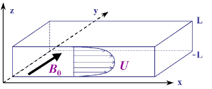
Figure 1: Channel flow under spanwise magnetic field; configuration and computational domain.

In this paper, we consider a channel flow of an incompressible electrically conducting fluid (for example, a liquid metal) driven by a pressure gradient and affected by a uniform steady-state magnetic field oriented in the spanwise direction (see fig. 1). It is assumed that the magnetic Reynolds number is small

$$\mbox{{Re}}_{m}\equiv\frac{UL}{\eta}\ll 1.$$ (1)

Here, $U$ and $L$ are the typical velocity and length scales, chosen in our case as the centerline velocity of the laminar flow and half the channel width, and $\eta=(\sigma\mu_{0})^{-1}$ is the magnetic diffusivity, $\sigma$ and $\mu_{0}$ being the electric conductivity of the liquid and magnetic permeability of vacuum, respectively. The assumption (1) is satisfied by the majority of industrial and laboratory flows of liquid metals. The prominent examples of industrial applications are the continuous casting of steelThomas and Zhang (2001) and growth of large semiconductor crystals by the Czochralski method,von Ammon et al. (2005) where constant magnetic fields are imposed with the purpose of controlling the flow and suppressing unwanted motions. Another example is the liquid metal (Li or Li₁₇Pb) cooling blankets of breeder type for future fusion reactors, where the inevitable and very strong magnetic fields play a negative role by suppressing turbulent heat and mass transfer.Barleon et al. (2001)

The key feature of the low-$\mbox{{Re}}_{m}$ magnetohydrodynamics, which separates it from high-$\mbox{{Re}}_{m}$ plasma and geo- and astrophysical applications, is that the perturbations of the magnetic field induced by fluid motions are much smaller than the imposed magnetic field and can be neglected. One can also assume that the magnetic field perturbations adjust instantaneously to the velocity fluctuations. As a result of these assumptions, the quasi-static approximation Roberts (1967) can be applied, according to which the Lorentz force is expressed as a linear functional of velocity, and the governing equations for fluid motion and electric potential are represented in a closed form as shown in the next section. The flow is characterized by two non-dimensional parameters. The first one is the Reynolds number

$$\mbox{{Re}}\equiv UL/\nu,$$ (2)

while the second is either the Hartmann number

$$Ha\equiv BL(\sigma/\rho\nu)^{1/2}$$ (3)

or the magnetic interaction parameter

$$N\equiv Ha^{2}/Re$$ (4)

characterizing the ratios of Lorentz to viscous and Lorentz to inertia forces, respectively. In the formulas above, $B$ is the strength of the applied magnetic field and $\rho$ and $\nu$ are the density and kinematic viscosity of the fluid.

The transformation of low-$\mbox{{Re}}_{m}$ turbulence under the impact of an imposed uniform steady-state magnetic field has been relatively thoroughly investigated for two simplified flows: homogeneous turbulence and the Hartmann flow. Let us briefly discuss the aspects of the results relevant for our study.

Homogeneous turbulence and its computational counterpart, the flow in a periodic box, are particularly convenient for investigating the basic features of the MHD transformation of turbulent fluctuations far from solid walls. This was done analytically, Moffatt (1967); Davidson (1997); Alemany et al. (1979) numerically, Schumann (1979); Zikanov and Thess (1998); Knaepen and Moin (2004); Vorobev et al. (2005) and experimentally.Alemany et al. (1979) It has been found that the magnetic field affects the flow in two different ways. First, the induced electric currents lead to additional suppression of turbulence via Joule dissipation. Second, the flow acquires anisotropy of gradients. A simple explanation of the origins of the anisotropy is obtained by considering the rate of Joule dissipation

$$\mu(\bm{k})=\sigma B^{2}\rho^{-1}|\hat{\bm{u}}(\bm{k},t)|^{2}\cos^{2}\theta$$ (5)

of the Fourier velocity mode $\hat{\bm{u}}(\bm{k})$, where $\theta$ is the angle between the wavenumber vector $\bm{k}$ and the magnetic field $\bm{B}$. The magnetic field tends to suppress the modes with small values of $\theta$, that is to eliminate velocity gradients along the magnetic field lines. The flow becomes anisotropic and may even approach a two-dimensional state with all fields uniform in the direction of the magnetic field lines in the limit $N\rightarrow\infty$.

The picture described above does not take into account the non-linear interactions that tend to restore the flow isotropy. The interplay between the two opposing effects was investigated numerically, most recently in DNS and LES Vorobev et al. (2005); Vorobev and Zikanov (2008) of forced homogeneous turbulence. Among other results, it has been found that the degree of the anisotropy is a relatively robust function of the magnetic interaction parameter $N$. The influence of the Reynolds number, the type of the large-scale forcing, and, remarkably, the length scale, at which the anisotropy is measured, is weak.

The Hartmann flow, i.e. the flow in a channel with uniform magnetic field imposed in the direction transverse to the channel walls Hartmann and Lazarus (1937) is a classical MHD flow that was the subject of numerous analytical, experimental, and computational investigations such as, e.g. , Refs. Sommeria and Moreau, 1982; Reed and Lykoudis, 1978; Krasnov et al., 2004; Boeck et al., 2007. We would like to stress that, despite the common geometry, there are fundamental differences between the Hartmann flow and the flow studied in the present paper. In the Hartmann channel, the magnetic field interacts directly with the mean flow and changes its profile into the form with nearly flat core and thin Hartmann boundary layers. In our case, no Lorentz force is produced by the interaction between the mean flow and the magnetic field. The MHD effect on the mean flow can, thus, only be indirect, via the transformation of turbulent fluctuations.

In essential aspects of field-flow interaction our configuration is closer to the homogeneous turbulence than to the Hartmann channel flow. In particular, similarly to homogeneous turbulence and in contrast to the Hartmann flow, the leading role is taken by the direct interaction between the field and small-scale structures and the flow is uniform and infinite in the direction of the magnetic field. As a result, many features of the homogeneous MHD turbulence are expected to be observed in our flow. For example, the simple explanation of the origins of the MHD-related gradient anisotropy based on (5) can be extended straightforwardly to our case if one limits the wave vector $\bm{k}$ to streamwise and spanwise components.

In contrast to homogeneous turbulence, the channel flow with spanwise field provides an opportunity of studying the effect of the MHD transformation of small-scale turbulent structures on the mean flow. This phenomenon, undoubtedly playing an important role in low-$\mbox{{Re}}_{m}$ MHD flows, cannot be addressed in the framework of homogeneous turbulence or, in a direct and unequivocal way, of the Hartmann flow. Furthermore, we can investigate the effect of the magnetic field in the presence of a mean shear. This can also be done using the model of a homogeneous shear flow as in Ref. Kassinos et al., 2006, where the case of the moderate magnetic Reynolds number was considered, but the channel provides a more realistic system since it does not require artificial forcing.

In the present paper, we also conduct an a-posteriori verification study of the LES (Large-Eddy-Simulation) models for the case of a channel flow in a spanwise magnetic field. A brief discussion of main known facts concerning the LES modeling of low-$\mbox{{Re}}_{m}$ MHD turbulence is, therefore, in order. The question is closely related to the transformation of turbulent fluctuations discussed above. An accurate LES model must be capable of adjusting to the key effects of the transformation: anisotropy of gradients, suppression of non-linear interactions, steepening of the energy power spectrum, and reduction of the subgrid-scale dissipation rate. Accurate reproduction of the last effect seems particularly important if one takes the view that the primary objective of an LES model is to produce appropriate amount of subgrid-scale dissipation. LES modeling of decaying Knaepen and Moin (2004) and forced Vorobev et al. (2005); Vorobev and Zikanov (2008) homogeneous MHD turbulence provides the basis for an assessment of the performance of Smagorinsky eddy viscosity models. The main conclusion, achieved through comparison with DNS data, is that the classical Smagorinsky model with constant coefficient $C_{S}$ is overdissipative in the MHD case. On the contrary, the model based on the dynamic evaluation of $C_{S}$ Germano et al. (1991); Lilly (1992) has been found to accurately reproduce the reduction of $C_{S}$ and, therefore, of the subgrid-scale dissipation with growing magnetic field and, in general, to give much better agreement with DNS.

LES of the Hartmann flow was conducted using conventional and modified Smagorinsky models,Shimomura (1991) the dynamic Smagorinsky model,Kobayashi (2006); Sarris et al. (2007) and the coherent structure model.Kobayashi (2006) Albeit further studies are needed for more extensive verification farther from the transitional Reynolds numbers, first conclusions can be made. As in the case of the periodic box, the conventional Smagorinsky model becomes highly inaccurate as soon as the flow is significantly affected by the magnetic field. The simple modification based on modeling SGS Joule dissipationShimomura (1991) also does not provide an adequate picture of the flow transformation. The models with coefficients adjustable in accordance to local conditions, such as the dynamic Smagorinsky or coherent structure models, perform much better demonstrating good agreement with DNS and experiments. This is not entirely surprising. The dynamic model has demonstrated its ability to adjust to variations of the dissipation rate on many occasions, including flows with rotation, mean shear, or laminar-turbulent transition.

The only previous work, in which the effect of the spanwise magnetic field on a turbulent channel flow was studied, was the DNS by Lee and Choi.Lee and Choi (2001) Important conclusions were made. In particular, it was found that the imposed spanwise magnetic field suppressed the turbulent fluctuations and reduced the drag. Interestingly, similar behavior was observed for the streamwise magnetic field, but not for the case of Hartmann flow, where suppression of fluctuations was accompanied by increase of drag due to strong shear in the Hartmann boundary layers. It did not take a very strong magnetic field to completely laminarize the flow. For example, in the case of the spanwise field, the laminarization occurred at $N=0.05$.

As will be seen from the following discussion, our results confirm and extend the findings of Ref. Lee and Choi, 2001 An important difference should, however, be noted from the beginning. Due to low numerical resolution and inherent limitations of DNS, the calculations of Ref. Lee and Choi, 2001 were conducted at the low Reynolds number $\mbox{{Re}}\approx 3000$, which is in contrast with $\mbox{{Re}}=10000$ and $20000$ in our work. Furthermore, we conduct a much more detailed analysis of the flow transformation and investigate performance of LES models in the MHD turbulence.

Several experimental studies of turbulent MHD flows in ducts of large aspect ratio with the magnetic field parallel to the longer side were conducted in 1970s. The motivation was essentially the same as of our work: to investigate the effect of the magnetic field on turbulence without the dominating influence of the Hartmann layers. The experiments most relevant to our studyVotsish and Kolesnikov (1977) were performed with a flow of mercury in a rectangular duct of aspect ratio 10 to 1 and values of the Reynolds and Hartmann numbers between 7500 and 15500 and between 0 and 100, respectively. As discussed in detail below, the key experimental results are in good qualitative agreement with our conclusions. We did not attempt to conduct a quantitative comparison. The main reason is that the conditions approaching the ideal configuration of a uniform magnetic field cannot be realized in a straight duct experiment. The magnetic field is inevitably non-uniform in the streamwise direction. Apart from making the quantitative interpretation difficult, this creates the effect of the so-called ‘magnetic obstacle’Votyakov et al. (2007) leading to further deviation between the experimental and numerical data.

The objectives of our study can be summarized as follows. First, we conduct a detailed investigation of the flow transformation caused by the spanwise magnetic field. The change of turbulence statistics, wall friction, and coherent structures is documented and discussed. The second aspect of the motivation concerns the application of LES methods to low-$\mbox{{Re}}_{m}$ MHD turbulence. As discussed above, the dynamic Smagorinsky model has shown reasonably good accuracy in the latter two cases. We present a thorough a-posteriori verification of the model for the case of a channel flow with a spanwise magnetic field.

The paper is organized as follows. A brief review of the computational procedure and LES model is provided in the next section. After presenting the results of the model verification in LES-DNS comparison in section III, we discuss the flow transformation and its anisotropy characteristics in section IV. A discussion of the effect of drag reduction by a spanwise magnetic field and its relation to other mechanisms of drag reduction is given in section V. Finally, concluding remarks are provided in section VI.

II Governing Equations, Numerical Method, and Parameters

II.1 Navier-Stokes equations for low-$\mbox{{Re}}_{m}$ MHD flows

We consider the flow of an incompressible, electrically conducting fluid in an infinite plane channel between insulating walls located at $z=\pm L$, where $x$, $y$ and $z$ denote the streamwise, spanwise and wall-normal directions, respectively (see fig. 1). The flow is driven by a pressure gradient $\partial P_{0}/\partial x$ in the $x$-direction and submitted to a constant spanwise magnetic field $\bm{B}_{0}={B}_{0}\bm{e}$, where $\bm{e}\equiv(0,1,0)$ is the unit vector in the spanwise direction.

In the limit of low magnetic Reynolds number $\mbox{{Re}}_{m}$, the so-called quasi-static approximation Roberts (1967) can be applied. The fluctuating part $\bm{b}$ of the magnetic field due to fluid motion is much smaller than the external magnetic field: $\bm{b}\ll\bm{B}_{0}$. The Lorenz force reduces to

$$\bm{F}=\bm{j}\times\bm{B}_{0},$$ (6)

where the induced electric current density is given by Ohm’s law

$$\bm{j}=\sigma\left(-\nabla\phi+\bm{v}\times\bm{B}_{0}\right).$$ (7)

If displacement currents are neglected and the fluid is assumed electrically neutral, the current density $\bm{j}$ should satisfy the divergence-free constraint $\nabla\cdot\bm{j}=0$. Thus, the electric potential $\phi$ can be expressed via the following equation:

$$\nabla^{2}\phi=\nabla\cdot\left(\bm{v}\times\bm{B}_{0}\right).$$ (8)

The problem is solved in a rectangular domain with periodicity conditions used in the $x$- and $y$-directions following the assumption of flow homogeneity. The no-slip conditions are imposed at the walls:

$$u=v=w=0\hskip 8.53581pt\mbox{at }z=\pm L.$$ (9)

The electric potential $\phi$ is also periodic in the $x$- and $y$-directions. Since no current flows through the electrically insulating walls and the velocity $\bm{v}$ is zero at these walls, (7) leads to the boundary conditions for the electric potential

$$\frac{\partial\phi}{\partial z}=0\hskip 8.53581pt\mbox{at }z=\pm L.$$ (10)

As remarked in section I, in our geometry there is no interaction between the mean flow and the magnetic field. The non-dimensional laminar basic velocity field retains the classical parabolic profile

$$U(z)=1-z^{2}.$$ (11)

Hereafter we use the centerline velocity $U$ of the Poiseuille flow and the half-channel width $L$ as the velocity and length scales correspondingly. Finally, taking the units of the magnetic field and the electric potential as ${B}$ and $LU{B}$, the non-dimensional governing equations and boundary conditions read

$$\frac{\partial\bm{v}}{\partial t}+(\bm{v}\cdot\nabla)\bm{v}=-\nabla p+\frac{1}{Re}\nabla^{2}\bm{v}+N\left(-\nabla\phi\times\bm{e}+\left(\bm{v}\times\bm{e}\right)\times\bm{e}\right),$$ (12)

$$\nabla\cdot\bm{v}=0,$$ (13)

$$\nabla^{2}\phi=\nabla\cdot\left(\bm{v}\times\bm{e}\right),$$ (14)

$$u=v=w=\frac{\partial\phi}{\partial z}=0\hskip 8.53581pt\mbox{at }z=\pm 1.$$ (15)

There are two non-dimensional parameters, the Reynolds number Re and the magnetic interaction parameter $N$, defined in the previous section. To specify the mean pressure gradient we assume that the volume flux $Q$ per span width remains constant.

II.2 Dynamic subgrid scale model

In LES only large and moderate length scales of the flow are resolved. A spatial filtering procedure is applied to the governing equations (12–15), which results in the following equations for filtered fields (denoted by overbar):

$$\frac{\partial\bar{v}_{i}}{\partial t}+\bar{v}_{j}\frac{\partial\bar{v}_{i}}{\partial x_{j}}=-\frac{\partial\bar{p}}{\partial x_{i}}+\frac{1}{Re}\nabla^{2}\bar{v}_{i}-\frac{\partial\tau^{a}_{ij}}{\partial x_{j}}+N\left(-\nabla\bar{\phi}\times\bm{e}+\left(\bar{\bm{v}}\times\bm{e}\right)\times\bm{e}\right)_{i},$$ (16)

$$\nabla\cdot\bar{\bm{v}}=0,$$ (17)

$$\nabla^{2}\bar{\phi}=\nabla\cdot\left(\bar{\bm{v}}\times\bm{e}\right),$$ (18)

$$\bar{v}_{x}=\bar{v}_{y}=\bar{v}_{z}=\frac{\partial\bar{\phi}}{\partial z}=0\hskip 8.53581pt\mbox{at }z=\pm 1.$$ (19)

Here $\tau^{a}_{ij}$ is the traceless part of the sub-grid scale (SGS) stress tensor defined as

$$\tau^{a}_{ij}=\tau_{ij}-\frac{\delta_{ij}}{3}\tau_{kk},\mbox{ with }\tau_{ij}=\overline{v_{i}v_{j}}-\bar{v}_{i}\bar{v}_{j}.$$ (20)

To provide a closure for the filtered equations, the tensor $\tau^{a}_{ij}$ has to be modeled in terms of the resolved fields. The Smagorinsky model is used in the present study. It is based on the eddy-viscosity hypothesis and assumes that

$$\tau^{a}_{ij}=-2\nu_{T}\bar{S}_{ij}=-2C_{S}\bar{\Delta}^{2}|\bar{S}|\bar{S}_{ij},$$ (21)

where $\bar{\Delta}$ denotes the filter width and $C_{S}$ is the Smagorinsky constant. $|\bar{S}|=\left(2\bar{S}_{ij}\bar{S}_{ij}\right)^{1/2}$ is the magnitude of the strain-rate tensor

$$\bar{S}_{ij}=\frac{1}{2}\left(\frac{\partial\bar{v}_{i}}{\partial x_{j}}+\frac{\partial\bar{v}_{j}}{\partial x_{i}}\right).$$ (22)

of the filtered velocity field.

In the classical Smagorinsky eddy-viscosity model, $C_{S}$ is a constant parameter usually adjusted for a particular flow configuration. Germano et al.Germano et al. (1991) proposed an extension to this model, the so-called dynamic procedure, later optimized with a least-square method suggested by Lilly.Lilly (1992) Within this approach, the parameter $C_{S}$ is determined on the basis of the velocity field and, thus, is a function of space and, in general, time. Following the assumption of scale self-similarity of formula (21), the computed velocity field is filtered once again with the so-called “test” filter width $\widehat{\bar{\Delta}}$ larger than the “grid” filter width $\bar{\Delta}$. The spectral cut-off in Fourier space is used in our computations as the filtering operation. No test filtering is performed in the wall-normal direction. The parameter $C(z)$ is determined as

$$C(z)=\frac{<\bar{M}_{ij}\bar{L}_{ij}>_{x,y}}{<\bar{M}_{ij}\bar{M}_{ij}>_{x,y}}$$ (23)

where $\bar{L}_{ij}$ and $\bar{M}_{ij}$ are defined as

$$\bar{L}_{ij}=\widehat{\bar{v}_{i}\bar{v}_{j}}-\hat{\bar{v}}_{i}\hat{\bar{v}}_{j}$$ (24)

and

$$\bar{M}_{ij}=2\bar{\Delta}^{2}\widehat{|\bar{S}|\bar{S}_{ij}}-2\widehat{\bar{\Delta}}^{2}\widehat{|\bar{S}|}\widehat{\bar{S}}_{ij}.$$ (25)

Here symbol $\widehat{...}$ stands for the test filtering, and the spatial averaging over the homogeneous ($x,y$)-directions denoted as $<...>_{x,y}$ is applied to avoid numerical instability. In our simulations, the ratio $\widehat{\bar{\Delta}}/\bar{\Delta}=2$ is used. Further details on the dynamic procedure, its application to classical channel flow, as well as the possible impact of the filter width, can be found in Refs. Germano et al., 1991; Lilly, 1992; Piomelli, 1993.

II.3 Numerical method

The evolution of the flow is found as a numerical solution of the full (12)–(15) or filtered (16)–(19) equations (for DNS and LES parts of our study, correspondingly). We use a pseudo-spectral method, where the flow field is represented by velocity potentials complying with the incompressibility constraint. A detailed description of the algorithm and the corresponding flow solver are given elsewhere.Krasnov et al. (2004, 2008) Briefly, the method applies a Fourier expansion in the horizontal directions, where periodical boundary conditions are imposed, and a Chebyshev polynomial expansion in the vertical direction between insulating walls with no-slip conditions. Nonlinear terms are calculated through Fast Fourier Transforms (FFT). The algorithm is parallelized using domain decomposition in the streamwise direction. FFTs are performed locally by transposition of the data array across the processors.

The modifications made for the present study concern the Lorentz force and the time-stepping method (see also Ref. Krasnov et al., 2008). The Lorentz force term is changed to the case of spanwise orientation of the magnetic field and is now treated as an explicit term in the temporal discretization. Furthermore, the new time-stepping scheme uses three time levels for the approximation of the time derivative and is second-order accurate. We have also implemented de-aliasing following the $2/3$ rule.Canuto et al. (1988) At last, the code now includes the dynamic and conventional Smagorinsky procedures of computation of the SGS stress term $\tau^{a}_{ij}$, so that it can be used both for DNS and LES calculations.

For the conventional Smagorinsky model, the parameter $C_{s}$ in equation (21) is estimated as

$$C_{s}=C^{2}(1-\exp(-z^{+}/25))^{2},$$ (26)

where the value $C=0.1$ found optimal for LES in wall-bounded flows is usedMoin and Kim (1982). The other term is the van Driest damping termvan Driest (1956) for $C_{S}$ near the walls, which is based on the wall distance $z^{+}$ in friction units. To identify the grid filter $\bar{\Delta}$ in that case, we apply the commonly used definition

$$\bar{\Delta}^{3}=\bar{\Delta}_{x}\bar{\Delta}_{y}\bar{\Delta}_{z}.$$ (27)

Here the homogeneous filter widths $\bar{\Delta}_{x}$, $\bar{\Delta}_{y}$ in the horizontal directions and the variable filter width $\bar{\Delta}_{z}$ in the wall-normal are defined as

$$\bar{\Delta}_{x}=\tfrac{3}{2}L_{x}/N_{x},\hskip 14.22636pt\bar{\Delta}_{y}=\tfrac{3}{2}L_{y}/N_{y},\hskip 14.22636pt\bar{\Delta}_{z}^{k}=\tfrac{3}{2}|z_{k-1}-z_{k+1}|/2,$$ (28)

where the collocation points in the Chebyshev direction are denoted by $z_{k}$. The $3/2$ prefactor accounts for the effective number of collocation points due to de-aliasing by the $2/3$-rule.

II.4 Procedure and parameters of numerical experiments

The parameters of the numerical experiments, such as the dimensions of the computational domain, numerical resolution, and Reynolds numbers are listed in Table 1. The simulations were conducted for two values of the constant volume flux identified by the values of the Reynolds number Re based on the half-channel width and centerline velocity of the laminar parabolic profile. The values of the flux-based Reynolds number $\mbox{{Re}}_{q}$ are also given in table 1. The Hartmann number $Ha$ varied between zero and a value close to the threshold above which the three-dimensional turbulence could not be sustained. The flows at higher $Ha$ were characterized by intermittency with long periods of nearly two-dimensional behavior interrupted by three-dimensional bursts. This phenomenon is still under investigation and will not be discussed in the present paper. We only note that the corresponding threshold values of $Ha$ and $N$ seem to depend on the Reynolds number. Continuous turbulence disappears beyond $N\approx 0.09$ for $Re=10000$ and beyond $N\approx 0.08$ for $Re=20000$. For $Re=3000$ studied by Lee & ChoiLee and Choi (2001) the turbulence is already completely suppressed for $N=0.05$. The intermittent dynamics is missing at this value of $Re$ since the laminar state is linearly stable.

The computations were conducted (at given Re and $Ha$) for sufficiently long periods of time until the integral characteristics showed that the statistically steady state was reached. In order to accelerate the evolution of DNS fields, the LES solutions at the same parameters were used as initial conditions. The computations of statistically steady flows were continued for several (not less than 20) convective units $L/U$ and the flow statistics were collected and averaged.

The choice of numerical resolution and domain sizes used for DNS calculations was verified through a comparison with the results by Moser et al.Moser et al. (1999) for non-magnetic turbulent channel flow. The values of $Re_{\tau}$ in our simulations at $Ha=0$ and both Re numbers are very close to those in Ref. Moser et al., 1999 so a detailed comparison between the two studies could be made. In particular, we have analyzed mean velocity profiles and rms values of turbulent fluctuations and found very good qualitative and quantitative agreement.

As an additional verification, we examined two-point correlations and energy spectra of velocity fluctuations for both Re. The two-point correlations computed at $z=0$ in stream- and spanwise directions showed rapid fall-off to nearly zero values at the distance of the half-domain size. The energy spectra were observed to span over $4.5-5$ decimal orders with significant decay at high wavenumbers and without noticeable pile-up at the smallest scales. This demonstrated that the small scales were sufficiently resolved.

The flow solver was also verified in LES computations. In the first series of simulations we examined the effect of LES resolution on convergence of integral flow parameters, such as $Re_{\tau}$ and friction coefficient $C_{f}$. For the test case we used our DNS at $256^{3}$ points and $Re_{\tau}\approx 180$ (corresponding to the turbulent channel flow studied by Kim et al.Kim et al. (1987)) and two LES calculations at $32^{3}$ and $64^{3}$ points employing the dynamic model. The comparison indicated that the LES at $64^{3}$ points almost saturated at the target $Re_{\tau}$ ($178.4$ vs. $180$), whereas the value is clearly underpredicted on the coarser grid ($171.8$ vs. $180$). The latter contributed to approximately $8\%$ difference in the friction coefficient $C_{f}$. Similar dependence of accuracy on numerical resolution was observed earlier by Piomelli et al.Piomelli et al. (1988) with the classical Smagorinsky model at the same $Re_{\tau}$.

We also tested the dynamic model through comparison with the results of channel flow LES at high Reynolds number by Piomelli.Piomelli (1993) Simulations targeting the LES results at $Re_{\tau}=1050$ were conducted for different resolutions ($64^{3}$ and $128^{3}$ points) close to those used in Ref. Piomelli, 1993. The analysis of profiles of mean velocity and rms of turbulent fluctuations as well as the model parameters such as the Smagorinsky constant and SGS stresses $\tau_{ij}$ confirmed proper performance of our LES model.

III DNS vs. LES comparison

In this section we report the results of a-posteriori verification of the dynamic and classical Smagorinsky models conducted via comparison with the data of high-resolution DNS. We also include results of deliberately under-resolved DNS (hereafter UDNS) conducted at the same resolution as the LES runs (see Table 1) but without any SGS terms appearing in the equations. Comparison with UDNS is commonly used in studies of LES models in order to assess the significance of SGS contributions. The assessment becomes even more important in the MHD case because of the possibility indicated by earlier studiesKnaepen and Moin (2004); Vorobev et al. (2005); Vorobev and Zikanov (2008) that at high $Ha$ the MHD flow transformation depopulates the small length scales and reduces their effect on the flow, thus rendering the LES model unnecessary. In such case, the results of UDNS would approach fully-resolved DNS data.

The time-averaged values of the key integral quantities of the flow are listed in table 2. They include the centerline velocity $U_{cl}$, the friction Reynolds number

$$\mbox{{Re}}_{\tau}=\mbox{{Re}}\,u_{\tau},$$ (29)

where the non-dimensional wall friction velocity $u_{\tau}$ is calculated as

$$u_{\tau}^{2}=\mbox{{Re}}^{-1}\left(\partial u/\partial z\right)_{z=-1},$$ (30)

the friction coefficient

$$C_{f}=2(u_{\tau}/U_{q})^{2},$$ (31)

where $U_{q}$ is the flux (mean) velocity, and the volume-averaged dissipation rate at the resolved scales

$$\epsilon=\langle 2\mbox{{Re}}^{-1}S_{ij}S_{ij}\rangle_{v}.$$ (32)

The dissipation rate can be used to assess the importance of the model component in LES since the difference between the DNS and LES values may serve as an approximate measure of the dissipation provided by the SGS closure. One can see that, despite the relatively high numerical resolution of our LES runs, the subgrid-scale dissipation constitutes a significant fraction of the total, especially at the resolution of $64^{3}$ at $\mbox{{Re}}=20000$. The under-resolved DNS produce significantly stronger dissipation, which can be viewed as a result of energy pile-up at the scales near the grid cut-off scale. As expected, the difference between UDNS and DNS decreases with $Ha$, but remains large even at the strongest magnetic fields used in our study.

The data for the centerline velocity $U_{cl}$ show fairly good agreement between the DNS and LES results in all cases and do not allow us to differentiate between the dynamic and classical models. Clear differentiation can, however, be made on the basis of computed $\mbox{{Re}}_{\tau}$ and $C_{f}$. With the possible exception of the case $\mbox{{Re}}=20000$, $Ha=0$, the dynamic model consistently provides values that are closer to the DNS data. The improvement furnished by the dynamic mechanism is particularly significant in the experiments conducted at the lower resolution $64^{3}$ at $\mbox{{Re}}=20000$ (the rows marked as DSM64 and SM64 in table 2). The values of all these coefficients are consistently overpredicted by UDNS. Similarly to the dissipation rate, the error decreases with Ha, but remains significant.

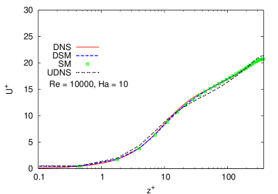
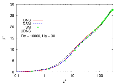
Figure 2: Comparison between the LES and filtered DNS results. Mean velocity profiles in wall coordinates based on $u_{\tau}$ and $\nu$ for $Re=10000$ at $Ha=10$ (left) and $Ha=30$ (right). The results of unresolved DNS (indicated as UDNS) are shown for comparison.

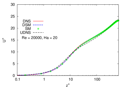
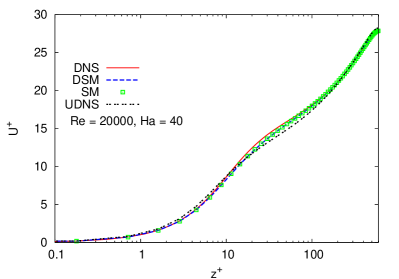
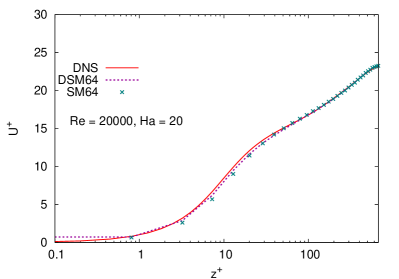
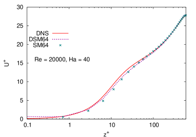
Figure 3: Comparison between the LES and filtered DNS results. Mean velocity profiles in wall coordinates based on $u_{\tau}$ and $\nu$ for $Re=20000$ at $Ha=20$ (left) and $Ha=40$ (right). The results of unresolved DNS (UDNS on top figures) are shown for comparison.

The time-averaged mean velocity profiles are shown in figures 2 and 3 for $\mbox{{Re}}=10000$ & $20000$ and two values of the Hartmann number. Wall units are used and, for the sake of comparison, the DNS velocity field is filtered to the LES resolution using the spectral cut-off operation. One can see that both the dynamic and the classical models accurately reproduce the DNS profile. The difference between the two models becomes more visible if the resolution is lowered to $64^{3}$. The results presented by the bottom pictures of figure 3 show that the classical model poorly reproduces the buffer region, especially for the case of higher $Ha$. As illustrated by the top pictures of figure 3, the UDNS fails to reproduce the entire velocity profile in the whole range of Re and $Ha$ numbers. At $\mbox{{Re}}=20000$, the $64^{3}$ simulation using the dynamic model produces better results than UDNS at the resolution $128^{3}$.

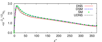
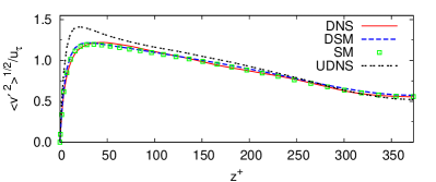
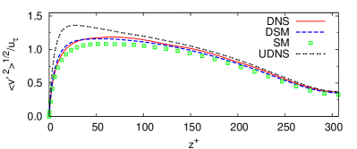
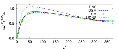
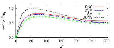
Figure 4: Comparison between the LES and filtered DNS results. Horizontally and time-averaged turbulence intensities in wall coordinates for $Re=10000$ at $Ha=10$ (left) and $Ha=30$ (right). Root mean square of velocity fluctuations scaled by DNS wall shear velocity (30) are shown. The results of unresolved DNS are also shown (UDNS).

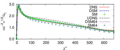
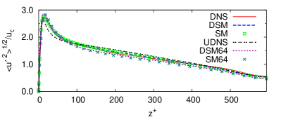
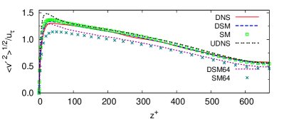
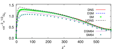
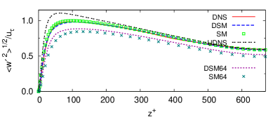
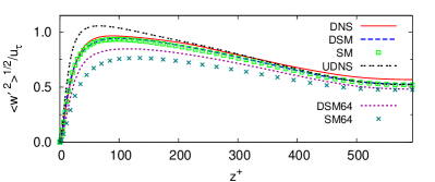
Figure 5: Comparison between the LES and filtered DNS results. Horizontally and time-averaged turbulence intensities in wall coordinates for $Re=20000$ at $Ha=20$ (left) and $Ha=40$ (right). Root mean square of velocity fluctuations scaled by DNS wall shear velocity (30) are shown. The results of unresolved DNS are also shown (UDNS).

The typical results for the DNS – LES comparison of the turbulence intensities are shown in figures 4 and 5. Horizontally- and time-averaged profiles of the rms of fluctuations of streamwise ($u^{\prime}$), spanwise ($v^{\prime}$), and wall-normal ($w^{\prime}$) velocity components are plotted for $\mbox{{Re}}=10000$ at $Ha=10$ and $30$ (fig. 4) and $\mbox{{Re}}=20000$ at $Ha=20$ and $40$ (fig. 5). The scaling by the DNS wall shear velocity is applied to all data. One can see that the intensity of the streamwise fluctuations is well reproduced by both LES models. The situation is different in the cases of spanwise and wall-normal components. Here, the classical Smagorinsky model underestimates the fluctuation intensities at high Hartmann number, while the dynamic model remains reasonably accurate. The results for $\mbox{{Re}}=20000$ at resolution $128^{3}$ demonstrate better agreement between the DNS and LES without clear prevalence of any model. This situation changes for the lower resolution, in which case the dynamic model shows better performance than its classical counterpart. The under-resolved DNS gives reasonably accurate results for the streamwise intensities but severely overestimates intensity of fluctuations of the spanwise and wall-normal components.

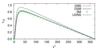
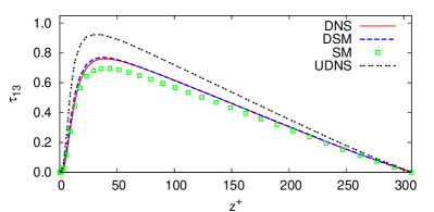
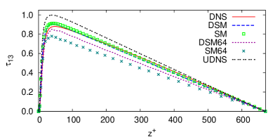
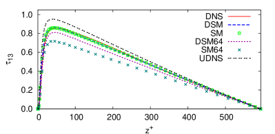
Figure 6: Comparison between the LES and DNS results. Horizontally and time-averaged Reynolds shear stress $\tau_{13}$ in wall coordinates for $Re=10000$ (top) at $Ha=10$ (left) and $Ha=30$ (right) and for $Re=20000$ at $Ha=20$ (left) and $Ha=40$ (right). Unfiltered DNS, UDNS, and full LES ($\tau_{\textrm{\tiny resolved}}$ + $\tau_{\textrm{\tiny SGS}}$) stresses are shown. Normalization is by $u^{2}_{\tau}$ obtained for each case from DNS.

The profiles of time-averaged Reynolds shear stresses $\tau_{13}=\langle u^{\prime}w^{\prime}\rangle$ are shown in figure 6. The unfiltered velocity field is used to compute $\tau_{13}$ in DNS and UDNS, while the sum of computed $\tau_{resolved}$ and modeled $\tau_{SGS}$ components represents the LES solution. The data for $\mbox{{Re}}=10000$ and $Ha=10$, $30$ and for $\mbox{{Re}}=20000$ and $Ha=20$, $40$ are presented. In each case, the curves are normalized by $u^{2}_{\tau}$ taken from the DNS solution. The comparison between the DNS and LES curves shows higher accuracy of the dynamic model, which becomes obvious when the data for higher Hartmann numbers or for lower numerical resolution (at $\mbox{{Re}}=20000$) are considered. It is clear that the conventional Smagorinsky model underestimates the shear stress, whereas UDNS yields significant over-estimation.

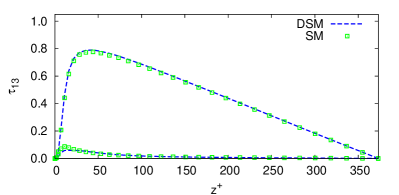
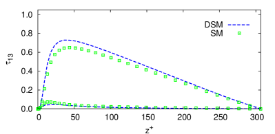
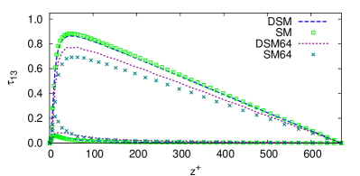
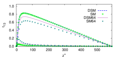
Figure 7: Separate contributions of the resolved $\tau_{\textrm{\tiny resolved}}$ (upper curves) and subgrid $\tau_{\textrm{\tiny SGS}}$ (lower curves) stresses in LES simulations. Horizontally and time-averaged Reynolds shear stress $\tau_{13}$ in wall coordinates for $Re=10000$ (top) at $Ha=10$ (left) and $Ha=30$ (right) and for $Re=20000$ at $Ha=20$ (left) and $Ha=40$ (right). Normalization is by $u^{2}_{\tau}$ obtained for each case from DNS.

Figure 7 shows separate contributions from the resolved $\tau_{resolved}$ and the modelled $\tau_{SGS}$ stresses. Apart from presenting the relative roles played by the resolved and modeled parts of the turbulent momentum transfer, the curves illustrate difference between the dynamic and classical Smagorinsky models. The two models generate close results in the high-resolution LES. In the case of the low-resolution LES, the contribution of the modeled stresses is higher for the classical model. Correspondingly, the resolved stresses are lower than for the dynamic model. Considering the effect of the magnetic field, it is interesting to note that stronger field does not result in preferential suppression of the SGS stress component. Both components are visibly reduced (this phenomenon is discussed in the following section).

We can now formulate conclusions regarding the performance of the classical and dynamic Smagorinsky models. The models perform significantly better than simple underresolved DNS. Both models are reasonably accurate in reproducing the mean flow. The same is true for the intensities of turbulent fluctuations, although the classical model shows a tendency toward underestimation of the normal and spanwise components at high Hartmann numbers. The real difference between the models becomes visible when we consider the characteristics of the momentum transfer in the wall-normal direction, such as the Reynolds shear stress $\tau_{13}$, wall shear Reynolds number $\mbox{{Re}}_{\tau}$, or the friction coefficient $C_{f}$. For all these characteristics, the dynamic model consistently generates significantly more accurate results.

IV Flow transformation caused by the magnetic field

This section presents the results of a systematic study of the effects of the spanwise magnetic field on the flow properties. Since the accuracy of the dynamic Smagorinsky model has been proven for the set of parameters under consideration in the previous section, the data from DNS and dynamic LES will be used interchangeably. Table 2 summarizes the parameters and computed integral characteristics of all numerical experiments.

IV.1 Integral characteristics

As already noted by Lee & ChoiLee and Choi (2001) and confirmed by the results of our computations presented below, the spanwise magnetic field tends to suppress the turbulent fluctuations and turbulent momentum transfer in the wall-normal direction. The integral effect is a reduced friction drag. This also leads to a smaller slope of the velocity profile near the wall. The centerline velocity should increase to maintain the constant volumetric flux.

While all this can be inferred from table II, it is nonetheless instructive to present this information graphically. Figs. 8(a,b) show the centerline velocity and the relative friction coefficient $C_{f}/C_{f}(Ha=0)$ as functions of the magnetic interaction parameter $N$ for the two different Reynolds numbers. We see that the centerline velocity increases monotonously with $N$ and that the data sets for the different Reynolds numbers are fairly close.

The same observation applies for the normalized friction coefficient, which decreases almost linearly with $N$. The friction coefficient is reduced about 30 percent before the sustained turbulence is replaced by intermittent dynamics.

We finally note that by comparison with the laminar state the drag reduction is rather modest. The laminar friction coefficient is $C_{f}=0.00090$ for $Re=10000$ and $C_{f}=0.00045$ for $Re=20000$, i.e. it is almost an order of magnitude smaller than for the turbulent states obtained in our simulations.

IV.2 Mean profiles

Figure 9 shows the profiles of time-averaged mean velocity $U=\langle u\rangle$ as obtained in DNS. In figures 9(a,b), the global coordinates are used and the velocity is scaled with the flux velocity $U_{q}$. One can see that the mean flow profile changes significantly as the magnetic field becomes stronger (the Hartmann number grows). The transformation resembles a ‘transition’ towards the laminar profile, with the centerline velocity growing and the gradient near the wall decreasing. As shown below, this does not mean actual laminarization – the flow remains fully turbulent. Similar behavior was observed in the duct flow experiment of Ref. Votsish and Kolesnikov, 1977.

In general, there is no reason why the logarithmic layer behavior should not be observed in the MHD channel flow with spanwise magnetic field. The Lorentz force does not directly appear in the equation for wall-normal transport of mean momentum. The dimensional arguments leading to the log-layer solution should remain valid provided, of course, the flow retains the pattern of inner, outer, and overlap sub-layers. On the other hand, the magnetic field affects the solution indirectly, by transforming the turbulent fluctuations and, thus, the turbulent momentum transport by $\tau_{13}$.

Our attempt to identify the log-layer behavior is illustrated in figure 9. The DNS mean velocity profiles are plotted in wall units in figures 9(c,d). It is difficult to make a definite conclusion but one may convince oneself upon observation that the profiles contain intervals of nearly logarithmic behavior. This conclusion would be wrong as illustrated in figures 9(e,f), where the profiles of compensated velocity gradient $\gamma\equiv z^{+}du^{+}/dz^{+}$ are shown. Such profiles were used in the past (for example, in Ref. Moser et al., 1999) to assess the agreement between the computed data and the log-law, according to which the inverse von Kármán constant $\kappa$ equals $\gamma$. One can see in figure 9 that the logarithmic layer is absent in the flows affected by the magnetic field. This is observed for all non-zero Hartmann numbers considered and for both values of the Reynolds number. We also tried to identify possible power law behavior $u^{+}\sim(z^{+})^{n}$ suggested in Ref. Barenblatt et al., 1997. After considering the compensated profiles $\beta\equiv z^{+}(u^{+})^{-1}du^{+}/dz^{+}$, we found a situation similar to that of the log-layer. $\beta$ was nearly constant in an extended range of $z^{+}$ for non-magnetic flows (see Ref. Moser et al., 1999 for similar results) but not for the flows in the presence of the magnetic field.

The effect of the magnetic field on the turbulent velocity fluctuations is illustrated in Figure 10. Time-averaged profiles of root mean square fluctuations for each velocity component and of full (resolved plus SGS) turbulent shear stress $\tau_{13}$ are shown as found in dynamic Smagorinsky LES. For the purpose of comparison of the absolute magnitudes, the common velocity scale, namely the flux velocity $U_{q}$ is used for normalization. The main conclusion is in agreement with the DNS results of Lee and ChoiLee and Choi (2001) and with the experimental data.Votsish and Kolesnikov (1977) The magnetic field suppresses the turbulent fluctuations. The degree of suppression grows monotonically with the strength of the magnetic field and is somewhat larger for the wall-normal velocity component than for the other two. An important consequence is the substantial reduction of the turbulent shear stress illustrated by figures 10(g,h). The resulting decrease of the turbulent momentum transfer in the wall-normal direction is, obviously, a reason for the transformation of the mean flow profile shown in figure 9 and for the drag reduction. Interestingly, the suppression of turbulent fluctuations is not accompanied by any noticeable change of the global spatial structure of the flow. In particular, the dimension of the viscous sublayer and locations of the maxima of the fluctuation energy and turbulent stress are unaffected by the magnetic field.

IV.3 Coherent structures

In this part of the paper, we analyze the effect of the spanwise magnetic field on the flow structures. The study of such structures in the homogeneous MHD turbulenceZikanov and Thess (1998); Vorobev et al. (2005); Knaepen and Moin (2004); Kassinos et al. (2006) proved quite fruitful. It was found that a sufficiently strong magnetic field transforms the velocity and vorticity field in a unique and clearly visible way. The main feature of the transformation is growth of the typical size of the coherent structures, strong in the direction of the magnetic field and weaker, but noticeable in the transverse directions. In general, the structures become larger, slower, and less intense.

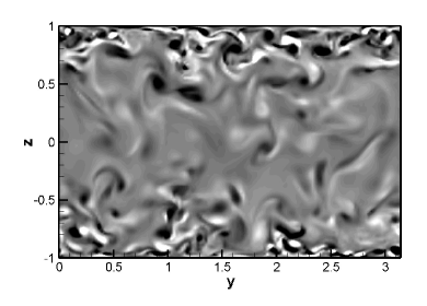
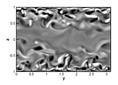
(c)

(d)

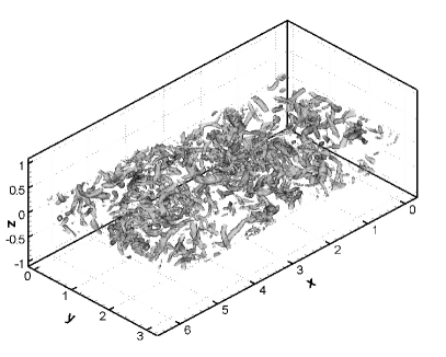
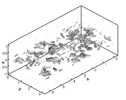
(e)

(f)

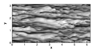
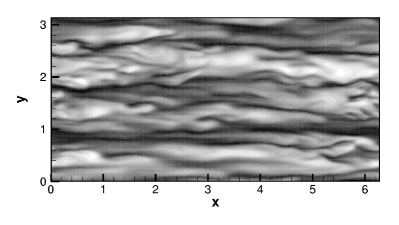
Figure 11: Effect of magnetic field on coherent structures of the flow. Results of DNS are shown for $\mbox{{Re}}=10000$ and $Ha=0$ (a,c,e) and $Ha=30$ (b,d,f). All fields are normalized by the corresponding rms values. (a,b), Contour plots of streamwise vorticity in the transverse plane. (c,d), Iso-surfaces $\lambda_{2}=-0.1$ shown in the middle of the channel at ($-0.25<z<0.25$). (e,f), Contour plots of the streamwise velocity fluctuations at $z=0.95$.

The situation in the channel flow is more complex, in particular, due to the obvious difference between the core flow and the boundary layers. In the core, where the mean shear is weak, a transformation similar to that in homogeneous turbulence can be expected. On the contrary, in the boundary layers, the evolution of the coherent structures is dominated by the mean shear and the effect of the magnetic field can be quite different. The results of our calculations, illustrated in figure 11, largely meet these expectations. To identify the coherent structures, we analyzed the fields of streamwise vorticity $(\bm{\nabla}\times\textbf{u})_{x}$, fluctuations of streamwise velocity $u^{\prime}$, and the intermediate eigenvalue $\lambda_{2}$ of the tensor $S_{ik}S_{kj}+\Omega_{ik}\Omega_{kj}$, where $S_{ik}\equiv(v_{i,k}+v_{k,i})/2$ and $\Omega_{ik}\equiv(v_{i,k}-v_{k,i})/2$.

The contour plots of the streamwise vorticity component in the plane perpendicular to the direction of the channel are shown in figures 11(a,b). The vorticity field is scaled by its root mean square value in each case. Near the walls, the regions of localized strong vorticity become somewhat larger in the presence of the magnetic field. Similar behavior was observed by Lee and Choi,Lee and Choi (2001) although in their case, the transformation was more pronounced due to lower Reynolds number and numerical resolution. The effect of the magnetic field is stronger in the middle part of the channel, where the structures seem to be suppressed to a larger degree than near the walls. In general, the vorticity magnitude decreases as can be seen from comparison of the rms values $\langle\omega_{x}^{2}\rangle^{1/2}=1.643$ at $Ha=0$ and $1.022$ at $Ha=30$.

The connected regions of negative $\lambda_{2}$ eigenvalue are often considered as indicators of coherent vortical structuresJeong and Hussein (1995) especially in the regions of strong mean shear. Our analysis of the $\lambda_{2}$ fields led to the same conclusions as based on the vorticity field. As an illustration, the figures 11(c,d) show the isosurfaces $\lambda_{2}=-0.1\lambda_{2,rms}$ in the middle part of the channel. One can see that the structures decrease in number, increase in size, and, seemingly, become elongated in the direction of the magnetic field. The latter observation will be confirmed below by quantitative characteristics of the flow anisotropy.

The effect of the magnetic field on near-wall streaks is illustrated in figures 11(e,f), where the contours of streamwise velocity perturbations at $z=0.95$ are shown. The fields are normalized by their rms values averaged over the horizontal plane. This should not obscure the fact that, as illustrated in figure 10a, the amplitude of the streaks is lower at $Ha=30$. As can be seen in figures 11(e,f), they also become more stable (less susceptible to small-scale perturbations) and wider in the spanwise direction. These observations are also in agreement with the earlier results by Lee and Choi.Lee and Choi (2001)

IV.4 Anisotropy

Discussing the flow anisotropy we should clearly separate the following two types: the anisotropy of dimensionality referring to variation of the typical length scale with direction, and the anisotropy of componentality, which means imparity between the velocity components and can be viewed as anisotropy of the Reynolds stress tensor (see Ref. Kassinos et al., 2001 for a discussion of terminology). Both types are present in the channel flow. The focus of our study is, however, on the dimensionality anisotropy, since only this type is affected by the magnetic field directly.

The question of anisotropy in the combined presence of mean shear and magnetic field is non-trivial. We deal with two competing effects, each leading to establishment of its own anisotropy. The mean shear promotes elongation and alignment of flow structures in the streamwise direction, while the magnetic field produces similar (in effect but not in mechanism) action along the magnetic field lines, i.e. in the spanwise direction. The situation was considered earlier for the case of homogeneous turbulence.Kassinos et al. (2006) The DNS computations in a periodic box confirmed the predictions based on an analysis of the typical time scales. The two relevant scales are the typical shear time $\tau_{S}=S^{-1}$, where $S$ is the mean shear rate, and the Joule damping time $\tau_{J}=\rho/\sigma B^{2}$. It was foundKassinos et al. (2006) that at low magnetic Reynolds number the type of the anisotropy is determined by the ratio $M\equiv\tau_{S}/\tau_{J}=\rho^{-1}B^{2}\sigma S^{-1}$. The flow structures elongate with the mean shear at $M\ll 1$ and with the magnetic field at $M\gg 1$.

We evaluated the parameter $M$ as a function of the wall-normal coordinate $z$ using the local magnitude of the derivative of the mean velocity $U$. In our units, the parameter is defined as $M=N\left(dU/dz\right)^{-1}$. It was found that the condition $M\ll 1$ is satisfied in a larger part of the channel in all our experiments. At the highest interaction parameter $N=0.09$ corresponding to $\mbox{{Re}}=10000$ and $Ha=30$, $M$ was below 0.1, 0.25, and 0.5 at $|z|\gtrsim 0.85$, 0.5, and 0.1, respectively. This means that the anisotropy properties are predominantly controlled by the mean shear with exception of the region in the middle of the channel. The visualizations of the flow structures presented above provide certain support to this conclusion. A more quantitative assessment is provided in what follows.

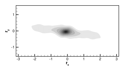
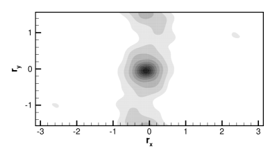
(c)

(d)

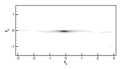
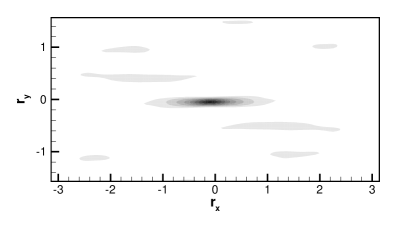
Figure 12: Effect of magnetic field on flow anisotropy. Contour plots of the correlation coefficient (33) for the streamwise velocity component computed for the DNS fields at $\mbox{{Re}}=10000$ $Ha=0$ (a,c) and $Ha=30$ (b,d) are shown in the middle of the channel at $z=0$ (a,b) and near the wall at $z=0.95$ (c,d).

The typical results for the two-point correlations are presented in figure 12. The correlations were calculated for the streamwise velocity component as

$$C=\frac{\langle u(\textbf{x}+\textbf{r})u(\textbf{x})\rangle}{\langle u(\textbf{x})^{2}\rangle},$$ (33)

where x stands for the physical coordinates and $\textbf{r}=(r_{x},r_{y},0)$ is the horizontal displacement vector, and the averaging is done over a horizontal plane. No time averaging is applied to the correlation coefficients. The results for the flow without magnetic field and for the flow with the highest magnetic interaction parameter $N=0.09$ are shown in figures 12(a,c) and 12(b,d), respectively. In the middle of the channel (see figures 12(a,b)), the effect of the magnetic field is to extend the correlations in the spanwise direction. The effect of the magnetic field is not very strong and concerns primarily the weak correlation ranges. In the area of strong mean shear near the walls (see figures 12(c,d)), the effect of the magnetic field is also visible. The degree of correlation increases in the streamwise and spanwise directions. This is in agreement with the conclusion made on the basis of visualization of the same flow fields in figures 11(e,f), and which will be further confirmed below. It can also be noticed that the ratio of the typical correlation lengths in the two directions is not affected by the magnetic field.

The anisotropy of dimensionality can be viewed as anisotropy of the velocity gradients. This viewpoint seems particularly attractive in the case of the low-$\mbox{{Re}}_{m}$ MHD turbulence, where the mechanism of anisotropy generation is the preferential suppression of flow modes with strong gradients along the magnetic field lines. A natural way to evaluate such anisotropy is to use the ratios of the mean square velocity gradients

$$G_{ij}=\frac{\langle\left(\partial v_{i}/\partial y\right)^{2}\rangle\left(1+\delta_{i2}\right)}{\langle\left(\partial v_{i}/\partial x_{j}\right)^{2}\rangle\left(1+\delta_{ij}\right)}.$$ (34)

Here $y$ is the coordinate in the direction of the magnetic field. The factors in the numerator and denominator are introduced so that each coefficient $G_{ij}$ varies between 0 in a purely two-dimensional flow, which is uniform in the $y$-direction and 1 in a perfectly isotropic flow.

The coefficients (34) were successfully used in the numerical studies of turbulence in a periodic box.Schumann (1979); Zikanov and Thess (1998); Vorobev et al. (2005) One of the reasons is that in such flows the degree of anisotropy is nearly scale-independent in a wide range of intermediate and small scales.Vorobev et al. (2005) The dominant contribution by the intermediate scales makes the coefficients (34) convenient and fairly accurate measures of anisotropy in this range,Vorobev et al. (2005) which, importantly for the LES modeling, includes the typical scales of filtering. This property was employed in Ref. Vorobev and Zikanov, 2008, where a simple anisotropy correction of the classical Smagorinsky model based on computed values of $G_{ij}$ was proposed and verified.

The channel flow is a more complex and less straightforward subject of the analysis in terms of $G_{ij}$ than the flow in a periodic cube. The major complicating factor is the presence of the mean shear that creates the anisotropy of a different orientation. It also leads to spatial non-uniformity. The situation in the core flow is clearly different from that near the walls. Furthermore, one may expect the behavior of the coefficients to vary depending on the choice of the velocity component $v_{i}$. Keeping these difficulties in mind, we conduct the analysis of the $G_{ij}$ coefficients in the rest of this section.

The coefficients are calculated as functions of $z$ using horizontal and time-averaging as a substitute to the volume averaging employed in the periodic box flows. The values of the mean square of velocity gradients $\langle\left(\partial v_{i}/\partial x_{j}\right)^{2}\rangle$ obtained in DNS and LES differ significantly from each other, which indicates substantial contribution of the subgrid scales. The same effect was illustrated in table 2 on the example of the dissipation rate. The agreement between the LES and filtered DNS is quite good. Unlike the case of periodic box flows, the ratios of the gradients, i.e. the coefficients (34) are also noticeably different between DNS and LES, especially for the coefficients that include $x$-derivatives. This can be attributed to the scale-dependent character of the anisotropy generated by mean shear. Only the DNS data are presented and discussed below.

The results for $\mbox{{Re}}=10000$ are shown in figure 13. Similar behavior was detected in the runs with $\mbox{{Re}}=20000$. The ratios of the spanwise and normal derivatives are plotted in figures 13(a-c) (the top row). One can clearly see the effect of the magnetic field in the middle of the channel. The perturbations are nearly isotropic in the $y-z$ plane at $Ha=0$. As the Hartmann number increases, the growing suppression of the spanwise derivatives by the magnetic field results in consistent decrease of the coefficients. The effect of the magnetic field becomes negligible near the walls, where the behavior of all coefficients is nearly identically dominated by the growing normal derivatives.

The streamwise and normal derivatives, ratios of which are plotted in figures 13(d-f) (the middle row), show anisotropy created by the mean shear at $Ha=0$. According to the commonly known picture, the flow structures are characterized by weaker gradients (slower variation) in the streamwise than in the spanwise direction. It is interesting that the magnetic field enhances this anisotropy. The effect of growing Hartmann number is obvious and unambiguous. It is also quite remarkable since neither streamwise nor normal derivatives are directly affected by the magnetic field.

The last row of figure 13 shows the ratios of streamwise and spanwise derivatives. Here, again, we see the coefficients decreasing near the wall, which is a consequence of the dominance of streaky structures. Regarding the effect of the magnetic field, one could expect that, due to direct suppression of the spanwise derivatives, the coefficients would grow with the Hartmann number. The figures 13(g-i) prove such expectations wrong. First, the coefficients do not change significantly at all. Second, they, in fact, decrease with $Ha$. This occurs for all three velocity components throughout the channel except in the very central part of it for the coefficients based on $u$ and $w$. We see that the magnetic suppression of spanwise derivatives is accompanied by stronger reduction of the streamwise ones.

An alternative measure of the deviations from local isotropy (or of anisotropy) is the skewness of the transverse derivative of the streamwise velocity fluctuations which is defined as

$$S_{3}(z)=\frac{\langle(\partial u/\partial z)^{3}\rangle}{\langle(\partial u/\partial z)^{2}\rangle^{3/2}}\,,$$ (35)

where the statistical averages are taken in $x,y$-planes at fixed height $z$. This ratio has been succesfully applied to measure the return of shear flow turbulence to a state of local isotropy in the presence of a large-scale source of anisotropy, the sustained mean flow. Warhaft (2002); Gualtieri et al. (2002); Schumacher et al. (2003) In a perfectly isotropic flow, all odd-order moments have to be zero. Note that a non-vanishing skewness profile has to reverse sign at the midplane for symmetry reasons in our case.

A positive derivative skewness over the half-channel ($z\in[-1,0]$) is observed in Fig. 14 for all four cases. The profiles indicate that positive gradients are more likely than negative ones. In other words, the streamwise velocity fluctuations increase preferentially with growing $z$. It can be observed that magnitude in both non-magnetic cases decreases slightly with increasing Reynolds number, thus indicating that a return to local isotropy which states that a growing range of small scales is less affected by the presence of the global shear. The rapid increase of all profiles close to the wall is a fingerprint of the streamwise streaky structures that are formed. The figures also display that a less rapid increase of the skewness profile is in line with less rapid decrease of the local mean shear or the thickening of the viscous layer. All profiles decrease then to zero at the midplane.

The strongest suppression of the turbulent fluctuations and the preferential alignment with the mean flow becomes clearly visible in the case of $Re=20000$ and $Ha=40$ in comparison to both, the $Ha=0$ case at the same Reynolds number and the $Ha=30$ case at the lower Reynolds number of 10000. The findings are consistent with the more pronounced streamwise structures which are displayed in Fig. 11(e) compared to (f). We can conclude that the drag reduction goes in line with a larger amplitude of the derivative skewness. The spanwise magnetic field reduces the degree of local isotropy which is also consistent with the trends of the profiles in Fig. 13.

We now can summarize the results of our study of the dimensionality anisotropy in the MHD channel flow. The picture of strong anisotropy induced by the magnetic field in simulations of homogeneous (periodic box) turbulenceSchumann (1979); Zikanov and Thess (1998); Knaepen and Moin (2004); Vorobev et al. (2005) cannot be directly translated to the channel case. The anisotropy properties remain predominantly determined by the mean shear, especially in the wall regions. The main effect of the magnetic field is to reduce the velocity gradients in both horizontal directions. We can view this as another manifestation of the phenomenon already observed in the visualization of the coherent structures, namely growth of typical spanwise and streamwise length scales.

V Comparison with drag reduction by stratification and polymer additives

The results in Table 2 show that the spanwise magnetic field results in noticeable reduction of the friction drag. It is interesting to relate the present mechanism of drag reduction to other known mechanisms. In this section, we do so for two cases: channel flow in the presence of stable stratification and channel flow with minute amounts of long flexible polymer chains added. In particular, we seek to identify the similarities and differences in the momentum flux balance for both types of flows and to rationalize the resulting differences in the mean profiles.

The turbulent channel with stable density stratification in the wall-normal direction was a subject of a detailed LES studyArmenio and Sarkar (2002). The strong effect on the momentum transfer and the mean flow was observed, which, albeit caused by a different mechanism, is similar to the effect of the magnetic field detected in the present study. In particular, increase of the Richardson number led to growing suppression of turbulent fluctuations and reduction of wall-normal turbulent momentum flux $\tau_{13}$. The transformation of the mean velocity profile visually similar to that shown in our figures 9a,b was found. In contrast to the case with the magnetic field, the stratification was reported to retain the logarithmic layer behavior. On the other hand, the details of the transformation of the log-layer, such as increased slope, reduced intercept, and widened zone of the core flow, were consistent with our observations.

The phenomenon of polymer drag reduction has been observed in the late 1940ies by TomsToms (1949) and studied well in experimentsVirk (1975); Warholic et al. (1999) and DNS.Sureshkumar et al. (1997); Dimitropoulos et al. (2005); Peters and Schumacher (2007) Dilute polymer solutions are modeled as two-component fluids, where stresses of the Newtonian solvent and polymer component are additive. The simplest additional macroscopic stress field is given by

$$\tau_{ij}^{(p)}({\bf x},t)=\frac{\eta_{p}}{\lambda}(fC_{ij}-\delta_{ij})\,.$$ (36)

Here, $\eta_{p}$ is the dynamic polymer viscosity (depending on polymer concentration), $\lambda$ the characteristic relaxation time of the macromolecule chains, $f=f(|{\bf R}|)$ the dimensionless Peterlin function which reflects the finite extensibility of the chains. The components of the end-to-end vector of an ensemble of polymer chains, ${\bf R}$, are combined to a macroscopic dimensionless conformation tensor $C_{ij}$ by a dyadic product. The streamwise component of the Reynolds equation obtained after an integration with respect to $z$ and horizontal averaging is given by

$$-\langle u^{\prime}w^{\prime}\rangle(z)+\nu\frac{dU}{dz}+\frac{\nu_{p}}{\lambda}\langle fC_{xz}\rangle(z)=\frac{\tau_{w}}{\rho}\,$$ (37)

in dimensional form, where $\tau_{w}$ is the wall-shear stress. The polymer chains are assumed to be significantly extended beyond their equilibrium extension. Following Benzi et al.,Benzi et al. (2006) the unknown polymer stress term can be closed to

$$\langle fC_{xz}\rangle(z)\approx\lambda\frac{dU}{dz}\langle C_{zz}\rangle(z)\,,$$ (38)

which gives

$$-\langle u^{\prime}w^{\prime}\rangle(z)+[\nu+\nu_{p}\langle C_{zz}\rangle(z)]\frac{dU}{dz}\approx\frac{\tau_{w}}{\rho}\,.$$ (39)

DNS in Ref. Benzi et al., 2006 also suggest that $\langle C_{zz}\rangle(z)\sim z$ close to the wall and $\langle C_{zz}\rangle(z)\sim const$ in the logarithmic layer. This causes a linearly increasing effective viscosity in the viscous layer and a constant but larger one in the logarithmic layer. Drag reduction seems to be associated with the growth of the viscous layer and transition to the logarithmic scaling at larger $z^{+}$ with nearly the same von Kármán constant $\kappa$.

In contrast, the Reynolds stress balance for the magnetic case remains unchanged in comparison to the pure hydrodynamic case, i.e., no additional stress term appears. The spanwise magnetic field provides a turbulent kinetic energy sink that reduces the turbulent velocity fluctuations over the entire width of the channel (see figures 10(g,h)) and does not contribute as a $z$-dependent effective viscosity. This seems to be the only feature separating the MHD case from other flows with drag reduction effects. It can explain why we do not observe growth of the viscous layer as for turbulent polymer solutions. The absence of such growth is clearly seen, for example, in the Reynolds stress profiles in Figs. 10(g,h), which display no shift of the position of the maximum.

The suppression of turbulent energy and the associated reduction of the turbulent momentum transfer in the wall-normal direction also explains the steepening of the mean flow profiles seen in figures 9(a,b). At last, the weakening of the wall-normal momentum transfer can be identified as the mechanism leading to the drag reduction in our flow.

VI Conclusions

In this paper, we presented the results of a detailed investigation of a turbulent channel flow affected by a uniform spanwise magnetic field. The case of low magnetic Reynolds number and electrically insulating walls was considered. Numerical simulations, both DNS and LES, were conducted for two relatively large values of the hydrodynamic Reynolds number and Hartmann numbers in the range from zero to the threshold values above which statistically steady three-dimensional turbulence could not sustained.

A-posteriori comparison between the results of DNS and LES computations demonstrated the ability of the dynamic Smagorinsky model to accurately reproduce the effect of the MHD flow transformation on the SGS stresses. This is in contrast with relatively poor performance of the channel-optimized classical Smagorinsky model and in agreement with the earlier studiesKnaepen and Moin (2004); Vorobev et al. (2005); Kobayashi (2006); Sarris et al. (2007); Vorobev and Zikanov (2008) that showed the suitability of the dynamic model for the MHD homogeneous turbulence and Hartmann flow.

We conducted a thorough investigation of the flow transformation caused by the magnetic field. Some results confirmed and extended the conclusions made earlier on the basis of the low-Re DNSLee and Choi (2001) and experimentsVotsish and Kolesnikov (1977), while the others were entirely new. In particular, we found that the key effect of the magnetic field is the suppression of turbulent fluctuations. The important results are the reduction of the turbulent momentum transfer in the wall-normal direction and decrease of the friction drag coefficient. Another consequence is the transformation of the mean flow profile, which becomes steeper, acquires higher centerline velocity, and resembles a laminar rather than turbulent channel flow profile.

Remarkably, we found that the transformation of the mean flow profile is accompanied by the absence of the logarithmic layer behavior. The reasons are not entirely clear to us. In principle, since the Reynolds balance equation for the streamwise momentum does not include any additional terms associated with the magnetic field and retains its classical hydrodynamic form, there is no reason why the arguments leading to the log-layer behavior should not be valid in the MHD case. As a possible explanation, one may speculate that the weakening of the turbulent stress renders the flow similar to flows at lower Reynolds numbers, thus reducing the size or completely eliminating the log-layer. The curves in figures 9(e,f) allow such an interpretation. The explanation presumes that the logarithmic law may recover in an MHD channel flow at the same values of $Ha$ and higher Re, a possibility we have to leave for future investigations. As a final note on this issue we remark that certain mixing-length models for Hartmann flow have been made to work reasonably well with heuristic coefficients accounting for the damping of turbulent fluctuations by the magnetic field. However, we found that the turbulent stress ansatz by Lykoudis and Brouillette Lykoudis and Brouillette (1967) – a fairly successful model for turbulent Hartmann flow (see Ref. Boeck et al., 2007) – fails to predict the shape of the mean velocity profile for the spanwise field when it is applied to our case.

We also analyzed the anisotropy of turbulent fluctuations and found that, with exception of the central area of the channel, it is dominated by the mean shear. The effect of the magnetic field is significantly less pronounced than observed in earlier studies of homogeneous (periodic box) turbulence.Schumann (1979); Zikanov and Thess (1998); Knaepen and Moin (2004); Vorobev et al. (2005) The direct effect of the magnetic field, i.e. the suppression of velocity gradients in the spanwise direction, was observed to a certain degree. It was relatively large in the middle of the channel and decreasing toward the walls. Remarkably, we found a comparable or even stronger effect of the magnetic field on the streamwise gradients of the velocity. The turbulent structures increase their typical size in both horizontal directions. As an explanation of this phenomenon we suggest the suppression of fluctuations by the magnetic field, which also leads to stabilization and growth in size of the coherent structures. Here, again, we can invoke an (admittedly incomplete) analogy between the flow affected by the magnetic field and the hydrodynamic flow at a lower Reynolds number.

$Re$	$Re_{q}$	Ha	N	Simulation	$N_{x}\times N_{y}\times N_{z}$	$L_{x}\times L_{y}\times L_{z}$
$10000$	$6.67\times 10^{3}$	0, 10, 20, 30	0, 0.01, 0.04, 0.09	DNS	$256\times 256\times 256$	$2\pi\times\pi\times 2$
				LES	$64\times 64\times 64$
				UDNS	$64\times 64\times 64$
$20000$	$1.33\times 10^{4}$	0, 20, 30, 40	0, 0.02, 0.045, 0.08	DNS	$512\times 512\times 256$	$2\pi\times\pi\times 2$
				LES	$128\times 128\times 128$, $64\times 64\times 64$
				UDNS	$128\times 128\times 128$

Table 1: Parameters of numerical experiments.

Run	$Ha$	$U_{cl}$	$Re_{\tau}$	$C_{f}$	$\epsilon$
$Re=10000$
DNS	$0$	$1.1469$	$381.34$	$6.543\times 10^{-3}$	$82.8802$
DSM	$0$	$1.1464$	$376.23$	$6.370\times 10^{-3}$	$60.8874$
SM	$0$	$1.1472$	$373.76$	$6.286\times 10^{-3}$	$59.3454$
UDNS	$0$	$1.1728$	$405.57$	$7.402\times 10^{-3}$	$103.2484$
DNS	$10$	$1.1627$	$373.14$	$6.265\times 10^{-3}$	$77.4391$
DSM	$10$	$1.1600$	$369.02$	$6.128\times 10^{-3}$	$57.3222$
SM	$10$	$1.1613$	$364.97$	$5.994\times 10^{-3}$	$55.1329$
UDNS	$10$	$1.1962$	$394.72$	$7.011\times 10^{-3}$	$95.9467$
DNS	$20$	$1.1990$	$350.21$	$5.519\times 10^{-3}$	$60.9412$
DSM	$20$	$1.2031$	$344.04$	$5.326\times 10^{-3}$	$47.1586$
SM	$20$	$1.2011$	$338.12$	$5.144\times 10^{-3}$	$43.2758$
UDNS	$20$	$1.2359$	$371.84$	$6.222\times 10^{-3}$	$78.5375$
DNS	$30$	$1.2542$	$306.69$	$4.232\times 10^{-3}$	$38.8687$
DSM	$30$	$1.2695$	$302.27$	$4.112\times 10^{-3}$	$32.7482$
SM	$30$	$1.2676$	$288.85$	$3.755\times 10^{-3}$	$25.9266$
UDNS	$30$	$1.2887$	$331.38$	$4.941\times 10^{-3}$	$54.2468$
$Re=20000$
DNS	$0$	$1.1314$	$702.00$	$5.544\times 10^{-3}$	$153.777$
DSM	$0$	$1.1341$	$696.55$	$5.458\times 10^{-3}$	$116.885$
SM	$0$	$1.1388$	$704.66$	$5.586\times 10^{-3}$	$123.347$
UDNS	$0$	$1.1422$	$753.29$	$6.384\times 10^{-3}$	$192.581$
DNS	$20$	$1.1668$	$669.54$	$5.043\times 10^{-3}$	$134.258$
DSM	$20$	$1.1629$	$669.25$	$5.038\times 10^{-3}$	$103.991$
SM	$20$	$1.1669$	$675.88$	$5.139\times 10^{-3}$	$108.525$
DSM64	$20$	$1.1692$	$634.78$	$4.533\times 10^{-3}$	$72.6128$
SM64	$20$	$1.1685$	$604.75$	$4.115\times 10^{-3}$	$58.1954$
UDNS	$20$	$1.1853$	$713.11$	$5.721\times 10^{-3}$	$165.251$
DNS	$30$	$1.2037$	$633.67$	$4.517\times 10^{-3}$	$112.074$
DSM	$30$	$1.1979$	$632.80$	$4.505\times 10^{-3}$	$89.6866$
SM	$30$	$1.1990$	$639.19$	$4.596\times 10^{-3}$	$91.8488$
UDNS	$30$	$1.2167$	$675.13$	$5.127\times 10^{-3}$	$138.615$
DNS	$40$	$1.2392$	$593.79$	$3.966\times 10^{-3}$	$89.7640$
DSM	$40$	$1.2412$	$589.60$	$3.911\times 10^{-3}$	$74.5571$
SM	$40$	$1.2414$	$588.59$	$3.897\times 10^{-3}$	$72.0002$
DSM64	$40$	$1.2484$	$559.55$	$3.522\times 10^{-3}$	$52.5176$
SM64	$40$	$1.2398$	$523.84$	$3.087\times 10^{-3}$	$38.4884$
UDNS	$40$	$1.2583$	$625.55$	$4.402\times 10^{-3}$	$109.628$

Table 2: Time-averaged integral parameters of the flow. Listed are the Reynolds and Hartmann numbers (2) and (3), the channel centerline velocity $U_{cl}$ (relative to the mean velocity $U_{q}$), the friction Reynolds number (29), the friction coefficient (31), and the total resolved dissipation rate (32). DSM and SM stand for dynamic and classical Smagorinsky models conducted at higher resolution: $64^{3}$ at $\mbox{{Re}}=10000$ and $128^{3}$ at $\mbox{{Re}}=20000$. DSM64 and SM64 are for the results obtained with the resolution $64^{3}$ at $\mbox{{Re}}=20000$ and UDNS is for unresolved DNS (Table 1).

(a)

(b)

Figure 8: Effect of the magnetic field on the flow properties: centerline velocity $U_{cl}$ (a) and relative friction coefficient $C_{f}/C_{f}(Ha=0)$ (b) versus magnetic interaction parameter $N=Ha^{2}/Re$. Results of DNS for $Re=10000$ and $Re=20000$.

(a)

(b)

(c)

(d)

(e)

(f)

Figure 9: Effect of the magnetic field on the flow properties. Results of DNS are shown for $\mbox{{Re}}=10000$ (left column) and $\mbox{{Re}}=20000$ (right column). (a,b), Mean velocity profiles in global units. (c,d) Mean velocity profiles in wall coordinates. (e,f), Compensated profiles $\gamma=z^{+}dU^{+}/dz^{+}$.

(a)

(b)

(c)

(d)

(e)

(f)

(g)

(h)

Figure 10: Effect of the magnetic field on the flow properties. Results of dynamic Smagorinsky LES are shown for $\mbox{{Re}}=10000$ (left column) and $\mbox{{Re}}=20000$ (right column). (a-f), Horizontally and time-averaged rms fluctuations of streamwise (a,b), spanwise (c,d), and normal (e,f) velocities. (g,h), horizontally and time-averaged full (resolved and SGS) turbulent shear stress $\tau_{13}$.

(a)

(b)

(a)

(b)

(a)

(b)

(c)

(d)

(e)

(f)

(g)

(h)

(i)

Figure 13: Effect of magnetic field on flow anisotropy. Time-averaged coefficients of the anisotropy of gradients (34) are shown as computed in DNS at $\mbox{{Re}}=10000$.

Figure 14: Effect of magnetic field on flow anisotropy: wall-normal distribution of skewness of the transverse derivative, $\partial u/\partial z$, (upper curves) and wall-normal gradient of mean velocity (lower ones) in physical units. Horizontally and time-averaged quantities computed in DNS are shown for $Re=10000$ at $Ha=0,30$ (left) and $Re=20000$ at $Ha=0,40$ (right). For symmetry reasons, only profiles for the lower half channel are shown.