Hidden gauge formalism for the radiative decays of axial-vector mesons

Abstract

The radiative decay of the axial-vector resonances into a pseudoscalar meson and a photon is studied using the vector meson Lagrangian obtained from the hidden gauge symmetry (HGS) formalism. The formalism is well suited to study this problem since it deals with pseudoscalar and vector mesons in a unified way, respecting chiral invariance. We show explicitly the gauge invariance of the set of diagrams that appear in the approach and evaluate the radiative decay width of the $a_{1}(1260)$ and $b_{1}(1235)$ axial vector meson resonances into $\pi\gamma$. We also include the contribution of loops involving anomalous couplings and compare the results to those obtained previously within another formalism.

1 Introduction

The radiative decay of mesons has been traditionally advocated as one of the observables most suited to learn about their nature on which there is a permanent debate [1, 2]. Radiative decay of vector mesons has been addressed from different points of views [3, 4, 5, 6, 7]. The radiative decay of scalar mesons has had a comparatively larger attention. The radiative decay of the light scalars, $f_{0}(980)$, $a_{0}(980)$ has been studied in [1, 8, 9, 10, 7, 11] and the particular case of the charmed scalar meson $D_{s0}(2317)$ has been thoroughly studied in [12, 13, 14]. The axial vector mesons have also been the subject of study in [15, 16, 17, 18, 19] from the perspective that they are dynamically generated states from the vector-pseudoscalar interaction [20, 21], or in other words molecular states.

The idea that the low lying axial vector mesons, like the $a_{1}(1260)$ and $b_{1}(1235)$, are actually composite particles of a vector and a pseudoscalar in coupled channels has nontrivial repercussions since one can now evaluate properties of these resonances as well as determine production cross sections and partial decay widths. It has also led to surprising results, since it was found in [21] that the formalism produces two $K_{1}(1270)$ states instead of just one, as commonly assumed, for which strong experimental support has been found in [22] (see also the PDG [23] in this respect). The evaluation of the radiative decay of the axial vector meson resonances into $\gamma$-pseudoscalar meson is a natural test of the theory and this is the idea behind the work done in [15, 18, 16, 17, 19]. There are some differences between these works. In [15, 18] a formalism involving the vector representation for the vector mesons is employed, and approximations used in [20, 21] are also invoked which render finite the results in the calculation of the loop functions involved. In [16, 17] the finiteness of the results is guaranteed by the use of spatial wave functions for the molecules. In [19] a novelty is introduced using a tensor representation for the vector mesons, as a consequence of which the loops involved develop quadratic divergences. These are assumed to be exactly canceled by some tadpole terms which are not explicitly evaluated. The tensor formalism for vector mesons was also used in [24] in the radiative decay of vector mesons, where the diagrams were found convergent assuming vector meson dominance, and logarithmically divergent removing this requirement.

The implementation of a consistent scheme that leads to finite results without making strong assumptions is most desirable. In that sense, the formalism of hidden gauge for the vector mesons [25, 26] looks an ideal tool, since it deals simultaneously with vector mesons and pseudoscalars, implements naturally chiral symmetry, leads to the same lowest order chiral Lagrangian of [27] for the pseudoscalar mesons and allows a consistent simultaneous treatment of vector mesons, pseudoscalars and photon. This latter point is the main issue in the problem of radiative axial vector meson decays.

Another appealing feature of the hidden gauge formalism is that it was proved in [28, 29] that this formalism is equivalent to using the tensor formalism for the vector mesons, and one can benefit from the simplicity of the vector formalism, most welcome when dealing with complicated problems. The hidden gauge formalism also offers the interaction of vector mesons with pseudoscalars and most importantly, of vector mesons with themselves for which no Lagrangians are available in the formalism of [29].

Since the axial vector meson resonances are considered here as composite particles of a vector and a pseudoscalar, the coupling of a photon is made to the components, and proceeds through loop diagrams involving the corresponding vector and pseudoscalar mesons of each channel. This is the main framework and provides the largest contribution. Yet, in some cases where particular large cancellations appear, it was found in [30] that contributions of terms involving anomalous couplings and extra vectors in the loops may be relevant. We shall also take this into account. We shall prove that the formalism we use, involving one vector and one pseudoscalar in the loops, provides finite results for the radiative decay width. The terms involving the anomalous couplings have logarithmic divergences which can be cured with a natural cut off or otherwise be related to the analogous loops appearing in the scattering problem of a vector meson with a pseudoscalar, leading to similar results in both cases. The approach presented here leads to a systematic and reliable way to evaluate radiative decay widths of axial vector mesons we shall compare the formalism and the results with those of the former formalism used in [15, 18], where couplings of photons to pseudoscalar and vector mesons are implemented using minimal coupling.

2 The hidden gauge formalism

The HGS formalism to deal with vector mesons [25, 26] is a useful and internally consistent scheme which preserves chiral symmetry. In this formalism the vector meson fields are gauge bosons of a hidden local symmetry transforming inhomogeneously. After taking the unitary gauge, the vector meson fields transform exactly in the manner as in the non linear realization of chiral symmetry [31]. In Ref. [28] this formalism is found equivalent to the use of the tensor formalism of [29], where the vectors transform homogeneously under a non-linear realization of chiral symmetry, with the use of couplings implied in the vector meson dominance formalism (VMD) of [32]. (For a review on the different ways to implement vector mesons into effective chiral Lagrangians see Ref. [33]).

Following Ref. [28] the Lagrangian involving pseudoscalar mesons, photons and vector mesons can be written as

$${\cal L}={\cal L}^{(2)}+{\cal L}_{III}$$ (1)

with

$${\cal L}^{(2)}=\frac{1}{4}f^{2}\langle D_{\mu}UD^{\mu}U^{\dagger}+\chi U^{\dagger}+\chi^{\dagger}U\rangle$$ (2)

$${\cal L}_{III}=-\frac{1}{4}\langle V_{\mu\nu}V^{\mu\nu}\rangle+\frac{1}{2}M_{V}^{2}\langle[V_{\mu}-\frac{i}{g}\Gamma_{\mu}]^{2}\rangle,$$ (3)

where $\langle...\rangle$ represents a trace over $SU(3)$ matrices. The covariant derivative is defined by

$$D_{\mu}U=\partial_{\mu}U-ieQA_{\mu}U+ieUQA_{\mu},$$ (4)

with $Q=diag(2,-1,-1)/3$, $e=-|e|$ the electron charge, and $A_{\mu}$ the photon field. The chiral matrix $U$ is given by

$$U=e^{i\sqrt{2}\phi/f}$$ (5)

with $f$ the pion decay constant ($f=93\textrm{ MeV}$). The $\phi$ and $V_{\mu}$ matrices are the usual $SU(3)$ matrices containing the pseudoscalar mesons and vector mesons respectively

$$\phi\equiv\left(\begin{array}[]{ccc}\frac{1}{\sqrt{2}}\pi^{0}+\frac{1}{\sqrt{6}}\eta_{8}&\pi^{+}&K^{+}\\ \pi^{-}&-\frac{1}{\sqrt{2}}\pi^{0}+\frac{1}{\sqrt{6}}\eta_{8}&K^{0}\\ K^{-}&\bar{K}^{0}&-\frac{2}{\sqrt{6}}\eta_{8}\end{array}\right),\,\,V_{\mu}\equiv\left(\begin{array}[]{ccc}\frac{1}{\sqrt{2}}\rho^{0}+\frac{1}{\sqrt{2}}\omega&\rho^{+}&K^{*+}\\ \rho^{-}&-\frac{1}{\sqrt{2}}\rho^{0}+\frac{1}{\sqrt{2}}\omega&K^{*0}\\ K^{*-}&\bar{K}^{*0}&\phi\end{array}\right)_{\mu}.$$ (6)

The terms with $\chi$ in ${\cal L}^{(2)}$ provide the mass term for the pseudoscalars. For four pseudoscalar meson fields the ${\cal L}^{(2)}$ Lagrangian provides the well known chiral Lagrangian at lowest order

$$\widetilde{\cal L}^{(2)}=\frac{1}{12f^{2}}\langle[\phi,\partial_{\mu}\phi]^{2}+M\phi^{4}\rangle$$ (7)

with $M=diag(m_{\pi}^{2},m_{\pi}^{2},2m_{K}^{2}-m_{\pi}^{2})$. For the coupling between two pseudoscalars and one photon the Lagrangian ${\cal L}^{(2)}$ provides

$${\cal L}_{\gamma PP}=-ieA^{\mu}\langle Q[\phi,\partial_{\mu}\phi]\rangle,$$ (8)

which in this formalism will get canceled with an extra term coming from ${\cal L}_{III}$, such that ultimately the photon couples to the pseudoscalars via vector meson exchange, the basic feature of VMD.

In ${\cal L}_{III}$, $V_{\mu\nu}$ is defined as

$$V_{\mu\nu}=\partial_{\mu}V_{\nu}-\partial_{\nu}V_{\mu}-ig[V_{\mu},V_{\nu}]$$ (9)

and

$$\Gamma_{\mu}=\frac{1}{2}[u^{\dagger}(\partial_{\mu}-ieQA_{\mu})u+u(\partial_{\mu}-ieQA_{\mu})u^{\dagger}]$$ (10)

with $u^{2}=U$. The hidden gauge coupling constant $g$ is related to $f$ and the vector meson mass ($M_{V}$) through

$$g=\frac{M_{V}}{2f},$$ (11)

which is one of the forms of the KSFR relation [34]. Other properties of $g$ inherent to the VMD formalism, relating to the tensor formalism of [28] are

$$\frac{F_{V}}{M_{V}}=\frac{1}{\sqrt{2}g}\qquad,\qquad\frac{G_{V}}{M_{V}}=\frac{1}{2\sqrt{2}g}\qquad,\qquad F_{V}=\sqrt{2}f\qquad,\qquad G_{V}=\frac{f}{\sqrt{2}}.$$ (12)

Upon expansion of $[V_{\mu}-\frac{i}{g}\Gamma_{\mu}]^{2}$ up to two pseudoscalar fields, we find

$$[V_{\mu}-\frac{i}{g}\Gamma_{\mu}]^{2} = \left(V_{\mu}-\frac{e}{g}QA_{\mu}-\frac{1}{g}\frac{1}{2f^{2}}\phi eQA_{\mu}\phi+\frac{1}{g}\frac{1}{4f^{2}}\phi^{2}eQA_{\mu}\right.$$ (13)

$$+ \left.\frac{1}{g}\frac{1}{4f^{2}}eQA_{\mu}\phi^{2}-\frac{i}{g}\frac{1}{4f^{2}}[\phi,\partial_{\mu}\phi]\right)^{2}$$

from where we obtain the following interaction Lagrangians among pseudoscalars ($P$), photons ($\gamma$) and vector mesons ($V$):

$${\cal L}_{V\gamma} = -M_{V}^{2}\frac{e}{g}A_{\mu}\langle V^{\mu}Q\rangle$$ (14)

$${\cal L}_{V\gamma PP} = e\frac{M_{V}^{2}}{4gf^{2}}A_{\mu}\langle V^{\mu}(Q\phi^{2}+\phi^{2}Q-2\phi Q\phi)\rangle$$ (15)

$${\cal L}_{VPP} = -i\frac{M_{V}^{2}}{4gf^{2}}\langle V^{\mu}[\phi,\partial_{\mu}\phi]\rangle$$ (16)

$${\cal L}_{\gamma PP} = ieA_{\mu}\langle Q[\phi,\partial_{\mu}\phi]\rangle$$ (17)

$$\widetilde{\cal L}_{PPPP} = -\frac{1}{8f^{2}}\langle[\phi,\partial_{\mu}\phi]^{2}\rangle.$$ (18)

The term in Eq. (17) cancels exactly the term in Eq. (8), as mentioned above. On the other hand, the term of Eq. (18) has the same structure as the derivative term of Eq. (7) and it is a most unpleasant term, since added to $\widetilde{\cal L}^{(2)}$ of Eq. (7) would break the chiral symmetry of the chiral Lagrangian. However, this term is canceled by the exchange of vector mesons between the pseudoscalars that result from the Lagrangian of Eq. (16), ${\cal L}_{VPP}$, in the limit of $q^{2}/M_{V}^{2}\to 0$, where $q$ is the momentum carried by the exchanged vector meson. This was already noticed in Ref. [31].

Furthermore, from the $\langle V_{\mu\nu}V^{\mu\nu}\rangle$ term of ${\cal L}_{III}$, (see Eq. (3)), we obtain the coupling of three vector mesons which is also essential in the present work

$${\cal L}_{VVV}=ig\langle(\partial_{\mu}V_{\nu}-\partial_{\nu}V_{\mu})V^{\mu}V^{\nu}\rangle.$$ (19)

We shall explain the formalism in detail for the $\rho\pi$ component of the $a_{1}^{+}$ decay. For this purpose we show in the Appendix the relevant couplings that allow us to construct the amplitudes for the radiative decay of the $a_{1}^{+}$.

3 The $VP\to VP$ interaction

In the construction of the interaction kernel for the vector-pseudoscalar meson interaction, which is used in Refs. [20, 21] to generate dynamically the axial-vector resonances, the following chiral Lagrangian is utilized:

$${\cal L}=-\frac{1}{4f^{2}}\langle[V^{\mu},\partial^{\nu}V_{\mu}][\phi,\partial_{\nu}\phi]\rangle,$$ (20)

which, for the $\rho^{+}\pi^{0}\to\rho^{0}\pi^{+}$ gives

$${\cal L}_{\rho^{+}\pi^{0}\to\rho^{0}\pi^{+}}=\frac{1}{2f^{2}}(2P-q-k)\cdot(k+q)\epsilon\cdot\epsilon^{\prime}$$ (21)

with the assignment of momenta given in Fig. 1a)

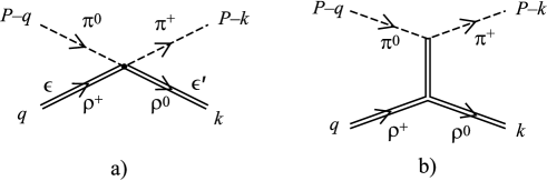
Figure 1: a) Contact interaction from the Lagrangian of Eq. (20) for the $\rho^{+}\pi^{0}\to\rho^{0}\pi^{+}$; b) Corresponding diagram provided by the HGS formalism.

The HGS formalism leads to the diagram of Fig. 1b), which can be readily evaluated and approximated using the Feynman rules of the Appendix.

$${\cal L}^{HGS}_{\rho^{+}\pi^{0}\to\rho^{0}\pi^{+}}\simeq\frac{1}{2f^{2}}[(k+q)\cdot(2P-k-q)\epsilon\cdot\epsilon^{\prime}$$

$$-(2k-q)\cdot\epsilon~{}(2P-k-q)\cdot\epsilon^{\prime}-(2q-k)\cdot\epsilon^{\prime}~{}(2P-k-q)\cdot\epsilon],$$ (22)

where the intermediate $\rho$ propagator $[(q-k)^{2}-M_{V}^{2}]^{-1}$ has been approximated by $-M_{V}^{-2}$. As we can see, the first term of Eq. (22) coincides with the result of the chiral Lagrangian of Eq. (21). The second and third terms of Eq. (22) are small for small kinetic energies of the particles since the zeroth component of the polarization vectors tends to zero as the three-momentum of the vector meson goes to zero to satisfy the Lorenz condition $\epsilon\cdot q=0$. Under these conditions, the HGS formalism and the chiral Lagrangian of Eq. (20) provide the same vector-pseudoscalar meson interaction.

The kernel to be used in the Bethe-Salpeter equation is defined as

$$\widetilde{V}^{\prime}_{\rho^{+}\pi^{0}\to\rho^{0}\pi^{+}}\epsilon\cdot\epsilon^{\prime}=-{\cal L}_{\rho^{+}\pi^{0}\to\rho^{0}\pi^{+}}$$ (23)

which upon projection in isospin $I=1$, for the case of the $a_{1}^{+}$ resonance leads to

$$\widetilde{V}^{(I=1)}_{\rho\pi\to\rho\pi}\epsilon\cdot\epsilon^{\prime}=-\widetilde{V}^{\prime}_{\rho^{+}\pi^{0}\to\rho^{0}\pi^{+}}\epsilon\cdot\epsilon^{\prime}\simeq\frac{1}{2f^{2}}(k+q)\cdot(2P-k-q)\epsilon\cdot\epsilon^{\prime}$$ (24)

In Ref. [21] the spatial part $\vec{\epsilon}\cdot\vec{\epsilon}\,^{\prime}$ of the $I=1$ potential in s-wave was iterated in the Bethe-Salpeter equation, summing the diagrams of Fig. 2. The sum is done in Ref. [21] where the following scattering matrix is obtained:

$$T\simeq\frac{-\widetilde{V}}{1+\widetilde{V}G}\vec{\epsilon}\cdot\vec{\epsilon}\,^{\prime}$$ (25)

neglecting terms of $\rho$ momenta over the mass squared which are very small, where $G$ is the loop function of a $\rho$ and a $\pi$ conveniently regularized [21] corresponding to

$$G(P)=\int\frac{i\,d^{4}q}{(2\pi)^{4}}\frac{1}{q^{2}-m_{l}^{2}+i\epsilon}\frac{1}{(P-q)^{2}-M_{l}^{2}+i\epsilon}$$ (26)

The poles of the $T$-matrix, corresponding to the $a_{1}^{+}$ resonance require $1+\widetilde{V}G=0$ in the second Riemann sheet of the complex energy plane. In the real axis for the energy of the resonance we will have

$$\widetilde{V}G\sim-1\qquad\Longrightarrow\qquad G\sim-\widetilde{V}^{-1}.$$ (27)

This result is approximate because we go from the complex pole position to the real axis and also because in Ref. [21] the poles are searched solving the Bethe-Salpeter equations in coupled channels. However, since the coupling of $a_{1}^{+}$ to $\rho\pi$ is by far the largest [21], the result of Eq. (27) is a rough approximation which will be used later on only for illustrative purposes.

Figure 2: Diagrammatic series of the Bethe-Salpeter equation for the $\rho\pi$ interaction.

4 Test of gauge invariance

Amplitudes which involve a photon must be computed in a way consistent with the gauge invariance. As a matter of fact, if all necessary diagrams are properly taken into account the gauge symmetry is satisfied. In some cases, however, its proof is not a trivial matter, especially when higher order loops are included or approximations are used. This happens in the present calculation, and therefore, we would like to discuss it in some detail.

Let us start with a brief look at a simple process of physical decay, $\rho\to\pi\pi\gamma$. This will be used later on to prove the gauge invariance of the diagrams involved in the axial-vector meson radiative decay. By using the Feynman rules of the Appendix, it is immediate to prove the gauge invariance of the set of diagrams shown in Fig. 4, upon summing the three diagrams and substituting $\epsilon^{(\gamma)}\to k$. This will be used later on to prove the gauge invariance of the diagrams involved in the axial-vector meson radiative decay. Independently, the set of diagrams of Fig. 3 is also gauge invariant.

The test of gauge invariance of the two sets succeeds when all the external particles are on shell. More concretely, in diagram c) of Fig. 4 the intermediate $\rho$ propagator is

$$\frac{1}{(q-k)^{2}-M_{V}^{2}}=\frac{1}{q^{2}-M_{V}^{2}-2qk}\to\frac{1}{-2qk}$$ (28)

In diagram c) of Fig. 3 the same occurs with the intermediate pion propagator. We must keep this in mind since when the $\rho^{+}$ in Fig. 4c) or the initial $\pi^{+}$ in Fig. 3c) are put inside a loop, as will be the case in the radiative decay, some extra diagram will be demanded to fulfill gauge invariance.

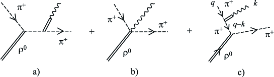
Figure 3: Set of Feynman diagrams which is gauge invariant for $\rho^{0}\to\pi^{+}\pi^{-}\gamma$.

Figure 4: Set of Feynman diagrams which is gauge invariant for $\rho^{+}\to\pi^{+}\pi^{0}\gamma$.

We shall continue considering the $\rho\pi$ channel, the most important of the $a_{1}$, for illustrative purposes, although in the final calculations we will consider the contribution of all the $VP$ coupled channels. Following Ref. [15] the radiative decay of the axial-vector mesons is obtained by coupling the photon to its meson components, which requires the knowledge of the coupling of the resonance to the different vector-pseudoscalar components. This coupling is of the type

$$V_{a_{1}^{+}\rho^{+}\pi^{0}}=g_{a_{1}^{+}\rho^{+}\pi^{0}}\epsilon_{A}\cdot\epsilon$$ (29)

with $\epsilon_{A}$, $\epsilon$, the polarization vectors of the axial and the vector mesons. The couplings $g_{i}$ are obtained in Ref. [21] from the residues at the pole positions of the scattering amplitudes. The set of diagrams needed for the calculation are given in Figs. 5 and 6

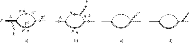
Figure 5: Gauge invariant set of diagrams for the radiative decay of the axial-vector meson.

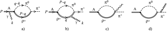
Figure 6: Another set of gauge invariant diagrams for the radiative decay of the axial-vector meson.

The connection of this formalism to details of the dynamical generation of the axial-vector mesons is discussed in Ref. [15] and in the analogous case of dynamically generated baryons in Ref. [35]. The gauge invariance of the set of diagrams in Figs. 3 and 4 would imply the gauge invariance of the set of diagrams b), c), d) in Figs. 5 and 6 if the $q$ lines were on the mass-shell. Since this is obviously not the case because they belong to a loop, the diagrams a) of Figs. 5 and 6 are demanded in order to still fulfill gauge invariance [14] because they cancel the effect of the off-shellness of the $q$ line in diagrams 5b) and 6b).

Indeed the pion propagator with momentum $q-k$ in Fig. 5b is

$$\frac{1}{(q-k)^{2}-m_{\pi}^{2}}=\frac{1}{q^{2}-m_{\pi}^{2}-2kq}$$

$$=\frac{1}{-2kq}+\left(\frac{1}{q^{2}-m_{\pi}^{2}-2kq}-\frac{1}{-2kq}\right)$$

$$=\frac{1}{-2kq}+\frac{1}{2kq}\,\frac{q^{2}-m_{\pi}^{2}}{(q-k)^{2}-m_{\pi}^{2}}.$$ (30)

The first term in Eq. (30) corresponds to the propagator of Eq. (28) assuming $q^{2}=m_{\pi}^{2}$ (on shell pion) and guarantees the cancellation of the last three diagrams of Fig. 5. The remnant term in Eq. (30) kills the propagator with momentum $q$, leaving a loop with just two propagators with momentum $q-k$ (pion) and $P-q$ (vector), which has then the same topology as the diagram of Fig. 5a). It is direct to see that with the following coupling of the photon to the axial-vector with positive charge in Fig. 5a,

$$-it_{A^{+}A^{+}\gamma}=-ie(P+P-k)_{\mu}\epsilon^{(\gamma)\mu}\epsilon_{A}\cdot\epsilon_{A}^{\prime},$$ (31)

the cancellation of Fig. 5a with the off-shell part of Fig. 5b, taking the second term of the pion propagator of Eq. (30), is exact and one has a gauge invariant set of diagrams. A similar reasoning can be made to show the gauge invariance of the set of Fig. 6. The Lagrangian of Eq. (31) could be obtained via minimum coupling neglecting terms of the same order as those neglected to convert the $VP\to VP$ interaction of the HGS in the one from the effective Lagrangian in section 3. Its use is demanded for consistency with the vertex chosen for the $VP\to VP$ interaction.

5 The radiative decay of the $a_{1}^{+}$ in the hidden gauge formalism

Although the diagrams $a,d$, of Figs. 5 and 6 are needed for the gauge invariance test, they give null contribution to the radiative decay amplitude for different reasons,

• diagram $a$: because of the requirement that the longitudinal component of the axial-vector propagator does not develop a pole of the pseudoscalar, which demands that the loop of Figs. 5a, 6a, vanishes for the external pion on shell as is the case here [37, 15].

• diagram $d$: because of the Lorenz condition of the axial-vector meson $P\cdot\epsilon_{A}=0$ [14, 36].

Therefore, one can perform the computation of the remaining diagrams $b$ and $c$ explicitly, but it is more rewarding to use a well known procedure which makes use of the gauge invariance of the set and automatically accounts for large cancellations which occur between these diagrams. Following [15] we write for the amplitude $a_{1}\to\gamma\pi$

$$T=\epsilon_{A\mu}\epsilon_{\nu}^{(\gamma)}T^{\mu\nu}$$ (32)

where $T^{\mu\nu}$ can be written, by Lorentz covariance, as

$$T^{\mu\nu}=a\,g^{\mu\nu}+b\,P^{\mu}P^{\nu}+c\,P^{\mu}k^{\nu}+d\,k^{\mu}P^{\nu}+e\,k^{\mu}k^{\nu}$$ (33)

where the coefficients $a,\cdots,e$ are Lorentz scalar functions of $P$ and $k$. Note that, due to the Lorenz condition, ${\epsilon_{A}}_{\mu}P^{\mu}=0$, ${\epsilon}_{\nu}^{(\gamma)}k^{\nu}=0$, all the terms in Eq. (32) vanish except for the $a$ and $d$ terms. On the other hand, gauge invariance implies that $T^{\mu\nu}k_{\nu}=0$, from where one gets

$$a=-d\,P\cdot k.$$ (34)

This is obviously valid in any reference frame, however, in the axial-vector meson rest frame and taking the Coulomb gauge for the photon, only the $a$ term survives in Eq. (32) since $\vec{P}=0$ and $\epsilon^{0}=0$. This means that, in the end, we will only need the $a$ coefficient for the evaluation of the process. However, the $a$ coefficient can be evaluated from the $d$ term thanks to Eq. (34). The advantage of doing this is that there are few mechanisms contributing to the $d$ term and by dimensional reasons the number of powers of the loop momentum in the numerator will be reduced, as will be clearly manifest from the discussion below.

In the present case it is easy to see that the diagrams $c$ of Figs. 5 and 6 do not contribute to the $d$ coefficient and hence one only has to evaluate the diagrams $b$ of Figs. 5 and 6. The details on how to evaluate the $d$ coefficient using the Feynman parametrization of the amplitudes are given in Ref. [15]. The only difference from the previous case is in the diagram Fig. 6 b) where the effective $\gamma VV$ vertex mediated by the vector meson propagator through the vector meson dominance has extra terms (see section 7 for more details). It turns out that the presence of the extra terms which come from the self-interaction vertex of a non-abelian gauge theory plays a crucial role to make the $d$-coefficient extracted from Fig. 6 b) finite.

The total amplitude for the radiative decay is obtained as a sum over the diagrams of Figs. 5 and 6,

$$T=T^{Fig.\ref{fig:gaugeinvB1}}+T^{Fig.\ref{fig:gaugeinvB2}}\,.$$ (35)

For illustrative purposes we will consider in the present paper the same decays as in Ref. [15], which are $a_{1}^{+}\to\pi^{+}\gamma$ and $b_{1}^{+}\to\pi^{+}\gamma$. For these decays the $K^{*}K$ channels are also needed. The general expression for the amplitude for the kind of mechanisms shown in Figs. 5 and 6 are

$$T^{Fig.\ref{fig:gaugeinvB1}} = g^{\prime}_{AVP}Qc_{VPP}\frac{M_{V}G_{V}}{\sqrt{2}f^{2}}P\cdot k\,\epsilon_{A}\cdot\epsilon^{(\gamma)}$$ (36)

$$\times \int_{0}^{1}dx\int_{0}^{x}dy\frac{1}{8\pi^{2}}\frac{1}{s+i\varepsilon}\left((1-x)(2-y)-y(1-x)\frac{m_{\pi^{+}}^{2}-m_{P}^{2}}{M_{V}^{2}}\right),$$

where

$$s=(1-x)(xM_{A}^{2}-M_{V}^{2}-2yP\cdot k)-xm_{P}^{2},$$ (37)

with $m_{P}$ and $M_{V}$ the masses of the pseudoscalar and vector mesons in the loop, $m_{\pi^{+}}$ the mass of the final state pion and $M_{A}$ the mass of the axial vector meson,

$$T^{Fig.\ref{fig:gaugeinvB2}} = -g^{\prime}_{AVP}Qc_{VPP}\frac{M_{V}G_{V}}{\sqrt{2}f^{2}}P\cdot k\,\epsilon_{A}\cdot\epsilon^{(\gamma)}$$ (38)

$$\times \int_{0}^{1}dx\int_{0}^{x}dy\frac{1}{16\pi^{2}}\frac{1}{s^{\prime}+i\varepsilon}\left(5x-2y+xy-y(1-x)\frac{m_{\pi^{+}}^{2}-m_{P}^{2}}{M_{V}^{2}}\right),$$

where

$$s^{\prime}=(1-x)(xM_{A}^{2}-m_{P}^{2}-2yP\cdot k)-xM_{V}^{2}.$$ (39)

In Eqs. (36) and (38), $g^{\prime}_{AVP}$ are the $AVP$ coupling constants in the charge base. These coefficients are related to the $g_{AVP}$ in isospin base, obtained in Ref. [21], through the transformation

$$g^{\prime}_{AVP}={\cal C}\times g_{AVP},$$ (40)

where ${\cal C}$ are coefficients which depend on the different $AVP$ channels. We use the values of $g_{AVP}$ obtained in Refs. [21, 15] by evaluating the residua at the pole position of the different $VP\to VP$ scattering amplitudes. In the previous equations, ${\cal C}$, $Q$ and $c_{VPP}$ are coefficients given in tables 1 and 2.

$a_{1}^{+}(1260)\rightarrow\pi^{+}\gamma$		${\cal C}$	$Q$	$c_{VPP}$
type Fig.5	$\overline{K^{*}}^{0}K^{+}$	$1/\sqrt{2}$	$-e$	$1$
	$\rho^{0}\pi^{+}$	$1/\sqrt{2}$	$-e$	$-\sqrt{2}$
type Fig.6	${K^{*}}^{+}\overline{K^{0}}$	$-1/\sqrt{2}$	$-e$	$-1$
	$\rho^{+}\pi^{0}$	$-1/\sqrt{2}$	$-e$	$\sqrt{2}$

Table 1: Coefficients for $a_{1}^{+}(1260)\rightarrow\pi^{+}\gamma$ decay.

$b_{1}^{+}(1235)\rightarrow\pi^{+}\gamma$		${\cal C}$	$Q$	$c_{VPP}$
type Fig.5	$\overline{K^{*}}^{0}K^{+}$	$1/\sqrt{2}$	$-e$	$1$
type Fig.6	${K^{*}}^{+}\overline{K^{0}}$	$1/\sqrt{2}$	$-e$	$-1$

Table 2: Coefficients for $b_{1}^{+}(1235)\rightarrow\pi^{+}\gamma$ decay.

6 Comparison of the results with the tree level

One is now asked to address the contribution of the tree level diagram of Fig. 7. Using the Feynman rules of the Appendix, one finds

$$T^{tree}=g_{a_{1}\rho^{0}\pi^{+}}\frac{e}{\sqrt{2}g}\epsilon_{A}\cdot\epsilon^{(\gamma)}\qquad;\qquad g_{a_{1}\rho^{0}\pi^{+}}=-g_{a_{1}\rho^{+}\pi^{0}}$$ (41)

However, this term should not be added in the hidden gauge formalism since it would lead to doublecounting. Indeed, we are going to prove that this term is identical to the diagram of Fig. 6b and thus it has already been counted. This observation was rightly stated in Ref. [19] and it holds for the HGS formalism. It cannot be applied to the model used in Ref. [15] where the diagram of Fig. 6b is not introduced and instead a direct coupling of the photon to the vector meson arising from minimal coupling in the Proca equation was used. We shall come back to this point later on.

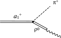
Figure 7: Tree level diagram for $a_{1}^{+}\to\gamma\pi^{+}$ decay.

Let us reinterpret the diagram of Fig. 6b in terms of the tree level diagram of Fig. 7. The essential argument comes by comparing the diagram of Fig. 6b with the diagrams for the dynamical generation of the $a_{1}$ as shown in Fig. 2. The relation to the former can be achieved by taking the limit $m_{V}\to$ large for the vector meson which emits the pion of the final state, as shown in Fig. 8. Since the heavy vector meson exchange has been used for the construction of $a_{1}$, the diagram of Fig. 8c, omitting the photon, is equivalent to the sum over diagrams of Fig. 2 excluding the first tree diagram. Near the resonance pole of $a_{1}$, however, the first tree diagram can be neglected and hence the diagram of Fig. 8c, omitting the photon, becomes equivalent to Fig. 2. This enables one to reinterpret the diagram of Fig. 6b (or 8d) as equivalent to the tree diagram of Fig. 7.

Let us see how this occurs analytically. For this purpose we factorize the vertex of $VP\to VP$ in terms of the potential $\widetilde{V}^{\prime}$ of Eq. (24). Then the diagram 6b now acquires the topology of Fig. 8d and can be computed as

$$-iT^{Fig.\ref{fig:Vp}d} = -ig_{a_{1}\rho^{+}\pi^{0}}\int\frac{d^{4}q}{(2\pi)^{4}}\,\epsilon_{A}\cdot\epsilon\,\frac{i}{q^{2}-m_{\pi}^{2}}\,\frac{i}{(P-q)^{2}-M_{V}^{2}}$$ (42)

$$\times (-i)\widetilde{V}^{\prime}_{\rho^{+}\pi^{0}\to\rho^{0}\pi^{+}}\,\epsilon\cdot\epsilon^{(\gamma)}\frac{i}{M_{V}^{2}}(-i)\frac{1}{\sqrt{2}}M_{V}^{2}\frac{e}{g}.$$

Summing over the $\epsilon$ polarization, neglecting the $q^{\mu}q^{\nu}/M_{V}^{2}$ terms of the $\rho$ propagator and considering Eq. (24) and the second of the eqs. (41), we have

$$T^{Fig.\ref{fig:Vp}d} \simeq -\,g_{a_{1}\rho^{+}\pi^{0}}\frac{e}{\sqrt{2}\,g}\widetilde{V}^{\prime}_{\rho^{+}\pi^{0}\to\rho^{0}\pi^{+}}G\,\epsilon_{A}\cdot\epsilon^{(\gamma)}$$ (43)

$$= -\,g_{a_{1}\rho^{0}\pi^{+}}\frac{e}{\sqrt{2}\,g}\widetilde{V}^{(I=1)}_{\rho\pi\to\rho\pi}G\,\epsilon_{A}\cdot\epsilon^{(\gamma)},$$

where $G$ is given by Eq. (26) and we regularize it as done in Ref. [21]. Eq. (43) coincides with Eq. (41) if $\widetilde{V}^{(I=1)}_{\rho\pi\to\rho\pi}G\simeq-1$, which is the condition at the pole position of the axial vector meson, as discussed in section 3. However, note that $\widetilde{V}^{(I=1)}_{\rho\pi\to\rho\pi}G\simeq-1$ is only true at the pole position and assuming one channel. Note also that in reality the $a_{1}$ resonance is very wide and hence it is far from the real axis, and also the effect of the other channels is not negligible. Furthermore, in the loop of Fig. 8d, the factorization of $\widetilde{V}^{(I=1)}_{\rho\pi\to\rho\pi}$ does not hold exactly (although quite accurately). Nevertheless, an actual exercise tells us that these two terms are of the same order of magnitude.

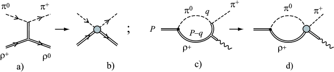
Figure 8: Vector meson exchange in the limit $m_{V}\to$ large.

The former discussion offers the possibility to evaluate the set of diagrams of Fig. 6 in a different way. We state that diagram 6b is the tree level of Fig. 7 and then we must add to it the diagram of Fig. 6c. This diagram is also evaluated with the same approximations done above and we obtain

$$T^{Fig.\ref{fig:gaugeinvB2}c}=g_{a_{1}\rho^{0}\pi^{+}}M_{V}^{2}\frac{e}{2\sqrt{2}\,gf^{2}}G\,\epsilon_{A}\cdot\epsilon^{(\gamma)}.$$ (44)

The ratio of $T^{Fig.\ref{fig:gaugeinvB2}c}$ to the tree level is estimated as

$$\frac{T^{Fig.\ref{fig:gaugeinvB2}c}}{T^{tree}}=G\frac{M_{V}^{2}}{2f^{2}}\simeq-\frac{M_{V}^{2}}{2f^{2}\widetilde{V}^{(I=1)}_{\rho\pi\to\rho\pi}}\simeq-\frac{M_{\rho}^{2}}{2M_{a_{1}}^{2}-2m_{\pi}^{2}-2M_{\rho}^{2}}\simeq-0.3.$$ (45)

This means that the whole set of diagrams of Fig. 6 can be approximated in terms of the tree level by

$$T^{Fig.\ref{fig:gaugeinvB2}}\simeq 0.7T^{tree}.$$ (46)

7 Comparison with a previous model

In this section we compare the results obtained in the hidden gauge formalism with those of the model of Ref. [15]. The model of Ref. [15] obtains the couplings via the Proca equation through minimal coupling. The diagrams obtained from the Proca equation corresponding to Fig. 5 are identical to those obtained in the previous sections. Those of Fig. 6 were the same except diagram 6b. This diagram was absent in the approach of Ref. [15]. Instead one had the diagram of Fig. 9a

Figure 9: a) and b): diagram and vertex used in the work of Ref. [15]; c): vertex used in the present work.

since minimal coupling on the Proca equation leads to a direct photon coupling to the vector meson, Fig. 9b. The diagram of Fig. 9b gives rise in this case to the contribution

$$T^{Fig.\ref{fig:diagold}b}=e[2\epsilon_{\alpha}^{(\gamma)}q^{\alpha}\epsilon^{\prime}_{\beta}\epsilon^{\beta}-\epsilon_{\alpha}^{(\gamma)}\epsilon^{\alpha}\epsilon^{\prime}_{\beta}q^{\beta}-\epsilon_{\alpha}^{(\gamma)}\epsilon^{\prime\alpha}\epsilon_{\beta}(q-k)^{\beta}],$$ (47)

while

$$T^{Fig.\ref{fig:diagold}c}=e[(2q-k)_{\alpha}\epsilon^{(\gamma)^{\alpha}}\epsilon_{\beta}\epsilon^{\prime\beta}-(q+k)^{\beta}\epsilon^{\prime}_{\beta}\epsilon_{\alpha}^{(\gamma)}\epsilon^{\alpha}+\epsilon_{\alpha}^{(\gamma)}\epsilon^{\prime\alpha}\epsilon_{\beta}(2k-q)^{\beta}].$$ (48)

Note that these two operators are different. As a consequence of this, the diagram of Fig. 9a cannot be identified with the tree level diagram.

It is worth looking at the difference between these two operators

$$T^{Fig.\ref{fig:diagold}c}-T^{Fig.\ref{fig:diagold}b}=e[k\cdot\epsilon\,\epsilon^{(\gamma)}\cdot\epsilon^{\prime}-k\cdot\epsilon^{\prime}\,\epsilon^{(\gamma)}\cdot\epsilon].$$ (49)

This difference is gauge invariant, which proves that if in the HGS approach the set of diagrams taken is gauge invariant, so was the set of diagrams taken in Ref. [15]. This was already stated there. Since, as we have shown, the diagram of Fig. 9a is not equivalent to the tree level, unlike the diagram of Fig. 6b, the question of the tree level diagram is reopen. Hence, in Ref. [15] the tree contribution was considered, invoking the approach of Refs. [29, 38] where it appears with strength similar to the one found here.

To continue with the comparison, let us quote further that the sum over the set of diagrams of Figs. 6a, 6c, 6d and 9a was found to provide a very small contribution, negligible in practice [15, 18]. As a consequence, for this set of diagrams plus the tree level one obtains essentially the tree level contribution, while the set of diagrams of Fig. 6 in the HGS formalism has been found to lead to a contribution about 0.7 times the tree level. The two formalisms hence lead to a difference of 30% of the tree level. Since the decay width is proportional to the square amplitude, its actual value in the HGS formalism is expected to be about a half ($0.7^{2}$) of the decay width from the tree amplitude. This rough estimation is indeed consistent with the present result as shown in tables 5 and 6.

8 New anomalous mechanisms

Besides those mechanisms considered so far, other diagrams could provide a relevant contribution to the radiative decay, like those shown in Fig. 10. The main peculiarity of the diagram of Fig. 10 is that it contains two anomalous $VVP$ vertices, which in principle one could expect to be small due to the higher order nature of the anomalous term in the chiral expansion. The $VVP$ interaction is anomalous[40] and accounts for a process that does not conserve intrinsic parity, and can be obtained from the gauged Wess-Zumino term (see e.g. Refs. [41, 42]). The expectation of small amplitudes was the reason why this double-anomalous mechanisms were not considered in Refs. [15, 18]. However, later works on the radiative decays of scalar mesons [30, 10] showed the importance of these mechanisms in radiative decay processes, which was also suggested in Ref. [13]. The importance of the anomalous process is also shown in another context of the kaon photoproduction [39]. In all these examples, as the relevant energy becomes larger the role of the anomalous contribution becomes more relevant. Therefore we are going to evaluate its contribution in the present work.

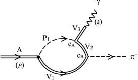
Figure 10: Feynman diagram containing the anomalous vertices.

The $VVP$ Lagrangian is [43, 44, 42]:

$${\cal L}_{VVP}=\frac{G^{\prime}}{\sqrt{2}}\epsilon^{\mu\nu\alpha\beta}\langle\partial_{\mu}V_{\mu}\partial_{\alpha}V_{\beta}P\rangle,$$ (50)

where $G^{\prime}=3g^{\prime 2}/(4\pi^{2}f)$ with $g^{\prime}=-G_{V}M_{\rho}/(\sqrt{2}f^{2})$. Since in the loops of Fig. 10 we have two vertices of the type $VVP$, the amplitude is proportional to $G^{\prime 2}$ or $g^{\prime 4}$. Hence, the contributions to the decay width of the loops of Fig. 10 go like $g^{\prime 8}$. Thus the decay width is very sensible to the exact value of the $VVP$ couplings. In order to fine tune the numerical value of the $VVP$ coupling we proceed in a similar way as in Ref. [30]: we normalize the $G^{\prime}$ coupling multiplying it by a factor $N_{i}$ such that the $V\to P\gamma$ decay widths agree with the experimental results (see Ref. [30] for details and exact definition of $N_{i}$).

The amplitude of the diagram of Fig. 10 is logarithmically divergent. Following the procedure of [30] one can isolate a divergent part having a loop structure with a pair of the same two meson propagators as appearing in the scattering problem (in the present case, a pseudoscalar and a vector). This term is naturally associated with the $VP$ loop function, $G_{VP}$, of Eq. (26). In Ref. [30], it was also shown that the logarithmically divergent term can be regularized with a cut off of natural size ($\sim 1$ GeV), having lead to very similar results. Thus we obtain:

$$T^{\rm anom} = g^{\prime}_{AP_{1}V_{1}}c_{A}c_{B}\lambda_{V_{3}}|e|\frac{N_{A}N_{B}G^{\prime 2}F_{V}}{2M_{V_{3}}}\epsilon_{A}\cdot\epsilon^{(\gamma)}P\cdot k$$

$$\times \left[\int_{0}^{1}dx\int_{0}^{x}dy\frac{1}{16\pi^{2}}\frac{1}{s+i\varepsilon}\left((P^{2}/2-k\cdot P)(1-x)^{2}-\frac{m_{V_{2}}^{2}}{2}\right)+\frac{1}{2}G_{VP}(P^{0},m_{V_{1}},m_{P_{1}})\right],$$

where $s=(P^{2}x-2P\cdot ky)(1-x)-m_{V_{1}}^{2}+(m_{V_{1}}^{2}-m_{P_{1}}^{2})x-(m_{V_{2}}^{2}-m_{P_{1}}^{2})y$ and $\lambda_{V}$ is $1$, $1/3$, $-\sqrt{2}/3$ for $V=\rho$, $\omega$, $\phi$ respectively. The coefficietns $c_{A}$ and $c_{B}$ are coming from the $VV^{\prime}P$ vertex defined as $c_{i}VV^{\prime}P$ after taking the trace in Eq. (50) and given in tables 3 and 4.

$a_{1}^{+}(1260)\rightarrow\pi^{+}\gamma$
$P_{1}V_{1}V_{2}V_{3}$	${\cal C}$	$c_{A}$	$c_{B}$
$\pi^{0}\rho^{+}\omega\rho^{0}$	$-1/\sqrt{2}$	$\sqrt{2}$	$\sqrt{2}$
$K^{+}\bar{K}^{*0}K^{*+}\rho^{0}$	$1/\sqrt{2}$	$1/\sqrt{2}$	1
$\bar{K}^{0}K^{*+}\bar{K}^{*0}\rho^{0}$	$-1/\sqrt{2}$	$-1/\sqrt{2}$	1

Table 3: Coefficients for the anomalous term of the $a_{1}^{+}(1260)\rightarrow\pi^{+}\gamma$ decay.

$b_{1}^{+}(1235)\rightarrow\pi^{+}\gamma$
$P_{1}V_{1}V_{2}V_{3}$	${\cal C}$	$c_{A}$	$c_{B}$
$\pi^{+}\omega\rho^{+}\omega$	$-1$	$\sqrt{2}$	$\sqrt{2}$
$\eta\rho^{+}\omega\omega$	$-1$	$2/\sqrt{3}$	$\sqrt{2}$
$K^{+}\bar{K}^{*0}K^{*+}\omega$	$1/\sqrt{2}$	$1/\sqrt{2}$	1
$K^{+}\bar{K}^{*0}K^{*+}\phi$	$1/\sqrt{2}$	1	1
$\bar{K}^{0}K^{*+}\bar{K}^{*0}\omega$	$1/\sqrt{2}$	$1/\sqrt{2}$	1
$\bar{K}^{0}K^{*+}\bar{K}^{*0}\phi$	$1/\sqrt{2}$	1	1

Table 4: Coefficients for the anomalous term of the $b_{1}^{+}(1235)\rightarrow\pi^{+}\gamma$ decay.

9 Numerical results

With the amplitudes obtained above, the decay width for the axial-vector mesons into one pseudoscalar meson and one photon is given by

$$\Gamma(M_{A})=\frac{|\vec{k}|}{12\pi M_{A}^{2}}|T|^{2},$$ (52)

where $M_{A}$ stands for the mass of the decaying axial-vector meson and $T$ is the sum of the amplitudes from the loop mechanisms removing the $\epsilon_{A}\cdot\epsilon$ factor. The former expression is valid for narrow axial-vector resonances. In order to take into account the finite width of the axial-vector meson we fold the previous expression with the mass distribution:

$$\Gamma_{A\rightarrow P\gamma}=-\frac{1}{\pi}\int_{(M_{A}-2\Gamma_{A})^{2}}^{(M_{A}+2\Gamma_{A})^{2}}ds_{A}\,Im\left\{\frac{1}{s_{A}-M_{A}^{2}+iM_{A}\Gamma_{A}}\right\}\Gamma(\sqrt{s_{A}})\Theta(\sqrt{s_{A}}-\sqrt{s_{A}^{th}}),$$ (53)

where $\Theta$ is the step function, $\Gamma_{A}$ is the total axial-vector meson width and $s_{A}^{th}$ is the threshold for the dominant $A$ decay channels.

Similarly, since the $\rho$ and $K^{*}$ mesons have relatively large widths, we have also taken into account the mass distribution of these states in the loop functions of Figs. 5 and 6. This is done by folding $T^{Fig.\ref{fig:gaugeinvB1}}$, $T^{Fig.\ref{fig:gaugeinvB2}}$, with the spectral function of the $\rho$ and $K^{*}$:

$$T^{Fig.\ref{fig:gaugeinvB1},Fig.\ref{fig:gaugeinvB2}}\to T^{Fig.\ref{fig:gaugeinvB1},Fig.\ref{fig:gaugeinvB2}}=-\frac{1}{\pi}\int_{(M_{V}-2\Gamma_{V})^{2}}^{(M_{V}+2\Gamma_{V})^{2}}ds_{V}\,Im\left\{\frac{1}{s_{V}-M_{V}^{2}+iM_{V}\Gamma_{V}}\right\}T^{Fig.\ref{fig:gaugeinvB1},Fig.\ref{fig:gaugeinvB2}}(\sqrt{s_{V}}).$$ (54)

The corrections from this source are small, they change the radiative decay widths at the level of $2$% or below.

In tables 5 and 6 we can see various contributions of different kinds of loops to the radiative decays. The theoretical errors have been obtained by doing a Monte-Carlo sampling of the parameters of the model within their uncertainties, as explained in Refs. [15, 18]. Due to the strong role played by the interferences between different mechanisms, as will be explained below, and the approximations involved in the relations between couplings, like those in Eq. (12), we have multiplied the errors by two to account safely for the theoretical uncertainties. We also show in the tables the result for the tree level with the model of Refs. [15, 18] which must not be consider if using the HGS formalism as explained in section 6. In the last row the experimental values provided by the PDG [23] are given, however these numbers refer to one single old experiment for each decay. From the table, the theoretical value of the total decay width for $a_{1}$ seems underestimated unlike the previous results [15], while for $b_{1}$ the agreement is good.

If we look at more details of the theoretical values, the amplitudes of Figs. 5 and 6 are destructively added for the $a_{1}$ decay, and the sum of them is smaller than each contribution. For the $b_{1}$ case this interference is constructive. In the present calculation, we have a new contribution from the anomalous term which is relatively large as compared to the normal contributions of Figs. 5 and 6 for the case of the $a_{1}$. It is also interesting to observe that the anomalous contribution is dominated by the $\rho\pi$ loop. It is therefore important to consider the anomalous terms if they exist. For the total theoretical amplitude for $a_{1}$ decay, the anomalous term has an opposite phase to the sum of contributions from Figs. 5 and 6, and so the net amplitude and the resulting decay width become small, 133 keV as compared with 640 $\pm$ 246 keV of the experimental value. For the case of $b_{1}$ the normal contributions already agree well as compared with experimental data, while the anomalous contribution is very small. Therefore, the total decay width agrees well with experimental data.

From the results in the tables it can be seen that the loops from Fig. 6 contribute much more than in the formalism of Refs. [15] where it was shown to be very small. This should not be surprising since the loop of Fig. 6b is very different from the one of Fig. 9a, evaluated in Ref. [15]. The actual value from the loop of Fig. 6 is consistent with the rough estimation of Eq. (46); for the case of $a_{1}$, they contribute 373 keV which is consistent with $0.7^{2}\times 647$ keV. For the case of the $b_{1}$ the argument holds only qualitatively; 57 keV of the contribution of Fig. 6 which is compared with the tree contribution of 67 keV.

$a_{1}^{+}(1260)\rightarrow\pi^{+}\gamma$
tree level with model of Refs. [15, 18]	$\phi$	-
	$\omega$	-
	$\rho$	647
	total	647
loops type Fig.5	$K^{*}K$	14
	$\rho\pi$	119
	total	171
loops type Fig.6	$K^{*}K$	30
	$\rho\pi$	213
	total	373
total (Fig.5+Fig.6)		103
loops anomalous	$\rho\pi$	163
	$\bar{K}^{*0}K^{+}$	1.4
	${K^{*}}^{+}\bar{K}^{0}$	1.4
	total	217
TOTAL (Fig.5+Fig.6+anomalous)		$133\pm 70$
experimental value [23]		$640\pm 246$

Table 5: Various contributions to the $a_{1}^{+}(1260)\rightarrow\pi^{+}\gamma$ decay width in units of keV.

$b_{1}^{+}(1235)\rightarrow\pi^{+}\gamma$
tree level with model of Refs. [15, 18]	$\phi$	20
	$\omega$	14
	$\rho$	-
	total	67
loops type Fig.5	$K^{*}K$	26
loops type Fig.6	$K^{*}K$	57
total (Fig.5+Fig.6)		159
loops anomalous	$\omega\pi$	2.2
	$\rho\eta$	0.6
	$\bar{K}^{*0}K^{+}(\omega)$	$6.3\times 10^{-2}$
	$\bar{K}^{*0}K^{+}(\phi)$	0.1
	${K^{*}}^{+}\bar{K}^{0}(\omega)$	$6.3\times 10^{-2}$
	${K^{*}}^{+}\bar{K}^{0}(\phi)$	0.1
	total	4
TOTAL (Fig.5+Fig.6+anomalous)		$209\pm 90$
experimental value [23]		$230\pm 60$

Table 6: Various contributions to the $b_{1}^{+}(1235)\rightarrow\pi^{+}\gamma$ decay width in units of keV.

10 Conclusions

We have developed the formalism to evaluate the radiative decay of axial vector mesons from the perspective that these states are composite particles of pseudoscalar and vector mesons, using the hidden gauge formalism for the interaction of vector mesons and pseudoscalars among themselves and with external sources. The formalism is rather rewarding. It shows a clear path to proceed and allows the interpretation of the tree level diagrams which in other formalisms are more difficult to integrate within the corresponding scheme. Also, one finds finite radiative decay widths which we compare with present experimental results considering theoretical and experimental uncertainties. We found good results for the radiative decay of the $b_{1}(1235)$ resonance, while not so good for the $a_{1}(1260)$ resonance, where large cancellations occurred in the theoretical framework. Because of these large cancellations of the main mechanism, extra corrections stemming from the consideration of loops involving anomalous couplings and extra vector mesons gave a non-negligible contribution to the radiative decay width. The improvement is, however, not remarkable. For the case of $b_{1}$ the agreement of the basic mechanism with data was already rather good, while the anomalous contributions played only a minor role.

The finite results obtained within the hidden gauge formalism and the simplicity of the approach make the use of this formalism practical and advisable in this kind of problems. Even with the results for the $a_{1}$ resonance, the agreement with the data can be considered fair from the perspective that differences for radiative decays between models, and hence with data, are typically of the order of one or two orders of magnitude [1].

At the same time we have described the formalism with sufficient detail to use many of the results for related problems, like the interaction of vector mesons with pseudoscalars, linking the results to existing chiral Lagrangians, the interaction of vector mesons with themselves, etc. These results should prove useful in future work dealing with the interaction of vector mesons, which so far has not received much attention, and were one might expect that equally interesting results as found in other areas are lying ahead.

Appendix

Vertices involving $\rho$, $\pi$ and real photons. ($\epsilon$, $\epsilon^{\prime}$, polarization vectors for $\rho$, $\epsilon^{(\gamma)}$ for the photon).

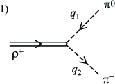
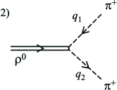
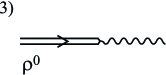
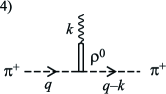
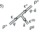
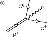
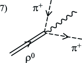
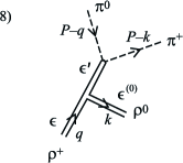
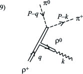
Figure 11:

$$-it^{Fig.\ref{fig:app1}}=-i\frac{M_{V}^{2}}{2\sqrt{2}gf^{2}}(q_{1}+q_{2})\cdot\epsilon,$$ (55)

$$-it^{Fig.\ref{fig:app2}}=i\frac{M_{V}^{2}}{2\sqrt{2}gf^{2}}(q_{1}+q_{2})\cdot\epsilon,$$ (56)

$$-it^{Fig.\ref{fig:app3}}=-ie\frac{M_{V}^{2}}{\sqrt{2}g}\epsilon\cdot\epsilon^{(\gamma)},$$ (57)

$$-it^{Fig.\ref{fig:app4}}=ie(q+q-k)\cdot\epsilon^{(\gamma)},$$ (58)

$$-it^{Fig.\ref{fig:app5}} = -i\sqrt{2}g[(k_{\mu}\epsilon^{(0)}_{\nu}-k_{\nu}\epsilon^{(0)}_{\mu})\epsilon^{\mu}\epsilon^{\prime\nu}$$ (59)

$$+ (-q_{\mu}\epsilon_{\nu}+q_{\nu}\epsilon_{\mu})\epsilon^{\prime\mu}\epsilon^{(0)\nu}+((q-k)_{\mu}\epsilon^{\prime}_{\nu}-(q-k)_{\nu}\epsilon^{\prime}_{\mu})\epsilon^{(0)\mu}\epsilon^{\nu}],$$

$$-it^{Fig.\ref{fig:app6}}=-ie\frac{M_{V}^{2}}{2\sqrt{2}gf^{2}}\epsilon\cdot\epsilon^{(\gamma)},$$ (60)

$$-it^{Fig.\ref{fig:app7}}=ie\frac{\sqrt{2}M_{V}^{2}}{2gf^{2}}\epsilon\cdot\epsilon^{(\gamma)},$$ (61)

$$-it^{Fig.\ref{fig:app8}} = -\frac{i}{2f^{2}}[(2k-q)\cdot\epsilon(2P-k-q)\cdot\epsilon^{(0)}$$ (62)

$$- (k+q)\cdot(2P-k-q)\epsilon\cdot\epsilon^{(0)}+(2q-k)\cdot\epsilon^{(0)}(2P-k-q)\cdot\epsilon],$$

(neglecting $(q-k)^{2}/M_{V}^{2}$)

$$-it^{Fig.\ref{fig:app9}} = -e\frac{i}{2\sqrt{2}gf^{2}}[(2k-q)\cdot\epsilon(2P-k-q)\cdot\epsilon^{(\gamma)}$$ (63)

$$- (k+q)\cdot(2P-k-q)\epsilon\cdot\epsilon^{(\gamma)}+(2q-k)\cdot\epsilon^{(\gamma)}(2P-k-q)\cdot\epsilon],$$

(neglecting $(q-k)^{2}/M_{V}^{2}$).

References

- [1] Yu. Kalashnikova, A. E. Kudryavtsev, A. V. Nefediev, J. Haidenbauer and C. Hanhart, Phys. Rev. C 73 (2006) 045203.
- [2] Z. G. Wang, Phys. Rev. D 75 (2007) 034013.
- [3] J. E. Palomar, L. Roca, E. Oset and M. J. Vicente Vacas, Nucl. Phys. A 729 (2003) 743.
- [4] V. E. Markushin, Eur. Phys. J. A 8 (2000) 389.
- [5] J. A. Oller, Nucl. Phys. A 727 (2003) 353.
- [6] J. A. Oller and E. Oset, Nucl. Phys. A 629 (1998) 739.
- [7] R. Escribano, P. Masjuan and J. Nadal, arXiv:0806.3007 [hep-ph].
- [8] J. E. Palomar, S. Hirenzaki and E. Oset, Nucl. Phys. A 707 (2002) 161.
- [9] D. Black, M. Harada and J. Schechter, Phys. Rev. Lett. 88, 181603 (2002) [arXiv:hep-ph/0202069].
- [10] H. Nagahiro, L. Roca, E. Oset and B. S. Zou, Phys. Rev. D 78 (2008) 014012.
- [11] T. Branz, T. Gutsche and V. E. Lyubovitskij, arXiv:0808.0705 [hep-ph].
- [12] S. Godfrey, Phys. Lett. B 568, 254 (2003); P. Colangelo and F. De Fazio, Phys. Lett. B 570, 180 (2003); W. A. Bardeen, E. J. Eichten and C. T. Hill, Phys. Rev. D 68, 054024 (2003); Fayyazuddin and Riazuddin, Phys. Rev. D 69, 114008 (2004); S. Ishida, M. Ishida, T. Komada, T. Maeda, M. Oda, K. Yamada and I. Yamauchi, AIP Conf. Proc. 717, 716 (2004); Y. I. Azimov and K. Goeke, Eur. Phys. J. A 21, 501 (2004); P. Colangelo, F. De Fazio and A. Ozpineci, Phys. Rev. D 72, 074004 (2005); F. E. Close and E. S. Swanson, Phys. Rev. D 72, 094004 (2005); X. Liu, Y. M. Yu, S. M. Zhao and X. Q. Li, Eur. Phys. J. C 47, 445 (2006); Z. G. Wang, J. Phys. G 34, 753 (2007); D. Gamermann, L. R. Dai and E. Oset, Phys. Rev. C 76 (2007) 055205
- [13] M. F. M. Lutz and M. Soyeur, arXiv:0710.1545 [hep-ph].
- [14] A. Faessler, T. Gutsche, V. E. Lyubovitskij and Y. L. Ma, Phys. Rev. D 76, 014005 (2007).
- [15] L. Roca, A. Hosaka and E. Oset, Phys. Lett. B 658, 17 (2007).
- [16] Y. b. Dong, A. Faessler, T. Gutsche and V. E. Lyubovitskij, Phys. Rev. D 77, 094013 (2008) [arXiv:0802.3610 [hep-ph]].
- [17] A. Faessler, T. Gutsche, V. E. Lyubovitskij and Y. L. Ma, Phys. Rev. D 76, 114008 (2007) [arXiv:0709.3946 [hep-ph]].
- [18] H. Nagahiro, L. Roca and E. Oset, Phys. Rev. D 77, 034017 (2008).
- [19] M. F. M. Lutz and S. Leupold, arXiv:0801.3821 [nucl-th].
- [20] M. F. M. Lutz and E. E. Kolomeitsev, Nucl. Phys. A 730, 392 (2004).
- [21] L. Roca, E. Oset and J. Singh, Phys. Rev. D 72, 014002 (2005).
- [22] L. S. Geng, E. Oset, L. Roca and J. A. Oller, Phys. Rev. D 75 (2007) 014017.
- [23] C. Amsler et al. [Particle Data Group], Phys. Lett. B 667 (2008) 1.
- [24] E. Marco, S. Hirenzaki, E. Oset and H. Toki, Phys. Lett. B 470, 20 (1999) [arXiv:hep-ph/9903217].
- [25] M. Bando, T. Kugo, S. Uehara, K. Yamawaki and T. Yanagida, Phys. Rev. Lett. 54, 1215 (1985).
- [26] M. Bando, T. Kugo and K. Yamawaki, Phys. Rept. 164 (1988) 217.
- [27] J. Gasser and H. Leutwyler, Nucl. Phys. B 250 (1985) 465.
- [28] G. Ecker, J. Gasser, H. Leutwyler, A. Pich and E. de Rafael, Phys. Lett. B 223, 425 (1989).
- [29] G. Ecker, J. Gasser, A. Pich and E. de Rafael, Nucl. Phys. B 321, 311 (1989).
- [30] H. Nagahiro, L. Roca and E. Oset, Eur. Phys. J. A 36 (2008) 73.
- [31] S. Weinberg, Phys. Rev. 166, 1568 (1968).
- [32] J. Sakurai, Currents and mesons (University of Chicago Press, Chicago, Il, 1969).
- [33] M. C. Birse, Z. Phys. A 355, 231 (1996) [arXiv:hep-ph/9603251].
- [34] K. Kawarabayashi and M. Suzuki, Phys. Rev. Lett. 16 (1966) 255; Riazuddin and Fayyazuddin, Phys. Rev. 147 (1966) 1071.
- [35] M. Doring, E. Oset and S. Sarkar, Phys. Rev. C 74, 065204 (2006).
- [36] D. Gamermann, L. R. Dai and E. Oset, Phys. Rev. C 76, 055205 (2007).
- [37] A. E. Kaloshin, Phys. Atom. Nucl. 60, 1179 (1997) [Yad. Fiz. 60N7, 1306 (1997)].
- [38] L. Roca, J. E. Palomar and E. Oset, Phys. Rev. D 70, 094006 (2004).
- [39] S. Ozaki, H. Nagahiro and A. Hosaka, Phys. Lett. B 665, 178 (2008) [arXiv:0710.5581 [hep-ph]].
- [40] J. Wess and B. Zumino, Phys. Rev. 163 (1967) 1727; J. Wess and B. Zumino, Phys. Lett. B37 (1971) 95;E. Witten, Ann. Phys. NY 128 (1980) 363; E. Witten, Nucl. Phys. B223 (1983) 422.
- [41] U. G. Meissner, Phys. Rept. 161 (1988) 213.
- [42] E. Pallante and R. Petronzio, Nucl. Phys. B 396 (1993) 205.
- [43] A. Bramon, A. Grau and G. Pancheri, Phys. Lett. B 283 (1992) 416.
- [44] E. Oset, J. R. Pelaez and L. Roca, Phys. Rev. D 67 (2003) 073013.