A Minimalist Turbulent Boundary Layer Model
Abstract
We introduce an elementary model of a turbulent boundary layer over a flat surface, given as a vertical random distribution of spanwise Lamb-Oseen vortex configurations placed over a non-slip boundary condition line. We are able to reproduce several important features of realistic flows, such as the viscous and logarithmic boundary sublayers, and the general behavior of the first statistical moments (turbulent intensity, skewness and flatness) of the streamwise velocity fluctuations. As an application, we advance some heuristic considerations on the boundary layer underlying kinematics that could be associated with the phenomenon of drag reduction by polymers, finding a suggestive support from its experimental signatures.
pacs:
47.27.-i, 47.27.nb, 47.27.DeTurbulent boundary layers have been a central topic of interest in fluid dynamic research for long years bl100 ; schli . Nevertheless their obvious technological importance, a satisfactory description of the physical mechanisms which underlie the boundary velocity fluctuations remains elusive to date. As the result of intensive computational and experimental efforts carried out mainly along the last two decades, it is by now clear that the turbulent boundary layer is the stage for the production and the complex interaction of coherent structures rob , a fact that was formerly antecipated by Theodorsen theo and Townsend town .
Standard phenomenological formulations of the turbulent boundary layer problem aim at solving self-consistent equations for the expectation values of velocity and the Reynolds stress tensor components, relevant quantities in engineering applications schli ; pope . At the very conception of these models no fundamental role is given to the whole boundary layer zoo of coherent structures, like streamwise and hairpin vortices, low speed streaks, etc. It is an open question, for instance, if a structural derivation of the Prandtl von-Karman logarithmic law of the wall is viable. In this sense, turbulent boundary layer modelling is a difficult problem of statistical physics, analogous to the derivation of thermodynamic equations of state from molecular kinematics/dynamics. The literature on the subject is still relatively small, although an initial discussion may be traced back to 1982 with Perry and Chong perry-chong .
This work differs from previous attempts perry-chong ; perry2 ; sree ; perry3 ; marusic1 ; marusic2 essentially in its stronger simplifying assumptions, specific coherent structure modelling (the vortex-dipole model to be introduced below), and the analysis of higher order statistics for the streamwise velocity fluctuations. We do not seek, at the present level of mathematical treatment, quantitative agreement with experiments; instead, we compute a set of general profiles, which turn out to be clearly supported by observations.
Our focus is on the streamwise fluctuations of the velocity field. Let us assume that close enough to the wall these fluctuations are mostly due to the flow generated by hairpin vortices head ; wu ; adrian , like the one depicted in Fig.1, momentarily located in the surroundings of the measurement position. The main contribution to streamwise fluctuations would come from the spanwise sector of hairpin vortices (also called “hairpin’s head” ), while subdominant contributions would be related to their necks and legs.

Since streamwise fluctuations of velocity are the only ones we have in mind, it is natural to replace the hairpin vortex by a simpler and more mathematically tractable structure, which we take to be a spanwise Lamb-Oseen vortex, an exact and non-stationary solution of the Navier-Stokes equations, described in cilindrical coordinates as
| (1) |
where is the total circulation around the vortex and is the squared vortex core radius at time , defined in terms of the kinematical viscosity .
Of course, (1) solves the fluid equations of motion in the absence of boundaries, so (1) is just a rough approximation to a real vortex parallel to the wall. In our modelling definitions, we postulate that the symmetry axis of the vortex lies in the plane (henceforth designed the “measurement plane”) that contains the measurement point and is normal to the wall. We assume, then, that at equally spaced time intervals, a given vortex is replaced by another one, at a random distance from the wall, with some prescribed probability distribution function (pdf) .

As the model under consideration is effectively two-dimensional, a mirror vortex is introduced “below the wall”, so that streamlines do not cross the material surface. Furthermore, in order not to completely neglect the non-slip boundary condition, some improvement is attained if we make the velocity field to vanish at the intersection of the measurement plane with the wall. For this purpose, an external homogeneous velocity field is superimposed to the field generated by the vortex dipole. These definitions are shown in Fig. 2.
An interpretation of the time dependence in Eq. (1) is in order. The time variable is taken to be the total time elapsed since the hairpin vortex was created at the wall. This assumption, however, is not of great help, if there is no way to relate the vortex vertical position to the time . To solve this problem, at least in a phenomenological fashion, we find inspiration in the scaling structure of the laminar boundary layer over a flat surface. It is well-established, and analytically predicted by the Blasius solution, that the laminar boundary layer thickness grows with the distance from the leading edge as . This result can be understood in elementary terms as the fact that any small perturbation which is transported along the main direction of the flow (say, the horizontal one) follows a diffusive drift along the vertical direction. An analogy to the context of turbulent boundary layers can be drawn, replacing words like “perturbations” by “coherent structures” and “molecular viscosity” by “eddy viscosity”. Actually, hairpin vortices are observed to grow in size as they get farther from the surface adrian . Therefore, we suppose that at time , a diffusion-like relation holds, and the vortex core radius can be written as in (1), where plays the role of a phenomenological parameter in the turbulent boundary layer modelling comment .
The flow depicted in Fig. 2 is assumed to describe a boundary layer with no pressure gradient. This is so because the velocity field is symmetric under reflections on the measurement plane. Pressure gradients are probably related to the flow induced by the whole gas of hairpin’s vortices, appearing, therefore, as a “many-body” effect.
We are now ready to work out a few relevant equations. Suppose that the Lamb-Oseen vortices are centered at and . The streamwise velocity field vanishes at point in Fig. 2. Once the resulting streamwise velocity is given as the sum of three contributions (the external, the real and the mirror vortex velocity fields), we get, using Eq. (1),
| (2) |
The above equation holds for any only if the total circulation is a dependent quantity. We find
| (3) |
It is a straightforward task to evaluate expectation values of general dependent functionals of the streamwise velocity field. It follows that
| (4) |
where the “two-point velocity”,
| (5) | |||||
is nothing but the velocity field at when the Lamb-Oseen vortices are placed at and .
We have applied (4) for a set of velocity functionals, comparing the dependent profiles so obtained with experimental results, as discussed below. As input parameters, we take , (i.e., the streamwise velocity is computed in units of the external velocity ). We use the pdf
| (6) |
with , to model fluctuations of the vortex’s height above the surface. It is important to note that the choice of the lorentzian distribution (6), although arbitrary, is by no means restrictive. We have checked out that smoothly decaying distributions lead to similar conclusions, if one is indeed interested in a qualitative understanding of turbulent boundary layer fluctuations.
The viscous and logarithmic layers
The mean streamwise velocity is obtained from the expectation value of . The overall profile is shown in Fig. 3, which interpolates between zero velocity at the wall and unit velocity at infinity. Even though seems to give a reasonable profile for the interval , the model does not apply to the outer layer, because of the stronger interactions between coherent structures and also for the high intermittency produced by the random entrainment of external laminar flow that take place in that region.

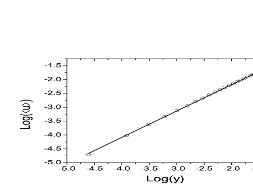
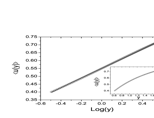
In Figs. 4 and 5, viscous and log-layers are clearly noticed for certain ranges of vertical distances. The excellent fit of the data to the straight line in Fig. 5 is given by . The numerical coefficients have precision of 0.1%. Observe that a purely dimensional argument yields in our particular model. Therefore, the numerical verification of a log-layer forces us to identify the effective external velocity to the friction velocity, up to numerical factors. We may conjecture, thus, that the friction velocity is “what is left” when a few dominant vortical structures near the wall are removed. In other words, the friction velocity can be interpreted here as a “mean field”, while fluctuations are modeled by isolated vortex dipoles.
Higher order statistics
Let . We introduce
| (7) |
and the hyperflatness functions , given by
| (8) |
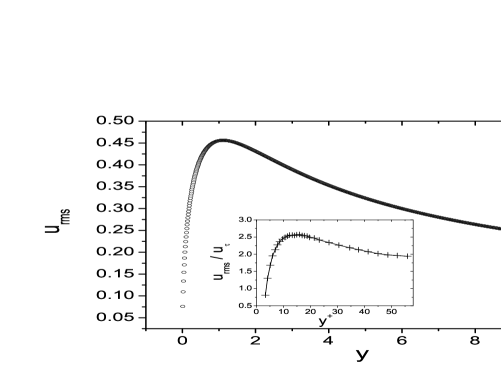
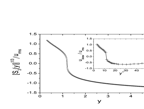
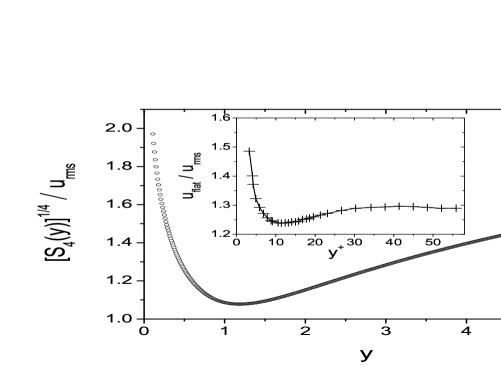
Fine measurements of turbulent boundary layer fluctuations for (skewness) and (flatness or kurtosis), which can resolve the region very close to the surface, are reported in Ref. lork . As we can see from Figs. 6, 7 and 8, there is a clear qualitative agreement with observations. In particular, the abrupt sign-changing transition of skewness is remarkably reproduced by the vortex dipole model.
Drag reduction by polymers
The phenomenon of drag reduction by polymers toms ; proc is a long-standing puzzle of non-newtonian fluid mechanics. The broad picture is that dissipation is attenuated due to the interaction of polymers with the coherent structures created near walls.
Recent PIV (particle image velocimetry) experiments in flows with dilute polymers have shown that vorticity fluctuations - and probably coherent structures - are supressed at some point above the surface in turbulent boundary layers white . Also, by about the same time, interesting signatures of drag reduction have been found in the profiles of and in connection with polymer dilution itoh . An additional peak is observed for , while the skewness shows further sign-changing transitions.
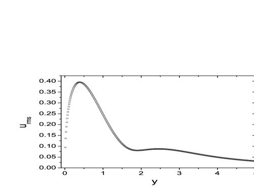
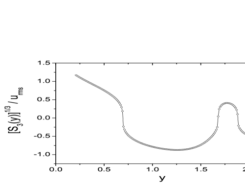
The vortex dipole model allows us to relate these apparently distinct features of drag reduction by polymers. Coherent structure supression can be naturally accounted for by changing the form of the vortex pdf . We take, for instance, a distribution which is uniform for , but vanishes for , that is,
| (9) |
where is the Heaviside function. Therefore, we suppose no vortex is found for , as the result of polymer interactions. Setting and keeping the previous definitions of , and , we get the results shown in Figs. 9 and 10, which are in striking correspondence with real profiles itoh .
We conclude with some general remarks. The present model does not take into account further aspects of the turbulent boundary layer phenomenology, which become important if the interest is shifted toward quantitative comparisons with experiments. An essential improvement, along the above lines, would be to introduce a pair of streamwise vortex configurations with opposite vorticity as a way to mimick hairpin legs. Only in this way it would be possible to compute the shear stress and, thus, define the physical scales of length and velocity which are necessary for the description of the inner boundary layer.
To summarize, we have introduced an elementary model of a turbulent boundary layer, focusing our attention on the streamwise fluctuations of velocity induced by hairpin vortices. The model’s main scope is to provide qualitative insights on the velocity and hyperflatness profiles. Up to the knowledge of the author, this is the first time the profiles of skewness and flatness of usual turbulent boundary layers, as well as certain statistical signatures of the phenomenon of drag reduction by polymers have been theoretically reproduced by means of vortex methods.
Acknowledgements.
This work has been partially supported by CNPq and FAPERJ. I thank Atila Freire for several interesting discussions and for calling my attention to Refs. perry-chong ; perry2 ; sree ; perry3 ; marusic1 . I also thank Katepalli Sreenivasan for kindly providing me a copy of Ref. sree .References
- (1) One Hundred Years of Boundary Layer Research, IUTAM Symposium, edited by G.E.A. Meier and K.R. Sreenivasan, Springer-Verlag (2004).
- (2) H. Schlicthing and K. Gersten, Boundary Layer Theory, Springer-Verlag, Berlin (2000).
- (3) S.K. Robinson, Annu. Rev. Fluid Mech. 23, 601 (1991).
- (4) T.Theodorsen, Mechanism of Turbulence in Proceedings of the Midwestern Conference on Fluid Mechanics, Ohio State University, Columbus, OH, (1952).
- (5) A.A. Townsend, The Structure of Turbulent Shear Flow, Cambridge University Press (1976).
- (6) S.B. Pope, Turbulent Flows, Cambridge University Press (2000).
- (7) A.E. Perry and M.S. Chong, J. Fluid Mech. 119, 173 (1982).
- (8) A.E. Perry, S.M. Henbest and M.S. Chong, J. Fluid Mech. 165, 163 (1986).
- (9) K.R. Sreenivasan, A Unified View of the Origin and Morphology of the Turbulent Boundary Layer Structure in Turbulence Management and Relaminarization, edited by H.W. Liepmann and R. Narasimha, Springer-Verlag (1987).
- (10) A.E. Perry and I. Marusic, J. Fluid Mech. 298, 361 (1995).
- (11) I. Marusic and A.E. Perry and , J. Fluid Mech. 298, 398 (1995).
- (12) I. Marusic, Phys. Fluids 13, 735 (2001).
- (13) M.R. Head and P. Bandyopadhyay, J. Fluid Mech. 107, 297 (1981).
- (14) Y. Wu and K.T. Christensenj, J. Fluid Mech. 568, 55 (2006).
- (15) R.J. Adrian, Phys. Fluids 19, 041301 (2007).
- (16) There is no strong argument to rule out a general anomalous diffusive ansatz, . We would not find, however, important qualitative departures for the results derived here.
- (17) T. Lorkowski, Small-Scale Forcing of a Turbulent Boundary Layer, FDRL TR 97-2, Fluid Dynamics Research Laboratory, Massachusetts Institute of Technology (1997).
- (18) B.A. Toms, in Proceedings of the International Congress on Rheology, p. 135, North-Holland, Amsterdam (1949).
- (19) I. Procaccia, V.S. L’Vov and R. Benzi, Rev. Mod. Phys. 80, 225 (2008).
- (20) C.M. White, V.S.R. Somandepalli and M.G. Mungal, Exp. Fluids 36, 62 (2004).
- (21) M. Itoh, S. Tamano, K. Yokota and M. Ninagawa, Phys. Fluids 17, 075107 (2005).