Proposition of the Interactive Pareto Iterated Local Search Procedure – Elements and Initial Experiments

Abstract

The article presents an approach to interactively solve multi-objective optimization problems. While the identification of efficient solutions is supported by computational intelligence techniques on the basis of local search, the search is directed by partial preference information obtained from the decision maker.

An application of the approach to biobjective portfolio optimization, modeled as the well-known knapsack problem, is reported, and experimental results are reported for benchmark instances taken from the literature. In brief, we obtain encouraging results that show the applicability of the approach to the described problem.

1 Introduction

As many problems of practical relevance are often characterized by several criteria that simultaneously have to be taken into consideration when solving the problem, multi-criteria approaches play an increasingly important role in many application areas of operations research, engineering, and computer science. Approaches from the domain of multi criteria decision making describe an alternative $x$, belonging to the set of feasible alternatives $X$, by a set of objective functions $Z(x)=\left(z_{1}(x),\ldots,z_{K}(x)\right)$. From a decision making perspective, these functions describe attributes of the alternatives, which are considered to be of relevance from the point of view of a decision maker, in a quantitative way. As the aspects and therefore the functions are however often of conflicting nature, not a single alternative exists being optimal for all $z_{k}(x)$. Instead, a set of equally Pareto-optimal alternatives can be found as introduced in the definitions below. Without loss of generality, we assume in the following Definitions 1.1 and 1.2 the maximization of the components $z_{k}(x)$ of $Z(x)$.

Definition 1.1 (Dominance)

A vector $Z(x)$ is said to dominate $Z(x^{\prime})$ iff $z_{k}(x)\geq z_{k}(x^{\prime})\forall k=1,\ldots,K\wedge\exists k\mid z_{k}(x)>z_{k}(x^{\prime})$. We denote the dominance of $Z(x)$ over $Z(x^{\prime})$ with $Z(x)\preceq Z(x^{\prime})$.

Definition 1.2 (Efficiency, Pareto-optimality)

The vector $Z(x),x\in X$ is said to be efficient iff $\not\!\exists Z(x^{\prime}),x^{\prime}\in X\mid Z(x^{\prime})\preceq Z(x)$. The corresponding alternative $x$ is called Pareto-optimal, the set of all Pareto-optimal alternatives Pareto-set $P$.

Two aspects play a vital role for solving multi-objective problems:

1. Search for optimal alternatives (the Pareto set $P$), supported by an optimization approach. In comparison to single-objective optimization approaches, the notion of optimality is here generalized with respect to the set of simultaneously considered optimality criteria.

2. Choice of a most-preferred solution by the decision maker of the particular situation. While in single-objective optimization problems, the choice of the most-preferred solution naturally follows the identification of the (single) optimal solution, in multi-objective problems an individual tradeoff between conflicting criteria has to be resolved in a decision making procedure.

Principally, three classes of combining search and decision making exist [1]:

1. A priori approaches reduce the multi-objective problem into a single-objective problem by constructing a utility function for the decision maker. The resolution of the problem then lies in the identification of the solution which maximizes the chosen utility function.

2. A posteriori approaches first identify the Pareto set $P$ (or a close and representative approximation) and then resolve the choice of a most-preferred solution within an interactive decision making procedure.

3. Interactive approaches combine search and decision making, presenting one or several solutions to the decision maker and collecting preference information which is then used to further guide the search for higher preferred alternatives.

The question, which particular way to follow when solving multi-objective optimization problems depends on several aspects. As mentioned above, a priori approaches require comparably rich preference information from the decision maker in order to reduce the problem to a single-objective problem. Assuming this information can be obtained, the resolution of the problem is straight-forward. Unfortunately, this is not necessarily the case in many situations as uncertainty about the precise appearance of the decision makers utility function is often present. Also, the acceptance of a single solution computed by a computational intelligence method may be a problematic issue from a psychological point of view for some decision makers as no further choice is possible.

A posteriori approaches on the other side do not require any information from a decision maker. Instead, the Pareto set $P$ is computed off-line, allowing the decision maker to perform other tasks while waiting for the results of the optimization procedure. Under the assumption that the set of optimality functions $Z(x)$ is exhaustive, an important aspect when formulating multi-objective models [2], one element $x^{*}\in P$ can be identified in a later decision making procedure as the most-preferred one. A potential drawback of this approach is however, that the Pareto-set may be of large cardinality, resulting in a necessary high computational effort when identifying the Pareto-optimal alternatives. Also, many if not most $x\in P$ are discarded in the decision making procedure as they do not meet the individual, personal requirements of the decision maker.

Interactive approaches may overcome the problems of the above described extreme ways of resolving multi-objective optimization problem. On one hand, only partial preference information is required when solving the problem as the search is guided in one direction which may be changed when obtaining less-preferred solutions. On the other hand, only fewer alternatives have to be computed compared to the entire Pareto-set $P$. An important aspect when implementing interactive approaches is, that the decision maker needs to be present during the resolution procedure. Also, the computation of the solutions has to be completed in little time as the decision maker will have to wait for the results of the system. With the increasing computational possibilities of modern, affordable computer systems, the proposition and implementation interactive approaches however becomes more and more attractive.

Recent approaches of computational intelligence techniques implement interactive problem resolution procedures, e. g. on the basis of Evolutionary Algorithms [3], involving a decision maker during search. While in these approaches the set of criteria remains fixed during search, other concepts also include the possibility of dynamically changing the relevant criteria when searching for a most-preferred solution [4]. Research in interactive computational techniques is however a rather new field, and the precise way of how to integrate articulated preferences in the search process is still to be investigated in more detail.

In this article, we aim to contribute to the development of interactive computational intelligence techniques for the resolution of multi-objective optimization problems. While the search for Pareto-optimal alternatives is done by metaheuristics on the basis of local search, individual preferences guide the search in a particular direction with the goal of identifying a subset of $P$ that is considered to be of interest to the decision maker. While the idea is generic, it is tested on a particular application.

The article is organized as follows. In the following Section 2, the biobjective portfolio optimization problem is introduced and a quantitative optimization model is presented. We also briefly review existing approaches from the literature that have been used to solve this problem. An interactive procedure to solve the problem is proposed in Section 3. Experimental investigations on benchmark instances taken from literature follow in Section 4, and conclusions are drawn in Section 5.

2 Problem description

The multi-objective portfolio optimization problem consists in selecting a subset of assets from a set of $n$ possible investment possibilities such that several criteria, mainly the profit and risk of the resulting portfolio, are optimized. More formally, the following program has to be solved.

$$\max z_{k}(x)=\sum_{j=1}^{n}p_{j}^{k}\mathrm{x}_{j}\quad\forall k=1,\ldots,K$$ (1)

s. t.

$$\sum_{j=1}^{n}c_{j}\mathrm{x}_{j}\leq C$$ (2)

$$\mathrm{x}_{j}\in\{0,1\}$$ (3)

Each alternative $x$ consists of an $n$-dimensional decision vector $x=(\mathrm{x}_{1},\ldots,\mathrm{x}_{n})$ which defines for each asset $j$ whether it is included in the portfolio ($\mathrm{x}_{j}=1$) or not ($\mathrm{x}_{j}=0$), given in constraint (3). Side constraint (2) ensures that a given capacity (e. g. a budget) of $C$ is not exceeded, and typically the nonnegative coefficients $c_{j}$ relate to each other as $c_{j}\leq C\,\,\forall j=1,\ldots,n$ and $\sum_{j=1}^{n}c_{j}>C$. The nonnegative coefficients $p_{j}^{k}$ express for each $\mathrm{x}_{j}$ the contribution (e. g. the profit) of asset $j$ to objective $k$.

As the objectives conflict with each other, a set of Pareto-optimal alternatives $P$ exists among which the choice of a most-preferred solution $x^{*}\in P$ has to be made.

Unfortunately, the problem, also referred to as the so called knapsack problem, is $\mathcal{NP}$-hard [5], even for a $K=1$. For single-objective problems, relatively good branch-and-bound algorithms have been developed [6], other approaches are based on dynamic programming [7]. The multi-objective case with $K\geq 2$ has been tackled again with branch-and-bound [8] and several heuristics, mainly local search as e. g. Simulated Annealing [9], or Tabu Search [10].

3 Solution approach

Based on the discussion of different problem resolution strategies in Section 1 we propose an interactive metaheuristic that brings search and decision making together in a combined approach.

In the first step of the problem resolution approach, the decision maker is provided with lower and upper bounds of the particular problem. For the knapsack problem, this can be done by a set of weights $W$ and relaxing the binary constraint 3 for the computation of upper bounds. An example of a visual output is given in Figure 1, plotting the lower bound sets in blue, the upper bound sets in orange.

Figure 1: Lower/ upper approximation and determination of the goal vector

By means of the visualization of the lower and upper bounds, the decision maker may easily see the area in which Pareto-optimal solutions can be found. It becomes equally clear what values of $Z(x)$ are not possible as they would dominate an upper bound, enabling the decision maker to develop realistic expectations of a most-preferred solution $x^{*}$. In other words, objective values which are not achievable, as they lie outside the boundaries of the upper bounds, can be excluded from the decision making procedure.

The search for Pareto-optimal solutions is then guided by the articulation of a reference point $R=(r_{1},\ldots,r_{K})$, given in red color in Figure 1. This reference point defines a cone in outcome space which is used to specify an area in which the most-preferred solution $x^{*}$ is expected. After having successfully implemented an a posteriori strategy based on the same principle in which the identification of a most-preferred solution is supported by the progressive articulation of aspiration levels [11], we use this idea here to interactively guide the search.

Algorithm 1 Optimization framework

1:  Compute a first approximation $P^{approx}$ of $P$ using a set of weights $W$.

2:  Present $P^{approx}$ to the decision maker

3:  Obtain a reference point $R$ from the decision maker

4:  repeat

5:     Compute $P_{R}^{approx}$

6:     while $R$ has not been changed or termination criterion has not been met do

7:        Search for Pareto-optimal alternatives in the cone defined by $R$ by means of a pre-defined local search metaheuristic

8:        Constantly update $P_{R}^{approx}$ while searching for Pareto-optimal solutions

9:        Constantly update the visualization of $P_{R}^{approx}$, showing the results to the decision maker

10:     end while

11:  until termination criterion is met

The cone defined by $R$ is used to compute the set of alternatives $P_{R}^{approx}$ that dominate the reference point and therefore lie in the interior of the cone. In brief, $P_{R}^{approx}$ contains all elements $x\in P^{approx}\mid z_{k}(x)\geq r_{k}\forall k=1,\ldots,K$, therefore $P_{R}^{approx}\subseteq P^{approx}$. These alternatives are used by the Pareto Iterated Local Search metaheuristic, whose principle is sketched in Figure 2 and discussed in the following. Search continues until the decision maker terminates the process. This is going to be the case when a solution $x^{*}\in P_{R}^{approx}$ is found which meets the individual requirements and expectations of the decision maker as close as possible.

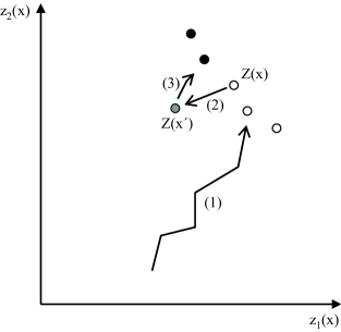
Figure 2: Pareto Iterated Local Search

Starting from an initial solution, a local search run is performed using a neighborhood operator until no further improvement is possible with simple local modifications. During this step, an archive of alternatives is maintained which contains all non-dominated alternatives found during search. While in the general procedure of Pareto Iterated Local Search [12] all non-dominated alternatives are kept, we here restrict the procedure to keep only alternatives in the cone defined by $R$ for further modifications/ improvements. In Figure 2, this stage of the procedure is visualized as step (1), with the results shown as white points in outcome space.

After having obtained a set of locally optimal alternatives, one of them is picked at random, see $Z(x)$ in Figure 2, perturbed into another alternative $x^{\prime}$ using some other neighborhood (2), and search is continued from here (3). As it can be seen in Figure 2, the perturbed solution may be dominated by one or several elements of $P_{R}^{approx}$, which has to be accepted when overcoming local optimality. In result, the metaheuristic iterates in interesting areas of the search space as opposed to restarting search from some other solution. This principle, known from Iterated Local Search [13], has been already successfully applied to other problems in which considerable fitness-distance-correlations have been found [14].

The computations of the metaheuristic are continued, constantly updating the plot of the Pareto-optimal alternatives in outcome space. During the problem resolution procedure, the decision maker is allowed modify the reference point, shifting the focus of the computations towards other regions. The problem resolution procedure terminates with the identification of a most-preferred solution $x^{*}$.

4 Experimental investigations

4.1 Experimental setup

The interactive Pareto Iterated Local Search has been tested on a benchmark instance taken from [10]. Apart from the fact that the optimal alternatives of these instances are known as mentioned above, the data sets are widely used for experimental investigations and comparison. In choosing them, we hope to provide a basis for fair and representative comparison. The data of the instance can be obtained from the internet homepage of the International Society on Multiple Criteria Decision Making under http://www.terry.uga.edu/mcdm/.

Local modifications of alternatives $x$ are done by randomly picking a single decision variable $\mathrm{x}_{j}\mid\mathrm{x}_{j}=1$, changing its value to $\mathrm{x}_{j}=0$, and randomly changing the value of other randomly chosen decision variables to 1 until no additional asset may be added to the solution.

We applied this local search neighborhood to each element in $P_{R}^{approx}$ until a dominating alternative has been found, replacing the alternative, or a subsequent number of 100 unsuccessful iterations has been tested on each element in $P_{R}^{approx}$. Then, the perturbation is applied to a randomly picked element in $P_{R}^{approx}$. The alternative is perturbed by changing two randomly chosen variables $\mathrm{x}_{j}=\mathrm{x}_{l}=1$ to 0 and refilling up the knapsack to the capacity $C$ by randomly selected other assets. In this sense, the perturbation is similar to the regular neighborhood, only that more decision variables are involved, leading to a bigger jump in the search space while keeping most of the characteristics of the perturbed alternative at the same time. The search then continues from the alternative which has been obtained through perturbation as described in Section 3.

In order to simulate the individual preference articulation of the decision maker, three reference points have been defined as given in table 1, one in the ‘knee-region’ [15] and two in the extreme areas of either one of the objective functions.

Table 1: Reference points

Model	Reference point	Vector
2KP50-50	ref. #1	$r_{1}=1807,r_{2}=1924$
2KP50-50	ref. #2	$r_{1}=2094,r_{2}=1800$
2KP50-50	ref. #3	$r_{1}=2166,r_{2}=1574$

100 test runs have been carried out with each reference point, keeping the approximations $P_{R}^{approx}$ for further analysis. In each test run 100,000 iterations have been allowed before terminating the search.

The quality of the computed approximations has been analyzed using the $M$ metric, given in expression 4. $M$ measures the percentage of identified Pareto-optimal alternatives in the cone defined by $R$.

$$M=\frac{|P_{R}^{approx}\cap P_{R}|}{|P_{R}|}$$ (4)

4.2 Results

Based on the data gathered in the experiments, the arithmetic mean values of $M$ have been computed, depending number of evaluations of the metaheuristic. These average values, given in Figure 3, clearly show that the iPILS metaheuristic successfully identified the Pareto-optimal alternatives in the particular areas of the reference points. However, there does not turn out to be a consistent difference for the three chosen reference points within the same instance.

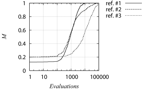
Figure 3: Results for 2KP50-50

While some approximations $P_{R}^{approx}$ already contain a Pareto-optimal alternative right from the start, no overall advantage for the final approximation quality results from this circumstance. Some areas are faster approximated, e. g. the one of reference point #1, others take considerable more time, see reference point #3.

5 Conclusions

The article presented an interactive method for the resolution of multi-objective optimization problems. The concept is based on the articulation of a reference point which expresses, from the point of view of the decision maker, an interesting area in outcome space. The computation of Pareto-optimal solutions is consequently focused on that region, identifying optimal solutions. In order to overcome locally optimal alternatives and converge to the front of the efficient solutions, a metaheuristic based on Iterated Local Search has been implemented.

Tests on the biobjective portfolio optimization problem have been carried out. In order to simulate a human decision maker, we assumed three different reference points for the investigated problem instance. Each one was chosen with respect to lower and upper bound sets that serve as an orientation for the decision maker. The problem resolution technique successfully solved the investigated benchmark instance, independent from the particular reference point.

Based on the investigations and experiments carried out, we conclude that the proposed concept may be a useful tool for solving multi-objective optimization problems, given the possibility to appropriately compute lower and upper bound sets of the particular problem. The results are encouraging, and deeper investigations on more instances will follow to support the results of the study.

References

- [1] J. Horn, “Multicriterion decision making,” in Handbook of Evolutionary Computation, T. Bäck, D. B. Fogel, and Z. Michalewicz, Eds. Bristol: Institute of Physics Publishing, 1997, ch. F1.9, pp. F1.9:1–F1.9:15.
- [2] D. Bouyssou, “Building criteria: A prerequisite for MCDA,” in Readings in Multiple Criteria Decision Aid, C. Bana E Costa, Ed. Heidelberg: Springer Verlag, 1990, pp. 58–80.
- [3] S. P. Phelps and M. Köksalan, “An interactive evolutionary metaheuristic for multiobjective combinatorial optimization,” Management Science, vol. 49, pp. 1726–1738, 2003.
- [4] M. J. Geiger and S. Petrovic, “An interactive multicriteria optimisation approach for scheduling,” in Artificial Intelligence Applications and Innovations, M. Bramer and V. Devedzic, Eds. Boston, Dordrecht, London: Kluwer Academic Publishers, 2004, pp. 475–484.
- [5] M. R. Garey and D. S. Johnson, Computers and Intractability—A Guide to the Theory of -Completeness. San Francisco, CA: W. H. Freeman and Company, 1979.
- [6] S. Martello and P. Toth, Knapsack Problems: Algorithms and Computer Implementations. Chichester, New York, Brisbane, Toronto, Singapore: John Wiley & Sons, 1990.
- [7] K. Klamroth and M. M. Wiecek, “Dynamic programming approaches to the multiple criteria knapsack problem,” Naval Research Logistics, vol. 47, pp. 57–76, 2000.
- [8] E. L. Ulungu and J. Teghem, “Solving multi-objective knapsack problem by a branch-and-bound procedure,” in Multicriteria Analysis, J. N. Climaco, Ed. Berlin, Heidelberg, New York: Springer Verlag, 1997, pp. 269–278.
- [9] E. L. Ulungu, J. Teghem, P. H. Fortemps, and D. Tuyttens, “MOSA method: A tool for solving multiobjective combinatorial optimization problems,” Journal of Multi-Criteria Decision Making, vol. 8, pp. 221–236, 1999.
- [10] X. Gandibleux and A. Freville, “Tabu search based procedure for solving the 0-1 multiobjective knapsack problem: the two objectives case,” Journal of Heuristics, vol. 6, no. 3, pp. 361–383, 2000.
- [11] M. J. Geiger, “Solving multi-objective scheduling problems—an integrated systems approach,” in Artificial Intelligence in Theory and Practice, ser. IFIP International Federation for Information Processing, M. Bramer, Ed. New York: Springer Verlag, 2006, vol. 217, pp. 493–502, ISBN 0-387-34654-6.
- [12] M. J. Geiger, “The PILS metaheuristic and its application to multi-objective machine scheduling,” in Multicriteria Decision Making and Fuzzy Systems – Theory, Methods and Applications, ser. Industrial and applied mathematics, K.-H. Küfer, H. Rommelfanger, C. Tammer, and K. Winkler, Eds. Aachen: Shaker Verlag, 2006, pp. 43–58, ISBN 3-8322-5540-0.
- [13] H. R. Lourenço, O. Martin, and T. Stützle, “Iterated local search,” in Handbook of Metaheuristics, ser. International Series in Operations Research & Management Science, F. Glover and G. A. Kochenberger, Eds. Boston, Dordrecht, London: Kluwer Academic Publishers, 2003, vol. 57, ch. 11, pp. 321–353.
- [14] K. D. Boese, “Models for iterative global optimization,” Ph.D. dissertation, University of California at Los Angeles, Los Angeles, California, 1996.
- [15] L. Rachmawati and D. Srinivas, “A multi-objective genetic algorithm with controllable convergence on knee regions,” in 2006 IEEE Congress on Evolutionary Computation, Sheraton Vancouver Wall Centre Hotel, Vancouver, BC, Kanada, Juli 2006, pp. 6807–6814, ISBN 0-7803-9489-5.