van der Waals dispersion power laws for cleavage, exfoliation and stretching in multi-scale, layered systems

Abstract

Layered and nanotubular systems that are metallic or graphitic are known to exhibit unusual dispersive van der Waals (vdW) power laws under some circumstances. In this paper we investigate the vdW power laws of bulk and finite layered systems and their interactions with other layered systems and atoms in the electromagnetically non-retarded case. The investigation reveals substantial difference between ‘cleavage’ and ‘exfoliation’ of graphite and metals where cleavage obeys a $C_{2}D^{-2}$ vdW power law while exfoliation obeys a $C_{3}\log(D/D_{0})D^{-3}$ law for graphitics and a $C_{5/2}D^{-5/2}$ law for layered metals. This leads to questions of relevance in the interpretation of experimental results for these systems which have previously assumed more trival differences. Furthermore we gather further insight into the effect of scale on the vdW power laws of systems that simultaneously exhibit macroscopic and nanoscopic dimensions. We show that, for metallic and graphitic layered systems, the known “unusual” power laws can be reduced to standard or near standard power laws when the effective scale of one or more dimension is changed. This allows better identification of the systems for which the commonly employed ‘sum of $C_{6}D^{-6}$’ type vdW methods might be valid such as layered bulk to layered bulk and layered bulk to atom.

Layered bulk systems such as graphite and boron nitride have their atoms confined to a series of spatially discrete planes with interplanar distances significantly greater than the intraplanar atomic separations eg. 3.34Å vs 1.41Å for graphite. They can exhibit unusual electronic behaviour due to the nanometer scale of the layer thickness and macroscopic scale of the other two dimensions. This scale variation means that great care must be taken in investigating subtle physical effects such as dispersion forces as previous examples demonstrate Dobson et al. (2006); White and Dobson (2008); Gould et al. (2008).

All separated electronic systems exhibit long-range attractive potentials arising from instantenous electron fluctuations correlating via the Coloumb potential. These long-range potentials (often called van der Waals dispersion potentials when electromagnetic retardation is ignored) are typically absent from the commonest ab initio calculations such as DFT in the LDA or GGA, or are approximated by pair-wise inter-atomic potentials of the form $C_{6}D^{-6}$ which are ‘summed over’ in some way (see eg. refs Hasegawa and Nishidate (2004); Girifalco and Hodak (2002); Rydberg et al. (2003); Dappe et al. (2006); Ortmann et al. (2006); Hasegawa et al. (2007); Rydberg et al. (2003)) to obtain a new effective power law of the form $C_{n}D^{-n}$. Here the exponent $n$ is an integer and depends only on the geometry of the system while $C_{n}$ depends on the individual atoms as well as the geometry.

As summarised in Dobson et al. (2006) the exponent of an asymptotic power law in metallic and graphitic systems can depend on both the geometry and the type of material, with metals, graphene and insulators all differing. For example, with two parallel, nano-thin layers of a metal, graphene and insulator, the power-law exponents are $5/2$, $3$ and $4$ respectively (where insulators do obey a ‘sum over $D^{-6}$’ rule). When the number of layers is infinite we will show that the power depends not only on the type of material, but also the way the layers are divided. This will be investigated through three types of division: equal separation of all layers (‘stretching’), division into two sub-bulks (‘cleavage’) and removal of one layer from the top of a bulk (‘exfoliation’). Furthermore the interaction of layered bulks with atoms will be studied.

In this paper we investigate metallic and graphitic systems under these different types of division (insulators have trivial ‘sum over atoms’ exponents and need no further investigation). Neither metals nor graphitic systems are guaranteed to obey ‘sum over layer’ power laws and special care must be taken to evaluate their long-range correlation effects. As with previous workDob ; Pitarke and Eguiluz (1998); Dobson and Wang (1999); Furche (2001); Fuchs and Gonze (2002); Miyake et al. (2002); Gould (2003); Jung et al. (2004); Marini et al. (2006); Gould et al. (2008) we make use of the Adiabatic-Connection Formula and Fluctuation Dissipation Theorem (ACFFDT) under the random-phase approximation (RPA) to calculate the leading power laws under these different methods of division. All results in this paper are for the electromagnetically non-retarded case which Sernelius and Björk (1998) show to be unimportant in the range of interest for similar systems.

Stretched graphitic systems (‘straphite’) have already been studied in Gould et al. (2008) where it was shown that the dispersion potential for an infinite number of graphene layers, each with inter-layer spacing $D$ follows a $C_{3}D^{-3}$ asymptotic power law at $T=0$K where $C_{3}=0.80{\text{eV}}\text{\AA}^{3}$. We may make use of the same basic approach employed for graphitic layered systems to calculate the dispersion for metallic layered systems (we believe that graphite-metal intercalates may be examples of this type of system). For brevity we define an intralayer Coloumb potential multiplied by a density-density response function

$${\mathcal{C}}(q,u)={\bar{\chi}}(q,u){\bar{w}}(q)$$ (1)

where $q$ is the wavenumber parallel to the plane, ${\bar{\chi}}(q,u)$ is the non-interacting electron density-density response in a layer and ${\bar{w}}(q)$ is the Coloumb potential. When the system is metallic this takes the form ${\mathcal{C}}(q,u)=-\omega_{\rm{p2D}}(q)^{2}/u^{2}$ for $q\to 0$ where $\omega_{\rm{p2D}}(q)=(\frac{n_{0}e^{2}q}{2\epsilon_{0}m_{e}})^{1/2}$, $n_{0}=N_{{e^{-}}\rm{layer}}/A_{\rm{layer}}$ is the 2D electron density of each layer and $m_{e}$ is the mass of an electron. We may thus utilise equations 4 and 7 of ref. [Gould et al., 2008] and change variables to $\theta=qD$ and $\eta=\sqrt{D}\omega_{\rm{p2D}}(q)^{-1}u$ to show that the difference in the correlation energy per layer from the infinitely separated case takes the form

$$U_{\text{vdW}}\sim\frac{1}{D^{5/2}}\int_{0}^{1}{\text{d}}\lambda\int_{0}^{\infty}\theta^{3/2}{\text{d}}\theta\int_{0}^{\infty}d\eta\mathcal{G}(\theta,\eta,\lambda)$$ (2)

demonstrating a $C_{5/2}D^{-5/2}$ dispersion power law for layered metals. Numerical evaluation gives $C_{5/2}=9.26\hbar(\frac{n_{0}e^{2}}{2\epsilon_{0}m_{e}})^{1/2}$. As with graphitic systems this power law (although not the constant prefactor) is universal to all multi-layered metallic systems with an infinite stack of isotropically stretched layers.

System	$C_{n}^{\rm{system}}/C_{n}^{\rm{bi}}$	Predicted	Error
Tri-graphene	1.3632	1.4167	3.6%
Stretched graphite	2.1157	2.4041	14%
Tri-metal	1.3496	1.4512	7.5%
Stretched metal	2.0628	2.6830	30%

Table 1: Comparison of the system to bi-layer ratio of the per-layer vdW coefficients for graphitic and metallic systems, for tri-layered and stretched systems. Column 3 is obtained by summing over the individual layers and takes the form $\frac{2}{3}(2+2^{-n})$ for tri/bi and $2\zeta(p)$ for stretched/bi.

Given the universality of the van der Waals exponent for isotropic stretching of a given material it is worth exploring the validity of a ‘sum over $C_{n}D^{-n}$’ rule for layered systems. In Table 1 we present the ratio of the $C_{n}$ coefficient for a tri-layered or stretched system to the bi-layered system for metals and straphite as well as a the ‘sum over $C_{n}$’ prediction for this ratio (here $n$ is $3$ for straphite and $5/2$ for metals). The prediction is somewhat sound for straphite with an overprediction of $14\%$ for straphite but is much less so for metals where it leads to a $30\%$ overprediction of the potential. This suggests that, even using a correct power law, rules which effectively sum the coefficients may prove troublesome.

‘Cleavage’ represents another means of division of a layered system. Here the system is split between a single pair of layers to form two new layered systems. We refer to the new systems as half-bulks as opposed to the original full bulk. For homogenous, infinite layered systems the two are mirror images of each other.

Separating a layered bulk into two smaller half-bulks is equivalent to keeping all but one layer at an inter-layer spacing $d$ while increasing the remaining one to $D\gg d$ as in Figure 1 (we ignore any relaxation of the layers or layer spacing at the newly created surfaces). Here we are interested in the total dispersion energy per unit area rather than that per layer per area as in the previous case.

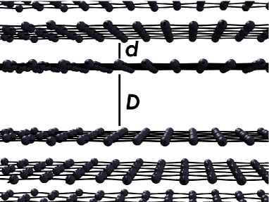
Figure 1: Layers after ‘cleavage’

We may make use of the second-order perturbation formula for the dispersion energy between the half-bulks while treating that within them to all orders (sometimes called the Zaremba-Kohn Zaremba and Kohn (1976) formula). Thus

$$U_{\text{vdW}}=\frac{-\hbar}{4\pi^{2}}\int_{0}^{\infty}{\text{d}}u\int_{0}^{\infty}q{\text{d}}q\mathcal{F}(q,u;D)$$ (3)

where

$$\mathcal{F}(q,u;D)\approx e^{-2qD}{{\text{Tr}}\left[({\mbox{\boldmath$\chi$}}_{\lambda=1}(q,u;d)\mbox{\boldmath$w$}^{b}(qD))^{2}\right]}$$ (4)

where $w^{b}_{ij}={\bar{w}}e^{-qd(i+j)}$ governs the interaction only between the two separate half-bulks while $\chi_{ij}$ is the full interacting response of the density in layer $i$ to a potential perturbation at layer $j$ within a single half-bulk.

Expanding the trace gives

$$\mathcal{F}=e^{-2qD}\sum_{ijkl}\chi_{ij}w^{b}_{jk}\chi_{kl}w^{b}_{li}=e^{-2qD}(\sum_{i}\delta n_{i}p^{i})^{2}$$ (5)

where $\delta n_{i}$ is the interacting electron density response of layer $i$ in the half-bulk to an external potential perturbation $\delta v_{i}={\bar{w}}p^{i}$ with $p=e^{-qd}$.

We may calculate $\delta n_{i}$ through the RPA equation $\delta n_{i}={\mathcal{C}}p^{i}+{\mathcal{C}}\sum_{j\geq 0}p^{|i-j|}\delta n_{j}$ where ${\mathcal{C}}={\mathcal{C}}(q,u)$ is as defined in equation (1). This gives the following recursion relationship

$$\delta n_{i+2}+\delta n_{i} =\left[(p+p^{-1})-{\mathcal{C}}(p-p^{-1})\right]\delta n_{i+1}$$ (6)

where $\delta n_{0}={\mathcal{C}}(1+\sum_{j\geq 0}p^{j}\delta n_{j})$ and we require $\delta n_{\infty}<\infty$. Writing a formal power series generating function $\mathcal{M}(x;{\mathcal{C}})=\sum_{i\geq 0}\delta n_{i}x^{i}$ transforms equation (6) into

$$(1+x^{2})\mathcal{M}(x;{\mathcal{C}})-\delta n_{0}-x\delta n_{1}=$$

$$\hskip 14.22636ptx\left[(p+p^{-1})+{\mathcal{C}}(p-p^{-1})\right](\mathcal{M}(x;{\mathcal{C}})-\delta n_{0})$$ (7)

so that (with correct series asymptotics)

$$\mathcal{M}(x;{\mathcal{C}}) =\frac{{\mathcal{C}}(p-p^{-1})}{p(1-r_{-}x)(1-r_{+}p^{-1})}$$ (8)

where $r_{\pm}=\zeta\pm\sqrt{\zeta^{2}-1}$, $\zeta=\frac{1}{2}(p+p^{-1})+\frac{1}{2}{\mathcal{C}}(p-p^{-1})$. Noting that $\sum_{i}p^{i}\delta n_{i}=\mathcal{M}(p)$ lets us write equation (5) as

$$\mathcal{F}(q,u;d,D)=e^{-2qD}\mathcal{M}(e^{-qd};{\mathcal{C}}(q,u))^{2}.$$ (9)

For graphite Dobson et al. (2006) shows that ${\mathcal{C}}(q,u)=\kappa[1+u^{2}/(v_{0}q)^{2}]^{-1/2}$ where $v_{0}=5.0\times 10^{5}\rm{ms}^{-1}$, $\kappa=\frac{e^{2}}{4\epsilon_{0}\hbar v_{0}}=12.1$. Defining $\alpha=d/D$, $\theta=qD$ and $\eta=ud/v_{0}$ lets us expand $\mathcal{F}(\theta,\eta)=\mathcal{F}(qD,ud/v_{0};\alpha,1)$ in powers of $\alpha$. To leading order this gives

$$\mathcal{F}(\theta,\eta)=e^{-2\theta}\frac{\kappa^{2}}{(\kappa+\eta+\sqrt{\eta^{2}+2\kappa\eta})^{2}}$$ (10)

for graphite. A similar change of variables yields a similar leading order expansion for metals. For these cases equation (3) gives a leading power law of exponent $n=2$ as with insulators.

Thus for grapite and metals we can write

$$U_{\text{vdW}}(D\to\infty)\approx\frac{C_{2}}{D^{2}}$$ (11)

where

$$C_{2}=\frac{-\hbar}{4\pi^{2}}\frac{\Gamma(2)}{2^{2}}\int_{0}^{\infty}{\text{d}}\eta T(\eta).$$ (12)

Here $T(\eta)=\frac{v_{0}}{d}\kappa^{2}(\kappa+\eta+\sqrt{\eta^{2}+2\kappa\eta})^{-2}$ for graphite and $T(\eta)=\frac{\omega_{\rm{p3D}}}{\sqrt{2}}(1+\eta^{2}+\eta\sqrt{\eta^{2}+2})^{-2}$ for metals with $\omega_{\rm{p3D}}=(\frac{n_{0}e^{2}}{\epsilon_{0}m_{e}d})^{1/2}$. For graphite we find $C_{2}=0.13d^{-1}{\text{eV}}\text{\AA}^{3}$ and for metals $C_{2}=1.6886\times 10^{-3}\hbar\omega_{\rm{p3D}}$. The latter result agrees exactly with continuous but anisotropic models of half-bulk metals where electron movement is restricted to be parallel to the surface, as is expected if the $d\to 0$ limit is well defined.

These results differ significantly from those expected by a simple sum-of-layers approach where we would expect graphene to obey a $C_{1}D^{-1}$ power law, and metals to obey a $C_{1/2}D^{-1/2}$ power law. The screening in these layered systems seems to cancel the different correlation effects of the individual layers so that they act as pseudo-insulating bulks.

Another means of dividing graphene (‘exfoliation’) is to peel a single layer of graphene from the top of a bulk. This represents yet another method of division where one system is a layered half-bulk and the other a single layer. We restrict our investigation to the case where the removed layer plane is always stiff and parallel to the planar surface of the bulk.

To model exfoliation we use a similar perturbative approach to cleavage but in equation (3) set $\mathcal{F}=e^{-2qD}\mathcal{M}(e^{-qd};{\mathcal{C}})\frac{{\mathcal{C}}}{1+{\mathcal{C}}}$ the product of the interacting response of a half-bulk and a single layer. For graphene this complicates the problem as the $\alpha=d/D\to 0$ limit works well for $\mathcal{M}$ but not for $\frac{{\mathcal{C}}}{1+{\mathcal{C}}}$. Here we keep $\alpha$ in the single-layer response only. Under transformation of variables $\theta=qD$ and $\eta=\frac{\alpha}{v_{0}}u$ (which already gives a $D^{-2}$ outside the integrals) we find

$$\mathcal{F}= \frac{v_{0}}{D}\kappa^{2}\theta e^{-2\theta}(\kappa+\eta+\sqrt{\eta^{2}+2\kappa\eta})^{-1}$$

$$\hskip 28.45274pt\times(\sqrt{\eta^{2}+(\alpha\theta)^{2}}+\kappa\alpha\theta)^{-1}.$$ (13)

Setting $\theta=1$ (where $\theta^{2}e^{-2\theta}$ takes its maximum), approximating $\sqrt{\eta^{2}+\alpha^{2}}$ by $\alpha+\eta$ and $\kappa+\eta+\sqrt{\eta^{2}+2\kappa\eta}$ by $2(\kappa+\eta)$ allows us to approximate the $\eta$ integral to show a leading $\alpha\log(\alpha)$ term. This is equivalent to a power law of the form

$$U_{\text{vdW}}(D\to\infty)\approx\frac{C_{3}\log(D/D_{0})}{D^{3}}.$$ (14)

and numerical calculation of equation (3) validates this assumption. For graphene (where $\kappa=12.1$) we find $D_{0}=0.16d$ and $C_{3}=0.07{\text{eV}}\text{\AA}^{3}$.

A similar analysis of metals shows a $C_{5/2}D^{-5/2}$ power law with $C_{5/2}=6.42\times 10^{-3}\sqrt{d}\hbar\omega_{\rm{p3D}}=9.07\times 10^{-3}\hbar\omega_{\rm{p2D}}(q=1)$. The $5/2$ power law is the same as that of a metal layer interacting with a continuum model of a metallic half-bulk as is, again, predicted by the limit of $d\to 0$.

While this analysis is not valid in the small $D$ regime it is worth noting that exfoliation and cleavage exhibit different power laws for graphite. This suggests that sum of $C_{6}$ models for converting experimental results from one to the other such as those employed in ref. [Benedict et al., 1998] may need reexamination. Unfortunately accurate calculation of the dispersion energy of such systems for $D\approx d_{0}$ (where $d_{0}$ is the layer spacing of graphite) is as yet intractable.

In nanoscale systems there are often combinations of molecules, layers and bulks. A simple example is an atom interacting with the surface of a layered metal or a molecule interacting with a graphene surface. Here the power law could be affected by the layering and electronic properties of the material.

In the coordinate system used for the layered models the interacting response function of an infinitely small “atom” located at $Z\hat{z}$ can be written as

$$\chi_{A}(\mathbf{q},\mathbf{q}^{\prime},z,{z^{\prime}};u)=$$

$$\hskip 14.22636pt\alpha(iu)\left[\mathbf{q}\cdot\mathbf{q}^{\prime}+\partial_{z}\partial_{{z^{\prime}}}\right]\delta(z-Z)\delta({z^{\prime}}-Z)$$ (15)

where $\mathbf{q}$ and $\mathbf{q}^{\prime}$ are reciprocal lattice vectors in the plane and $\alpha(iu)$ is the interacting dipole polarisibility of the atom at imaginary frequency $u$. This formula, used in equations (3-4), correctly reproduces the $C_{6}D^{-6}$ power law for interacting atoms.

We can use equation (15) to calculate the interaction of an atom with a layered bulk (metallic or graphitic) by making use of equations (3-4). This gives a power-law exponent $n=3$ in agreement with the prediction of a sum over $C_{6}D^{-6}$ potentials. This result strongly suggests that the unusual power laws exhibited by layered systems result from the interaction between long-range fluctuations in both systems and that removing them from one reduces the systems to ‘typical’ dispersive behaviour.

As has been seen here and in other workDobson et al. (2006); White and Dobson (2008); Gould et al. (2008) the asymptotic power law behaviour of layered systems can be anything but simple. Both graphitic and metallic systems exhibit vastly different dispersive power laws to insulators so that ‘sum of $C_{6}$’ approximations such as those typically employed cannot be used in the asymptotic region. It seems unlikely that, with such varied asymptotes, the cohesive energies and other similar measurables can be investigated using simple models.

	Graphite	Metal	Insulator
Stretching	$D^{-3}$	$D^{-5/2}$	$D^{-4}$
Cleavage	$D^{-2}$	$D^{-2}$	$D^{-2}$
Exfoliation	$\log(\frac{D}{D_{0}})D^{-3}$	$D^{-5/2}$	$D^{-3}$
Atom-bulk	$D^{-3}$	$D^{-3}$	$D^{-3}$

Table 2: Asymptotic power laws for various systems demonstrating both the material and structural dependence.

To illustrate these discrepancies we present in Table 2 a summary of the various power laws studied here. The insulator result represents the ‘classic’ sum over atomic power-laws behaviour of each system and any difference from its exponent represents ‘unusual’ behaviour.

While uniform stretching results in different power laws for metals, graphitics and insulators, cleavage removes this variation and involves the same exponent for all materials. This suggests that the interlayer screening induced by the Coulomb potential dominates the local response of each layer in the van der Waals energy for such systems converting their behaviour into that of non-layered or insulating bulks. This is further demonstrated by the fact that both the power law and coefficient of cleaved layered metals is the same as that of cleaved bulk metals with electron movement restricted to the plane.

By contrast, keeping a finite number of layers asymptotically isolated, as in exfoliation, or all layers asymptotically separated, as in stretching, returns different power-laws for different systems. In these cases at least one layer can be considered infinitesimally thin which we believe to be a requirement for the unusual power-laws. Replacing the isolated layer by an atom, however, returns the classical results which suggests that at least one large dimension is required for unusual vdW dispersion power-laws as postulated in refs. [Dobson et al., 2006; White and Dobson, 2008]

Overall, as this work and references Dobson et al. (2006); White and Dobson (2008); Gould et al. (2008) demonstrate, the dispersion forces of systems with a mix of nanometre and macroscopic length scales are more complex than classic Lifshitz theory predicts. As the differing power laws for cleavage and exfoliation demonstrate we must take great care in using indirectly derived cohesive energies from experiment.

These unusual van der Waals power laws may also have profound effects on the behaviour of many nanosystems. For certain systems it may be neccessary to adapt molecular dynamics and other semi-empirical and approximate ab initio simulation methods to account for these differences in order to best replicate experiment.

The authors acknowledge funding from the NHMA.

References

- Dobson et al. (2006) J. F. Dobson, A. White, and A. Rubio, Phys. Rev. Let. 96, 073201 (2006).
- White and Dobson (2008) A. White and J. F. Dobson, Phys. Rev. B 77, 075436 (2008).
- Gould et al. (2008) T. Gould, K. Simpkins, and J. F. Dobson, Phys. Rev. B 77, 165134 (2008).
- Hasegawa and Nishidate (2004) M. Hasegawa and K. Nishidate, Phys. Rev. B 70, 205431 (2004).
- Girifalco and Hodak (2002) L. A. Girifalco and M. Hodak, Phys. Rev. B 65, 125404 (2002).
- Rydberg et al. (2003) H. Rydberg, M. Dion, N. Jacobsen, E. Schröder, P. Hyldgaard, S. I. Simak, D. C. Langreth, and B. I. Lundqvist, Phys. Rev. Let. 91, 126402 (2003).
- Dappe et al. (2006) Y. J. Dappe, M. A. Basanta, F. Flores, and J. Ortega, Phys. Rev. B 74, 205434 (2006).
- Ortmann et al. (2006) F. Ortmann, F. Bechstedt, and W. G. Schmidt, Phys. Rev. B 73, 205101 (2006).
- Hasegawa et al. (2007) M. Hasegawa, K. Nishidate, and H. Iyetomi, Phys. Rev. B 76, 115424 (2007).
- (10) J. F. Dobson, in Topics in Condensed Matter Physics, edited by M. P. Das (Nova, New York, 1994), Chap. 7: see also cond-mat 0311371.
- Pitarke and Eguiluz (1998) J. M. Pitarke and A. G. Eguiluz, Phys. Rev. B 57, 6329 (1998).
- Dobson and Wang (1999) J. F. Dobson and J. Wang, Phys. Rev. Let. 82, 2123 (1999).
- Furche (2001) F. Furche, Phys. Rev. B 64, 195120 (2001).
- Fuchs and Gonze (2002) M. Fuchs and X. Gonze, Phys. Rev. B 65, 235109 (2002).
- Miyake et al. (2002) T. Miyake, F. Aryasetiawan, T. Kotani, M. van Schilfgaarde, M. Usuda, and K. Terakura, Phys. Rev. B 66, 245103 (2002).
- Gould (2003) T. Gould, Ph.D. thesis, Griffith University (2003), URL www4.gu.edu.au:8080/adt-root/public/adt-QGU20030818.125106/in%dex.html.
- Jung et al. (2004) J. Jung, P. García-González, J. F. Dobson, and R. W. Godby, Phys. Rev. B 70, 205107 (pages 11) (2004).
- Marini et al. (2006) A. Marini, P. García-González, and A. Rubio, Phys. Rev. Let. 96, 136404 (pages 4) (2006).
- Sernelius and Björk (1998) B. E. Sernelius and P. Björk, Phys. Rev. B 57, 6592 (1998).
- Zaremba and Kohn (1976) E. Zaremba and W. Kohn, Phys. Rev. B 13, 2270 (1976).
- Benedict et al. (1998) L. X. Benedict, N. G. Chopra, M. L. Cohen, A. Zettl, S. G. Louie, and V. H. Crespi, Chem. Phys. Letters 286, 490 (1998).