Compressive Wave Computation
Abstract
This paper considers large-scale simulations of wave propagation phenomena. We argue that it is possible to accurately compute a wavefield by decomposing it onto a largely incomplete set of eigenfunctions of the Helmholtz operator, chosen at random, and that this provides a natural way of parallelizing wave simulations for memory-intensive applications.
Where a standard eigenfunction expansion in general fails to be accurate if a single term is missing, a sparsity-promoting minimization problem can vastly enhance the quality of synthesis of a wavefield from low-dimensional spectral information. This phenomenon may be seen as ”compressive sampling in the Helmholtz domain”, and has recently been observed to have a bearing on the performance of data extrapolation techniques in seismic imaging [T. Lin and F. Herrmann, Geophysics, 2007].
This paper shows that -Helmholtz recovery also makes sense for wave computation, and identifies a regime in which it is provably effective: the one-dimensional wave equation with coefficients of small bounded variation. Under suitable assumptions we show that the number of eigenfunctions needed to evolve a sparse wavefield defined on points, accurately with very high probability, is bounded by
where is related to the desired accuracy and can be made to grow at a much slower rate than when the solution is sparse. The PDE estimates that underlie this result are new to the authors’ knowledge and may be of independent mathematical interest; they include an estimate for the wave equation, an estimate of extension of eigenfunctions, and a bound for eigenvalue gaps in Sturm-Liouville problems.
In practice, the compressive strategy makes sense because the computation of eigenfunctions can be assigned to different nodes of a cluster in an embarrassingly parallel way. Numerical examples are presented in one spatial dimension and show that as few as 10 percents of all eigenfunctions can suffice for accurate results. Availability of a good preconditioner for the Helmholtz equation is important and also discussed in the paper. Finally, we argue that the compressive viewpoint suggests a competitive parallel algorithm for an adjoint-state inversion method in reflection seismology.
Acknowledgements.
We would like to thank Ralph Smith and Jim Berger of the Statistical and Applied Mathematical Sciences Institute (SAMSI) for giving us the opportunity to visit the Institute, which catalyzed the completion of this project. We are indebted to Felix Herrmann for early discussions, Paul Rubin for help on a probability question related to Proposition 4, and Lexing Ying for help with a point in the numerical implementation of our preconditioner. Thanks are also due to Emmanuel Candès, Mark Embree, Jalal Fadili, Josselin Garnier, Mauro Maggioni, Justin Romberg, and William Symes for useful discussions. L.D. is supported in part by a grant from the National Science Foundation.
1 Introduction
In this paper we consider a simple model for acoustic waves,
| (1) |
with Dirichlet () or Neumann () boundary conditions. The parameter is viewed as the acoustic impedance of the medium, we will assume at least that , almost everywhere. In the sequel we will see how the classical equation of a vibrating string, with parameters and , can be transformed into (1) in such a way that all the results of this paper hold unaffected in the more general case.
Most numerical methods for solving (1) fall into two categories: either simulation in the time domain, by timestepping from initial and boundary data; or in the frequency domain using an expansion in terms of time-harmonic solutions. For the latter approach, when , then solves the Helmholtz equation
| (2) |
with Dirichlet or Neumann boundary conditions. The special values of for which (2) has a solution correspond to eigenvalues of the operator with the same boundary boundary conditions, through . The natural inner product that makes the operator self-adjoint is the one of the weighted space ,
| (3) |
(The regular inner product will not be used in the sequel.) Self-adjointness of classically implies orthogonality of the eigenfunctions, in the sense that . The operator is also negative definite (Dirichlet) or negative semi-definite (Neumann) with respect to the weighted inner product, which justifies the choice of sign for the eigenvalues. As a result, any solution of (1) can be expanded as
| (4) |
where
If we are ready to make assumptions on , however, equation (4) may not be the only way of synthesizing from its coefficients . The situation of interest in this paper is when is approximately sparse for each time , i.e, peaks at a few places in , and the impedance has minimal regularity properties. When these conditions are met, we shall see that the information of the solution is evenly spread, and contained several times over in the full collection of coefficients . In other words, there is a form of uncertainty principle to guarantee that a solution that peaks in cannot peak in , and that it is possible to decimate in such a way that a good approximation of can still be recovered. In addition, there exists a nonlinear procedure for this recovery task, which is so simple that it may have nontrivial implications for the numerical analysis of wave equations.
1.1 The Compressive Strategy
How to recover a sparse, sampled function from a set of discrete orthobasis coefficients , which is incomplete but nevertheless “contains the information” of , has been the concern of a vast body of recent work on compressed sensing [13, 28]. In this approach, the proposed solution for recovering is to find a vector with minimum norm among all vectors which have the observed as coefficients. Compressed sensing currently finds most of its applications in signal or image processing, but its philosophy turns out to be relevant for computational wave propagation as well, where the basis vectors are discretized eigenfunctions of the Helmholtz equation.
Accordingly, we formulate an problem for recovering at fixed time from a restricted set of coefficients . To guarantee that these coefficients be informative about , we will sample at random. For practical reasons explained later, we use the following sampling scheme: 1) draw a number uniformly at random between and some maximum value , 2) find the closest to , such that is an eigenvalue, 3) add this eigenvalue to a list provided it does not already belong to it, and 4) repeat until the size of the list reaches a preset value . Eventually, denote this list as .
Putting aside questions of discretization for the time being, the main steps of compressive wave computation are the following. Fix .
-
1.
Form the randomized set and compute the eigenvectors for ;
-
2.
Obtain the coefficients of the initial wavefields as and , for ;
-
3.
Form the coefficients of the solution at time as
-
4.
Solve the minimization problem
(5)
The algorithmic specifics of points 1 and 4 will be discussed at length in the sequel. The main result of this paper concerns the number of coefficients needed to ensure that the minimizer just introduced approximates within a controlled error, and controlled probability of failure.
1.2 Main Result
Specific notions of sparsity of the solution, and smoothness of the medium, will be used in the formulation of our main result.
-
•
Sparsity of the solution. Assume that is the solution of a discretization of the problem (1) on equispaced spatial points, i.e., . A central quantity in the analysis is the “size of the essential support” of this discretized solution, i.e., in a strategy that approximates by its largest entries in modulus, how large would need to be so that the error made is less than a threshold in a weighted sense. Then this particular choice of is called . More precisely, for fixed consider a tolerance , and the largest level at which
(6) where should be thought of as , or possibly a more sophisticated variant involving cell averages. Then is the number of terms in this sum, i.e., the number of grid points indexed by such that . In all cases , but the sparser the smaller .
-
•
Smoothness of the medium. We consider acoustic impedances with small total variation Var . In particular, we will require Var. See Section 3 for a discussion of total variation. Note that is permitted to have discontinuities in this model.
Three sources of error arise in the analysis: 1) the discretization error
where the norm is over ; 2) the truncation error just introduced, due to the lack of exact sparsity; and 3) a numerical error made in computing the discrete eigenvalues and eigenvectors, which shows as a discrepancy
for fixed , and where the norm is over . In addition to the absolute accuracy requirement that be small, we also need the following minor relative accuracy requirements for the eigenvalues and eigenvectors. Two quantities , are said to be within a factor 2 of each other if .
Definition 1.
(Faithful discretization) A spatial discretization of the Helmholtz equation (2) is called faithful if the following two properties are satisfied.
-
•
The gap between two consecutive eigenvalues of the discrete equation is within a factor 2 of the gap between the corresponding exact eigenvalues;
-
•
There exists a normalization of the computed eigenvectors and exact eigenvectors such that the discrete norm is within a factor 2 of , and simultaneously is within a factor 2 of .
Finally, we assume exact arithmetic throughout. The following theorem is our main result.
Theorem 1.
Assume that Var, and that the discretization of (2) is faithful in the sense of Definition 1. Assume that eigenvectors are drawn at random according to the procedure outlined above. There exists such that if obeys
| (7) |
(with sufficiently large so that all the logarithms are greater than 1), then with very high probability the solution of a discrete version of the minimization problem (5) obeys
| (8) |
Furthermore, can be taken to obey
| (9) |
where is a numerical constant. “Very high probability” here means where is an affine, increasing function of .
The discrete CWC algorithm is described in Section 2.2. The proof of Theorem 1 is in Sections 2.3 and 2.4.
Contrast this behavior of the problem by considering instead an regularization; by Plancherel the solution would then simply be the truncated sum
with error
This shows that may be very different from as soon as is not the complete set. In fact, the uncertainty principles discussed in this paper would show that the resulting error for sparse and random is large with very high probability.
The estimate (8) is a statement of robustness of the recovery method, and is intimately related to a well-established stability result in compressed sensing [12]. If errors are made in the discretization, in particular in computing eigenvectors on which the scheme is based , then equation (8) shows that this error will carry over to the result without being overly amplified. This robustness is particularly important in our context since in practice a compressive numerical scheme is bound to be the “driver” of a legacy code for the Helmholtz equation.
Theorem 1 also states that, if the discrete solution happens to be compactly supported on a small set ( for ), and no error is made in solving for the Helmholtz equation, then the compressive scheme would recover the discrete solution exactly, with high probability, and without using all the eigenvectors. It is not unreasonable to speak about compact support of the solution of a wave equation, since the speed of propagation is finite.
Another important point is that there exists no particular, “optimized” choice of the eigenvectors that can essentially beat choosing them at random. The compressive strategy, whether in numerical analysis or signal processing, is intrinsically probabilistic. In fact, making a deterministic choice can possibly void the reliability of recovery as there would exist counter-examples to Theorem 1.
Finally, the estimate is quite important from the viewpoint of computational complexity. In situations where is small, computing eigenvectors whose identity is unimportant as long as it is sufficiently randomized, can be much more advantageous than computing all of them. This leads to an easily parallelizable, frequency-based algorithm for the wave equation requiring at most operations instead of the usual for a QR method computing all eigenvectors. Complexity and parallelism questions are further discussed below.
1.3 Why It Works
The regularization is chosen on the basis that it promotes sparsity while at the same time defining a convex optimization problem amenable to fast algorithms. It provides an exact relaxation of problems when the vector to be recovered is sufficiently sparse, as was identified by David Donoho and co-workers in the mid-nineties in the scope of work on basis pursuit [18]. The same minimization extracts information of a sparse vector remarkably well in the presence of incomplete data, provided the data correspond to inner products in a basis like Fourier, for which there exists a form of uncertainty principle. This observation was probably first treated mathematically in 1989 in [29], and was refined using probabilistic techniques in work of Candès, Romberg, and Tao [13], as well as Donoho [28], both in 2004. This line of work received much attention and came to be known as compressed sensing or compressive sampling.
Consider the minimization problem in ,
where is a subset of , and is an orthobasis. The inner product is called a “measurement”. The following three conditions are prerequisites for guaranteeing the success of recovery of minimization.
-
1.
The vector to be recovered needs to be sparse;
-
2.
The basis vectors are incoherent; and
-
3.
The actual used as measurement vectors are chosen uniformly at random among the .
Sparsity of a vector can mean small support size, but in all realistic situations it is measured from the decay of its entries sorted in decreasing order. Typically, a vector is sparse when it has a small quasi-norm for , and the smaller the stronger the measure of sparsity.
Incoherence of an orthobasis of means that
| (10) |
where the parameter , simply called incoherence, is a reasonably small constant. For instance, if are the column of the isometric discrete Fourier transform, then attains its lower bound of , and the Fourier vectors are said to be maximally incoherent. The generalization where an orthobasis is incoherent with respect to another basis is often considered in the literature, in which case incoherence means small inner products of basis vectors from the two bases. Hence in our case we also speak of incoherence with respect to translated Diracs.
The condition of uniform random sampling of the measurement vectors is needed to avoid, with high probability, complications of an algebraic nature that may prevent injectivity of the projection of sparse vectors onto the restricted set of measurements, or at least deteriorate the related conditioning. More quantitatively, randomness allows to promote the incoherence condition into a so-called restricted isometry property (RIP). We will have more to say about this in the sequel. Note that if the measurement basis is itself generated randomly, e.g. as the columns of a random matrix with i.i.d. gaussian entries, then the further randomization of the measurement vectors is of course not necessary.
When these three conditions are met, the central question is the number of measurements needed for the recovery to succeed. Recent papers [14, 49] show that the best answer known to date is
where is the number of “big” entries in the vector to be recovered, is the incoherence, and is a decent constant. (The trailing log factors to the right of are conjectured to be unnecessary.) Stability estimates of the recovery accompany this result [12]. All this will be made precise in Section 2; let us only observe for now that (7) is manifestly a consequence of this body of theory.
The mathematical contribution of this paper is the verification that the conditions of 1) sparsity, 2) incoherence, and 3) uniform sampling are satisfied in presence of Helmholtz measurements for solutions of the wave equation, and in the context of a practical algorithm. For all three of these requirements, we will see that a single condition of bounded variation on suffices in one spatial dimension.
-
•
We show in Section 3.1 that when Var, the wave equation (1) obeys a Strichartz-like estimate
for , and where
This result shows that, in an sense, the sparser the initial conditions the sparser the solution at time . Hence choosing sparse initial conditions gives a control over the quality of recovery through the discrete quantity introduced above—although we don’t have a precise estimate to quantify this latter point.
-
•
We show in Section 3.2 that when Var, solutions of the Helmholtz equation must be extended, which translates into a property of incoherence at the discrete level. If solves (2), the extension estimate is
A quadrature of the integral on the right-hand side would reveal a factor , hence a comparison with the definition (10) of incoherence shows that the leading factor is in fact—modulo discretization questions—an upper bound on the incoherence of eigenfunctions with translated Diracs.
-
•
We show in Section 3.3 that when Var, two eigenvalues of the Helmholtz equation (2) cannot be too close to each other: if for are two distinct eigenvalues, then
This gap estimate shows that if we draw numbers uniformly at random within , and round them to the nearest for which is an eigenvalue, then the probabilities of selecting the -th eigenvalue are of comparable size uniformly in —again, modulo discretization questions. This provides control over departure from the uniform distribution, and quantifies the modest penalty incurred in the bound on as the ratio of probabilities
where refers to the case of uniform and equispaced .
Bounded variation can be thought of as the minimum smoothness requirement of an one-dimensional acoustic medium, for which wave propagation is somewhat coherent, and no localization occurs. For instance, the incoherence result physically says that the localization length is independent of the (temporal) frequency of the wave, for media of bounded variation.
1.4 How It Works
A classical algorithm for computing all eigenvectors of the discrete Helmholtz equation would be the QR method, with complexity an iterative . Since not all eigenvectors are required however, and since the discretized operator is an extremely sparse matrix, all-purpose linear algebra methods like QR acting on matrix elements one-by-one are at a big disadvantage.
Instead, it is more natural to set up a variant of the power method with randomized shifts for computing the desired eigenvectors and corresponding eigenvalues. We have chosen the restarted Arnoldi method coded in Matlab’s eigs command. In our context, the power method would compute the inverse for a shift chosen at random, and apply it repeatedly to a starting vector (with random i.i.d. entries, say), to see it converge to the eigenvector with eigenvalue closest to . The probability distribution to place on should match the spectral density of as closely as possible; one important piece of a priori information is the estimate (34) on eigenvalue gaps.
Applying , or in practice solving the system , can be done in complexity using an iterative method. However, the inversion needs not be very accurate at every step, and can be sped up using an adequate preconditioner. It is the subject of current research to bring the complexity of this step down to with a constant independent of frequency , see [34] for some of the latest developments. In this paper we use a particularly efficient preconditioner based on discrete symbol calculus [24] for pre-inverting (there is no typo in the sign), although the resulting overall complexity is still closer to than to .
The resolution of minimization can be done using standard convex optimization methods [8] such as interior point for linear programming in the noiseless setting, and second order cone programming in the noisy case [18]. One can however exploit the separability of the norm and design specific solvers such as exact [30] or approximate [32] path continuation and iterative thresholding [35, 22, 20, 54]. In this paper we used a simple iterative thresholding algorithm.
The complexity count is as follows:
-
•
It takes operations to solve for eigenvectors with a small constant, and as we have seen, is less than in situations of interest;
-
•
Forming spectral coefficients at time and their counterpart at time is obviously a operation.
-
•
It is known that solving an problem with degrees of freedom converges geometrically using the methods explained below [9] and is therefore a operation.
Compared to the QR method, or even to traditional timestepping methods for (1), the compressive scheme has a complexity that scales favorably with . The control that we have over the size of comes from the choice of sparse initial conditions, and also from the choice of time at which the solution is desired. If the initial conditions are not sparse enough, they can be partitioned into adequately narrow bumps by linearity; and if is too big, the interval can be divided into subintervals over which the compressive strategy can be repeated.
More details on the implementation can be found in Section 4.
1.5 Significance
The complexity count is favorable, but we believe the most important feature of the compressive solver, however, is that the computation of the eigenvectors is “embarrassingly parallel”, i.e., parallelizes without communication between the nodes of a computer cluster. This is unlike both traditional timestepping and Helmholtz-via-QR methods. The solver—proximal iterative thresholding—also parallelizes nicely and easily over the different eigenvectors, without setting up any domain decomposition method. We leave these “high-performance computing” aspects to a future communication.
Another decisive advantage of the compressive strategy is the ability to freely access the solution at different times. In inverse problems involving the wave equation, where an adjoint-state equation is used to form the gradient of a misfit functional, one is not just interested in solving the wave equation at a given time , but rather in forming combinations such as
where solves an initial-value problem, and solves a final-value problem—the adjoint-state wave equation. A classical timestepping method requires to keep large chunks of the history in memory, because is formed by time stepping up from , and is formed by time stepping down from . The resulting memory overhead in the scope of reverse-time migration in reflection seismology is well documented in [57]. The compressive scheme in principle alleviates these memory issues by minimizing the need for timestepping.
Let us also comment on the relief provided by the possibility of solving for incomplete sets of eigenvectors in the scope of compressive computing. As we saw, using an iterative power-type method has big advantages over a QR method. Could an iterative method with randomized shifts be used to compute all eigenvectors? The answer is hardly so, because we would need to “collect” all eigenvectors from repeated random sampling. This is the problem of coupon collecting in computer science; the number of realizations to obtain all coupons, or eigenvectors, with high probability, is with a rather large constant. If for instance we had already drawn all but one coupons, the expected number of draws for finding the last one is a —about as much as for drawing the first ones! For this reason, even if the required number of eigenvectors is a significant fraction of , the compressive strategy would remain attractive.
Finally, we are excited to see that considerations of compression in the eigenfunction domain requires new kinds of quantitative estimates concerning wave equations. We believe that the questions of sparsity, incoherence, and eigenvalue gaps are completely open in two spatial dimensions and higher, for coefficients that present interesting features like discontinuities.
1.6 Related Work
As mentioned in the abstract, and to the best of our knowledge, minimization using Helmholtz eigenfunctions as measurement basis vectors was first investigated in the context of seismic imaging by Lin and Herrmann [41] in 2007. Data extrapolation in seismology is typically done by marching the so-called single square root equation in depth; Herrmann and Lin show that each of those steps can be formulated as an optimization problem with an sparsity objective in a curvelet basis [11], and constraints involving incomplete sets of eigenfunctions of the horizontal Helmholtz operator. The depth-stepping problem has features that make it simpler than full wave propagation—extrapolation operators with small steps are pseudodifferential hence more prone to preserving sparsity than wave propagators—but [41] deals with many practical considerations that we have idealized away in this paper, such as the choice of basis, the higher dimensionality, and the handling of real-life data.
Sparsity alone, without using eigenfunctions or otherwise incoherent measurements, is also the basis for fast algorithms for the wave equation, particularly when the same equation needs to be solved several times. Special bases such as curvelets and wave atoms have been shown to provide sparse representations of wave propagators [51, 10]. Speedups of a factor as large as 20, over both spectral and finite difference methods, have been reported for a two-dimensional numerical method based on those ideas [25]. See also [33] for earlier work in one spatial dimension. Computational harmonic analysis for the solution of PDE has its roots in the concept of representing singular integral operators and solving elliptic problems using wavelets [44, 6, 19].
From a pure complexity viewpoint, methods based solely on decomposing the equation in a fixed basis are not entirely satisfactory however, because of the heavy tails of supposedly nearly-diagonal matrices. The resulting constants in the complexity estimates are cursed by the dimensionality of phase-space, as documented in [25]. There is also the question of flexibility vis-a-vis special domains or boundary conditions. We anticipate that representing the equation in an incoherent domain, instead, followed by a sparse recovery like in this paper may not suffer from the same ills.
Of course, sparsity and incoherence ideas have a long history in imaging problems unrelated to computation of PDE, including in geophysics [50]. As mentioned earlier, from the mathematical perspective this line of work has mostly emerged from the work of Donoho and collaborators [29, 18]. See [43] for a nice review.
Finally, previous mathematical work related to the theorems in Section 3 are discussed at the end of the respective proofs.
2 The Compressive Point of View: from Sampling to Computing
In this section we expand on the reasoning of Section 1.3 to justify Theorem 1. We first introduce the quoted recent results of sparse signal recovery.
2.1 Elements of Compressed Sensing
Consider for now the generic problem of recovering a sparse vector of from noisy measurements , with , and . The minimization problem of compressed sensing is
At this level of generality we call the measurement matrix and take its rows to be orthonormal. Accurate recovery of (P1) is only possible if the vectors are incoherent, i.e., if they are as different as possible from the basis in which is sparse, here Dirac deltas. Candès, Romberg and Tao make this precise by introducing the -restricted isometry constant , which is the smallest such that
| (11) |
for all subsets of such that , for all vectors supported on , and where is the sub-matrix extracted from by selecting the columns in . Equation (11) is called -restricted isometry property.
Candès, Romberg and Tao proved the following result in [12].
Theorem 2.
For , call the best approximation of with support size . Let be such that . Then the solution of (P1) obeys
| (12) |
The constants and depend only on the value of and .
Sparsity of is encoded in the rate of decay of as .
The problem of linking back the restricted isometry property to incoherence of rows was perhaps first considered by Candès and Tao in [14]. In this paper we will use the following refinement due to Rudelson and Vershynin [49]. It relates the allowable value of to the number of measurements and the dimension of the vector to be recovered.
Theorem 3.
Let be a -by- orthogonal matrix, and denote . Extract from by selecting rows uniformly at random. For every there exists a constant such that if
| (13) |
then obeys the -restricted isometry property (11) with and with very high probability.
Randomness plays a key role in this theorem; no instance of a corresponding deterministic result is currently known. Above, “very high probability” means tending to as , where is an affine increasing function of in (13). The proof of Theorem 3 in [49] uses arguments of geometric functional analysis and theory of probability in Banach spaces. Note that [49] prove the theorem for , but it is straightforward to keep track of the scaling by in their argument111For the interested reader, [49] denotes by . The scalings of some important quantities for the argument in [49], in their notations, are , , , and ..
2.2 Discretization
Equations (12) and (13) formally appear to be related to the claims made in Section 1.3, but we have yet to bridge the gap with the wave equation and its discretization.
Let us set up a consistent finite element discretization of (1) and (2), although it is clear that this choice is unessential. The Helmholtz equation with boundary conditions can be approximated as
where the stiffness matrix (a discretization of the second derivative) and the mass matrix properly include the boundary conditions. Square brackets indicate integer indices. Here is the discrete counterpart to the exact , and has multiplicity one, like , by the assumption of faithful discretization (Definition 1). The discrete eigenvector is an approximation of the eigenfunction samples .
We assume for convenience that the mass matrix can be lumped, and that we can write . If is smooth, then ; and if lacks the proper smoothness for mass lumping to be a reasonable operation, then all the results of this paper hold with minimal modifications. We also assume that is symmetric negative definite; as a result, so is , and the usual conclusions of spectral theory hold: , and are orthogonal for different , for the usual dot product in .
The corresponding semi-discrete wave equation (1) is
Because is the same stiffness matrix as above, the solution is
with
Call
A discretization error is incurred at time : we have already baptized it in the introduction. It is not the purpose of this paper to relate to the grid spacing. A nice reference for the construction of finite elements for the wave equation, in a setting far generalizing the smoothness assumptions made on in this paper, is in [47].
Let us now focus on the discrete formulation. The ideal problem that we would like to solve is
where are chosen uniformly at random.
In practice, we must however contend with the error in computing the discrete eigenvalues and eigenvectors by an iterative linear algebra method. This affects the value of as well as the measurement vectors in the equality constraints above. We model these errors by introducing the computed quantities and , and relaxing the problem to
| (14) |
for some adequate222Here is assumed to be known, but in practice it is permitted to over-estimate it., , like mentioned throughout in Section 2.1. The norm is here over .
2.3 Proof of Theorem 1
Let us now explain why the machinery of Section 2.1 can be applied to guarantee recovery in the problem (14). First, it is convenient to view the unknown vector to be recovered in (14) as , and not simply . This way, we are exactly in the situation of Theorem 2: the objective is a non-weighted norm, and the measurement vectors are orthogonal with respect to the usual dot product in .
Sparsity of the discrete solution is measured by the number of samples necessary to represent it up to accuracy in the sense, as in equation (6). If we let be the approximation of where only the largest entries in magnitude are kept, and the others put to zero, then is alternatively characterized as the smallest integer such that
This expression is meant to play the role of the term in equation (12).
One last piece of the puzzle is still missing before we can apply Theorems 2 and 3: as explained earlier, the methods for drawing eigenvalues at random do not produce a uniform distribution. The following proposition quantifies the effect of nonuniformity of the random sampling on the number of measurements in Theorem 3. Recall that our method for drawing eigenvectors qualifies as without replacement since an eigenvalue can only appear once in the set .
Proposition 4.
Let be an -by- orthogonal matrix. Denote by the number of rows taken uniformly at random in order to satisfy the accuracy estimate (8) with some choice of the constants , . Now set up a sampling scheme, nonuniform and without replacement for the rows of , as follows:
-
•
In the first step, draw one row from a distribution , and call it ;
-
•
At step , draw one row from the obviously rescaled distribution
and call it . Repeat over .
Denote by the number of rows taken from this sampling scheme. In order to satisfy the estimate (8) with the same constants and as in the uniform case, it is sufficient that compares to as
where would be the counterpart of in the uniform case, i.e., .
Proof.
See the Appendix. ∎
We can now apply the theorems of compressed sensing. Call the solution of (14). By Theorem 2, the reconstruction error is
The number of eigenvectors needed to obtain this level of accuracy with very high probability is given by a combination of Theorem 3 and Proposition 4:
| (15) |
and where the incoherence is given by
| (16) |
This justifies (7) and (8) with the particular value
| (17) |
It remains therefore to justify the link between and the smoothness of , given in equation (9). This entails showing that
-
1.
has a bound independent of (eigenvectors are incoherent); and
-
2.
the ratio of probabilities can be bounded away from zero independently of .
In addition, we would like to argue that can be much smaller than , which expresses sparsity. All three questions are answered through estimates about the wave equation, which are possibly new. Although the setup of the recovery algorithm is fully discrete, it is sufficient to focus on estimates the non-discretized wave equation; we explain below why this follows from the assumption of faithful discretization in Definition 1.
2.4 Sparsity, Incoherence, and Randomness
We address these points in order.
-
•
Sparsity. The quantity introduced above depends on time and measures the number of samples needed to represent the discrete solution to accuracy in (a weighted) space. It is hoped that by choosing sparse initial conditions, i.e., with small at time , and restricting the time up to which the solution is computed, will remain small for all times . If we expect to have such control over , it is necessary to first show that the norm of the solution itself does not blow up in time, and can be majorized from the norm at time zero. In Section 3.1 we establish precisely this property, but for the continuous wave equation and in the norm. The only condition required on for such an estimate to hold is Var.
-
•
Incoherence. We wish to bound by a quantity independent of when the are normalized in a weighted norm,
In Section 3.2, we show that provided Var, we have the continuous estimate
At the discrete level, approximating the integral by the sum shows that the quantity independent of is the incoherence (16). More precisely, the assumption of faithful discretization allows to relate continuous and discrete norms, and conclude that
where is the numerical constant that accounts for the faithfulness of the discretization, here for the arbitrary choice we made in Definition 1.
-
•
Randomness. Finally, for the question of characterizing the probability distribution for picking eigenvectors, recall that it derives from the strategy of picking shifts at random and then finding the eigenvalue such that is closest to . To make sense of a probability distribution over shifts, we consider eigenvalues for the continuous Helmholtz equation (2) in some large interval , or equivalently, .
If , then , with if Dirichlet, and if Neumann. The corresponding eigenfunctions are of course (Neumann) and (Dirichlet). In this case, a uniform sampling of the shifts would generate a uniform sampling of the frequencies . We regard the spectrum in the general case when as a perturbation of . So we still draw the shifts uniformly at random, and derive the corresponding distribution on the from the spacing between the . Namely if we let , be the minimum, respectively maximum distance between two consecutive in the interval —each eigenvalue is known to have multiplicity one—then the probability of picking any given eigenvalue by this scheme obeys
where would be the corresponding probability in the uniform case.
In Section 3.3, we prove that the spacing between any two consecutive obeys
provided Var. By the assumption made in Definition 1, the computed eigenvalues satisfy a comparable bound,
In the continuous case, the gap estimate implies
while an additional factor 1/4 is incurred in this lower bound, in the discrete case.
Note that the probabilities of selecting the endpoint eigenvalues and would in principle be halved by the advocated sampling procedure, because their interval is one-sided. This is a non-issue algorithmically since the endpoint eigenvalues are much more easily computed than the others, by a power method without inversion. By default, we can include those eigenvalues in . Mathematically, adding measurements (eigenvectors) deterministically cannot hurt the overall performance as we saw in Proposition 4.
3 Sparsity, Incoherence, and Gap Estimates for the Wave Equation
Let us first recall the basic results concerning wave equations. We only need to require for a.e. , to obtain existence and uniqueness. In that context, when and , the solution obeys , as well as the corresponding estimate
| (18) |
where the supremum in time is taken (here an in the sequel) over . Another background result is the continuous dependence on the coefficients in . Let , solve (20) with in place of , over the time interval . Then
| (19) |
All these results are proved by standard energy estimates. See [42] and [55] for existence and uniqueness; and [3, 4] for continuity on the parameters.
It seems that we have lost a bit of generality in considering the wave equation (1) with a single parameter , instead of the usual equation of acoustics
| (20) |
with the two parameters (density) and (bulk modulus). Equation (1) however follows from (20) if we change the unique spatial variable into
and put the local acoustic impedance. With bounded from above and below a.e., such a change of variables would only alter the constants in the results of sparsity and incoherence proved in this section. It would not alter the eigenvalue gap result of Section 3.3. Hence we can focus on (1) without loss of generality. For reference, the local speed of sound is .333Notice that a homeomorphism is the natural obstruction to the 1D inverse problem of recovering the parameters and from boundary measurements of . As a result only the local impedance is recoverable up to homeomorphism from boundary measurements, not the local speed of sound. This observation, only valid in one spatial dimension, is discussed in great detail in [3].
In the sequel we further assume that has bounded variation. The space is introduced by defining the seminorm
where the supremum is over all finite partitions of such that is a point of approximate continuity of . Var is called the essential variation444The variation of would be defined using the same supremum, but over all partitions of . Requiring that is a point of approximate continuity addresses the problem of inessential discontinuities of where is not in the interval defined by the left and right limits and . See [60] on p.227 or [27] on p.17 for a comprehensive discussion. of , and also equals the total variation of as a signed measure on . The norm of is then . If the total variation is taken over the interval instead, we will denote it as Var.
We will need the following result for functions in one dimension.
Lemma 1.
Let , and extend it outside of by the constant values and respectively. For every , consider a mollifier , where , , supp, and . Consider for . Then
-
1.
For each , ;
-
2.
;
-
3.
For each and , ;
-
4.
For each , ;
-
5.
.
Proof.
All these facts are proved in [60]: points 1 and 2 on p.22, point 3 by elementary majorations (see also p.22), point 4 on p.227, and point 5 on p.225. ∎
3.1 Analysis of Sparsity
In this section we prove the following estimate.
Theorem 5.
Let solve (20) with Dirichlet or Neumann boundary conditions, and let . Assume , with
Let , a lower bound on the time it takes a fully transmitted bump to travel the length of the interval . For each , let be the smallest integer such that ; then
| (21) |
with . If instead (20) is posed with periodic boundary conditions, then it suffices that Var and the same result holds with .
This result calls for a few remarks, which are best expressed after the proof is complete.
Proof.
The proof is divided into five steps.
First, we approximate by an -term piecewise constant function . Assuming the inequality holds for , we then show how to pass to the limit . Second, in order to show the inequality for , we approximate the solution by a piecewise interpolant on an equispaced -point grid. This step allows to break up the solution into localized pulses that interact with one discontinuity of the medium at a time. Third, we recall the formulation of reflection and transmission of pulses at interfaces of a piecewise constant medium, and simplify it using a model in which cancellations are absent. This simplification provides an upper bound for a particular weighted norm of the wavefield. Fourth, we present a recursive bump splitting procedure for handling the exponential number of scattering events and homogenizing the corresponding traveltimes. Fifth, we quantify the growth of the weighted norm in terms of combinations of reflection and transmission coefficients. In particular, sums of reflection coefficients are linked back to the total variation of .
Let us tackle these points in order.
-
1.
The result of adaptive approximation of functions by piecewise constants in one dimension is due to Kahane and goes as follows. For a given partition of , where and , we define an -term approximant as
(22) Denote by the set of all such approximants, i.e., all the possible choices of a partition and coefficients . Then Kahane’s inequality states that
(23) There exists at least one approximant that reaches this bound, and that also satisfies . See the nice review article [26] by Ron DeVore for a proof.
-
2.
Let us now decompose the initial conditions into localized bumps up to a controlled error. Since we need and for consistency with the basic theory, we can approximate both and by piecewise linear interpolants built from equispaced samples. The Bramble-Hilbert lemma handles the question of accuracy of polynomial interpolants and is for instance well covered in basic texts on finite elements.555Tent elements are only a mathematical tool in this section, they are not used in the numerical method. Also note that we are not considering a full discretization here; only the initial conditions are modified.
Lemma 2.
(Bramble-Hilbert) Let . For each positive integer , we let and
where are the “tent” interpolating functions which were defined as
for . Then
Consider now the solution of (20) with the piecewise linear interpolants and substituted for the initial conditions and . The growth estimate (18) provides a way to control the discrepancy . With denoting , we have
which tends to zero as .
It is sufficient to argue that (21) holds for localized initial conditions of the type . Indeed, if we let , and denote by the solution of the wave equation with in place of and for , then
The last inequality is a simple — equivalence property for piecewise affine functions on equispaced grids. The corresponding inequality for and then follows after taking the limit , provided we show that is independent of .
Next, we explain how to control the norm of traveling bump solutions .
-
3.
Equation (20) has an explicit solution when is piecewise constant. Let us start by rehearsing the textbook case of a medium with impedance for , and for . Assume that both and are supported on , and form the linear combinations
For small times, will give rise to right-going waves and to left-going waves. Without loss of generality, let us assume . Then the solution is given by
(24) In order for both and to be continuous at , we need to impose that the reflection and transmission coefficients be determined as
Note that the situation of a wave, initially supported on , and reflecting at the interface from the right, is entirely analogous. The reflection and transmission coefficients would be obtained by interchanging and . Let us call the situation described by (24) a single scattering event.
In order to study the growth of , it is important to remove the cancellations that occur in (24) when . For this purpose, decouple wavefields as
(25) (26) We have , but the point of introducing the couple is that there is one particular weighted norm that never decreases in time, namely the norm defined as
Indeed, in , and it is straightforward to write
Since (conservation of energy), taking the square root of each term in this convex combination yields
It is convenient to write . Upper and lower bounds for the norm of the couple follow:
(27) -
4.
We can treat the more general case of a piecewise constant medium by decomposing the initial conditions and into a collection of small bumps, following the preceding discussion of a single interface. Fix a partition of defining an -term approximant , such that when for . Let us choose the parameter in the construction of the tent functions small enough that scattered bumps intersect with at most one discontinuity of at a time. Since the minimum and maximum traveling speed are and respectively, it suffices to take
(28) Let us generically call such a bump, and assume that it is supported on for some . It gives rise to left- and right-going waves.
-
•
Consider as a right-going initial condition of the wave equation; namely, and . Choose a time large enough that the first term vanishes in (24), but small enough that no other scattering event than the one at has taken place yet. Then the solution takes the form , with
(29) where we have introduced reflection and transmission operators
with
The subscript refers to the fact that the pulse came from the right.
-
•
If instead had been chosen to correspond to a left-going bump in , then we would have had
where now
and
In both cases, the original bump disappears at and give rise to a couple . In the regime of multiple scattering when , bumps are recursively split and removed, using the above characterization. For instance, at time , we can restart the wave equation from the left-going bump and submit it to scattering at ; and independently consider the right-going bump and its scattering at . Applying this procedure recursively after each scattering event, a binary tree in space-time is created, whose nodes are the scattering events and whose edges are the broken bicharacteristics.
We therefore consider a collection of wavefields, i.e., an element where is an unordered set of bumps, equipped with the norm , and such that the solution of the wave equation is recovered as . Obviously, .
The upper and lower bounds (27) on the norm of a singly scattered wavefield can be applied recursively to address the multiple scattering situation. Every reflected bump picks up a factor or as appropriate, and similarly every transmitted bump picks up a factor or as appropriate.
For fixed time , evaluating the number of scatterings that have taken place is an overwhelming combinatorial task. Instead, let be a lower bound on the total time it takes a nonreflecting bump to travel the interval .
Consider now the case of periodic boundary conditions. Dirichlet and Neumann boundary conditions will be treated in point 6 below. Define the extended medium
With the same initial conditions supported inside , any scattering that takes place in within the time interval would also take place in within the same time interval. Since by equation (27) the norm always increases during and after scattering, it is safe to bound for by the norm of the wavefield in the medium for times , in particular . (This reasoning is why we needed the lower bound in (27), hence the introduction of the special weighted norm.)
-
•
-
5.
Finally, let us now bound the norm of the recursively split wavefield in the medium , and show that it converges to a bounded limit when .
Again, assume without loss of generality that the initial bump is right-going, and supported in some interval . We extend the partition of into the partition of , indexed by the single parameter in the obvious way.
We can identify various contributions to the bound on :
-
•
The fully transmitted bump, with magnitude .
-
•
The bumps undergoing one reflection, with combined magnitude less than
-
•
The bumps undergoing two reflections, with combined magnitude less than
etc.
-
•
The bumps undergoing reflections, with combined magnitude less than
Sums of reflection coefficients can be related to the total variation of ; by making use of the identity
we easily get
The same bound holds for . The bound for is a geometric series with sufficient convergence criterion
and value
For times beyond , of the form for some integer , this construction can be iterated and the factor needs to be put to the power .
We have taken to be a right-going bump so far, but if instead we consider general initial conditions and over the same support, then we should form two one-way bumps as in the interval . We can now 1) go back to through , 2) pass to the limits , , and 3) use the equivalence of and norms to gather the final bound as
-
•
-
6.
We now return to the case of Dirichlet or Neumann boundary conditions. Bumps meeting or reflect back inside with no modification in the or norm. The extended medium giving rise to equivalent dynamics should then be defined by mirror extension instead of periodization, as
The reasoning proceeds as previously in this extended medium. The discontinuities of are the points of defined as the proper reindexing of .
If we define and as the reflection coefficients at , , then the study of combined amplitudes of reflected bumps involves the quantities
Because the extension is now mirror instead of periodic, each of these sums may involve a given reflection coefficient, or , twice within a span of length of the index . Therefore we can only bound each sum individually by Var instead of Var as previously. The reasoning continues exactly like before, with this loss of a factor 2.
∎
Let us make a few remarks.
-
•
For the application to the sparse recovery problem, the weighted norm is used instead. In the last steps of the proof we can use the equivalence of and norms to slightly modify the estimate into
(30) -
•
The constant in the estimate (21) depends on time only through the maximum number of rotations around the periodized interval . That this constant does not tend to one as is the expected behavior, because a single scattering event whereby a bump splits into two or more bumps can happen arbitrarily early.
-
•
On the other hand we do not known if the condition Var (Dirichlet or Neumann), or Var (periodic boundary condition) is essential for an estimate to hold. Any proof argument that would attempt at removing a condition of this kind—or explain its relevance—would need to account for the combinatorics of destructive interfererence that occurs in regimes of multiple scattering. This question may offer a clue into localization phenomena.
-
•
The reader may wonder why we have only included initial conditions and no forcing to the wave equation, as is customary in Strichartz estimates. The presence of an additional forcing in equation (1), however, would spoil sparsity for most choices of . Only well-chosen forcings, properly localized and polarized along bicharacteristics relative to the initial conditions, have any hope of preserving the peaky character of a solution to the wave equation—otherwise energy would be introduced and distributed among too large a set of bicharacteristics.
-
•
Lastly, an estimate such as (21) would not generally hold for media that are not of bounded variation. This phenomenon can be illustrated in the small limit of a slab of random acoustic medium with correlation length , slab width , and impinging pulse width . This situation is considered in Chapter 9 of [37], where it is also shown that the intensity of the reflected wave decays like in expectation, hence for the wave amplitude. The corresponding picture at fixed is that of a heavy-tailed wave that decays like —hence does not belong to .
3.2 Analysis of Incoherence
In this section we prove a result of extension, or incoherence of the eigenfunctions of the operator on the interval , with Dirichlet () or Neumann () boundary conditions. Recall that the natural inner product in this context is
with corresponding norm
Theorem 6.
Let , and let obey on with Dirichlet or Neumann boundary conditions. Then
| (31) |
The point of this result is that the quantity does not depend on .
Proof.
Let us first discuss existence and smoothness of in . The operator with Dirichlet or Neumann boundary conditions is not only self-adjoint but also negative semi-definite with respect to the weighted inner product . Hence by spectral theory there exists a sequence of eigenvalues and corresponding eigenvectors in , orthonormal for the same inner product. (Basic material on Sturm-Liouville equations and spectral theory in Hilbert spaces can be found in [23].) We denote a generic eigenvalue as , and write
This equation in turn implies that , hence also belongs to , i.e. is in the Sobolev space . Iterating this regularity argument one more time, we can further conclude that is in the space of functions whose second derivative is in .
Let us now fix , remove it as a subscript for notational convenience, and consider the quantity
Take for the time being, and notice that a few terms cancel out in the expression of ;
We can now bound
and use Gronwall’s inequality to obtain a useful intermediate result on the decay of ,
| (32) |
In general, is only of bounded variation, but the inequality (32) remains true if written as
| (33) |
(In fact, a slitghly stronger result with the positive and negative variations of holds.) For conciseness we justify this result in the Appendix.
The quantity is a continous function over , therefore absolutely continuous, and reaches its maximum at some point . No special role is played by the origin in the estimate (33), hence, for all , we have
Integrate over ;
Now
It is easy to verify that both terms in the right-hand side of the above equation are in fact equal to each other, by multiplying the equation with , integrating by parts over , and using the boundary conditions. Therefore
which is the desired result.
∎
A few remarks on related work and extensions are in order.
-
•
The argument can be slightly modified to obtain instead
-
•
The quantity that appears in the proof is, morally, the time-harmonic counterpart of the sideways energy , where would now solve (20). Sideways refers to the fact that integration is carried out in instead of . This trick of interchanging and while keeping the nature of the equation unchanged is only available in one spatial dimension. It was recognized in the 1980s by W. Symes that “sideways energy estimates” allowed to prove transparency of waves in one-dimensional BV media [56, 40], a result very close in spirit to the eigenfunction result presented here. Independently, E. Zuazua [61], as well as F. Conrad, J. Leblond, and J.P. Marmorat [21], used similar techniques for proving controllability and observability results for waves in one-dimensional BV media. See [62] for a nice review.
-
•
Theorem 6 is sharp in the sense that for each , there exists a medium in the Hölder space for which there exists a sequence of eigenfunctions exponentially and arbitrarily localized around, say, the origin. Notice the embedding , but for . The construction is due to C. Castro and E. Zuazua, see [16]. In our setting, it means that (31) cannot hold for such , because the constant in the right-hand side would have to depend on .
-
•
Related results in dimension two and higher, using local norms on manifolds with metric of limited differentiability, e.g. , can be found in [52, 53, 39]. Interestingly, the constant in front of the norm in general grows like a fractional power law in , allowing the possibility of somewhat localized eigenfunctions in dimensions greater than two, typically near the boundaries of the domain.
-
•
Physically, one may relate the total variation of to a notion of localization length , for instance as the largest such that Var is less than some prescribed constant . Then dictates the decay rate of eigenfunctions, much in the spirit of Lyapunov exponents for the study of localization for ergodic Schrödinger operators.
3.3 Analysis of Eigenvalue Gaps
This section contains the eigenvalue gap result. Notice that it is the square root of the eigenvalues which obey a uniform gap estimate.
Theorem 7.
Let with . Let , , be two distinct eigenvalues of on with Dirichlet or Neumann boundary conditions. Then
| (34) |
Proof.
Consider a generic eigenvalue with eigenfunction , and assume that . This restriction will be lifted by a proper limiting argument.
The quantity introduced in the proof of Theorem 6, should be seen as the square of the radius , in a polar decomposition
If , then ; and if , then . (We have already seen that and cannot simultaneously vanish since everywhere.) From either of those relations one readily obtains
| (35) |
It is interesting to notice that the radius does not feed back into this first-order equation for . Note also that the second term in the above equation quickly dominates as ; if the nonlinear term is neglected we get back the WKB approximation. The boundary conditions on are:
| Dirichlet: | ||||||
| Neumann: |
where and are arbitrary integers. Without loss of generality, set . There is also a symmetry under sign reversal of both and , so we may restrict .
Equation (35) with fixed is an evolution problem whose solution is unique and depends continuously on . Moreover, the solution is strictly increasing in , for every , as can be shown from differentiating (35) in and solving for using Duhamel’s formula.
The successive values of that correspond to eigenvalues are therefore determined by the (quantization) condition that for some (Dirichlet), or for some (Neumann). By monotonicity of in , there is in fact a bijective correspondence between and .
As a result, two distinct eigenvalues , , necessarily correspond to a phase shift of at least at . Set for the corresponding phases. Then, by (35),
Integrate in and use the boundary conditions to find
The factor in square brackets is bounded by 1 in magnitude, therefore
and also
This proves the theorem in the case when . A standard limiting argument shows that the properly modified conclusion holds when ; we leave this justification to the Appendix.
∎
A few remarks:
-
•
The polar decomposition used in the proof of Theorem 7 is a variant of the so-called Prüfer transformation [1], which is more often written as , . This simpler form does not appear to be appropriate in our context, however. Notice that such polar decompositions are a central tool in the study of waves in random media [37].
-
•
It is perhaps interesting to notice that Var is a sufficient condition identified by Atkinson in [1] for the convergence of the Bremmer series for the Sturm-Liouville problem.
4 Algorithms
This section discusses some of the finer points of the implementation. Basic discretization issues were exposed in Section 2.2.
4.1 Extraction of the Eigenvectors
The first part of the algorithm consists in extracting a random set of eigenvectors of the discretized operator where . The discretized Laplacian over is computed spectrally
where indexes the frequencies of the discrete Fourier transform. Fourier transforms are computed in operation with the FFT.
Since we are interested in extracting only a few eigenvectors chosen at random, we use an iterative method [2] that parallelizes trivially on multiple processors. Each processor computes and stores independently from the others a few eigenvectors using an iterative method.
The simplest way to compute an eigenvector whose eigenvalue is closest to a given is to compute iterative inverse powers
with an adequate starting guess , typically white noise. In practice we use a variant of this power iteration called the restarted Arnoldi method, and coded in Matlab’s eigs command. At each iteration we approximately solve the linear system with a few steps of stabilized bi-conjugate gradient [5]. Recent work [34] suggests that a shift in the reverse direction or a complex shift are good preconditionners for this linear system resolution. Such preconditoners are applied efficiently using multigrid, or alternatively and as used in this paper, using discrete symbol calculus. In this framework, it is the whole symbol of the operator which is precomputed in compressed form, and then applied iteratively to functions on demand. The resulting preconditioners are quite competitive. See [24] for more information.
Each shift should be chosen according to an estimate of the true (but unknown) eigenvalues repartition to sample as uniformly as possible the set of eigenvectors of . The eigenvalues of the discrete Laplacian in a constant medium are where . Treating the general case as a perturbation of this constant setting leads draw uniformly at random in where defined as the maximum eigenvalue of . The value of is readily available and computed using power iterations on . We have seen in Section 3.3 that the departure from uniformity is under control when the medium has a reasonable total variation. We also explained that the sampling should be without replacement: in practice the implementation of “replacement” carefully accounts for the multiplicity two of each eigenspace in the case of periodic boundary conditions.
4.2 Iterative Thresholding for Minimization
At the core of the compressive wave computation algorithm is the resolution of the optimization problem (14) involving the norm. We introduce the operator such that
where indexes eigenvectors of the discretized Laplacian and . Discarding the time dependency, the optimization (14) is re-written in Lagrangian form as
| (36) |
The Lagrangian parameter should be set so that .
As described in Section 2.2, account for the discretization error, and it can also reflects errors in computation of the eigenvectors. This quantity can be difficult to estimate precisely, and it can be slightly over-estimated, which increases the sparsity of the computed approximation.
Iterative algorithms solves the minimization (36) by sequentially applying a gradient descent step to minimize and a soft thresholding to impose that the solution has a low weighted norm . This algorithm was proposed independently by several researcher, see for instance [22, 20, 35], and its convergence is proved in [22, 20].
The steps of the algorithm are detailed in Table 1. They correspond to the application of the iterative thresholding algorithm to compute the iterates with the measurement matrix . Since this matrix satisfies by Plancherel, these iterates converge to a minimizer of (36).
Since the correspondence between and is a priori unknown, is modified iteratively at step 4 of the algorithm so that the residual error converges to , as detailed in [17].
An important feature of the iterative algorithm detailed in Table 1 is that it parallelizes nicely on clusters where the set of eigenvectors are distributed among several nodes. In this case, the transposed operator is pre-computed on the set of nodes, and the application of and is done in parallel during the iterations.
The iterative thresholding algorithm presented in Table 1 might not be the fastest way to solve (36). Recent contributions to sparse optimization include for instance primal-dual schemes [59], gradient pursuit [7], gradient projection [36], fixed point continuation [31], gradient methods [46], Bregman iterations [58] and greedy pursuits [45]. These methods could potentially improve the speed of our algorithm, although it is still unclear which method should be preferred in practice.
Another avenue for improvement is the replacement of the norm by non-convex functionals that favor more strongly the sparsity of the solution. Non-convex optimization methods such as FOCUSS [38], re-weighted [15] or morphological component analysis with hard thresholding [54] can lead to a sub-optimal local minimum, but seem to improve over minimization in some practical situations.
-
1.
Initialization: set and .
-
2.
Update of the solution: compute a step of descent of
-
3.
Minimize norm: threshold the current update
where the soft thresholding operator is defined as
-
4.
Update the Lagrange multiplier: set
-
5.
Stop: while tol, set and go back to 2.
4.3 Sparsity Enhancement
The success of the compressive method for wave propagation is directly linked to the sparsity of the initial conditions and . To enhance the performance for a fixed set of eigenvectors, the initial data can be decomposed as where each of the components is sufficiently sparse, and similarly for . The algorithm is then performed times with each initial condition and the solution is then recomposed by linearity. It would be interesting to quantify the slight loss in the probability of success since simulations are now required to be performed accurately, using the same set of eigenvectors.
Since the solution might become less sparse with time increasing, one can also split the time domain into intervals , over each of which the loss of sparsity is under control. The algorithm is restarted over each interval using a decomposition of the wavefields at time into a well chosen number of components to generate sparse new initial conditions.
5 Numerical Experiments
5.1 Compressive Propagation Experiments
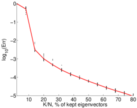
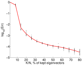
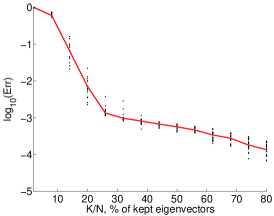
We perform simulations on a 1D grid of points, with impedance of various smoothness and contrast . The result of the compressive wave computation is an approximate discrete solution at a fixed time step of the exact solution of the discretized wave equation.
The performance of the algorithm is evaluated using the recovery error in space and at several time steps for uniformly distributed in , where . The final time is evaluated such that , so that the initial spike at propagates over the whole domain. This error is averaged among a large number of random sets of eigenvectors
| (37) |
Each set is drawn at random using the procedure described in Section 4.1.
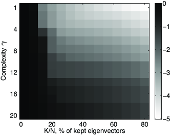
This error depends on the sub-sampling factor , where is the number of computed eigenvectors, and on the impedance of the medium. Numerical evaluation of the decay of Err with are performed for two toy models of acoustic media that could be relevant in seismic settings: smooth with an increasing number of oscillations, and piecewise smooth with an increasing number of discontinuities. For each test, the initial condition is a narrow gaussian bump of standard deviation .
Smooth oscillating medium.
A uniformly smooth impedance parameterized by the number of oscillations is defined as
| (38) |
The contrast is also increased linearly with the complexity of the medium, according to .
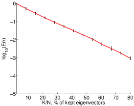
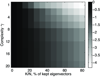
Figure 1 shows how the recovery error scales with complexity of the medium and the number of eigenvectors . For media with moderate complexity, one can compute an accurate solution with to eigenvectors.
 |
|
|
 |
Piecewise smooth medium.
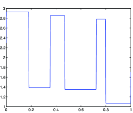
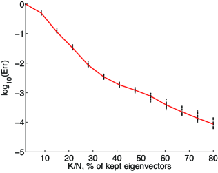
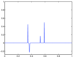
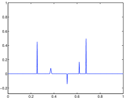
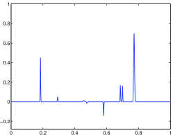
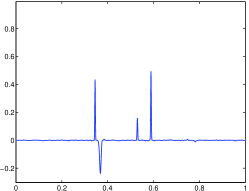
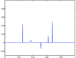
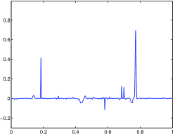
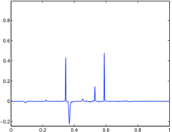
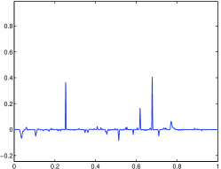
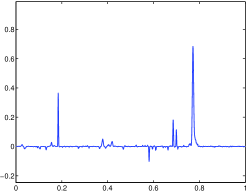
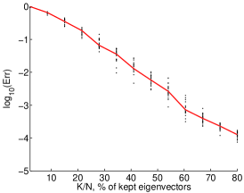
Jump discontinuities in the impedance reflect the propagating spikes and thus deteriorate the sparsity of the solution when increases, as shown on Figure 2, top row. Figure 2 shows that compressive wave computation is able to recover the position of the spikes with roughly to eigenvectors.
 |
 |
| Speed |
|
|
|
|
|
|---|---|---|---|
|
|
|
|
|
|
|
|
|
|
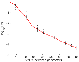
To quantify more precisely the recovery performance, we consider a family of piecewise smooth media parameterized by its number of step discontinuities . The contrast is also increased linearly with the complexity of the medium. The discontinuities are uniformly spread over the spatial domain . The piecewise smooth impedance is slightly regularized by a convolution against a Gaussian kernel of standard deviation . This tends to deteriorate the sparsity of the solution when increases, but helps to avoid numerical dispersion due to the discretization of the Laplacian. Figure 3 shows how the recovery error scales with complexity of the medium and the number of eigenvectors.
 |
|
|
 |
5.2 Compressive Reverse-Time Migration
In this example, we consider an idealized version of the inverse problem of reflection seismology, where wavefield measurements at receivers are used to recover some features of the unknown impedance . Our aim is to show that compressive wave computation offers significant memory savings in the implementation of a specific adjoint-state formulation that we call snapshot reverse-time migration.
Review of 1D reverse-time migration.
We will assume a one-dimensional setup as in the rest of this paper, i.e.,
| (39) |
with a known localized initial condition , , and over a domain sufficiently large that the choice of boundary conditions does not matter. The coordinate plays the role of depth. As in classical treatments of reflection seismology, the squared impedance is perturbed about a smooth, known reference medium , as
where the high-frequency perturbation has the interpretation of “reflectors”. The wave equation is then linearized as
| (40) |
where the incoming field solves the wave equation in the unperturbed medium . An important part of the seismic inversion problem—the “linearized problem”—is to recover from some partial knowledge of , interpreted as solving (40). We will assume the availability of snapshot data, i.e., the value of and at some fixed time ,
possibly restricted in space to a region where the waves are reflected, by opposition to transmitted. We then let for the forward, or modeling operator, to be inverted:
| (41) |
A more realistic seismic setup would be to assume the knowledge of for positive , but the step of going from to , or vice-versa, is a depth-to-time conversion that should present little numerical difficulty. While assuming trace data would give rise to an adjoint-state wave equation with a right-hand side, working with snapshot data has the advantage of casting the adjoint-state equation as a final-value problem without right-hand side.
More precisely, a simple argument of integration by parts (reproduced in the Appendix) shows that the operator in (41) is transposed as
| (42) |
where solves the adjoint-state equation
| (43) |
with final condition
(notice the swap of and , and the minus sign.)
In nice setups, the action of , or for short, called imaging operator, is kinematically equivalent to that of the inverse in the sense that the singularities of are in the same location as those of . In other words the normal operator is pseudodifferential. We also show in the Appendix that is the negative Frechet derivative of a misfit functional for snapshot data, with respect to the medium , in the tradition of adjoint-state methods [48]. Hence applying the imaging operator is a useful component of solving the full inverse problem.
A standard timestepping method is adequate to compute (42); the adjoint wave equation is first solved until time , then both and are evolved together by stepping forward in time and accumulating terms in the quadrature of (42). However, this approach is not without problems:
-
•
The CFL condition restricting the time step for solving the wave equation is typically smaller than the time gridding needed for computing an accurate quadrature of (42). The potential of being able to perform larger, upscaled time steps is obvious.
-
•
The backward-then-forward technique just discussed assumes time-reversibility of the equation in (or conversely of the equation in ), a condition that is not always met in practice, notably when the wave equation comes with either absorbing boundary conditions or an additional viscoelastic term. For non-reversible equations, computation of (42) comes with a big memory overhead due to the fact that one equation is solved from to , while the other one is solved from to . One naive solution is to store the whole evolution; a more sophisticated approach involves using checkpoints [57], where memory is traded for CPU time, but still does not come close to the “working storage” in the time-reversible case. In this context, it would be doubly interesting to avoid or minimize the penalty associated with time stepping.
Numerical validation of compressive reverse time migration.
As a proof of concept, we now show how to perform snapshot reverse-time migration (RTM) without timestepping in the case of the reversible wave equation, on a 1D grid of points. The approach here is simply to compute independently each term of a quadrature of (42) using the compressive wave algorithm for and . We leave to a future project the question of dealing with 2D and 3D non-reversible examples, but we are confident that most of the ideas will carry through.
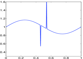
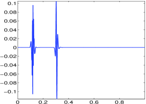
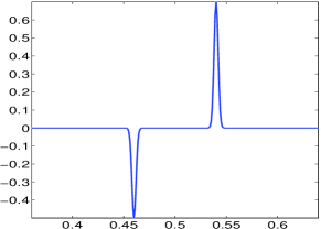
The smooth medium is defined as in (38) with (one oscillation) and a contrast . The reflectors is a sum of two Gaussian bumps of standard deviation and amplitude respectively and , see figure 4, top row.
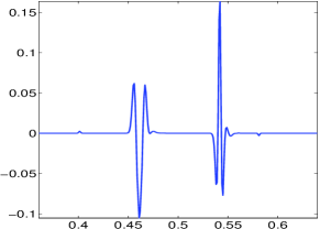
We first compute the input and of the RTM by computing the solution of the wave equation in the perturbed medium , and then evaluate and . The initial condition is a second derivative of a Gaussian of standard deviation . This simulates seismic observations at time , see figure 4, top row.
The algorithm proceeds by computing approximations and of the forward and backward propagations and at equispaced times . These approximations are computed for each independently, without time stepping, by using the compressive algorithm with a small set of eigenvectors. The RTM estimation of the residual is obtained by discretizing (42)
where the derivative is computed using finite differences.
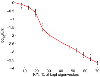
The success of compressive RTM computations is measured using an error measure obtained similarly to (37) by averaging over several randomizations for the sets of eigenvectors
where is the RTM estimation obtained with the full set of eigenvectors.
Figure 4, bottom row, displays the decay of with the number of eigenvectors used for the compressive computations. This shows that roughly of eigenvectors are needed to reach 1 digit of accuracy, and to reach 2 digits of accuracy.
Note that this simple RTM method cannot be expected to recover the original accurately, mainly because we have not undone the action of the normal operator in the least-square treatment of the linearized problem.
Also note that the compressive algorithm was run “as is”, without any decomposition of the initial condition, or split of the time interval over which each simulation is run, as in Section 4.3.
 |
 |
 |
 |
| (zoom) | (zoom) |
 |
6 Discussion
A number of questions still need to be addressed, from both a mathematical and a practical viewpoints.
-
•
Number of eigenvectors. While it is easy to check the accuracy of a compressive solver relative to a standard scheme, an important question is a posteriori validation without comparison to an expensive solver. Were enough eigenvectors sampled? One way to answer this question could be to compare simulation results to those of a coarse-grid standard finite difference scheme. Another possibility is to check for convergence in , as the recovered solution stabilizes as more and more eigenvectors are added. To the best of our knowledge compressed sensing theory does not yet contain a theoretical understanding of a posteriori validation, though.
-
•
Two and three-dimensional media. Passing to a higher-dimensional setting will require using adequate bases for the sparsity of wavefields. Curvelets is one choice, and wave atoms is another one, as both systems were shown to provide to boundedness for all , of the wave equation Green’s functions in media [10, 51]. (Wavelets or ridgelets would only provide to boundedness.) The sparsity question for wave equations in simple nonsmooth media, e.g. including one interface, is to our knowledge completely open. The question of incoherence of the eigenfunctions with respect to such systems will be posed scale-by-scale, in the spirit of wavelets vs. Fourier as in [18] for instance. Incoherence or extension questions for generalized eigenfunctions may also be complicated by the presence of infinite-dimensional eigenspaces in unbounded domains.
-
•
Parallel computing. An exciting outlook is that of scaling the compressive approach to clusters of computers where properly preconditioned and domain-decomposed Helmholtz equations are solved in an entirely parallel fashion over . The solver should be parallelized too, and for the iterative schemes considered the two bottleneck operations are those of applying the incomplete matrix of eigenvectors and its transpose. For reverse-time migration where several times need to be considered, an outstanding question is that of being able to reliably predict the location of large basis coefficients at time from the knowledge of wavefields already solved for at neighboring times and . Note that the advocated “snapshot” variant of reverse-time migration in Section 5.2 contains a preliminary time-to-depth conversion step.
-
•
Other equations and random media. Any linear evolution equation that obeys interesting sparsity and incoherence properties can in principle be studied in the light of compressive computing. This includes the heat equation in simple media; and possibly also the (one-particle) Schrödinger equation in smooth potentials when a bound on wave numbers of the kind is assumed, where is Planck’s constant. Interestingly, the compressive method also makes sense for mildly random media as the reconstruction empirically filters out the trailing “coda” oscillations when they follow behind a coherent wavefront.
Appendix A Additional proofs
Complement to the proof of Theorem 6.
In order to justify (33), consider the quantity
where is adequately regularized in the sense of Lemma 1, but still solves the equation with . Then by point 1 of Lemma 1, makes sense, and
The inhomogeneous Gronwall inequality666If , then , and vice-versa with in both equations instead of . can be applied and yields
| (44) |
where
We can now invoke the different points of Lemma 1. Points 2 and 3, in conjunction with uniform boundedness of and over , allow to conclude that for some constant . By points 4 and 5, the second term in the right-hand side of equation (44) tends pointwise to zero as . Hence by point 2 we have ; and the first term in the right-hand side of equation (44) is handled again by points 4 and 5. The inequality obtained in the limit is
which is what we sought to establish.
Complement to the proof of Theorem 7.
Let us show that (34) holds when and not just . Let be a regularization of , in the usual sense. Define through
where solves the Sturm-Liouville problem with the un-regularized . Then a short calculation shows that
The ratio of sine squared can be recast in terms of a familiar quantity:
The same result follows from a similar formula with cosines in case . Consider now two different frequencies , , and integrate to get
The first term is bounded by , which tends to Var as by point 5 of Lemma 1. The second integral can be compared to by studying
All four factors , , and are bounded and bounded away from zero, by Theorem 6 for and point 3 of Lemma 1 for and . Point 2 of Lemma 1 then implies that . We have already argued in the proof of Theorem 6 that . The limiting inequalities are (34), as desired.
Proof of Proposition 4
Let , where , and let . The basic heuristic is that, even if the probability of drawing a given measurement decreases by a factor which may be less than 1, this effect is at least more than offset by sampling a correspondingly larger number of measurements, namely instead of .
First, let us see why the accuracy bound (8) still holds if we increase the probability for any particular to be included in the list .777Interestingly, the statement that the accuracy of recovery is improved by adding measurements to the minimization problem, is in general false. It is only the error bound that does not degrade. In our context, assume for the moment that
| (45) |
uniformly over . Then we may reduce this setup to a situation where all by a rejection sampling procedure, where each is further labeled as primary, or “accepted”, with probability , and labeled as secondary, or “rejected”, otherwise. The set of primary measurements alone would be adequate to call upon the general theory; passing to obvious linear algebra notations the corresponding constraints are denoted as where satisfies the -RIP with high probability. Adding the secondary measurements cannot fundamentally hurt the recovery of minimization, because the constraints become
for some , hence in particular include . This latter “tube” condition, together with the cone condition that should be minimized, suffice to obtain the recovery estimate on as was shown in [12]. Adding a compatible constraint involving only decreases the feasibility set, hence does not alter the recovery estimate.
Second, it remains to show (45). An event such as refers to the result of a sequential sampling of objects among , without replacement, and according to a certain distribution, either or . This setup is different that the one considered in the classical papers on compressed sensing. It is shown below that
| (46) |
in the uniform case, and
| (47) |
in the nonuniform case. In order for to be greater than as in equation (45), it suffices therefore that , which proves the proposition.
The following proof of (46) and (47) is due to Paul Rubin, who kindly allowed us to reproduce the argument here.
In the case of uniform probabilities, write for short. Denote by the set of drawn during the first iterations. By Bayes theorem applied to a sequence of nested (random) events, we have
The factors telescope in this product, with the result that , hence as desired.
In the case of nonuniform probabilities , consider the quantity
The are themselves random variables, since they depend on the history of sampling up to step . Denote by one realization of , and the corresponding realization of the random process . Then the reasoning essentially proceeds as previously, only by induction on . First, . Assume . Then
We claim that
| (48) |
To justify this inequality, write the sequence of equivalences
The last inequality is obviously true. Therefore
Because this bound is uniform over , it is easy to see that the same inequality holds when the conditioning is on instead of being on .888Indeed, if a random event is the disjoint union , and for all , then as well. This fact is a simple application of Bayes’s theorem: .
We conclude by writing
Proof and discussion of equation (42)
In this proof, a subscript denotes a time differentiation. Consider the following quantity,
where solves (40), and solves (43) with final data not necessarily equal to . Because of (43), this integral is zero. Two integrations by parts in and reveal that
The boundary terms in have been put to zero from assuming, for instance, free-space propagation. In the first two terms, we can use , and recognize that and . For the last term, we may use (40). The result is
On the left, we recognize , where the inner product is in . The right-hand-side is a linear functional of , from to , hence we identify
as required.
Notice that this formula for the adjoint operator is motivated by a standard optimization argument that we now reproduce. Consider the misfit functional for the data , defined as
and under the constraint that solves the original wave equation (39). Then the form of is inspired by the negative Frechet derivative . In order to see this, we can define a dual variable corresponding to the constraint (39), dual variables and corresponding to the initial conditions for , and write the Lagrangian
The same integrations by parts as earlier give
The Frechet derivatives of with respect to , , and reveal the adjoint-state equations:
The derivative of with respect to gives the desired formula
The derivatives with respect to and , replicate the constraints, and finally the derivatives with respect to and are not interesting because they involve , , which do not play a role in the expression of .
Notice that the final conditions for involve the predicted wavefields and . If we put however, and is smooth, then . In that case, essentially no reflections occur and the wavefields , are zero at time , in the region of interest where the data lies. It is only when making corrections to the guess that the predicted wavefields are important in the final condition for .
References
- [1] F. V. Atkinson. Wave propagation and the bremmer series. J. Math. Anal. and Appl., 1:255, 1960.
- [2] Z. Bai, J. Demmel, J. Dongarra, A. Ruhe, and H. van der Vorst. Templates for the Solution of Algebraic Eigenvalue Problems: A Practical Guide. SIAM, Philadelphia, PA, 2000.
- [3] A. Bamberger, G. Chavent, and P. Lailly. Etude mathématique et numérique d’un problème inverse pour l’équation des ondes à une dimension. Rapport IRIA-Laboria no. 226, 1977.
- [4] A. Bamberger, G. Chavent, and P. Lailly. About the stability of the inverse problem in 1-d wave equations: application to the interpretation of seismic profiles. Applied Math. and Optim., 5(1):1–47, 1979.
- [5] R. Barrett, M. Berry, T. F. Chan, J. Demmel, J. Donato, J. Dongarra, V. Eijkhout, R. Pozo, C. Romine, and H. Van der Vorst. Templates for the Solution of Linear Systems: Building Blocks for Iterative Methods, 2nd Edition. SIAM, Philadelphia, PA, 1994.
- [6] G. Beylkin, R. Coifman, and V. Rokhlin. Fast wavelet transforms and numerical algorithms. Commun. on Pure and Appl. Math., 44:141–183, 1991.
- [7] T. Blumensath and M. E. Davies. Gradient pursuits. IEEE Trans. Signal Proc., 56(6):2370–2382, 2008.
- [8] S. Boyd and L. Vandenberghe. Convex Optimization. Cambridge University Press, New York, New York, 2004.
- [9] K. Bredies and D. A. Lorenz. Iterative soft-thresholding converges linearly. submitted, 2007.
- [10] E. Candès and L. Demanet. The curvelet representation of wave propagators is optimally sparse. Commun. on Pure and Appl. Math., 58(11):1472–1528, 2005.
- [11] E. Candès, L. Demanet, D. Donoho, and L. Ying. Fast discrete curvelet transforms. Multiscale Modeling & Simulation, 5(3):861–899, 2006.
- [12] E. Candès, J. Romberg, and T. Tao. Signal recovery from incomplete and inaccurate measurements. Commun. on Pure and Appl. Math., 59(8):1207?–1223, 2005.
- [13] E. Candès, J. Romberg, and T. Tao. Robust uncertainty principles: Exact signal reconstruction from highly incomplete frequency information. IEEE Trans. Info. Theory, 52(2):489–509, 2006.
- [14] E. Candès and T. Tao. Near-optimal signal recovery from random projections: Universal encoding strategies? IEEE Trans. Info. Theory, 52(12):5406–5425, 2006.
- [15] E. J. Candes, M. B. Wakin, and S. P. Boyd. Enhancing sparsity by reweighted L1 minimization. To appear in J. Fourier Anal. Appl., 2007.
- [16] C. Castro and E. Zuazua. Concentration and lack of observability of waves in highly heterogeneous media. Arch. Rat. Mech. Anal., 164:39–72, 2002.
- [17] A. Chambolle. An algorithm for total variation minimization and applications. Journal of Mathematical Imaging and Vision, 20:89–97, 2004.
- [18] S. S. Chen, D.L. Donoho, and M.A. Saunders. Atomic decomposition by basis pursuit. SIAM Journal on Scientific Computing, 20(1):33–61, 1998.
- [19] A. Cohen, W. Dahmen, and R. DeVore. Adaptive wavelet methods for elliptic operator equations: convergence rates. Math. Comp., 70(233):27–75, 2000.
- [20] P. L. Combettes and V. R. Wajs. Gsignal recovery by proximal forward-backward splitting. SIAM Journal on Multiscale Modeling and Simulation, 4(4), 2005.
- [21] F. Conrad, J. Leblond, and J.P. Marmorat. Boundary control and stabilization of the one-dimensional wave equation. Lecture Notes in control and Inform. Sci., 178:142–162, 1992.
- [22] I. Daubechies, M. Defrise, and C. De Mol. An iterative thresholding algorithm for linear inverse problems with a sparsity constraint. Commun. on Pure and Appl. Math., 57:1413–1541, 2004.
- [23] R. Dautray and J.L. Lions. Mathematical Analysis and Numerical Methods for Science and Technology. Springer-Verlag, 1990.
- [24] L. Demanet and L. Ying. Discrete symbol calculus. submitted, 2008.
- [25] L. Demanet and L. Ying. Wave atoms and time upscaling of wave equations. To appear in Numer. Math., 2008.
- [26] R. A. DeVore. Nonlinear approximation. Acta Numerica, 7:51–150, 1998.
- [27] R. A. DeVore and G. G. Lorentz. Constructive approximation, volume 303 of Grundlehren der math. Wissenschaften. Springer, 1993.
- [28] D. Donoho. Compressed sensing. IEEE Trans. Info. Theory, 52(4):1289–1306, 2006.
- [29] D. L. Donoho and P. B. Stark. Uncertainty principles and signal recovery. SIAM J. of Appl. Math., 49(3):906–931, June 1989.
- [30] D. L. Donoho and Y. Tsaig. Fast solution of -norm minimization problems when the solution may be sparse. to appear in Journal of Mathematical Imaging and Vision, 2006.
- [31] W. Yin E. T. Hale and Y. Zhang. A fixed-point continuation method for l1-regularized minimization with applications to compressed sensing. CAAM Technical Report TR07-07, 2008.
- [32] B. Efron, T. Hastie, I. Johnstone, and T. Tibshirani. Least angle regression. Annals of Statistics, 32(2):407–499, 2004.
- [33] B. Engquist, S. Osher, and S. Zhong. Fast wavelet based algorithms for evolution equations. SIAM J. Sci. Comput., 15(4):755–775, 1994.
- [34] Y. Erlangga and R. Nabben. Multilevel projection-based nested krylov iteration for boundary value problems, 2008.
- [35] M. Figueiredo and R. Nowak. An EM Algorithm for Wavelet-Based Image Restoration. IEEE Trans. Image Proc., 12(8):906–916, 2003.
- [36] M. A. T. Figueiredo, R. D. Nowak, and S. J. Wright. Gradient projection for sparse reconstruction: Application to compressed sensing and other inverse problems. IEEE Journal of Selected Topics in Signal Processing, 1(4):586–598, 2007.
- [37] J-P. Fouque, J. Garnier, G. Papanicolaou, and K. Solna. Wave Propagation and Time Reversal in Randomly Layered Media, volume 56 of Stochastic Modelling and Applied Probability. Springer, 2007.
- [38] I. F. Gorodnitsky and B. D. Rao. Sparse signal reconstruction from limited data using FOCUSS: a re-weighted minimum norm algorithm. IEEE Trans. Image Proc., 45(3):600–616, March 1997.
- [39] P. W. Jones, M. Maggioni, and R. Schul. Universal local parametrizations via heat kernels and eigenfunctions of the laplacian. Submitted, 2008.
- [40] R.M. Lewis and W.W. Symes. On the relation between the velocity coefficient and boundary value for solutions of the one-dimensional wave equation. Inverse Problems, 7(35):597–631, 1991.
- [41] T. Lin and F. Herrmann. Compressed wavefield extrapolation. Geophysics, 72(5):77–93, 2007.
- [42] J. L. Lions and E. Magenes. Non-Homogeneous Boundary Value Problems and Applications. Stochastic Modelling and Applied Probability. Springer-Verlag, 1972.
- [43] S. Mallat. A wavelet tour of signal processing, 3rd edition. Academic Press, San Diego, USA, 2008.
- [44] Y. Meyer. Wavelets and Operators. Analysis at Urbana, London Math. Soc. Lecture Notes Series 137. Cambridge University Press, 1989.
- [45] D. Needell and J. A. Tropp. Cosamp: Iterative signal recovery from incomplete and inaccurate samples. to appear in Appl. Comp. Harmonic Anal., 2008.
- [46] Y. Nesterov. Smooth minimization of non-smooth functions. Math. Program., 103(1, Ser. A):127–152, 2005.
- [47] H. Owhadi and L. Zhang. Numerical homogenization of the acoustic wave equations with a continuum of scales, 2008.
- [48] R. E. Plessix. A review of the adjoint-state method for computing the gradient of a functional with geophysical applications. Geophysical Journal International, 167(9):495–503, 2006.
- [49] M. Rudelson and R.Vershynin. On sparse reconstruction from fourier and gaussian measurements. Commun. on Pure and Appl. Math., 61(8):1025–1045, 2008.
- [50] F. Santosa and W. W. Symes. Linear inversion of band-limited reflection seismograms. SIAM Journal on Scientific and Statistical Computing, 7(4):1307–1330, 1986.
- [51] H. F. Smith. A parametrix construction for wave equations with coefficients. Ann. Inst. Fourier (Grenoble), 48:797–835, 1998.
- [52] H. F. Smith. Spectral cluster estimates for metrics. Amer. J. Math., 128:1069–1103, 2006.
- [53] C. D. Sogge. Eigenfunction and bochner-riesz estimates on manifolds with boundary. Math. Research Letters, 9:205–216, 2002.
- [54] J.-L. Starck, M. Elad, and D.L. Donoho. Redundant multiscale transforms and their application for morphological component analysis. Advances in Imaging and Electron Physics, 132, 2004.
- [55] C. C. Stolk. PhD thesis, On the Modeling and Inversion of Seismic Data. PhD thesis, Utrecht University, 2000.
- [56] W. W. Symes. Transparency of one-dimensional acoustic media of bounded variation. TRIP technical report, 1985.
- [57] W. W. Symes. Reverse time migration with optimal checkpointing. Geophysics, 72(5):213–221, 2007.
- [58] W. Yin, S. Osher, J. Darbon, and D. Goldfarb. Bregman iterative algorithms for compressed sensing and related problems. CAAM TR07-13, 2007.
- [59] M. Zhu and T. Chan. An efficient primal-dual hybrid gradient algorithm for total variation image restoration. UCLA CAM Report 08-34, 2007.
- [60] W. Ziemer. Weakly Differentiable Functions. Graduate texts in Mathematics. Springer-Verlag, 1989.
- [61] E. Zuazua. Exact controllability for semilinear wave equations in one space dimension. Annales I.H.P. section C, 10(1):109–129, 1993.
- [62] E. Zuazua. Propagation, observation, and control of waves approximated by finite difference methods. SIAM Rev., 47(2):197–243, 2005.