End-monomer Dynamics in Semiflexible Polymers

Michael Hinczewski , Xaver Schlagberger , Michael Rubinstein ,
Oleg Krichevsky , and Roland R. Netz
Feza Gürsey Research Institute, TÜBITAK - Bosphorus University, Çengelköy 34684, Istanbul, TurkeyPhysics Department, Technical University of Munich, 85748 Garching, GermanyDepartment of Chemistry, University of North Carolina, Chapel Hill, NC 27599-3290, USAPhysics Department, Ben-Gurion University, Beer-Sheva 84105, Israel
Abstract

Spurred by an experimental controversy in the literature, we investigate the end-monomer dynamics of semiflexible polymers through Brownian hydrodynamic simulations and dynamic mean-field theory. Precise experimental observations over the last few years of end-monomer dynamics in the diffusion of double-stranded DNA have given conflicting results: one study indicated an unexpected Rouse-like scaling of the mean squared displacement (MSD) r2(t)t1/2similar-todelimited-⟨⟩superscript𝑟2𝑡superscript𝑡12\langle r^{2}(t)\rangle\sim t^{1/2} at intermediate times, corresponding to fluctuations at length scales larger than the persistence length but smaller than the coil size; another study claimed the more conventional Zimm scaling r2(t)t2/3similar-todelimited-⟨⟩superscript𝑟2𝑡superscript𝑡23\langle r^{2}(t)\rangle\sim t^{2/3} in the same time range. Using hydrodynamic simulations, analytical and scaling theories, we find a novel intermediate dynamical regime where the effective local exponent of the end-monomer MSD, α(t)=dlogr2(t)/dlogt𝛼𝑡𝑑superscript𝑟2𝑡𝑑𝑡\alpha(t)=d\log\langle r^{2}(t)\rangle/d\log t, drops below the Zimm value of 2/3 for sufficiently long chains. The deviation from the Zimm prediction increases with chain length, though it does not reach the Rouse limit of 1/2. The qualitative features of this intermediate regime, found in simulations and in an improved mean-field theory for semiflexible polymers, in particular the variation of α(t)𝛼𝑡\alpha(t) with chain and persistence lengths, can be reproduced through a heuristic scaling argument. Anomalously low values of the effective exponent α𝛼\alpha are explained by hydrodynamic effects related to the slow crossover from dynamics on length scales smaller than the persistence length to dynamics on larger length scales.

1 Introduction

Recent experimental advances using fluorescence correlation spectroscopy [1, 2, 3, 4, 5] have given unprecedented information about the dynamical behavior of large single polymer molecules in solution, in particular the small-scale kinetics of individual monomers inaccessible to traditional techniques like dynamic light scattering. One of the first studies along this direction yielded an unexpected result. Shusterman et al. [2] observed the random motion of a single labeled monomer at the end of a long double-stranded DNA molecule, and found evidence of an “intermediate Rouse regime”: the mean squared displacement (MSD) followed a scaling r2(t)t1/2proportional-todelimited-⟨⟩superscript𝑟2𝑡superscript𝑡12\langle r^{2}(t)\rangle\propto t^{1/2} for a wide time range corresponding to polymer motion at length scales smaller than the coil size Rgsubscript𝑅𝑔R_{g} but larger than the persistence length lpsubscript𝑙𝑝l_{p}. This agrees with the free-draining Rouse model for a polymer which neglects hydrodynamic interactions mediated by flow fields arising from the monomers moving through the solvent. Such a result contradicts the conventional wisdom for flexible polymers, which states that these hydrodynamic interactions play a crucial role in polymer dynamics in dilute solutions and give rise to non-draining behavior that is qualitatively described by the Zimm theory, which predicts r2(t)t2/3proportional-todelimited-⟨⟩superscript𝑟2𝑡superscript𝑡23\langle r^{2}(t)\rangle\propto t^{2/3} [6, 7]. Though double-stranded DNA is a semiflexible polymer (having a persistence length lp50100subscript𝑙𝑝50100l_{p}\approx 50-100 nm much larger than the width 2absent2\approx 2 nm), the expectation for kinetics at scales larger than lpsubscript𝑙𝑝l_{p} is that it behaves like a non-draining flexible polymer. Thus the apparent absence of hydrodynamic effects is quite surprising, and the intermediate Rouse regime does not fit into established theories of the dynamics of flexible polymers in dilute solutions, though recently there has been an attempt to explain its existence through a theory exhibiting time-dependent hydrodynamic screening [8]. On the other hand, a new experimental study by Petrov et. al. [5] on the same system did not seem to show the Rouse regime, and its results were interpreted to be generally consistent with the dynamics predicted by the Zimm theory. Arguably the dynamics of a semiflexible polymer such as DNA may be expected to differ from that of flexible polymers. However, with the exception of the Harnau, Winkler, Reineker (HWR) model [9], other established theories of the dynamics of semi-flexible polymers [10, 11] treat only the range of displacements smaller than the persistence length r2(t)<lp2delimited-⟨⟩superscript𝑟2𝑡superscriptsubscript𝑙𝑝2\langle r^{2}(t)\rangle<l_{p}^{2}.

To help resolve the controversy over the dynamics of semiflexible polymers on intermediate length scales lp2<r2(t)<L2superscriptsubscript𝑙𝑝2delimited-⟨⟩superscript𝑟2𝑡superscript𝐿2l_{p}^{2}<\langle r^{2}(t)\rangle<L^{2}, we study the end-monomer behavior of semiflexible chains in dilute solutions using two approaches: dynamic mean-field theory (MFT) that includes hydrodynamics with the pre-averaging approximation, and Brownian hydrodynamics simulations without the pre-averaging approximation. The end-monomer MSD, diffusion constants, and longest relaxation times from the two approaches agree closely with each other. While the hydrodynamic pre-averaging MFT method is similar to that of HWR in Ref. 9, we have improved the approximation by taking into account the full hydrodynamic interaction matrix in the Langevin equation, and not just the diagonal contribution. This leads to much better agreement between the MFT and the simulation data: compared with the earlier version, the improved MFT is 10–65% closer to the mean-square displacement r2(t)delimited-⟨⟩superscript𝑟2𝑡\langle r^{2}(t)\rangle of the end monomer obtained by simulations for time scales shorter than the longest relaxation time of the chain, and reduces the discrepancy in the effective local exponent α(t)=dlogr2(t)/dlogt𝛼𝑡𝑑superscript𝑟2𝑡𝑑𝑡\alpha(t)=d\log\langle r^{2}(t)\rangle/d\log t in this time range, which is underestimated by as much as 10% using the earlier method. Thus we can confidently extend the MFT to larger chain lengths L𝐿L that are inaccessible to simulation. For these chains we find an intermediate dynamical regime where the continuously varying effective local exponent of the end-monomer MSD, α(t)𝛼𝑡\alpha(t), drops below 2/3, and its difference from this Zimm value increases with L𝐿L. The existence of this regime and the qualitative trends of α(t)𝛼𝑡\alpha(t) with changing L𝐿L and lpsubscript𝑙𝑝l_{p} are verified independently through a heuristic scaling argument. However even at the largest chain lengths examined, comparable to or longer than the experimentally studied chains of Refs. 2 and 5, the effective exponent α(t)𝛼𝑡\alpha(t) does not reach the Rouse limit of 1/2. Comparison with the experimental MSD data of Ref. 2 reveals two interesting results: the MFT accurately describes the long-time diffusion behavior, related to the large-scale dynamics of the chain; however at shorter times it underestimates the extent of the MSD. As we show in this paper, the same sub-Zimm scaling of the MSD is also contained in the HWR theory that was used to successfully fit the data of Ref. 5. So the question is not whether an intermediate sub-Zimm scaling regime exists, but rather how large that regime is and how small are the intermediate exponents. The remaining discrepancy between theory and experiment discussed in this paper highlights the importance of additional dynamical degrees of freedom absent in the worm-like chain model used as the starting point for the theoretical description of DNA or some shortcomings in the current analysis of FCS data.

The paper is organized as follows: in Sec. 2 we give a heuristic scaling argument that captures the basic properties of the intermediate dynamical regime; in Sec. 3 we describe the details of the Brownian dynamics simulations; in Sec. 4 we give an overview of the mean-field model for semiflexible polymers and the pre-averaging approximation used to determine its behavior in solution; in Sec. 5 we compare the simulation, MFT, and heuristic results, together with the experimental data. The dynamical regimes exhibited in these results are examined through asymptotic scaling analysis in Sec. 6, and placed in the context of earlier theories. Finally Sec. 7 summarizes the main points of the paper. Additional material, extending the mean-field model of Sec. 4 to extensible worm-like chains, is provided in Appendix A. Mathematical details of an analytical approximation used in Sec. 6 are given in Appendix B.

2 Heuristic Scaling Argument
Refer to caption
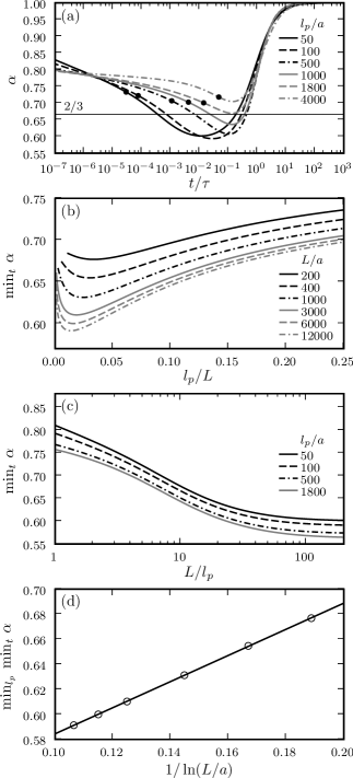
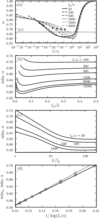
Figure 1: Results of the heuristic scaling argument described in Sec. 2. (a) The effective exponent α=dlogr2(t)/dlogt𝛼𝑑superscript𝑟2𝑡𝑑𝑡\alpha=d\log\langle r^{2}(t)\rangle/d\log t versus t/τ𝑡𝜏t/\tau for polymers of diameter 2a2𝑎2a, contour length L=12000a𝐿12000𝑎L=12000a, and various persistence lengths lp=50a4000asubscript𝑙𝑝50𝑎4000𝑎l_{p}=50a-4000a. The dot along each α(t)𝛼𝑡\alpha(t) curve marks α(τp)𝛼subscript𝜏𝑝\alpha(\tau_{p}). The time scales τ𝜏\tau and τpsubscript𝜏𝑝\tau_{p} are defined in the text. (b) The minimum value of α𝛼\alpha over all t𝑡t versus lp/Lsubscript𝑙𝑝𝐿l_{p}/L for several L=200a12000a𝐿200𝑎12000𝑎L=200a-12000a. (c) The minimum value of α𝛼\alpha over all t𝑡t versus L/lp𝐿subscript𝑙𝑝L/l_{p} for several lp=50a1800asubscript𝑙𝑝50𝑎1800𝑎l_{p}=50a-1800a. (d) The circles show the minimum value of α𝛼\alpha in each of the curves in panel (b), plotted as a function of 1/ln(L/a)1𝐿𝑎1/\ln(L/a). Superimposed is a straight-line fit to the data points, minlpmintα0.48+1.04/ln(L/a)subscriptsubscript𝑙𝑝subscript𝑡𝛼0.481.04𝐿𝑎\min_{l_{p}}\min_{t}\alpha\approx 0.48+1.04/\ln(L/a).
Refer to caption
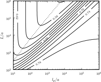
Figure 2: The contours show the minimum value of the effective exponent α(t)=dlogr2(t)/dlogt𝛼𝑡𝑑superscript𝑟2𝑡𝑑𝑡\alpha(t)=d\log\langle r^{2}(t)\rangle/d\log t over all t𝑡t calculated using the heuristic scaling argument in Sec. 2 for chains of diameter 2a2𝑎2a, total length L𝐿L, and persistence length lpsubscript𝑙𝑝l_{p}. The interval between contours is 0.02. The dotted line indicates the minimum value of mintαsubscript𝑡𝛼\min_{t}\alpha over lp/asubscript𝑙𝑝𝑎l_{p}/a for a given L/a𝐿𝑎L/a.

Certain qualitative features of the intermediate dynamical regime for semiflexible polymers can be derived from a scaling argument similar to the one that is typically used to understand subdiffusive motion in the Rouse or Zimm models [12]. In our heuristic scaling, we assume that at time scales t𝑡t the diffusion of the polymer is characterized by the coherent motion of a section with contour length (t)𝑡\ell(t). The MSD of a monomer during this time t𝑡t has two limiting subdiffusive behaviors depending on the magnitude of (t)𝑡\ell(t). For (t)lpmuch-less-than𝑡subscript𝑙𝑝\ell(t)\ll l_{p}, where the local stiffness of the polymer plays the key role, the MSD r2(t)delimited-⟨⟩superscript𝑟2𝑡\langle r^{2}(t)\rangle is dominated by transverse chain fluctuations and thus r2(t)(t)3/lpsimilar-todelimited-⟨⟩superscript𝑟2𝑡superscript𝑡3subscript𝑙𝑝\langle r^{2}(t)\rangle\sim\ell(t)^{3}/l_{p} [10, 11, 13, 14, 15, 12]. For (t)lpmuch-greater-than𝑡subscript𝑙𝑝\ell(t)\gg l_{p}, the MSD can be estimated as r2(t)ree2((t))similar-todelimited-⟨⟩superscript𝑟2𝑡subscriptsuperscript𝑟2ee𝑡\langle r^{2}(t)\rangle\sim r^{2}_{\text{ee}}(\ell(t)), where ree2()subscriptsuperscript𝑟2eer^{2}_{\text{ee}}(\ell) is the mean squared end-to-end distance of a polymer of contour length \ell. For a semiflexible chain with persistence length lpsubscript𝑙𝑝l_{p} this is given by:

ree2()=2lp2lp2(1e/lp).subscriptsuperscript𝑟2ee2subscript𝑙𝑝2superscriptsubscript𝑙𝑝21superscript𝑒subscript𝑙𝑝r^{2}_{\text{ee}}(\ell)=2l_{p}\ell-2l_{p}^{2}(1-e^{-\ell/l_{p}})\,. (1)

Thus the total intramolecular contribution to the MSD, rintra2(t)delimited-⟨⟩subscriptsuperscript𝑟2intra𝑡\langle r^{2}_{\text{intra}}(t)\rangle, can be written in a heuristic form which smoothly interpolates between these two limits:

rintra2(t)=C1[{ree2((t))}ϕ1+C1{(ree2((t)))3/2lp}ϕ1]1/ϕ1.delimited-⟨⟩subscriptsuperscript𝑟2intra𝑡subscript𝐶1superscriptdelimited-[]superscriptsubscriptsuperscript𝑟2ee𝑡subscriptitalic-ϕ1superscriptsubscript𝐶1superscriptsuperscriptsubscriptsuperscript𝑟2ee𝑡32subscript𝑙𝑝subscriptitalic-ϕ11subscriptitalic-ϕ1\langle r^{2}_{\text{intra}}(t)\rangle=C_{1}\left[\{r^{2}_{\text{ee}}(\ell(t))\}^{-\phi_{1}}+C_{1}^{\prime}\left\{\frac{(r^{2}_{\text{ee}}(\ell(t)))^{3/2}}{l_{p}}\right\}^{-\phi_{1}}\right]^{-1/\phi_{1}}\,. (2)

Using the fact that ree2()2subscriptsuperscript𝑟2eesuperscript2r^{2}_{\text{ee}}(\ell)\approx\ell^{2} for lpmuch-less-thansubscript𝑙𝑝\ell\ll l_{p}, one can easily check that Eq. (2) has the appropriate asymptotic limits for small and large (t)𝑡\ell(t), with the crossover occurring at tτp𝑡subscript𝜏𝑝t\approx\tau_{p} where the relaxation time τpsubscript𝜏𝑝\tau_{p} of a persistent segment is defined by ree2((τp))=lp2subscriptsuperscript𝑟2eesubscript𝜏𝑝superscriptsubscript𝑙𝑝2r^{2}_{\text{ee}}(\ell(\tau_{p}))=l_{p}^{2}. We added numerical constants C1,C1O(1)similar-tosubscript𝐶1superscriptsubscript𝐶1O1C_{1},\>C_{1}^{\prime}\sim\text{O}(1) and a crossover exponent ϕ1subscriptitalic-ϕ1\phi_{1} which will be determined from the comparison with numerical data.

In order to close the scaling argument, we write the diffusion relation between spatial and temporal scales

rintra2(t)=6D((t))t,delimited-⟨⟩subscriptsuperscript𝑟2intra𝑡6𝐷𝑡𝑡\langle r^{2}_{\text{intra}}(t)\rangle=6D(\ell(t))t, (3)

in terms of an effective diffusion constant D()𝐷D(\ell) for a polymer section of length \ell. D()𝐷D(\ell) can be estimated from a heuristic formula [16] that compares well with both simulation and experimental DNA results:

D()=C2(Dcylϕ2()+Dcoilϕ2())1/ϕ2,𝐷subscript𝐶2superscriptsuperscriptsubscript𝐷cylsubscriptitalic-ϕ2superscriptsubscript𝐷coilsubscriptitalic-ϕ21subscriptitalic-ϕ2D(\ell)=C_{2}(D_{\text{cyl}}^{\phi_{2}}(\ell)+D_{\text{coil}}^{\phi_{2}}(\ell))^{1/\phi_{2}}\,, (4)

where

Dcyl()=2μ0kBT[log2a+0.312+0.565(2a)0.1(2a)2],Dcoil()=2.22μ0kBTalp.formulae-sequencesubscript𝐷cyl2subscript𝜇0subscript𝑘𝐵𝑇2𝑎0.3120.5652𝑎0.1superscript2𝑎2subscript𝐷coil2.22subscript𝜇0subscript𝑘𝐵𝑇𝑎subscript𝑙𝑝\begin{split}D_{\text{cyl}}(\ell)&=\frac{2\mu_{0}k_{B}T}{\ell}\left[\log\frac{\ell}{2a}+0.312\right.\\ &\qquad\qquad\quad\left.+0.565\left(\frac{2a}{\ell}\right)-0.1\left(\frac{2a}{\ell}\right)^{2}\right]\,,\\ D_{\text{coil}}(\ell)&=\frac{2.22\mu_{0}k_{B}Ta}{\sqrt{l_{p}\ell}}\,.\end{split} (5)

Here 2a2𝑎2a is the diameter of the chain, μ0=1/(6πηa)subscript𝜇016𝜋𝜂𝑎\mu_{0}=1/(6\pi\eta a) is the Stokes mobility of a single sphere of radius a𝑎a, and η𝜂\eta is the viscosity of water. Dcyl()subscript𝐷cylD_{\text{cyl}}(\ell) is the diffusion constant of a stiff cylinder [17], and Dcoil()subscript𝐷coilD_{\text{coil}}(\ell) gives the diffusion constant of an ideal chain in the flexible limit where lpmuch-greater-thansubscript𝑙𝑝\ell\gg l_{p}. We assume lp3/a2much-less-thansuperscriptsubscript𝑙𝑝3superscript𝑎2\ell\ll l_{p}^{3}/a^{2}, so self-avoidance effects can be ignored [18]. For parameter values a=1𝑎1a=1 nm and lp=50subscript𝑙𝑝50l_{p}=50 nm, typical of DNA, these effects are only important at scales greater than 102similar-toabsentsuperscript102\sim 10^{2} μ𝜇\mum, far larger than the chain lengths investigated in the experimental studies discussed above. Eq. (4) is an interpolation between the limiting cases given by Dcyl()subscript𝐷cylD_{\text{cyl}}(\ell) when lpmuch-less-thansubscript𝑙𝑝\ell\ll l_{p} and Dcoil()subscript𝐷coilD_{\text{coil}}(\ell) when lpmuch-greater-thansubscript𝑙𝑝\ell\gg l_{p}. In Ref. 16 the crossover exponent was determined to be ϕ2=3subscriptitalic-ϕ23\phi_{2}=3 and with the definition of Dcyl()subscript𝐷cylD_{\text{cyl}}(\ell) and Dcoil()subscript𝐷coilD_{\text{coil}}(\ell) the constant was fixed at C2=1subscript𝐶21C_{2}=1. In the present context we use ϕ2subscriptitalic-ϕ2\phi_{2} and C2O(1)similar-tosubscript𝐶2O1C_{2}\sim\text{O}(1) as parameters that will be adjusted to fit the numerical data.

The asymptotic Zimm scaling is easily obtained from the expressions written so far: In the flexible regime, for lpmuch-greater-thansubscript𝑙𝑝\ell\gg l_{p}, we have Dcoil(lp)1/2similar-tosubscript𝐷coilsuperscriptsubscript𝑙𝑝12D_{\text{coil}}\sim(\ell l_{p})^{-1/2} and from Eqs. (1) and  (2) we find rintra2lpsimilar-todelimited-⟨⟩subscriptsuperscript𝑟2intrasubscript𝑙𝑝\langle r^{2}_{\text{intra}}\rangle\sim\ell l_{p}. Using rintra2Dtsimilar-todelimited-⟨⟩subscriptsuperscript𝑟2intra𝐷𝑡\langle r^{2}_{\text{intra}}\rangle\sim Dt from Eqs. (3) we thus obtain t2/3/lpsimilar-tosuperscript𝑡23subscript𝑙𝑝\ell\sim t^{2/3}/l_{p} and rintra2t2/3similar-todelimited-⟨⟩subscriptsuperscript𝑟2intrasuperscript𝑡23\langle r^{2}_{\text{intra}}\rangle\sim t^{2/3}, the well-known Zimm scaling for flexible polymers [12]. In the stiff polymer regime, for lpmuch-less-thansubscript𝑙𝑝\ell\ll l_{p}, we have Dcyl1log(/a)similar-tosubscript𝐷cylsuperscript1𝑎D_{\text{cyl}}\sim\ell^{-1}\log(\ell/a) and from Eq. (2) we find rintra23/lpsimilar-todelimited-⟨⟩subscriptsuperscript𝑟2intrasuperscript3subscript𝑙𝑝\langle r^{2}_{\text{intra}}\rangle\sim\ell^{3}/l_{p}. Again using rintra2Dtsimilar-todelimited-⟨⟩subscriptsuperscript𝑟2intra𝐷𝑡\langle r^{2}_{\text{intra}}\rangle\sim Dt we obtain this time (tlplogt)1/4similar-tosuperscript𝑡subscript𝑙𝑝𝑡14\ell\sim(tl_{p}\log t)^{1/4} and thus rintra2t3/4lp1/4log3/4tsimilar-todelimited-⟨⟩subscriptsuperscript𝑟2intrasuperscript𝑡34superscriptsubscript𝑙𝑝14superscript34𝑡\langle r^{2}_{\text{intra}}\rangle\sim t^{3/4}l_{p}^{-1/4}\log^{3/4}t. The MSD scaling of semiflexible polymers has pronounced logarithmic corrections in the stiff polymer regime due to hydrodynamic effects.

To get an expression for the total MSD, r2(t)delimited-⟨⟩superscript𝑟2𝑡\langle r^{2}(t)\rangle, that includes the long-time regime, one must consider also the crossover which occurs near time t=τ𝑡𝜏t=\tau, where (τ)=L𝜏𝐿\ell(\tau)=L, the total contour length of the chain. For tτmuch-greater-than𝑡𝜏t\gg\tau the effective diffusion constant is D(L)𝐷𝐿D(L), and r2(t)6D(L)tdelimited-⟨⟩superscript𝑟2𝑡6𝐷𝐿𝑡\langle r^{2}(t)\rangle\approx 6D(L)t, describing the trivial diffusion of the whole polymer coil. τ𝜏\tau corresponds approximately to the longest relaxation time of the polymer. This crossover is captured by yet another crossover expression,

r2(t)=[rintra2(t)ϕ3+{6D(L)t}ϕ3]1/ϕ3,delimited-⟨⟩superscript𝑟2𝑡superscriptdelimited-[]superscriptdelimited-⟨⟩subscriptsuperscript𝑟2intra𝑡subscriptitalic-ϕ3superscript6𝐷𝐿𝑡subscriptitalic-ϕ31subscriptitalic-ϕ3\langle r^{2}(t)\rangle=\left[\langle r^{2}_{\text{intra}}(t)\rangle^{\phi_{3}}+\{6D(L)t\}^{\phi_{3}}\right]^{1/\phi_{3}}\,, (6)

which gives the correct asymptotic scaling behavior for r2(t)delimited-⟨⟩superscript𝑟2𝑡\langle r^{2}(t)\rangle in all time regimes. In the results below, the exponents ϕ1subscriptitalic-ϕ1\phi_{1}, ϕ2subscriptitalic-ϕ2\phi_{2}, ϕ3subscriptitalic-ϕ3\phi_{3}, and the three constants C1subscript𝐶1C_{1}, C1superscriptsubscript𝐶1C_{1}^{\prime}, C2subscript𝐶2C_{2} in Eqs. (2), (4), and (6) are chosen so that the heuristic scaling argument approximately agrees, for long chain lengths, with the numerical results of the MFT approach described in the next section. The best-fit values are: ϕ1=0.84subscriptitalic-ϕ10.84\phi_{1}=0.84, ϕ2=3.15subscriptitalic-ϕ23.15\phi_{2}=3.15, ϕ3=3.62subscriptitalic-ϕ33.62\phi_{3}=3.62, C1=3.65subscript𝐶13.65C_{1}=3.65, C1=0.66superscriptsubscript𝐶10.66C_{1}^{\prime}=0.66, C2=1.31subscript𝐶21.31C_{2}=1.31.

The full time dependence covering also the non-asymptotic behavior is obtained by equating the expressions for rintra2(t)delimited-⟨⟩subscriptsuperscript𝑟2intra𝑡\langle r^{2}_{\text{intra}}(t)\rangle in Eqs. (2) and (3) and implicitly solving for (t)𝑡\ell(t); we thus calculate rintra2(t)delimited-⟨⟩subscriptsuperscript𝑟2intra𝑡\langle r^{2}_{\text{intra}}(t)\rangle as a function of t𝑡t. Plugging the result for rintra2(t)delimited-⟨⟩subscriptsuperscript𝑟2intra𝑡\langle r^{2}_{\text{intra}}(t)\rangle into Eq. (6) gives the total MSD r2(t)delimited-⟨⟩superscript𝑟2𝑡\langle r^{2}(t)\rangle. The time evolution of r2(t)delimited-⟨⟩superscript𝑟2𝑡\langle r^{2}(t)\rangle can be expressed through the effective exponent α(t)=dlogr2(t)/dlogt𝛼𝑡𝑑superscript𝑟2𝑡𝑑𝑡\alpha(t)=d\log\langle r^{2}(t)\rangle/d\log t. Fig. 1(a) shows α(t)𝛼𝑡\alpha(t) versus t/τ𝑡𝜏t/\tau for chains of total length L=12000a𝐿12000𝑎L=12000a, with various persistence lengths in the range lp=25a4000asubscript𝑙𝑝25𝑎4000𝑎l_{p}=25a-4000a. The dot along each α(t)𝛼𝑡\alpha(t) curve marks α(τp)𝛼subscript𝜏𝑝\alpha(\tau_{p}). There is clearly an intermediate time regime, within the range τp<t<τsubscript𝜏𝑝𝑡𝜏\tau_{p}<t<\tau, where α(t)𝛼𝑡\alpha(t) dips below the Zimm value of 2/3. The minimum value of α(t)𝛼𝑡\alpha(t) over all t𝑡t depends both on L𝐿L and lpsubscript𝑙𝑝l_{p}, as shown in Figs. 1(b) and (c), which plot mintαsubscript𝑡𝛼\min_{t}\alpha versus lp/Lsubscript𝑙𝑝𝐿l_{p}/L for several chain lengths L=100a12000a𝐿100𝑎12000𝑎L=100a-12000a, and mintαsubscript𝑡𝛼\min_{t}\alpha versus L/lp𝐿subscript𝑙𝑝L/l_{p} for several lpsubscript𝑙𝑝l_{p} in the range lp=50a1800asubscript𝑙𝑝50𝑎1800𝑎l_{p}=50a-1800a. The overall variation of mintαsubscript𝑡𝛼\min_{t}\alpha as a function of L/a𝐿𝑎L/a and lp/asubscript𝑙𝑝𝑎l_{p}/a is depicted in the contour diagram of Fig. 2. The deviation from Zimm behavior becomes more prominent with increasing L𝐿L: the time range where α<2/3𝛼23\alpha<2/3 increases, and the values of mintαsubscript𝑡𝛼\min_{t}\alpha decrease. As seen in Fig. 1(c), for fixed lp/asubscript𝑙𝑝𝑎l_{p}/a the decrease in mintαsubscript𝑡𝛼\min_{t}\alpha with L𝐿L eventually saturates for Llpmuch-greater-than𝐿subscript𝑙𝑝L\gg l_{p}. The mintαsubscript𝑡𝛼\min_{t}\alpha curves in Fig. 1(b) all reach a minimum in the range lp/L0.010.04similar-tosubscript𝑙𝑝𝐿0.010.04l_{p}/L\sim 0.01-0.04. The position of the minimum decreases with L𝐿L approximately with the logarithmic dependence lp/L0.013+0.26/log(L/a)subscript𝑙𝑝𝐿0.0130.26𝐿𝑎l_{p}/L\approx-0.013+0.26/\log(L/a). The exponent values at these minima, minlpmintαsubscriptsubscript𝑙𝑝subscript𝑡𝛼\min_{l_{p}}\min_{t}\alpha, also have a nearly linear dependence on 1/log(L/a)1𝐿𝑎1/\log(L/a), as can be seen in Fig. 1(d), where minlpmintαsubscriptsubscript𝑙𝑝subscript𝑡𝛼\min_{l_{p}}\min_{t}\alpha goes from 0.677 at L=200a𝐿200𝑎L=200a to 0.591 at L=12000a𝐿12000𝑎L=12000a. The best-fit line is minlpmintα0.48+1.04/log(L/a)subscriptsubscript𝑙𝑝subscript𝑡𝛼0.481.04𝐿𝑎\min_{l_{p}}\min_{t}\alpha\approx 0.48+1.04/\log(L/a). (If data from L𝐿L much larger than the experimental range is also included, the L=𝐿L=\infty extrapolation of minlpmintαsubscriptsubscript𝑙𝑝subscript𝑡𝛼\min_{l_{p}}\min_{t}\alpha shifts from 0.48, approaching 1/2.) The growing deviation from Zimm behavior with L𝐿L is possibly related to the observation in Ref. 2 that the intermediate Rouse regime becomes more noticeable at longer coil sizes, occupying a larger range of times. However, in contrast to Ref. 2, the exponent α𝛼\alpha never reaches the true Rouse value of 1/2121/2 even at the longest realistic chain lengths. For lp=50asubscript𝑙𝑝50𝑎l_{p}=50a, corresponding to the DNA persistence length, mintαsubscript𝑡𝛼\min_{t}\alpha at L=12000a𝐿12000𝑎L=12000a is 0.602.

The origin of this intermediate regime where α(t)<2/3𝛼𝑡23\alpha(t)<2/3 can be linked to the crossover behaviors of rintra2delimited-⟨⟩subscriptsuperscript𝑟2intra\langle r^{2}_{\text{intra}}\rangle and D()𝐷D(\ell). Assume \ell is in the range lp<<Lsubscript𝑙𝑝𝐿l_{p}<\ell<L and is sufficiently large that rintra2lpsimilar-todelimited-⟨⟩subscriptsuperscript𝑟2intrasubscript𝑙𝑝\langle r^{2}_{\text{intra}}\rangle\sim\ell l_{p}, but small enough that D()𝐷D(\ell) has not reached the asymptotic limit Dcoil()(lp)1/2similar-tosubscript𝐷coilsuperscriptsubscript𝑙𝑝12D_{\text{coil}}(\ell)\sim(\ell l_{p})^{-1/2}. Since the total MSD r2rintra2similar-todelimited-⟨⟩superscript𝑟2delimited-⟨⟩subscriptsuperscript𝑟2intra\langle r^{2}\rangle\sim\langle r^{2}_{\text{intra}}\rangle in this regime, one can use rintra2Dtsimilar-todelimited-⟨⟩subscriptsuperscript𝑟2intra𝐷𝑡\langle r^{2}_{\text{intra}}\rangle\sim Dt and rintra2lpsimilar-todelimited-⟨⟩subscriptsuperscript𝑟2intrasubscript𝑙𝑝\langle r^{2}_{\text{intra}}\rangle\sim\ell l_{p} to relate the effective exponent α=dlogr2/dlogt𝛼𝑑superscript𝑟2𝑑𝑡\alpha=d\log\langle r^{2}\rangle/d\log t to D()𝐷D(\ell), giving α=(1(/D)D/)1𝛼superscript1𝐷𝐷1\alpha=(1-(\ell/D)\partial D/\partial\ell)^{-1}. As D()𝐷D(\ell) is in the crossover region between Dcyl()subscript𝐷cylD_{\text{cyl}}(\ell) and Dcoil()subscript𝐷coilD_{\text{coil}}(\ell), it must decrease with \ell slower than 1log(/a)superscript1𝑎\ell^{-1}\log(\ell/a), but faster than 1/2superscript12\ell^{-1/2}. These two limits mean that α𝛼\alpha is bounded by 1/(2log1(/a))>1/212superscript1𝑎121/(2-\log^{-1}(\ell/a))>1/2 from below, and 2/3232/3 from above, corresponding precisely to the intermediate dynamical regime.

The existence of this regime will be confirmed through the Brownian dynamics and MFT calculations described in the next two sections. In Sec. 5 we will see that the qualitative trends illustrated in Fig. 1(a)-(d) agree very well with the results from the more sophisticated MFT approach and thus allow for a simple explanation of sub-Zimm scaling behavior in terms of hydrodynamic effects on the diffusion behavior of a semiflexible polymer in the crossover between two limiting regimes.

3 Brownian Dynamics Simulation

For the numerical Brownian dynamics simulations [19, 20] we model the polymer as a connected chain of M𝑀M spheres, each having radius a𝑎a and position 𝐫i(t)subscript𝐫𝑖𝑡\mathbf{r}_{i}(t), i=1,,M𝑖1𝑀i=1,\ldots,M. The sphere positions evolve in time according to the Langevin equation,

d𝐫i(t)dt=j=1M𝝁ij(U(𝐫1,,𝐫M)𝐫j)+𝝃i(t),𝑑subscript𝐫𝑖𝑡𝑑𝑡superscriptsubscript𝑗1𝑀subscript𝝁𝑖𝑗𝑈subscript𝐫1subscript𝐫𝑀subscript𝐫𝑗subscript𝝃𝑖𝑡\frac{d\mathbf{r}_{i}(t)}{dt}=\sum_{j=1}^{M}\overleftrightarrow{\boldsymbol{\mu}}_{ij}\cdot\left(-\frac{\partial U(\mathbf{r}_{1},\ldots,\mathbf{r}_{M})}{\partial\mathbf{r}_{j}}\right)+\boldsymbol{\xi}_{i}(t)\,, (7)

appropriate for the low Reynolds number regime. Here 𝝁ijsubscript𝝁𝑖𝑗\overleftrightarrow{\boldsymbol{\mu}}_{ij} is the Rotne-Prager tensor [21] describing hydrodynamic interactions between the monomers,

𝝁ij=μ0δi,j𝟏+(1δi,j)(18πηrij[𝟏+𝐫ij𝐫ijrij2]+a24πηrij3[𝟏3𝐫ij𝐫ijrij2]),subscript𝝁𝑖𝑗subscript𝜇0subscript𝛿𝑖𝑗11subscript𝛿𝑖𝑗18𝜋𝜂subscript𝑟𝑖𝑗delimited-[]1tensor-productsubscript𝐫𝑖𝑗subscript𝐫𝑖𝑗superscriptsubscript𝑟𝑖𝑗2superscript𝑎24𝜋𝜂superscriptsubscript𝑟𝑖𝑗3delimited-[]13tensor-productsubscript𝐫𝑖𝑗subscript𝐫𝑖𝑗superscriptsubscript𝑟𝑖𝑗2\begin{split}\overleftrightarrow{\boldsymbol{\mu}}_{ij}=&\mu_{0}\delta_{i,j}\overleftrightarrow{\mathbf{1}}+(1-\delta_{i,j})\left(\frac{1}{8\pi\eta r_{ij}}\left[\overleftrightarrow{\mathbf{1}}+\frac{\mathbf{r}_{ij}\otimes\mathbf{r}_{ij}}{r_{ij}^{2}}\right]\right.\\ &\qquad\qquad\left.+\frac{a^{2}}{4\pi\eta r_{ij}^{3}}\left[\frac{\overleftrightarrow{\mathbf{1}}}{3}-\frac{\mathbf{r}_{ij}\otimes\mathbf{r}_{ij}}{r_{ij}^{2}}\right]\right)\,,\end{split} (8)

where 𝐫ij𝐫i𝐫jsubscript𝐫𝑖𝑗subscript𝐫𝑖subscript𝐫𝑗\mathbf{r}_{ij}\equiv\mathbf{r}_{i}-\mathbf{r}_{j}, and 𝟏1\overleftrightarrow{\mathbf{1}} is the 3×3333\times 3 identity matrix. The stochastic velocity 𝝃i(t)subscript𝝃𝑖𝑡\boldsymbol{\xi}_{i}(t) in Eq. (7) is Gaussian, with correlations given by the fluctuation-dissipation equation:

𝝃i(t)𝝃j(t)=2kBT𝝁ijδ(tt).delimited-⟨⟩tensor-productsubscript𝝃𝑖𝑡subscript𝝃𝑗superscript𝑡2subscript𝑘𝐵𝑇subscript𝝁𝑖𝑗𝛿𝑡superscript𝑡\langle\boldsymbol{\xi}_{i}(t)\otimes\boldsymbol{\xi}_{j}(t^{\prime})\rangle=2k_{B}T\overleftrightarrow{\boldsymbol{\mu}}_{ij}\delta(t-t^{\prime})\,. (9)

The final component of the model is the elastic potential U(𝐫1,,𝐫M)𝑈subscript𝐫1subscript𝐫𝑀U(\mathbf{r}_{1},\ldots,\mathbf{r}_{M}) in Eq. (7), depending on the positions of the spheres. This potential consists of two parts,

U=UWLC+ULJ,𝑈subscript𝑈WLCsubscript𝑈LJU=U_{\text{WLC}}+U_{\text{LJ}}\,, (10)

with

UWLC=γ4ai=1M1(ri+1,i2a)2+ϵ2ai=2M1(1cosθi),ULJ=ωi<jΘ(2arij)[(2arij)122(2arij)6+1].formulae-sequencesubscript𝑈WLC𝛾4𝑎superscriptsubscript𝑖1𝑀1superscriptsubscript𝑟𝑖1𝑖2𝑎2italic-ϵ2𝑎superscriptsubscript𝑖2𝑀11subscript𝜃𝑖subscript𝑈LJ𝜔subscript𝑖𝑗Θ2𝑎subscript𝑟𝑖𝑗delimited-[]superscript2𝑎subscript𝑟𝑖𝑗122superscript2𝑎subscript𝑟𝑖𝑗61\begin{split}U_{\text{WLC}}&=\frac{\gamma}{4a}\sum_{i=1}^{M-1}\left(r_{i+1,i}-2a\right)^{2}+\frac{\epsilon}{2a}\sum_{i=2}^{M-1}(1-\cos\theta_{i})\,,\\ U_{\text{LJ}}&=\omega\sum_{i<j}\Theta(2a-r_{ij})\left[\left(\frac{2a}{r_{ij}}\right)^{12}-2\left(\frac{2a}{r_{ij}}\right)^{6}+1\right]\,.\end{split} (11)

Here θisubscript𝜃𝑖\theta_{i} is the angle between 𝐫i+1,isubscript𝐫𝑖1𝑖\mathbf{r}_{i+1,i} and 𝐫i,i1subscript𝐫𝑖𝑖1\mathbf{r}_{i,i-1}. The UWLCsubscript𝑈WLCU_{\text{WLC}} term describes the stretching and bending forces associated with the extensible worm-like chain model, with stretching modulus γ𝛾\gamma and bending modulus ϵitalic-ϵ\epsilon. The latter is related to the persistence length lpsubscript𝑙𝑝l_{p} of the polymer through ϵ=lpkBTitalic-ϵsubscript𝑙𝑝subscript𝑘𝐵𝑇\epsilon=l_{p}k_{B}T. For all the simulations the stretching modulus is set at γ=200kBT/a𝛾200subscript𝑘𝐵𝑇𝑎\gamma=200k_{B}T/a, which is large enough that the total contour length of the polymer stays approximately constant. The ULJsubscript𝑈LJU_{\text{LJ}} term is a truncated Lennard-Jones interaction with strength ω=3kBT𝜔3subscript𝑘𝐵𝑇\omega=3k_{B}T.

To implement Eq. (7) numerically, we discretize it with time step τ𝜏\tau, and use non-dimensionalized variables, measuring lengths in units of a𝑎a, times in units of a2/(kBTμ0)superscript𝑎2subscript𝑘𝐵𝑇subscript𝜇0a^{2}/(k_{B}T\mu_{0}), and energies in units of kBTsubscript𝑘𝐵𝑇k_{B}T. For a given contour length L=2aM𝐿2𝑎𝑀L=2aM and persistence length lpsubscript𝑙𝑝l_{p}, the results described below are based on averages taken from 1550155015-50 independent runs, each with time step τ=3×10⁴a2/(kBTμ0)𝜏3superscript104superscript𝑎2subscript𝑘𝐵𝑇subscript𝜇0\tau=3\times 10^{-4}\>a^{2}/(k_{B}T\mu_{0}) and lasting for 108109similar-toabsentsuperscript108superscript109\sim 10^{8}-10^{9} steps. The first 106superscript10610^{6} steps of a run are not used for data collection, and afterwards output data are collected every 103104superscript103superscript10410^{3}-10^{4} steps.

4 Mean-field Model of Polymer Dynamics

The derivation of the mean-field model for semiflexible polymers is described below. Readers not interested in the technical details may skip this section, the main result of which is Eq. (37) for the end-monomer MSD in terms of several parameters: the diffusion constant D𝐷D, relaxation times τnsubscript𝜏𝑛\tau_{n} and coefficients ΔnsubscriptΔ𝑛\Delta_{n}. All of these parameters can be determined for a given L𝐿L and lpsubscript𝑙𝑝l_{p} by obtaining the normal modes and numerically evaluating the hydrodynamic interaction matrix H𝐻H as outlined in Eqs. (30)-(34).

The analytical model of the polymer is a continuous space curve 𝐫(s)𝐫𝑠\mathbf{r}(s) of total length L𝐿L, with contour coordinate s𝑠s in the range L/2sL/2𝐿2𝑠𝐿2-L/2\leq s\leq L/2. The simplest expression for the elastic energy U𝑈U of the chain, incorporating the effects of rigidity, is that of Kratky and Porod [22],

U=ϵ2𝑑s(𝐮(s)s)2,𝑈italic-ϵ2differential-d𝑠superscript𝐮𝑠𝑠2U=\frac{\epsilon}{2}\int ds\,\left(\frac{\partial\mathbf{u}(s)}{\partial s}\right)^{2}, (12)

where ϵitalic-ϵ\epsilon is the bending modulus introduced above, ϵ=lpkBTitalic-ϵsubscript𝑙𝑝subscript𝑘𝐵𝑇\epsilon=l_{p}k_{B}T, and the tangent vector 𝐮𝐫/s𝐮𝐫𝑠\mathbf{u}\equiv\partial\mathbf{r}/\partial s is subject to the constraint 𝐮2(s)=1superscript𝐮2𝑠1\mathbf{u}^{2}(s)=1 at each s𝑠s. As in Sec. 2 we assume Llp3/a2much-less-than𝐿superscriptsubscript𝑙𝑝3superscript𝑎2L\ll l_{p}^{3}/a^{2}, so we ignore self-avoidance effects. The associated free energy is F=β1logZ𝐹superscript𝛽1𝑍F=-\beta^{-1}\log Z, with β1kBTsuperscript𝛽1subscript𝑘𝐵𝑇\beta^{-1}\equiv k_{B}T and the partition function Z𝑍Z given by the functional integral,

Z=𝒟𝐮sδ(𝐮2(s)1)eβU.𝑍𝒟𝐮subscriptproduct𝑠𝛿superscript𝐮2𝑠1superscript𝑒𝛽𝑈Z=\int{\cal D}\mathbf{u}\,\prod_{s}\delta\left(\mathbf{u}^{2}(s)-1\right)e^{-\beta U}\,. (13)

The delta function enforcing the constraint can be equivalently written using an additional functional integral over a complex auxiliary field λ(s)𝜆𝑠\lambda(s),

Z=ii𝒟λ𝒟𝐮eβUβ𝑑sλ(s)(𝐮2(s)1)ii𝒟λeβ[λ],𝑍superscriptsubscript𝑖𝑖𝒟𝜆𝒟𝐮superscript𝑒𝛽𝑈𝛽differential-d𝑠𝜆𝑠superscript𝐮2𝑠1superscriptsubscript𝑖𝑖𝒟𝜆superscript𝑒𝛽delimited-[]𝜆\begin{split}Z&=\int_{-i\infty}^{i\infty}{\cal D}\lambda\int{\cal D}\mathbf{u}\,e^{-\beta U-\beta\int ds\,\lambda(s)(\mathbf{u}^{2}(s)-1)}\\ &\equiv\int_{-i\infty}^{i\infty}{\cal D}\lambda\,e^{-\beta{\cal F}[\lambda]}\,,\end{split} (14)

where we introduce the functional [λ]delimited-[]𝜆{\cal F}[\lambda], and ignore any constants arising from the normalization of the integral. Since calculations with this partition function are generally intractable due to the tangent vector constraint, we employ the mean-field theory (MFT) approach developed by Ha and Thirumalai [23, 24], evaluating the functional integral over λ(s)𝜆𝑠\lambda(s) using a stationary-phase approximation:

Z=ii𝒟λeβ[λ]eβ[λcl].𝑍superscriptsubscript𝑖𝑖𝒟𝜆superscript𝑒𝛽delimited-[]𝜆superscript𝑒𝛽delimited-[]subscript𝜆clZ=\int_{-i\infty}^{i\infty}{\cal D}\lambda\,e^{-\beta{\cal F}[\lambda]}\approx e^{-\beta{\cal F}[\lambda_{\text{cl}}]}\,. (15)

Here λcl(s)subscript𝜆cl𝑠\lambda_{\text{cl}}(s) is the path satisfying the stationary-phase condition δ/δλ(s)=0𝛿𝛿𝜆𝑠0\delta{\cal F}/\delta\lambda(s)=0, and we have neglected higher-order correction terms. The resulting MFT free energy FMF[λcl]subscript𝐹MFdelimited-[]subscript𝜆clF_{\text{MF}}\equiv{\cal F}[\lambda_{\text{cl}}] takes the form [23]:

FMF=β1log𝒟𝐮eβUMF,subscript𝐹MFsuperscript𝛽1𝒟𝐮superscript𝑒𝛽subscript𝑈MFF_{\text{MF}}=-\beta^{-1}\log\int{\cal D}\mathbf{u}\,e^{-\beta U_{\text{MF}}}\,, (16)

where

UMF=ϵ2𝑑s(𝐮(s)s)2+ν𝑑s𝐮2(s)+ν0(𝐮2(L/2)+𝐮2(L/2)),subscript𝑈MFitalic-ϵ2differential-d𝑠superscript𝐮𝑠𝑠2𝜈differential-d𝑠superscript𝐮2𝑠subscript𝜈0superscript𝐮2𝐿2superscript𝐮2𝐿2\begin{split}U_{\text{MF}}=&\frac{\epsilon}{2}\int ds\,\left(\frac{\partial\mathbf{u}(s)}{\partial s}\right)^{2}+\nu\int ds\,\mathbf{u}^{2}(s)\\ &+\nu_{0}\left(\mathbf{u}^{2}(L/2)+\mathbf{u}^{2}(-L/2)\right)\,,\end{split} (17)

and the constants ϵitalic-ϵ\epsilon, ν𝜈\nu, and ν0subscript𝜈0\nu_{0} are related by:

νϵ2=ν0=34kBT.𝜈italic-ϵ2subscript𝜈034subscript𝑘𝐵𝑇\sqrt{\frac{\nu\epsilon}{2}}=\nu_{0}=\frac{3}{4}k_{B}T\,. (18)

Comparing the results of this mean-field analytical model to those of the simulation described in the last section, we note that the simulation potential energy in Eqs. (10)-(11) contains an additional extensional term with large parameter γkBT/amuch-greater-than𝛾subscript𝑘𝐵𝑇𝑎\gamma\gg k_{B}T/a. Applying the mean-field approach to an extensible worm-like chain leads to a value of the effective stretching moduli ν𝜈\nu and ν0subscript𝜈0\nu_{0} slightly modified from that of Eq. (18), with corrections of the order of ϵ/Γitalic-ϵΓ\epsilon/\Gamma, where Γ=4a2γΓ4superscript𝑎2𝛾\Gamma=4a^{2}\gamma. The details are described in Appendix A. Assuming ϵitalic-ϵ\epsilon and ΓΓ\Gamma are fixed in the continuum limit, and Γϵmuch-greater-thanΓitalic-ϵ\Gamma\gg\epsilon, one can ignore the finite extensibility of the chain in constructing the mean-field theory.

The MFT elastic energy of Eq. (17) can be derived in several alternative ways: it was first proposed by Lagowski, Noolandi, and Nickel [25] as a modification of the Harris-Hearst model [26] that corrected chain inhomogeneities due to end fluctuations; it was later independently derived from the maximum entropy principle by Winkler, Reineker, and Harnau [27]. The main consequence of the approximation is that the local constraint 𝐮2(s)=1superscript𝐮2𝑠1\mathbf{u}^{2}(s)=1 is relaxed and replaced by the condition 𝐮2(s)=1delimited-⟨⟩superscript𝐮2𝑠1\langle\mathbf{u}^{2}(s)\rangle=1. If the relationship between the bending modulus ϵitalic-ϵ\epsilon and lpsubscript𝑙𝑝l_{p} is redefined as ϵ=(3/2)lpkBTitalic-ϵ32subscript𝑙𝑝subscript𝑘𝐵𝑇\epsilon=(3/2)l_{p}k_{B}T in UMFsubscript𝑈MFU_{\text{MF}}, the tangent vector correlation function has the same form as in the Kratky-Porod chain,

𝐮(s)𝐮(s)=exp(|ss|/lp),delimited-⟨⟩𝐮𝑠𝐮superscript𝑠superscript𝑠𝑠subscript𝑙𝑝\langle\mathbf{u}(s)\cdot\mathbf{u}(s^{\prime})\rangle=\exp(-|s^{\prime}-s|/l_{p})\,, (19)

Related quantities like the mean squared end-to-end distance and radius of gyration are also correctly reproduced by the MFT approximation with this redefinition of ϵitalic-ϵ\epsilon, and thus we will use it for the remainder of the paper. This applies only to the MFT elastic energy of Eq. (17); in the simulation UWLCsubscript𝑈WLCU_{\text{WLC}} of Eq. (10) ϵitalic-ϵ\epsilon retains its original definition.

In deriving the diffusion behavior of the polymer in solution, we follow an approach similar to that of HWR [9], who first studied the dynamical characteristics of the MFT model given by Eq. (17) using a hydrodynamic pre-averaging approximation along the lines of the Zimm model [6, 7]. To describe the time evolution of the chain 𝐫(s,t)𝐫𝑠𝑡\mathbf{r}(s,t) in the presence of hydrodynamic interactions, we start with the Langevin equation:

t𝐫(s,t)=L/2L/2𝑑s𝝁(s,s;𝐫(s,t)𝐫(s,t))δUMFδ𝐫(s,t)+𝝃(s,t).\begin{split}&\frac{\partial}{\partial t}\mathbf{r}(s,t)=-\int_{-L/2}^{L/2}ds^{\prime}\,\overleftrightarrow{\boldsymbol{\mu}}\left(s,s^{\prime};\mathbf{r}(s,t)-\mathbf{r}(s^{\prime},t)\right)\\ &\qquad\qquad\qquad\qquad\cdot\frac{\delta U_{\text{MF}}}{\delta\mathbf{r}(s^{\prime},t)}+\boldsymbol{\xi}(s,t)\,.\end{split} (20)

Here the 𝝃(s,t)𝝃𝑠𝑡\boldsymbol{\xi}(s,t) is the stochastic contribution, and 𝝁(s,s;𝐱)𝝁𝑠superscript𝑠𝐱\overleftrightarrow{\boldsymbol{\mu}}(s,s^{\prime};\mathbf{x}) is the continuum version of the Rotne-Prager tensor in Eq. (8) [9],

𝝁(s,s;𝐱)=2aμ0δ(ss)𝟏+Θ(x2a)(18πηx[𝟏+𝐱𝐱x2]+a24πηx3[𝟏3𝐱𝐱x2]),𝝁𝑠superscript𝑠𝐱2𝑎subscript𝜇0𝛿𝑠superscript𝑠1Θ𝑥2𝑎18𝜋𝜂𝑥delimited-[]1tensor-product𝐱𝐱superscript𝑥2superscript𝑎24𝜋𝜂superscript𝑥3delimited-[]13tensor-product𝐱𝐱superscript𝑥2\begin{split}\overleftrightarrow{\boldsymbol{\mu}}(s,s^{\prime};\mathbf{x})=&\quad 2a\mu_{0}\delta(s-s^{\prime})\overleftrightarrow{\mathbf{1}}\\ &+\Theta(x-2a)\left(\frac{1}{8\pi\eta x}\left[\overleftrightarrow{\mathbf{1}}+\frac{\mathbf{x}\otimes\mathbf{x}}{x^{2}}\right]\right.\\ &\left.+\frac{a^{2}}{4\pi\eta x^{3}}\left[\frac{\overleftrightarrow{\mathbf{1}}}{3}-\frac{\mathbf{x}\otimes\mathbf{x}}{x^{2}}\right]\right)\,,\end{split} (21)

with the ΘΘ\Theta function excluding unphysical configurations.

The pre-averaging approximation consists of replacing 𝝁(s,s;𝐫(s,t)𝐫(s,t))𝝁𝑠superscript𝑠𝐫𝑠𝑡𝐫superscript𝑠𝑡\overleftrightarrow{\boldsymbol{\mu}}(s,s^{\prime};\mathbf{r}(s,t)-\mathbf{r}(s^{\prime},t)) in Eq. (20), which involves a complicated dependence on the specific chain configuration at time t𝑡t, with an average over all equilibrium configurations, 𝝁avg(s,s)subscript𝝁avg𝑠superscript𝑠\overleftrightarrow{\boldsymbol{\mu}}_{\text{avg}}(s,s^{\prime}), that depends only on the contour coordinates s𝑠s and ssuperscript𝑠s^{\prime}. This tensor 𝝁avgsubscript𝝁avg\overleftrightarrow{\boldsymbol{\mu}}_{\text{avg}} is defined as:

𝝁avg(s,s)=d3𝐱𝝁(s,s;𝐱)G(s,s;𝐱),subscript𝝁avg𝑠superscript𝑠superscript𝑑3𝐱𝝁𝑠superscript𝑠𝐱𝐺𝑠superscript𝑠𝐱\begin{split}&\overleftrightarrow{\boldsymbol{\mu}}_{\text{avg}}(s,s^{\prime})=\int d^{3}\mathbf{x}\,\overleftrightarrow{\boldsymbol{\mu}}(s,s^{\prime};\mathbf{x})G(s,s^{\prime};\mathbf{x})\,,\end{split} (22)

where G(s,s;𝐱)𝐺𝑠superscript𝑠𝐱G(s,s^{\prime};\mathbf{x}) is the equilibrium probability of finding two points at s𝑠s and ssuperscript𝑠s^{\prime} along the polymer contour whose spatial positions differ by the vector 𝐱𝐱\mathbf{x}. For the MFT model of Eq. (17), this probability is [27]:

G(s,s;𝐱)=(32πσ(|ss|))3/2exp(3𝐱22σ(|ss|)),𝐺𝑠superscript𝑠𝐱superscript32𝜋𝜎𝑠superscript𝑠323superscript𝐱22𝜎𝑠superscript𝑠G(s,s^{\prime};\mathbf{x})=\left(\frac{3}{2\pi\sigma(|s-s^{\prime}|)}\right)^{3/2}\exp\left(-\frac{3\mathbf{x}^{2}}{2\sigma(|s-s^{\prime}|)}\right)\,, (23)

where σ(l)2lpl2lp2(1exp(l/lp))𝜎𝑙2subscript𝑙𝑝𝑙2superscriptsubscript𝑙𝑝21𝑙subscript𝑙𝑝\sigma(l)\equiv 2l_{p}l-2l_{p}^{2}(1-\exp(-l/l_{p})), the mean squared end-to-end distance of a chain of length l𝑙l. Plugging Eq. (23) into Eq. (22) we find:

𝝁avg(s,s)=[2aμ0δ(ss)+Θ(|ss|2a)η6π3σ(|ss|)exp(6a2σ(|ss|))]𝟏μavg(ss)𝟏.subscript𝝁avg𝑠superscript𝑠delimited-[]2𝑎subscript𝜇0𝛿𝑠superscript𝑠Θ𝑠superscript𝑠2𝑎𝜂6superscript𝜋3𝜎𝑠superscript𝑠6superscript𝑎2𝜎𝑠superscript𝑠1subscript𝜇avg𝑠superscript𝑠1\begin{split}\overleftrightarrow{\boldsymbol{\mu}}_{\text{avg}}(s,s^{\prime})=&\Biggl{[}2a\mu_{0}\delta(s-s^{\prime})+\frac{\Theta(|s-s^{\prime}|-2a)}{\eta\sqrt{6\pi^{3}\sigma(|s-s^{\prime}|)}}\\ &\quad\cdot\exp\left(-\frac{6a^{2}}{\sigma(|s-s^{\prime}|)}\right)\Biggr{]}\overleftrightarrow{\mathbf{1}}\\ \equiv&\mu_{\text{avg}}(s-s^{\prime})\overleftrightarrow{\mathbf{1}}\,.\end{split} (24)

For the same reason as in Eq. (21), we have added a ΘΘ\Theta function to the final result.

The pre-averaged version of the Langevin equation is thus

t𝐫(s,t)=L/2L/2𝑑sμavg(ss)(δUMFδ𝐫(s,t))+𝝃(s,t).𝑡𝐫𝑠𝑡superscriptsubscript𝐿2𝐿2differential-dsuperscript𝑠subscript𝜇avg𝑠superscript𝑠𝛿subscript𝑈MF𝛿𝐫superscript𝑠𝑡𝝃𝑠𝑡\begin{split}&\frac{\partial}{\partial t}\mathbf{r}(s,t)=\\ &\quad\int_{-L/2}^{L/2}ds^{\prime}\,\mu_{\text{avg}}(s-s^{\prime})\left(-\frac{\delta U_{\text{MF}}}{\delta\mathbf{r}(s^{\prime},t)}\right)+\boldsymbol{\xi}(s,t)\,.\end{split} (25)

We assume the 𝝃(s,t)𝝃𝑠𝑡\boldsymbol{\xi}(s,t) are Gaussian random vectors, whose components ξ(i)(s,t)superscript𝜉𝑖𝑠𝑡\xi^{(i)}(s,t) have correlations given by the fluctuation-dissipation theorem:

ξ(i)(s,t)ξ(j)(s,t)=2kBTδijδ(tt)μavg(ss).delimited-⟨⟩superscript𝜉𝑖𝑠𝑡superscript𝜉𝑗superscript𝑠superscript𝑡2subscript𝑘𝐵𝑇subscript𝛿𝑖𝑗𝛿𝑡superscript𝑡subscript𝜇avg𝑠superscript𝑠\langle\xi^{(i)}(s,t)\xi^{(j)}(s^{\prime},t^{\prime})\rangle=2k_{B}T\delta_{ij}\delta(t-t^{\prime})\mu_{\text{avg}}(s-s^{\prime}). (26)

Using UMFsubscript𝑈MFU_{\text{MF}} from Eq. (17), the force term in Eq. (25) can be written as

δUMFδ𝐫(s,t)=ϵ4s4𝐫(s,t)+2ν2s2𝐫(s,t),𝛿subscript𝑈MF𝛿𝐫superscript𝑠𝑡italic-ϵsuperscript4superscript𝑠4𝐫superscript𝑠𝑡2𝜈superscript2superscript𝑠2𝐫superscript𝑠𝑡-\frac{\delta U_{\text{MF}}}{\delta\mathbf{r}(s^{\prime},t)}=-\epsilon\frac{\partial^{4}}{\partial s^{4}}\mathbf{r}(s^{\prime},t)+2\nu\frac{\partial^{2}}{\partial s^{2}}\mathbf{r}(s^{\prime},t)\,, (27)

with free-end boundary conditions at s=±L/2𝑠plus-or-minus𝐿2s=\pm L/2 of the form,

ϵ3s3𝐫(±L/2,t)2νs𝐫(±L/2,t)=0,ϵ2s2𝐫(±L/2,t)2ν0s𝐫(±L/2,t)=0.formulae-sequenceitalic-ϵsuperscript3superscript𝑠3𝐫plus-or-minus𝐿2𝑡2𝜈𝑠𝐫plus-or-minus𝐿2𝑡0minus-or-plusitalic-ϵsuperscript2superscript𝑠2𝐫plus-or-minus𝐿2𝑡2subscript𝜈0𝑠𝐫plus-or-minus𝐿2𝑡0\begin{split}\epsilon\frac{\partial^{3}}{\partial s^{3}}\mathbf{r}(\pm L/2,t)-2\nu\frac{\partial}{\partial s}\mathbf{r}(\pm L/2,t)&=0\,,\\ \mp\epsilon\frac{\partial^{2}}{\partial s^{2}}\mathbf{r}(\pm L/2,t)-2\nu_{0}\frac{\partial}{\partial s}\mathbf{r}(\pm L/2,t)&=0\,.\end{split} (28)

To rewrite the Langevin equation in matrix form, we assume 𝝃(s,t)𝝃𝑠𝑡\boldsymbol{\xi}(s,t) satisfies similar boundary conditions to 𝐫(s,t)𝐫𝑠𝑡\mathbf{r}(s,t), and expand both 𝐫(s,t)𝐫𝑠𝑡\mathbf{r}(s,t) and 𝝃(s,t)𝝃𝑠𝑡\boldsymbol{\xi}(s,t) in normal modes ψn(s)subscript𝜓𝑛𝑠\psi_{n}(s), with amplitudes 𝐩n(t)subscript𝐩𝑛𝑡\mathbf{p}_{n}(t) and 𝐪n(t)subscript𝐪𝑛𝑡\mathbf{q}_{n}(t) respectively:

𝐫(s,t)=n=0𝐩n(t)ψn(s),𝝃(s,t)=n=0𝐪n(t)ψn(s).formulae-sequence𝐫𝑠𝑡superscriptsubscript𝑛0subscript𝐩𝑛𝑡subscript𝜓𝑛𝑠𝝃𝑠𝑡superscriptsubscript𝑛0subscript𝐪𝑛𝑡subscript𝜓𝑛𝑠\mathbf{r}(s,t)=\sum_{n=0}^{\infty}\mathbf{p}_{n}(t)\psi_{n}(s),\quad\boldsymbol{\xi}(s,t)=\sum_{n=0}^{\infty}\mathbf{q}_{n}(t)\psi_{n}(s)\,. (29)

We choose the normal modes ψn(s)subscript𝜓𝑛𝑠\psi_{n}(s) to be eigenfunctions of the differential operator in Eq. (27), satisfying

ϵ4s4ψn(s)2ν2s2ψn(s)=λnψn(s),italic-ϵsuperscript4superscript𝑠4subscript𝜓𝑛𝑠2𝜈superscript2superscript𝑠2subscript𝜓𝑛𝑠subscript𝜆𝑛subscript𝜓𝑛𝑠\epsilon\frac{\partial^{4}}{\partial s^{4}}\psi_{n}(s)-2\nu\frac{\partial^{2}}{\partial s^{2}}\psi_{n}(s)=\lambda_{n}\psi_{n}(s)\,, (30)

for eigenvalues λnsubscript𝜆𝑛\lambda_{n}. These ψn(s)subscript𝜓𝑛𝑠\psi_{n}(s) take the form [9]:

ψ0(s)=1L,ψn(s)=AnL(αnsinαnscosαnL/2+βnsinhβnscoshβnL/2),nodd,ψn(s)=AnL(αncosαnssinαnL/2+βncoshβnssinhβnL/2),neven,\begin{split}\psi_{0}(s)&=\sqrt{\frac{1}{L}}\,,\\ \psi_{n}(s)&=\sqrt{\frac{A_{n}}{L}}\left(\alpha_{n}\frac{\sin\alpha_{n}s}{\cos\alpha_{n}L/2}\right.\\ &\qquad\left.+\beta_{n}\frac{\sinh\beta_{n}s}{\cosh\beta_{n}L/2}\right)\,,\quad n\>\text{odd},\\ \psi_{n}(s)&=\sqrt{\frac{A_{n}}{L}}\left(-\alpha_{n}\frac{\cos\alpha_{n}s}{\sin\alpha_{n}L/2}\right.\\ &\qquad\left.+\beta_{n}\frac{\cosh\beta_{n}s}{\sinh\beta_{n}L/2}\right)\,,\quad n\>\text{even},\end{split} (31)

with

βn2αn2=2ν/ϵ,λ0=0,λn=ϵαn4+2ναn2.formulae-sequencesubscriptsuperscript𝛽2𝑛subscriptsuperscript𝛼2𝑛2𝜈italic-ϵformulae-sequencesubscript𝜆00subscript𝜆𝑛italic-ϵsuperscriptsubscript𝛼𝑛42𝜈superscriptsubscript𝛼𝑛2\beta^{2}_{n}-\alpha^{2}_{n}=2\nu/\epsilon\,,\quad\lambda_{0}=0\,,\quad\lambda_{n}=\epsilon\alpha_{n}^{4}+2\nu\alpha_{n}^{2}\,. (32)

The constants αnsubscript𝛼𝑛\alpha_{n} and βnsubscript𝛽𝑛\beta_{n} can be determined from the boundary conditions in Eq. (28), while the Ansubscript𝐴𝑛A_{n} are normalization coefficients. Using Eqs. (29), (30), and the orthonormality of the ψnsubscript𝜓𝑛\psi_{n}, Eqs. (25) and (26) become:

t𝐩n(t)=m=0Hnmλm𝐩m(t)+𝐪n(t),qni(t)qmj(t)=2kBTδijδ(tt)Hnm,formulae-sequence𝑡subscript𝐩𝑛𝑡superscriptsubscript𝑚0subscript𝐻𝑛𝑚subscript𝜆𝑚subscript𝐩𝑚𝑡subscript𝐪𝑛𝑡delimited-⟨⟩subscript𝑞𝑛𝑖𝑡subscript𝑞𝑚𝑗superscript𝑡2subscript𝑘𝐵𝑇subscript𝛿𝑖𝑗𝛿𝑡superscript𝑡subscript𝐻𝑛𝑚\begin{split}\frac{\partial}{\partial t}\mathbf{p}_{n}(t)&=-\sum_{m=0}^{\infty}H_{nm}\lambda_{m}\mathbf{p}_{m}(t)+\mathbf{q}_{n}(t)\,,\\ \langle q_{ni}(t)q_{mj}(t^{\prime})\rangle&=2k_{B}T\delta_{ij}\delta(t-t^{\prime})H_{nm}\,,\end{split} (33)

where

Hnm=L/2L/2𝑑sL/2L/2𝑑sψn(s)μavg(ss)ψm(s).subscript𝐻𝑛𝑚superscriptsubscript𝐿2𝐿2differential-d𝑠superscriptsubscript𝐿2𝐿2differential-dsuperscript𝑠subscript𝜓𝑛𝑠subscript𝜇avg𝑠superscript𝑠subscript𝜓𝑚superscript𝑠H_{nm}=\int_{-L/2}^{L/2}ds\int_{-L/2}^{L/2}ds^{\prime}\,\psi_{n}(s)\mu_{\text{avg}}(s-s^{\prime})\psi_{m}(s^{\prime})\,. (34)

The matrix elements Hnmsubscript𝐻𝑛𝑚H_{nm} can be evaluated through numerical integration. HWR neglect the off-diagonal portion of this interaction matrix H𝐻H, since the diagonal elements typically dominate. However, as we will show later, this approximation leads to an inaccurate description of the simulation results for the end-monomer dynamics at short times, demonstrating that the off-diagonal elements are negligible only at times longer than the bending relaxation time. A more accurate approach is to take the whole matrix H𝐻H, keep only the leading N×N𝑁𝑁N\times N sub-block (describing the interactions among the N𝑁N slowest-relaxing modes), and exactly solve the resulting finite-dimensional version of Eq. (33). An appropriate value for N𝑁N can be estimated as follows. For the oscillation described by mode ψn(s)subscript𝜓𝑛𝑠\psi_{n}(s) from Eq. (31), the distance between successive nodes is approximately L/n𝐿𝑛L/n. The high-frequency cutoff of this distance is on the order of two monomer diameters 4a4𝑎4a, so that only modes with nL/4aless-than-or-similar-to𝑛𝐿4𝑎n\lesssim L/4a should be considered. Thus the natural choice is N=L/4a𝑁𝐿4𝑎N=L/4a. In the results described in Sec. 5, we use this choice for all chains with L1600a𝐿1600𝑎L\leq 1600a. For longer chains with L>1600a𝐿1600𝑎L>1600a, calculation of the full matrix becomes numerically unfeasible due to roundoff errors in the highly oscillatory integrals of Eq. (34). Thus for these chains we truncate N𝑁N at the maximum value of N=400𝑁400N=400. This approach gives accurate results at time scales much larger than the relaxation time of the n=400𝑛400n=400 mode, which is always the case for the time ranges of interest.

To implement this approach, let J𝐽J be the N×N𝑁𝑁N\times N matrix with elements Jnm=Hnmλmsubscript𝐽𝑛𝑚subscript𝐻𝑛𝑚subscript𝜆𝑚J_{nm}=H_{nm}\lambda_{m}, ΛnsubscriptΛ𝑛\Lambda_{n} the eigenvalues of J𝐽J, and C𝐶C the matrix diagonalizing J𝐽J: (CJC1)nm=Λnδnmsubscript𝐶𝐽superscript𝐶1𝑛𝑚subscriptΛ𝑛subscript𝛿𝑛𝑚(CJC^{-1})_{nm}=\Lambda_{n}\delta_{nm}. Assuming the eigenvalues ΛnsubscriptΛ𝑛\Lambda_{n} are distinct, and using the fact that H𝐻H is symmetric, it can also be shown that the matrix C𝐶C diagonalizes H𝐻H through the congruent transformation: (CHCT)nm=Θnδnmsubscript𝐶𝐻superscript𝐶𝑇𝑛𝑚subscriptΘ𝑛subscript𝛿𝑛𝑚(CHC^{T})_{nm}=\Theta_{n}\delta_{nm}, defining diagonal elements ΘnsubscriptΘ𝑛\Theta_{n} [6]. If we introduce a new set of orthogonal functions Ψn(s)subscriptΨ𝑛𝑠\Psi_{n}(s) and the associated amplitudes 𝐏n(t)subscript𝐏𝑛𝑡\mathbf{P}_{n}(t), 𝐐n(t)subscript𝐐𝑛𝑡\mathbf{Q}_{n}(t),

Ψn(s)=m=0N1ψm(s)(C1)mn,𝐏n(t)=m=0N1Cnm𝐩m(t),𝐐n(t)=m=0N1Cnm𝐪m(t),\begin{split}\Psi_{n}(s)&=\sum_{m=0}^{N-1}\psi_{m}(s)\left(C^{-1}\right)_{mn}\,,\\ \mathbf{P}_{n}(t)&=\sum_{m=0}^{N-1}C_{nm}\mathbf{p}_{m}(t)\,,\quad\mathbf{Q}_{n}(t)=\sum_{m=0}^{N-1}C_{nm}\mathbf{q}_{m}(t)\,,\end{split} (35)

then Eq. (33) becomes

t𝐏n(t)=Λn𝐏n(t)+𝐐n(t),Qni(t)Qmj(t)=2kBTδijδ(tt)Θnδnm.formulae-sequence𝑡subscript𝐏𝑛𝑡subscriptΛ𝑛subscript𝐏𝑛𝑡subscript𝐐𝑛𝑡delimited-⟨⟩subscript𝑄𝑛𝑖𝑡subscript𝑄𝑚𝑗superscript𝑡2subscript𝑘𝐵𝑇subscript𝛿𝑖𝑗𝛿𝑡superscript𝑡subscriptΘ𝑛subscript𝛿𝑛𝑚\begin{split}\frac{\partial}{\partial t}\mathbf{P}_{n}(t)&=-\Lambda_{n}\mathbf{P}_{n}(t)+\mathbf{Q}_{n}(t)\,,\\ \langle Q_{ni}(t)Q_{mj}(t^{\prime})\rangle&=2k_{B}T\delta_{ij}\delta(t-t^{\prime})\Theta_{n}\delta_{nm}\,.\end{split} (36)

This equation can be solved directly to yield the end-monomer MSD:

r2(t)(𝐫(L/2,t)𝐫(L/2,0))2=6Dt+n=1N1Δn(1et/τn),delimited-⟨⟩superscript𝑟2𝑡delimited-⟨⟩superscript𝐫𝐿2𝑡𝐫𝐿2026𝐷𝑡superscriptsubscript𝑛1𝑁1subscriptΔ𝑛1superscript𝑒𝑡subscript𝜏𝑛\begin{split}\langle r^{2}(t)\rangle&\equiv\langle\left(\mathbf{r}(L/2,t)-\mathbf{r}(L/2,0)\right)^{2}\rangle\\ &=6Dt+\sum_{n=1}^{N-1}\Delta_{n}(1-e^{-t/\tau_{n}})\,,\end{split} (37)

where the diffusion constant D=kBTΘ0Ψ02(L/2)𝐷subscript𝑘𝐵𝑇subscriptΘ0superscriptsubscriptΨ02𝐿2D=k_{B}T\Theta_{0}\Psi_{0}^{2}(L/2), the relaxation times τn=Λn1subscript𝜏𝑛superscriptsubscriptΛ𝑛1\tau_{n}=\Lambda_{n}^{-1}, and Δn=6kBTτnΘnΨn2(L/2)subscriptΔ𝑛6subscript𝑘𝐵𝑇subscript𝜏𝑛subscriptΘ𝑛superscriptsubscriptΨ𝑛2𝐿2\Delta_{n}=6k_{B}T\tau_{n}\Theta_{n}\Psi_{n}^{2}(L/2).

5 Results

Refer to caption
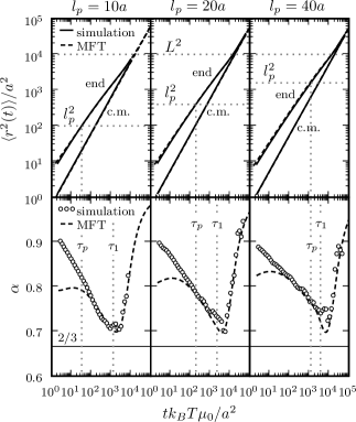
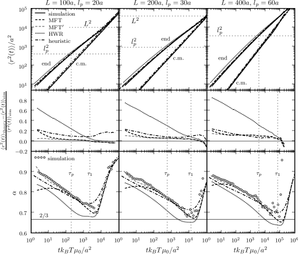
Figure 3: The top panels show simulation and MFT results for the end-monomer and center-of-mass MSD r2(t)/a2delimited-⟨⟩superscript𝑟2𝑡superscript𝑎2\langle r^{2}(t)\rangle/a^{2} for chains of length L=100a𝐿100𝑎L=100a and persistence lengths lp=10asubscript𝑙𝑝10𝑎l_{p}=10a, 20a20𝑎20a, and 40a40𝑎40a (a=𝑎absenta= monomer radius). The bottom panels show the local slope α=dlogr2(t)/dlogt𝛼𝑑superscript𝑟2𝑡𝑑𝑡\alpha=d\log\langle r^{2}(t)\rangle/d\log t for the end-monomer MSD, with a horizontal line at 2/3232/3 marking the Zimm theory prediction. Two times are indicated by dotted vertical lines: τpsubscript𝜏𝑝\tau_{p}, the time at which the end-monomer r2(τp)=lp2delimited-⟨⟩superscript𝑟2subscript𝜏𝑝superscriptsubscript𝑙𝑝2\langle r^{2}(\tau_{p})\rangle=l_{p}^{2}; and τ1subscript𝜏1\tau_{1}, the longest relaxation time of the polymer, as determined from the numerical simulations.
Refer to caption
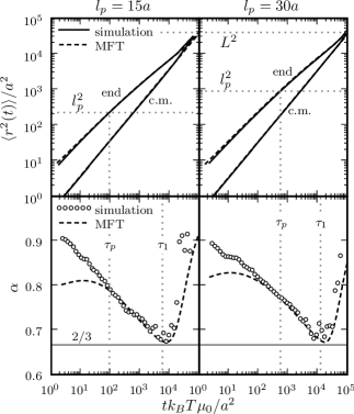
Figure 4: Same as in Fig. 3, but for chains of length L=200a𝐿200𝑎L=200a and persistence lengths lp=15asubscript𝑙𝑝15𝑎l_{p}=15a and 30a30𝑎30a.
Refer to caption
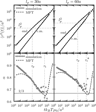
Figure 5: Same as in Fig. 3, but for chains of length L=400a𝐿400𝑎L=400a and persistence lengths lp=30asubscript𝑙𝑝30𝑎l_{p}=30a and 60a60𝑎60a.

The Brownian dynamics simulation and MFT results for the end-monomer and center-of-mass MSD are shown in Figs. 3-5 for chain lengths of L=100a𝐿100𝑎L=100a, 200a200𝑎200a, and 400a400𝑎400a respectively, at various persistence lengths lpsubscript𝑙𝑝l_{p}. We also show in the bottom panels of each figure the effective local exponent α(t)=dlogr2(t)/dlogt𝛼𝑡𝑑superscript𝑟2𝑡𝑑𝑡\alpha(t)=d\log\langle r^{2}(t)\rangle/d\log t of the end-monomer MSD curve.

We find in both the simulation and MFT results that α(t)𝛼𝑡\alpha(t) passes through a minimum in the intermediate time range where lp2<r2(t)<ree2(L)superscriptsubscript𝑙𝑝2delimited-⟨⟩superscript𝑟2𝑡subscriptsuperscript𝑟2ee𝐿l_{p}^{2}<\langle r^{2}(t)\rangle<r^{2}_{\text{ee}}(L). The location of this minimum is on the order of τ1subscript𝜏1\tau_{1}, the longest relaxation time of the polymer. For tτ1much-greater-than𝑡subscript𝜏1t\gg\tau_{1}, as the end-monomer curve approaches the center-of-mass MSD, rc.m.2(t)=6Dtdelimited-⟨⟩subscriptsuperscript𝑟2c.m.𝑡6𝐷𝑡\langle r^{2}_{\text{c.m.}}(t)\rangle=6Dt, the local slope α(t)𝛼𝑡\alpha(t) tends toward the limiting value of 1. On the other hand, for t<τp𝑡subscript𝜏𝑝t<\tau_{p}, where r2(t)<lp2delimited-⟨⟩superscript𝑟2𝑡superscriptsubscript𝑙𝑝2\langle r^{2}(t)\rangle<l_{p}^{2}, the stiffness of the polymer dominates, and α(t)𝛼𝑡\alpha(t) varies in the range 0.80.9absent0.80.9\approx 0.8-0.9. We will discuss both the intermediate and the short-time regimes in more detail below.
Refer to caption
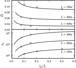
Figure 6: Diffusion constant D~=D/(kBTμ0)~𝐷𝐷subscript𝑘𝐵𝑇subscript𝜇0\tilde{D}=D/(k_{B}T\mu_{0}) (top) and longest relaxation time τ~1=τ1kBTμ0/a2subscript~𝜏1subscript𝜏1subscript𝑘𝐵𝑇subscript𝜇0superscript𝑎2\tilde{\tau}_{1}=\tau_{1}k_{B}T\mu_{0}/a^{2} (bottom) as a function of lp/Lsubscript𝑙𝑝𝐿l_{p}/L for three different chain lengths L𝐿L. The squares are Brownian dynamics simulation results, while the solid curves are calculated from MFT.
Refer to caption
Figure 7: Comparison of the simulation results for three semiflexible chains with several analytical approaches: the heuristic scaling argument described in Sec. 2, the MFT described in Sec. 4, and the MFT, HWR [9] models described in Sec. 5. The top panels show the end-monomer and center-of-mass MSD r2(t)delimited-⟨⟩superscript𝑟2𝑡\langle r^{2}(t)\rangle; the middle panels show the relative difference between the various theoretical results for the end-monomer MSD and the simulation data; the bottom panels show the local slope α=dlogr2(t)/dlogt𝛼𝑑superscript𝑟2𝑡𝑑𝑡\alpha=d\log\langle r^{2}(t)\rangle/d\log t for the end-monomer MSD. Two times are indicated by dotted vertical lines: τpsubscript𝜏𝑝\tau_{p}, the time at which the end-monomer r2(τp)=lp2delimited-⟨⟩superscript𝑟2subscript𝜏𝑝superscriptsubscript𝑙𝑝2\langle r^{2}(\tau_{p})\rangle=l_{p}^{2}; and τ1subscript𝜏1\tau_{1}, the longest relaxation time of the polymer. The τ1subscript𝜏1\tau_{1} and τpsubscript𝜏𝑝\tau_{p} values shown are from the numerical simulations.

There is very good agreement between MFT end-monomer MSD predictions and simulation results in time regimes where simulation results have sufficiently converged to make a comparison. (For r2(t)delimited-⟨⟩superscript𝑟2𝑡\langle r^{2}(t)\rangle this comparison is possible for nearly the whole simulation time range; for α(t)𝛼𝑡\alpha(t) the numerical uncertainty at the largest times becomes significant, and is on the order of the scatter in the plotted data points.) Additionally, dynamical parameters like the diffusion constant D𝐷D and relaxation time τ1subscript𝜏1\tau_{1} determined from the simulation data compare favorably with their MFT values, as shown in Fig. 6. The values of D𝐷D were obtained from the simulations by fitting the center-of-mass MSD data to the straight-line form rc.m.2(t)=6Dtdelimited-⟨⟩subscriptsuperscript𝑟2c.m.𝑡6𝐷𝑡\langle r^{2}_{\text{c.m.}}(t)\rangle=6Dt. To extract τ1subscript𝜏1\tau_{1}, the autocorrelation function of the end-to-end vector was calculated, Cee(t)=𝐫ee(t)𝐫ee(0)subscript𝐶ee𝑡delimited-⟨⟩subscript𝐫ee𝑡subscript𝐫ee0C_{\text{ee}}(t)=\langle\mathbf{r}_{\text{ee}}(t)\cdot\mathbf{r}_{\text{ee}}(0)\rangle, where 𝐫ee(t)=𝐫M(t)𝐫1(t)subscript𝐫ee𝑡subscript𝐫𝑀𝑡subscript𝐫1𝑡\mathbf{r}_{\text{ee}}(t)=\mathbf{r}_{M}(t)-\mathbf{r}_{1}(t). For sufficiently large t𝑡t, this function takes the form of a simple exponential decay, Cee(t)exp(t/τ1)similar-tosubscript𝐶ee𝑡𝑡subscript𝜏1C_{\text{ee}}(t)\sim\exp(-t/\tau_{1}), from which τ1subscript𝜏1\tau_{1} can be estimated. For both D𝐷D and τ1subscript𝜏1\tau_{1}, only data points for which convergence was achieved were included in the fitting (the criterion for convergence was that the local slope dlog𝐫c.m.2(t)/dlogt1𝑑subscriptsuperscript𝐫2c.m.𝑡𝑑𝑡1d\log\langle\mathbf{r}^{2}_{\text{c.m.}}(t)\rangle/d\log t\approx 1.)

The main discrepancies between the two approaches are in the local slopes of the MSD curves at the shortest times, t102a2/(kBTμ0)less-than-or-similar-to𝑡superscript102superscript𝑎2subscript𝑘𝐵𝑇subscript𝜇0t\lesssim 10^{2}\>a^{2}/(k_{B}T\mu_{0}). This can be explained by the fact that the small-scale motions at short times are particularly sensitive to the discrete nature of the polymer chain and the more strongly fixed monomer-monomer separation in the simulation, thus giving rise to differences with the continuum mean-field approximation. In fact we can make the MFT mimic the simulation more closely if we exclude the contributions of a fraction of the highest modes in the sum of Eq. (37), by changing the upper limit from N1𝑁1N-1 to N1superscript𝑁1N^{\prime}-1, where N=cL/4asuperscript𝑁𝑐𝐿4𝑎N^{\prime}=cL/4a, 0<c<10𝑐10<c<1. A value of c1/2𝑐12c\approx 1/2 gives the closest approximation to the simulation MSD and α(t)𝛼𝑡\alpha(t) curves, irrespective of L𝐿L and lpsubscript𝑙𝑝l_{p}. This roughly corresponds to excluding modes where the distance between nodes is shorter than four monomer diameters. The results are shown in Fig. 7 for three different chains, with the modified MFT labeled as MFT. The long-time behavior is unaffected by removing the highest modes, but at short times the MFT α(t)𝛼𝑡\alpha(t) curves fit the simulation data much more closely. We rationalize this as being due to an effective cutoff of fluctuations at small wavelengths due to the spring stiffness in the simulation, which is not represented well by the Gaussian MFT elastic energy in Eq. (17).
Refer to caption
Figure 8: Results of the MFT for various semiflexible chains. (a) The end-monomer MSD effective exponent α=dlogr2(t)/dlogt𝛼𝑑superscript𝑟2𝑡𝑑𝑡\alpha=d\log\langle r^{2}(t)\rangle/d\log t versus t/τ1𝑡subscript𝜏1t/\tau_{1} for polymers of diameter 2a2𝑎2a, contour length L=12000a𝐿12000𝑎L=12000a, and various persistence lengths lp=50a3000asubscript𝑙𝑝50𝑎3000𝑎l_{p}=50a-3000a. The dot along each α(t)𝛼𝑡\alpha(t) curve marks α(τp)𝛼subscript𝜏𝑝\alpha(\tau_{p}). The time τpsubscript𝜏𝑝\tau_{p} is where r2(τp)=lp2delimited-⟨⟩superscript𝑟2subscript𝜏𝑝superscriptsubscript𝑙𝑝2\langle r^{2}(\tau_{p})\rangle=l_{p}^{2}, and τ1subscript𝜏1\tau_{1} is the longest relaxation time of the polymer. (b) The minimum value of α𝛼\alpha over all t𝑡t versus lp/Lsubscript𝑙𝑝𝐿l_{p}/L for several chain lengths L=100a12000a𝐿100𝑎12000𝑎L=100a-12000a. (c) The minimum value of α𝛼\alpha over all t𝑡t versus L/lp𝐿subscript𝑙𝑝L/l_{p} for several lp=50a1800asubscript𝑙𝑝50𝑎1800𝑎l_{p}=50a-1800a. (d) The circles show the minimum value of α𝛼\alpha in each of the curves in panel (b), plotted as a function of 1/log(L/a)1𝐿𝑎1/\log(L/a). Superimposed is a straight-line fit to the data points. The squares, with the dashed straight-line fit, are the corresponding results of the heuristic scaling argument, taken from Fig. 1(d).
Refer to caption
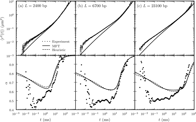
Figure 9: Comparison of the MFT and heuristic scaling results to experimental MSD data taken from Ref. 2 for three lengths of double-stranded DNA: (a) 2400 bp; (b) 6700 bp; (c) 23100 bp. The dimensional parameters in the theories are fixed at: a=1𝑎1a=1 nm, rise per bp =0.34absent0.34=0.34 nm, lp=50subscript𝑙𝑝50l_{p}=50 nm, T=293𝑇293T=293K, viscosity of water at 293K = 1 mPa s. The top panels show the end-monomer MSD r2(t)delimited-⟨⟩superscript𝑟2𝑡\langle r^{2}(t)\rangle, and the bottom panels show the corresponding effective local exponent α=dlogr2(t)/dlogt𝛼𝑑superscript𝑟2𝑡𝑑𝑡\alpha=d\log\langle r^{2}(t)\rangle/d\log t.

In Fig. 7 we also show the MSD and α(t)𝛼𝑡\alpha(t) curves calculated using the HWR model. This model follows the same basic approach as in Sec. 4, with two additional approximations: (i) only the diagonal elements Hnnsubscript𝐻𝑛𝑛H_{nn} of Eq. (34) are used; (ii) for n>1𝑛1n>1, the Hnnsubscript𝐻𝑛𝑛H_{nn} are evaluated approximately as [9]

Hnn26πμ0aLdL𝑑sLsσ(s)exp(3d22σ(s))cosαns.subscript𝐻𝑛𝑛26𝜋subscript𝜇0𝑎𝐿superscriptsubscript𝑑𝐿differential-d𝑠𝐿𝑠𝜎𝑠3superscript𝑑22𝜎𝑠subscript𝛼𝑛𝑠H_{nn}\approx 2\sqrt{\frac{6}{\pi}}\frac{\mu_{0}a}{L}\int_{d}^{L}ds\,\frac{L-s}{\sqrt{\sigma(s)}}\exp\left(-\frac{3d^{2}}{2\sigma(s)}\right)\cos\alpha_{n}s\,. (38)

The net effect of these approximations is negligible only for tτ1greater-than-or-equivalent-to𝑡subscript𝜏1t\gtrsim\tau_{1}, where the HWR and MFT results overlap. For t<τ1𝑡subscript𝜏1t<\tau_{1} there are significant differences with respect to the simulations. Here the HWR model overestimates the end-monomer MSD and underestimates α(t)𝛼𝑡\alpha(t). The discrepancy is only slightly reduced by avoiding the approximation of Eq. (38); the main weakness of the HWR model is that the off-diagonal matrix elements Hnmsubscript𝐻𝑛𝑚H_{nm} are not included in the calculation. Taking these into account, as the MFT results demonstrate, gives a much more accurate description of the simulation data at short and intermediate times. Despite these differences, the sub-Zimm scaling regime exists in the HWR model, and the deviation below 2/3 is even larger than in the MFT. (The sub-Zimm scaling is also implicitly evident in related quantities calculated from the HWR approach, like the fluorescence correlation function studied in Ref. 3.)

For comparison, Fig. 7 also shows the r2(t)delimited-⟨⟩superscript𝑟2𝑡\langle r^{2}(t)\rangle and α(t)𝛼𝑡\alpha(t) curves calculated from the heuristic scaling argument of Sec. 2. Despite its simplicity, it is able to capture the trends of the simulation and MFT data quite well, though for shorter chain lengths it gives a shallower dip in α𝛼\alpha within the intermediate regime.

Given the success of the MFT at reproducing the simulation results, it is interesting to see what the theory predicts for longer chain lengths where Brownian hydrodynamics simulations become impractical. Fig. 8(a) shows α(t)𝛼𝑡\alpha(t) curves for L=12000a𝐿12000𝑎L=12000a, lp=50a3000asubscript𝑙𝑝50𝑎3000𝑎l_{p}=50a-3000a, with the point α(τp)𝛼subscript𝜏𝑝\alpha(\tau_{p}) on each curve marked by a dot. As in the shorter chains, there is a broad dip in α(t)𝛼𝑡\alpha(t) between τpsubscript𝜏𝑝\tau_{p} and τ1subscript𝜏1\tau_{1}, but the minimum of α(t)𝛼𝑡\alpha(t) has been shifted to below 2/3232/3. In fact the dependence of this minimum on L𝐿L and lpsubscript𝑙𝑝l_{p}, illustrated in Fig. 8(b-d), is qualitatively the same as that derived from the heuristic scaling argument in Fig. 1(b-d): there is a general trend of mintαsubscript𝑡𝛼\min_{t}\alpha decreasing with L𝐿L, and in particular the smallest value possible at a given L𝐿L, minlpmintαsubscriptsubscript𝑙𝑝subscript𝑡𝛼\min_{l_{p}}\min_{t}\alpha, has a nearly linear dependence on 1/log(L/a)1𝐿𝑎1/\log(L/a) (the heuristic result from Fig. 1(d) is also drawn for reference).

At lp=50asubscript𝑙𝑝50𝑎l_{p}=50a, corresponding to the persistence length of DNA, mintαsubscript𝑡𝛼\min_{t}\alpha ranges from 0.698 at L=100a𝐿100𝑎L=100a to 0.617 at L=12000a𝐿12000𝑎L=12000a. Within this range we can make a detailed comparison for three particular chain lengths where experimental MSD data for double-stranded DNA is available from Ref. 2: L=816a𝐿816𝑎L=816a, 2278a2278𝑎2278a, and 7854a7854𝑎7854a, or equivalently 2400 bp, 6700 bp, and 23100 bp (using a=1𝑎1a=1 nm, and a rise per base pair of 0.34 nm). The experimental end-monomer MSD for these three cases is shown in the top panels of Fig. 9. The bottom panels show the local slope α(t)𝛼𝑡\alpha(t), which can be estimated at each t𝑡t by fitting straight lines to the log-log plot of MSD data points with times tisubscript𝑡𝑖t_{i} within a small range around t𝑡t, defined by the condition |log10ti/t|<0.15subscript10subscript𝑡𝑖𝑡0.15|\log_{10}t_{i}/t|<0.15. Together with the experimental results for the MSD and α(t)𝛼𝑡\alpha(t) are the curves predicted by the MFT and heuristic scaling argument. Besides the length scale parameters mentioned above, the other dimensional variables in the system are set at the following values (taken from the literature and the experimental conditions): lp=50subscript𝑙𝑝50l_{p}=50 nm, T=293𝑇293T=293K, viscosity of water at 293K = 1 mPa s. At longer times (>10absent10>10 ms) there is quite good agreement between both theories and experimental data, particularly notable since there is no fitting parameter involved in the MFT. The discrepancies arise in the short and intermediate time regime, where the experimental MSD is consistently higher than the theoretical one, the difference increasing to roughly a factor of 23232-3 at the shortest times measured. The discrepancy in the MSD is on the order of 0.0010.010.0010.010.001-0.01 μm2𝜇superscriptm2\mu\text{m}^{2}, corresponding to length scales roughly 301003010030-100 nm. Experimental data seems to indicate faster displacement of the end monomer at very short times followed by slower increase of the MSD at intermediate times compared to the theoretical predictions.

The effect of the higher experimental MSD is to push the local slope down relative to the theoretical value. Thus the intermediate dynamical regime, in the range 0.01100.01100.01-10 ms, is characterized by a broad region with α(t)𝛼𝑡\alpha(t) close to 0.5, in contrast to the MFT results where mintαsubscript𝑡𝛼\min_{t}\alpha is between 0.633 for L=2400𝐿2400L=2400 bp and 0.617 for L=23100𝐿23100L=23100 bp. Though there are large uncertainties in the experimental data for t<0.01𝑡0.01t<0.01 ms (on average 50% for L=2400𝐿2400L=2400 bp, going down to 10% for L=23100𝐿23100L=23100 bp), the rough trend in the local slope appears to show a rapid increase in α(t)𝛼𝑡\alpha(t) as t𝑡t is decreased. This rapid crossover again contrasts with the MFT curve, where the increase in the local slope is more gradual. The heuristic scaling results support the MFT: with the crossover exponents and fitting constants set at the values shown below Eq. (6), the heuristic r2(t)delimited-⟨⟩superscript𝑟2𝑡\langle r^{2}(t)\rangle almost perfectly overlaps with the MFT curve in all three cases, and the local slopes are consequently also very similar. Independently, we also checked if it was possible to find an alternative set of fitting parameters which would make the heuristic r2(t)delimited-⟨⟩superscript𝑟2𝑡\langle r^{2}(t)\rangle agree with the experimental data, but we were unable to obtain a reasonable fit.

Although the existence of an intermediate regime with sub-Zimm scaling is found in both experiment and theory, the quantitative discrepancy of the scaling behavior points to a gap between the experimental system and the theoretical approaches. Possibly, a semiflexible polymer model based on a worm-like chain is sufficient only for describing the large-scale motions of the DNA. There may be some missing elements in the theory (for example an additional degree of freedom present in DNA, like torsional dynamics) that lead to faster motion at shorter scales. On the other hand, there is also the possibility that limitations in the setup and analysis of FCS measurements could contribute to the discrepancy. Deviations from the assumed Gaussian profile of the confocal detection volume and uncertainties in the diffusion coefficient of the rhodamine molecule used to calibrate the shape of this volume have been shown by alternative methods like two-focus FCS to lead to substantial systematic errors in the single-focus setup [28]. The uncertainties in the FCS analysis are highlighted by the differing results produced by independent studies of similar double-stranded DNA systems: one yielding a substantial sub-Zimm regime [2], with local exponents near the Rouse limit, and others giving a smaller deviation below the Zimm value over shorter time ranges [5, 3], as fitted by the HWR model. Regardless of these issues, there is one aspect in which both the experimental and theoretical approaches agree: an intermediate dynamical regime is present in the end-monomer MSD results, and this regime shows sub-Zimm scaling for long enough chains.

6 Discussion
Refer to caption
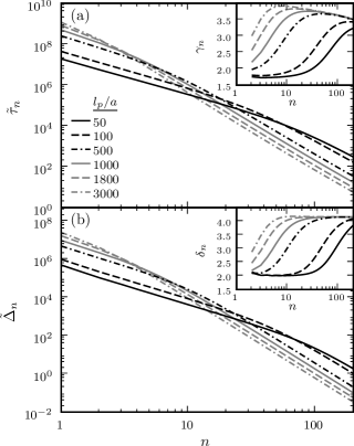
Figure 10: The values of (a) τ~n=τnkBTμ0/a2subscript~𝜏𝑛subscript𝜏𝑛subscript𝑘𝐵𝑇subscript𝜇0superscript𝑎2\tilde{\tau}_{n}=\tau_{n}k_{B}T\mu_{0}/a^{2}, (b) Δ~n=Δn/a2subscript~Δ𝑛subscriptΔ𝑛superscript𝑎2\tilde{\Delta}_{n}=\Delta_{n}/a^{2} as a function of mode number n𝑛n for a semiflexible polymer of length L=12000a𝐿12000𝑎L=12000a with various lp=50a3000asubscript𝑙𝑝50𝑎3000𝑎l_{p}=50a-3000a, calculated using MFT. The parameters ΔnsubscriptΔ𝑛\Delta_{n} and relaxation times τnsubscript𝜏𝑛\tau_{n} determine the subdiffusive behavior of the end-monomer MSD through Eq. (37). The insets show the effective local exponents describing the scaling of τnsubscript𝜏𝑛\tau_{n} and ΔnsubscriptΔ𝑛\Delta_{n} with n𝑛n: γn=dlogτn/dlognsubscript𝛾𝑛𝑑subscript𝜏𝑛𝑑𝑛\gamma_{n}=-d\log\tau_{n}/d\log n, δn=dlogΔn/dlognsubscript𝛿𝑛𝑑subscriptΔ𝑛𝑑𝑛\delta_{n}=-d\log\Delta_{n}/d\log n.

To understand the intermediate dynamical regime in more detail, and to see where the deviations from the Zimm model arise, let us analyze the behavior of Eq. (37), whose general form is shared by any theory that expresses the end-monomer MSD in terms of contributions from normal modes. Both τnsubscript𝜏𝑛\tau_{n} and ΔnsubscriptΔ𝑛\Delta_{n} decrease approximately as power laws in n𝑛n, and we can describe this decrease through effective local exponents γnsubscript𝛾𝑛\gamma_{n}, δn>1subscript𝛿𝑛1\delta_{n}>1:

γn=dlogτndlogn,δn=dlogΔndlogn.formulae-sequencesubscript𝛾𝑛𝑑subscript𝜏𝑛𝑑𝑛subscript𝛿𝑛𝑑subscriptΔ𝑛𝑑𝑛\gamma_{n}=-\frac{d\log\tau_{n}}{d\log n},\qquad\delta_{n}=-\frac{d\log\Delta_{n}}{d\log n}\,. (39)

Several examples of τnsubscript𝜏𝑛\tau_{n} and ΔnsubscriptΔ𝑛\Delta_{n} are plotted in Fig. 10 for L=12000a𝐿12000𝑎L=12000a and lp=50a3000asubscript𝑙𝑝50𝑎3000𝑎l_{p}=50a-3000a. The variation of γnsubscript𝛾𝑛\gamma_{n} and δnsubscript𝛿𝑛\delta_{n} with n𝑛n is shown in the insets. The behavior of the MSD slope α(t)𝛼𝑡\alpha(t) can be directly related to these local exponents. Let us assume that within some time range τn2tτn1much-less-thansubscript𝜏subscript𝑛2𝑡much-less-thansubscript𝜏subscript𝑛1\tau_{n_{2}}\ll t\ll\tau_{n_{1}}, n2n1much-greater-thansubscript𝑛2subscript𝑛1n_{2}\gg n_{1}, the associated normal mode exponents are approximately constant: γnγsubscript𝛾𝑛𝛾\gamma_{n}\approx\gamma, δnδsubscript𝛿𝑛𝛿\delta_{n}\approx\delta for n1<n<n2subscript𝑛1𝑛subscript𝑛2n_{1}<n<n_{2}. Then the dominant contribution to the subdiffusive behavior at times t𝑡t within this range is given by:

r2(t)n=n1n2Δn(1et/τn)Δn1n1δn1𝑑nnδ(1etnγ/τn1n1γ)=Δn1n1(1δ1+1γE1+δ1γ(t/τn1)).delimited-⟨⟩superscript𝑟2𝑡superscriptsubscript𝑛subscript𝑛1subscript𝑛2subscriptΔ𝑛1superscript𝑒𝑡subscript𝜏𝑛subscriptΔsubscript𝑛1superscriptsubscript𝑛1𝛿superscriptsubscriptsubscript𝑛1differential-d𝑛superscript𝑛𝛿1superscript𝑒𝑡superscript𝑛𝛾subscript𝜏subscript𝑛1superscriptsubscript𝑛1𝛾subscriptΔsubscript𝑛1subscript𝑛11𝛿11𝛾subscript𝐸1𝛿1𝛾𝑡subscript𝜏subscript𝑛1\begin{split}\langle r^{2}(t)\rangle&\approx\sum_{n=n_{1}}^{n_{2}}\Delta_{n}(1-e^{-t/\tau_{n}})\\ &\approx\Delta_{n_{1}}n_{1}^{\delta}\int_{n_{1}}^{\infty}dn\>n^{-\delta}(1-e^{-tn^{\gamma}/\tau_{n_{1}}n_{1}^{\gamma}})\\ &=\Delta_{n_{1}}n_{1}\left(\frac{1}{\delta-1}+\frac{1}{\gamma}E_{1+\frac{\delta-1}{\gamma}}(t/\tau_{n_{1}})\right).\end{split} (40)

In the second line we extended the upper limit of the integration from n2subscript𝑛2n_{2} to \infty using the fact that tτn2much-greater-than𝑡subscript𝜏subscript𝑛2t\gg\tau_{n_{2}}, n2n1much-greater-thansubscript𝑛2subscript𝑛1n_{2}\gg n_{1}, and in the third line Eν(x)subscript𝐸𝜈𝑥E_{\nu}(x) denotes the exponential integral function, Eν(z)1𝑑texp(zt)/tνsubscript𝐸𝜈𝑧superscriptsubscript1differential-d𝑡𝑧𝑡superscript𝑡𝜈E_{\nu}(z)\equiv\int_{1}^{\infty}dt\,\exp(-zt)/t^{\nu}. For tτn1much-less-than𝑡subscript𝜏subscript𝑛1t\ll\tau_{n_{1}}, Eq. (40) can be expanded to the leading order as

r2(t)Δn1n1δ1Γ(1δ+γγ)(tτn1)δ1γ.delimited-⟨⟩superscript𝑟2𝑡subscriptΔsubscript𝑛1subscript𝑛1𝛿1Γ1𝛿𝛾𝛾superscript𝑡subscript𝜏subscript𝑛1𝛿1𝛾\langle r^{2}(t)\rangle\approx\frac{\Delta_{n_{1}}n_{1}}{\delta-1}\Gamma\left(\frac{1-\delta+\gamma}{\gamma}\right)\left(\frac{t}{\tau_{n_{1}}}\right)^{\frac{\delta-1}{\gamma}}\,. (41)

This implies that for τn2tτn1much-less-thansubscript𝜏subscript𝑛2𝑡much-less-thansubscript𝜏subscript𝑛1\tau_{n_{2}}\ll t\ll\tau_{n_{1}} the local slope is given by α(t)(δ1)/γ𝛼𝑡𝛿1𝛾\alpha(t)\approx(\delta-1)/\gamma. As can be seen in the insets of Fig. 10, there are two distinct regimes for γnsubscript𝛾𝑛\gamma_{n} and δnsubscript𝛿𝑛\delta_{n}: one for modes nL/lpmuch-less-than𝑛𝐿subscript𝑙𝑝n\ll L/l_{p}, corresponding to length scales greater than lpsubscript𝑙𝑝l_{p}, and another for modes nL/lpmuch-greater-than𝑛𝐿subscript𝑙𝑝n\gg L/l_{p}, corresponding to length scales smaller than lpsubscript𝑙𝑝l_{p}. A continuous crossover occurs from one regime to the other for nO(L/lp)similar-to𝑛O𝐿subscript𝑙𝑝n\sim\text{O}(L/l_{p}). These two regimes in turn lead to differing behaviors for α(t)𝛼𝑡\alpha(t). We will consider each regime separately, focusing on earlier predictions for each case and how they compare to the present results.

Modes with nL/lpmuch-less-than𝑛𝐿subscript𝑙𝑝n\ll L/l_{p} correspond to internal polymer dynamics on length scales between lpsubscript𝑙𝑝l_{p} and L𝐿L, and this is precisely the intermediate dynamical regime that we have mentioned earlier. In the simplest analysis, ignoring hydrodynamical effects, these modes should be described by the Rouse model, particularly in the flexible limit of small n𝑛n where the length scales are much greater than lpsubscript𝑙𝑝l_{p}. The Rouse theory yields the following expressions for τnsubscript𝜏𝑛\tau_{n} and ΔnsubscriptΔ𝑛\Delta_{n} [7],

τnRouse=L2b212π2kBTμ0a2n2,ΔnRouse=2Lb2aπ2n2.formulae-sequencesubscriptsuperscript𝜏Rouse𝑛superscript𝐿2superscript𝑏212superscript𝜋2subscript𝑘𝐵𝑇subscript𝜇0superscript𝑎2superscript𝑛2subscriptsuperscriptΔRouse𝑛2𝐿superscript𝑏2𝑎superscript𝜋2superscript𝑛2\tau^{\text{Rouse}}_{n}=\frac{L^{2}b^{2}}{12\pi^{2}k_{B}T\mu_{0}a^{2}}n^{-2},\quad\Delta^{\text{Rouse}}_{n}=\frac{2Lb^{2}}{a\pi^{2}}n^{-2}\,. (42)

where b𝑏b is the Kuhn length, b=ree2(L)/M𝑏subscriptsuperscript𝑟2ee𝐿𝑀b=\sqrt{r^{2}_{\text{ee}}(L)/M}. The local exponents in the Rouse model are constants: δn=2subscript𝛿𝑛2\delta_{n}=2 and γn=2subscript𝛾𝑛2\gamma_{n}=2. Using Eq. (41), we find the following asymptotic behavior for the end-monomer MSD:

r2(t)Δ1RouseΓ(1/2)(t/τ1Rouse)1/2=(48b2kBTμ0π)1/2t1/2.delimited-⟨⟩superscript𝑟2𝑡subscriptsuperscriptΔRouse1Γ12superscript𝑡superscriptsubscript𝜏1Rouse12superscript48superscript𝑏2subscript𝑘𝐵𝑇subscript𝜇0𝜋12superscript𝑡12\begin{split}\langle r^{2}(t)\rangle&\approx\Delta^{\text{Rouse}}_{1}\Gamma(1/2)(t/\tau_{1}^{\text{Rouse}})^{1/2}\\ &=\left(\frac{48b^{2}k_{B}T\mu_{0}}{\pi}\right)^{1/2}t^{1/2}\,.\end{split} (43)

This is the origin of the Rouse scaling result α(t)=1/2𝛼𝑡12\alpha(t)=1/2. In the presence of hydrodynamic interactions, the Zimm model is expected to hold, with Eq. (42) modified as: [7]

τnZimm=b3(L/πa)3/2126kBTμ0an3/2,ΔnZimm=ΔnRouse.formulae-sequencesubscriptsuperscript𝜏Zimm𝑛superscript𝑏3superscript𝐿𝜋𝑎32126subscript𝑘𝐵𝑇subscript𝜇0𝑎superscript𝑛32subscriptsuperscriptΔZimm𝑛subscriptsuperscriptΔRouse𝑛\tau^{\text{Zimm}}_{n}=\frac{b^{3}(L/\pi a)^{3/2}}{12\sqrt{6}k_{B}T\mu_{0}a}n^{-3/2},\quad\Delta^{\text{Zimm}}_{n}=\Delta^{\text{Rouse}}_{n}\,. (44)

Here the local exponent γnsubscript𝛾𝑛\gamma_{n} is 3/2, and thus the asymptotic behavior of the MSD becomes:

r2(t)12Γ(1/3)(2akBTμ0)2/3πt2/3,delimited-⟨⟩superscript𝑟2𝑡12Γ13superscript2𝑎subscript𝑘𝐵𝑇subscript𝜇023𝜋superscript𝑡23\begin{split}\langle r^{2}(t)\rangle\approx\frac{12\Gamma(1/3)(2ak_{B}T\mu_{0})^{2/3}}{\pi}t^{2/3}\,,\end{split} (45)

leading to the Zimm scaling α(t)=2/3𝛼𝑡23\alpha(t)=2/3.

The MFT calculations, however, give a different picture, deviating from the Zimm result. Consider the chain in Fig. 10 closest to the flexible limit: L=12000a𝐿12000𝑎L=12000a, lp=50asubscript𝑙𝑝50𝑎l_{p}=50a. The exponents γnsubscript𝛾𝑛\gamma_{n} and δnsubscript𝛿𝑛\delta_{n} are approximately constant for n10less-than-or-similar-to𝑛10n\lesssim 10, but are shifted from the Zimm values: γ1.74𝛾1.74\gamma\approx 1.74, δ2.04𝛿2.04\delta\approx 2.04 averaged over n=110𝑛110n=1-10, giving α=(δ1)/γ0.60𝛼𝛿1𝛾0.60\alpha=(\delta-1)/\gamma\approx 0.60. Indeed in the corresponding local slope curve plotted in Fig. 8(a) the α(t)𝛼𝑡\alpha(t) value is nearly constant over the time scales associated with these modes (t/τ10.0181𝑡subscript𝜏10.0181t/\tau_{1}\approx 0.018-1), reaching a minimum of 0.617. It is these shifts in γnsubscript𝛾𝑛\gamma_{n} and δnsubscript𝛿𝑛\delta_{n} from the Zimm theory predictions that lead to an intermediate dynamical regime for longer chains where α(t)<2/3𝛼𝑡23\alpha(t)<2/3.

To get an analytical estimate for these shifts within the framework of the MFT theory, one can approximately evaluate the integrals for the interaction matrix elements Hnmsubscript𝐻𝑛𝑚H_{nm} in Eq. (34), and account for the effects of the off-diagonal elements using perturbation theory. The details of the approximation can be found in Appendix B. For nL/lpmuch-less-than𝑛𝐿subscript𝑙𝑝n\ll L/l_{p} the results are:

γn3p1(n)+5.07p2(n)nlpLK(6a2lp2)2p3(n)+2.89p4(n)nlpLK(6a2lp2),δn2p5(n)+0.0393p6(n)lpnLK(6a2lp2)p7(n)+0.0157p8(n)lpnLK(6a2lp2),\begin{split}\gamma_{n}&\approx\frac{3p_{1}(n)+5.07p_{2}(n)\sqrt{\frac{nl_{p}}{L}}K\left(\frac{6a^{2}}{l_{p}^{2}}\right)}{2p_{3}(n)+2.89p_{4}(n)\sqrt{\frac{nl_{p}}{L}}K\left(\frac{6a^{2}}{l_{p}^{2}}\right)},\quad\delta_{n}\approx\frac{2p_{5}(n)+0.0393p_{6}(n)\sqrt{\frac{l_{p}}{nL}}K\left(\frac{6a^{2}}{l_{p}^{2}}\right)}{p_{7}(n)+0.0157p_{8}(n)\sqrt{\frac{l_{p}}{nL}}K\left(\frac{6a^{2}}{l_{p}^{2}}\right)},\\ \end{split} (46)

where K(x)6π(E1(x)E1(3/2))43π+2𝐾𝑥6𝜋subscript𝐸1𝑥subscript𝐸13243𝜋2K(x)\equiv\sqrt{\frac{6}{\pi}}\left(E_{1}(x)-E_{1}(3/2)\right)-4\sqrt{\frac{3}{\pi}}+2, and p1(n),,p8(n)subscript𝑝1𝑛subscript𝑝8𝑛p_{1}(n),\ldots,p_{8}(n) are polynomials in n𝑛n of the form pi(n)=1+ai/n+bi/n2+subscript𝑝𝑖𝑛1subscript𝑎𝑖𝑛subscript𝑏𝑖superscript𝑛2p_{i}(n)=1+a_{i}/n+b_{i}/n^{2}+\cdots, with coefficients aisubscript𝑎𝑖a_{i} and bisubscript𝑏𝑖b_{i} given in Table 1 of Appendix B. For Lamuch-greater-than𝐿𝑎L\gg a and lpsubscript𝑙𝑝l_{p} approaching the flexible limit, lp2asubscript𝑙𝑝2𝑎l_{p}\to 2a, the first terms in the numerators and denominators of the γnsubscript𝛾𝑛\gamma_{n} and δnsubscript𝛿𝑛\delta_{n} expressions dominate, and thus there is a range of modes 1nL/lpmuch-less-than1𝑛much-less-than𝐿subscript𝑙𝑝1\ll n\ll L/l_{p} where γn3/2subscript𝛾𝑛32\gamma_{n}\approx 3/2 and δn2subscript𝛿𝑛2\delta_{n}\approx 2, in agreement with the expected Zimm scaling for a flexible chain. However, for a semiflexible chain where lpamuch-greater-thansubscript𝑙𝑝𝑎l_{p}\gg a, corrections to the Zimm values become more important. Using the fact that E1(z)logzsubscript𝐸1𝑧𝑧E_{1}(z)\approx-\log z as z0𝑧0z\to 0, the K(6a2/lp2)𝐾6superscript𝑎2superscriptsubscript𝑙𝑝2K(6a^{2}/l_{p}^{2}) terms in the γnsubscript𝛾𝑛\gamma_{n} expression lead to a positive shift of order (nlp/L)1/2log(lp/a)superscript𝑛subscript𝑙𝑝𝐿12subscript𝑙𝑝𝑎(nl_{p}/L)^{1/2}\log(l_{p}/a). For δnsubscript𝛿𝑛\delta_{n} the shift upward is smaller, of order (lp/nL)1/2log(lp/a)superscriptsubscript𝑙𝑝𝑛𝐿12subscript𝑙𝑝𝑎(l_{p}/nL)^{1/2}\log(l_{p}/a). These corrections due to semiflexibility are evident in the exact numerical results for chains of length L=12000a𝐿12000𝑎L=12000a shown in the insets of Fig. 10, particularly for lp=50asubscript𝑙𝑝50𝑎l_{p}=50a and 100a100𝑎100a where a nL/lpmuch-less-than𝑛𝐿subscript𝑙𝑝n\ll L/l_{p} regime is identifiable. As expected from the analytical approximation, the deviation in γnsubscript𝛾𝑛\gamma_{n} from the Zimm value is more significant than that of δnsubscript𝛿𝑛\delta_{n}. In fact the averages of γnsubscript𝛾𝑛\gamma_{n} and δnsubscript𝛿𝑛\delta_{n} for n=110𝑛110n=1-10 from the approximate expressions in Eq. (46) are 1.68 and 2.06 respectively, comparable to the numerical results 1.74 and 2.04 quoted above.

In the other regime, for modes with nL/lpmuch-greater-than𝑛𝐿subscript𝑙𝑝n\gg L/l_{p}, the oscillations are at length scales smaller than lpsubscript𝑙𝑝l_{p}, where the rigidity of the chain is the dominating factor. For this case it is easiest to consider first the MFT in the absence of hydrodynamic interactions, and then see how the final results are modified when the interactions are included. In the free-draining limit, the interaction matrix Hnm=2aμ0δnmsubscript𝐻𝑛𝑚2𝑎subscript𝜇0subscript𝛿𝑛𝑚H_{nm}=2a\mu_{0}\delta_{nm}, and for large n𝑛n the constants αnsubscript𝛼𝑛\alpha_{n} in Eqs. (31)-(32) are approximately αnnπ/Lsubscript𝛼𝑛𝑛𝜋𝐿\alpha_{n}\approx n\pi/L [9]. With these simplifications we find

τnL43aμ0lpkBTπ4n4,Δn16L3lpπ4n4,formulae-sequencesubscript𝜏𝑛superscript𝐿43𝑎subscript𝜇0subscript𝑙𝑝subscript𝑘𝐵𝑇superscript𝜋4superscript𝑛4subscriptΔ𝑛16superscript𝐿3subscript𝑙𝑝superscript𝜋4superscript𝑛4\tau_{n}\approx\frac{L^{4}}{3a\mu_{0}l_{p}k_{B}T\pi^{4}}n^{-4},\quad\Delta_{n}\approx\frac{16L^{3}}{l_{p}\pi^{4}}n^{-4}\,, (47)

for nL/lpmuch-greater-than𝑛𝐿subscript𝑙𝑝n\gg L/l_{p}. Thus δn=γn=4subscript𝛿𝑛subscript𝛾𝑛4\delta_{n}=\gamma_{n}=4. Plugging these results into Eq. (41) gives

r2(t)16Γ(1/4)π(aμ0kBT)3/4(3lp)1/4t3/4delimited-⟨⟩superscript𝑟2𝑡16Γ14𝜋superscript𝑎subscript𝜇0subscript𝑘𝐵𝑇34superscript3subscript𝑙𝑝14superscript𝑡34\langle r^{2}(t)\rangle\approx\frac{16\Gamma(1/4)}{\pi}\frac{(a\mu_{0}k_{B}T)^{3/4}}{(3l_{p})^{1/4}}t^{3/4} (48)

for the end-monomer MSD. The scaling r2(t)t3/4similar-todelimited-⟨⟩superscript𝑟2𝑡superscript𝑡34\langle r^{2}(t)\rangle\sim t^{3/4} is a well-known property of monomer motion in the stiff-rod limit, as seen in theory [9, 10, 11, 29, 13, 14, 12], simulations [15, 30, 31], and experiments [4, 32, 33, 34, 35, 36]. Though hydrodynamic effects are typically expected to induce only weak logarithmic corrections in this limit, we find that including these effects in the MFT does have an observable consequence. In the insets of Fig. 10 all the γnsubscript𝛾𝑛\gamma_{n} and δnsubscript𝛿𝑛\delta_{n} curves appear to overlap for nL/lpmuch-greater-than𝑛𝐿subscript𝑙𝑝n\gg L/l_{p}, but their values are shifted away from 4: γnsubscript𝛾𝑛\gamma_{n} gradually decreases with n𝑛n, varying between 3.9 and 3.5 in the range shown, and δn4.154.2subscript𝛿𝑛4.154.2\delta_{n}\approx 4.15-4.2. The behavior of γnsubscript𝛾𝑛\gamma_{n} and δnsubscript𝛿𝑛\delta_{n} lead to α(t)>3/4𝛼𝑡34\alpha(t)>3/4 in this regime, as is seen most clearly in the large lpsubscript𝑙𝑝l_{p} results in Fig. 8(a), which exhibit a broad region where the α(t)𝛼𝑡\alpha(t) curves converge over the range 0.80.850.80.850.8-0.85 for tτpmuch-less-than𝑡subscript𝜏𝑝t\ll\tau_{p}.

The MFT analytical estimate for the nL/lpmuch-greater-than𝑛𝐿subscript𝑙𝑝n\gg L/l_{p} case, using the approximation detailed in Appendix B, gives:

γn4+12A12log(Lanπ),δn4+24(3+A12log(Lanπ))(5+A12log(Lanπ)).formulae-sequencesubscript𝛾𝑛412𝐴12𝐿𝑎𝑛𝜋subscript𝛿𝑛4243𝐴12𝐿𝑎𝑛𝜋5𝐴12𝐿𝑎𝑛𝜋\gamma_{n}\approx 4+\frac{12}{A-12\log\left(\frac{L}{an\pi}\right)},\quad\delta_{n}\approx 4+\frac{24}{\left(3+A-12\log\left(\frac{L}{an\pi}\right)\right)\left(5+A-12\log\left(\frac{L}{an\pi}\right)\right)}. (49)

where the constant A=18γ26π+6E1(32)+6log(6)13.06𝐴18𝛾26𝜋6subscript𝐸1326613.06A=18\gamma-2\sqrt{6\pi}+6E_{1}\left(\frac{3}{2}\right)+6\log(6)\approx 13.06 and γ0.5772𝛾0.5772\gamma\approx 0.5772 is Euler’s constant. The functional forms for γnsubscript𝛾𝑛\gamma_{n} and δnsubscript𝛿𝑛\delta_{n} in Eq. (49), independent of lpsubscript𝑙𝑝l_{p}, describe the curves toward which all the γnsubscript𝛾𝑛\gamma_{n} and δnsubscript𝛿𝑛\delta_{n} results in the insets of Fig. 10 converge for sufficiently large n𝑛n, with γnsubscript𝛾𝑛\gamma_{n} shifted below 4 and δnsubscript𝛿𝑛\delta_{n} shifted above 4. The gradual decrease in γnsubscript𝛾𝑛\gamma_{n} with n𝑛n is similar to an earlier theoretical approach where hydrodynamics was explicitly considered: in Ref. 11 the relaxation times for a stiff-rod were found to scale like τnn4/log(L/anπ)proportional-tosubscript𝜏𝑛superscript𝑛4𝐿𝑎𝑛𝜋\tau_{n}\propto n^{-4}/\log(L/an\pi), corresponding to γn=41/log(L/anπ)subscript𝛾𝑛41𝐿𝑎𝑛𝜋\gamma_{n}=4-1/\log(L/an\pi).

In a more intuitive fashion, the heuristic scaling developed in Section II allows to trace back the deviations from the traditional Zimm and worm-like-chain scaling results in Eqs. (45) and (48) to the slow crossovers in the diffusion and spatial size of sub-chain segments.

7 Conclusion

Between the flexible and stiff-rod limits hydrodynamic interactions modify the scaling of the end-monomer MSD in ways that are not accounted for in the Zimm model, or in earlier semiflexible polymer theories. In particular, there exists an intermediate dynamical regime for sufficiently long polymers with local exponent α(t)𝛼𝑡\alpha(t) between 2/3 and 1/2, the Zimm and Rouse predictions. We have investigated this regime through a worm-like chain model, in conjunction with a variety of theoretical techniques: Brownian hydrodynamics simulations for shorter chain lengths, supplemented by mean-field theory with hydrodynamic pre-averaging for longer chains where the simulations are not practical. In the cases where both MFT and numerical results are available, there is very good quantitative agreement between them. The two approaches are further supported by a heuristic scaling argument that can accurately capture the trends in r2(t)delimited-⟨⟩superscript𝑟2𝑡\langle r^{2}(t)\rangle and α(t)𝛼𝑡\alpha(t) and that allows us to connect the observed sub-Zimm scaling regime to previous scaling approaches developed for the stiff-rod and the flexible-chain limits. Note that previous less accurate mean-field approaches that were used to analyze the FCS data of Ref. 5 give a sub-Zimm scaling range even more pronounced than found by us.

Though the MFT and heuristics show a noticeable dip below the Zimm exponent of 2/3 at intermediate times, they do not reach the Rouse-like value of 1/2 seen in the experimental double-stranded DNA results of Ref. 2. Comparison between the experimental data and the theory raises a important issue: while the long-time data, corresponding to the large-scale dynamics of the DNA, is described surprisingly well by the MFT, serious discrepancies arise at shorter times. The small-scale motions revealed by experiment are significantly faster than predicted, indicating either a deficiency in the simple worm-like chain description or in the analysis of the FCS measurements. Further work is thus necessary in order to gain a complete understanding of the monomer dynamics of DNA in solution.

Acknowledgments

This research was supported by the Deutscher Akademischer Austausch Dienst (DAAD) program “Research Stays for University Academics and Scientists”, and by the Scientific and Technical Research Council of Turkey (TÜBİTAK). MH thanks Pamir Talazan of the Feza Gürsey Research Institute for assistance with the Gilgamesh computing cluster, on which the numerical simulations were carried out. MR acknowledges financial support of the National Science Foundation under grants CHE-0616925 and CBET-0609087 and the National Institutes of Health under grant 1-R01-HL0775486A. OK acknowledges support by Israel Science Foundation grant No.663/04. MR, RN, and OK thank the Kavli Institute for Theoretical Physics for initiating the collaboration.

Appendix A: Mean-Field Theory of an Extensible Worm-Like Chain

As an alternative to the mean-field theory of Sec. 4, which begins with the inextensible Kratky-Porod chain of Eq. (12), we can derive a mean-field model based on the extensible worm-like chain Hamiltonian used in the Brownian dynamics simulations, Eq. (10)-(11), thus making explicit the relationship between the simulation and analytical results. Ignoring the Lennard-Jones term, the simulation Hamiltonian has the form,

U=γ4ai=1M1(ri+1,i2a)2+ϵ2ai=2M1(1cosθi)=Γ2di=1M1(ui1)2+ϵdi=2M1(1𝐮i𝐮i1uiui1),𝑈𝛾4𝑎superscriptsubscript𝑖1𝑀1superscriptsubscript𝑟𝑖1𝑖2𝑎2italic-ϵ2𝑎superscriptsubscript𝑖2𝑀11subscript𝜃𝑖Γ2𝑑superscriptsubscript𝑖1𝑀1superscriptsubscript𝑢𝑖12italic-ϵ𝑑superscriptsubscript𝑖2𝑀11subscript𝐮𝑖subscript𝐮𝑖1subscript𝑢𝑖subscript𝑢𝑖1\begin{split}U&=\frac{\gamma}{4a}\sum_{i=1}^{M-1}\left(r_{i+1,i}-2a\right)^{2}+\frac{\epsilon}{2a}\sum_{i=2}^{M-1}(1-\cos\theta_{i})\\ &=\frac{\Gamma}{2d}\sum_{i=1}^{M-1}(u_{i}-1)^{2}+\frac{\epsilon}{d}\sum_{i=2}^{M-1}\left(1-\frac{\mathbf{u}_{i}\cdot\mathbf{u}_{i-1}}{u_{i}u_{i-1}}\right)\,,\end{split} (50)

where d=2a𝑑2𝑎d=2a, Γ=γd2Γ𝛾superscript𝑑2\Gamma=\gamma d^{2}, and 𝐮i=(𝐫i+1𝐫i)/dsubscript𝐮𝑖subscript𝐫𝑖1subscript𝐫𝑖𝑑\mathbf{u}_{i}=(\mathbf{r}_{i+1}-\mathbf{r}_{i})/d. For large ΓΓ\Gamma (the case in the simulations), the values of ui=|𝐮i|1subscript𝑢𝑖subscript𝐮𝑖1u_{i}=|\mathbf{u}_{i}|\approx 1, and we can expand (ui1)2=(1+(ui21)1)2(ui21)2/4+O((ui21)3)superscriptsubscript𝑢𝑖12superscript1superscriptsubscript𝑢𝑖2112superscriptsuperscriptsubscript𝑢𝑖2124Osuperscriptsuperscriptsubscript𝑢𝑖213(u_{i}-1)^{2}=(\sqrt{1+(u_{i}^{2}-1)}-1)^{2}\approx(u_{i}^{2}-1)^{2}/4+\text{O}((u_{i}^{2}-1)^{3}). Keeping the leading term, we rewrite Eq. (50) as

UΓ8di=1M1(ui21)2ϵdi=2M1𝐮i𝐮i1+ϵd(M2).𝑈Γ8𝑑superscriptsubscript𝑖1𝑀1superscriptsuperscriptsubscript𝑢𝑖212italic-ϵ𝑑superscriptsubscript𝑖2𝑀1subscript𝐮𝑖subscript𝐮𝑖1italic-ϵ𝑑𝑀2U\approx\frac{\Gamma}{8d}\sum_{i=1}^{M-1}(u_{i}^{2}-1)^{2}-\frac{\epsilon}{d}\sum_{i=2}^{M-1}\mathbf{u}_{i}\cdot\mathbf{u}_{i-1}+\frac{\epsilon}{d}(M-2)\,. (51)

Neglecting the last term of Eq. (51), since it is a constant, the chain partition function Z𝑍Z is given by

Z=i=1M1d𝐮ieβU=i=1M1d𝐮ieβΓ8di=1M1(ui21)2+βϵdi=2M1𝐮i𝐮i1.𝑍superscriptsubscriptproduct𝑖1𝑀1𝑑subscript𝐮𝑖superscript𝑒𝛽𝑈superscriptsubscriptproduct𝑖1𝑀1𝑑subscript𝐮𝑖superscript𝑒𝛽Γ8𝑑superscriptsubscript𝑖1𝑀1superscriptsuperscriptsubscript𝑢𝑖212𝛽italic-ϵ𝑑superscriptsubscript𝑖2𝑀1subscript𝐮𝑖subscript𝐮𝑖1\begin{split}Z&=\int\prod_{i=1}^{M-1}d\mathbf{u}_{i}\,e^{-\beta U}\\ &=\int\prod_{i=1}^{M-1}d\mathbf{u}_{i}\,e^{-\frac{\beta\Gamma}{8d}\sum_{i=1}^{M-1}(u_{i}^{2}-1)^{2}+\frac{\beta\epsilon}{d}\sum_{i=2}^{M-1}\mathbf{u}_{i}\cdot\mathbf{u}_{i-1}}.\end{split} (52)

We can rewrite the integrand of Z𝑍Z using the relations

eβΓ8d(ui21)2ii𝑑λieβλid(ui21)+2βd3Γλi2,proportional-tosuperscript𝑒𝛽Γ8𝑑superscriptsuperscriptsubscript𝑢𝑖212superscriptsubscript𝑖𝑖differential-dsubscript𝜆𝑖superscript𝑒𝛽subscript𝜆𝑖𝑑superscriptsubscript𝑢𝑖212𝛽superscript𝑑3Γsuperscriptsubscript𝜆𝑖2e^{-\frac{\beta\Gamma}{8d}(u_{i}^{2}-1)^{2}}\propto\int_{-i\infty}^{i\infty}d\lambda_{i}\,e^{-\beta\lambda_{i}d(u_{i}^{2}-1)+\frac{2\beta d^{3}}{\Gamma}\lambda_{i}^{2}}\,, (53)

and 𝐮i𝐮i1=12(ui2+ui12(𝐮i𝐮i1)2)subscript𝐮𝑖subscript𝐮𝑖112superscriptsubscript𝑢𝑖2superscriptsubscript𝑢𝑖12superscriptsubscript𝐮𝑖subscript𝐮𝑖12\mathbf{u}_{i}\cdot\mathbf{u}_{i-1}=\frac{1}{2}\left(u_{i}^{2}+u_{i-1}^{2}-(\mathbf{u}_{i}-\mathbf{u}_{i-1})^{2}\right), where we have introduced an auxiliary variable λisubscript𝜆𝑖\lambda_{i} for each i𝑖i. The result, up to a constant prefactor, is

Z=iii=1M1dλieβF({λi}),𝑍superscriptsubscript𝑖𝑖superscriptsubscriptproduct𝑖1𝑀1𝑑subscript𝜆𝑖superscript𝑒𝛽𝐹subscript𝜆𝑖Z=\int_{-i\infty}^{i\infty}\prod_{i=1}^{M-1}d\lambda_{i}\,e^{-\beta F(\{\lambda_{i}\})}\,, (54)

with

F({λi})=β1logi=1M1d𝐮ieβU({λi}),𝐹subscript𝜆𝑖superscript𝛽1superscriptsubscriptproduct𝑖1𝑀1𝑑subscript𝐮𝑖superscript𝑒𝛽𝑈subscript𝜆𝑖F(\{\lambda_{i}\})=-\beta^{-1}\log\int\prod_{i=1}^{M-1}d\mathbf{u}_{i}\,e^{-\beta U(\{\lambda_{i}\})}\,,\\ (55)

and

U({λi})=di=2M2(λiϵd2)ui2+ϵ2di=2M1(𝐮i𝐮i1)2+d(λ1ϵ2d2)u12+d(λM1ϵ2d2)uM12di=1M1λi2d3Γi=1M1λi2.𝑈subscript𝜆𝑖𝑑superscriptsubscript𝑖2𝑀2subscript𝜆𝑖italic-ϵsuperscript𝑑2superscriptsubscript𝑢𝑖2italic-ϵ2𝑑superscriptsubscript𝑖2𝑀1superscriptsubscript𝐮𝑖subscript𝐮𝑖12𝑑subscript𝜆1italic-ϵ2superscript𝑑2superscriptsubscript𝑢12𝑑subscript𝜆𝑀1italic-ϵ2superscript𝑑2superscriptsubscript𝑢𝑀12𝑑superscriptsubscript𝑖1𝑀1subscript𝜆𝑖2superscript𝑑3Γsuperscriptsubscript𝑖1𝑀1superscriptsubscript𝜆𝑖2\begin{split}U(\{\lambda_{i}\})=&d\sum_{i=2}^{M-2}\left(\lambda_{i}-\frac{\epsilon}{d^{2}}\right)u_{i}^{2}+\frac{\epsilon}{2d}\sum_{i=2}^{M-1}(\mathbf{u}_{i}-\mathbf{u}_{i-1})^{2}\\ &+d\left(\lambda_{1}-\frac{\epsilon}{2d^{2}}\right)u_{1}^{2}+d\left(\lambda_{M-1}-\frac{\epsilon}{2d^{2}}\right)u_{M-1}^{2}\\ &-d\sum_{i=1}^{M-1}\lambda_{i}-\frac{2d^{3}}{\Gamma}\sum_{i=1}^{M-1}\lambda_{i}^{2}\,.\end{split} (56)

To derive a mean-field model we can now apply a stationary phase approximation analogous to the one used in Sec. 4 [23, 24]:

Z=iii=1M1dλieβF({λi})eβF({λicl}),𝑍superscriptsubscript𝑖𝑖superscriptsubscriptproduct𝑖1𝑀1𝑑subscript𝜆𝑖superscript𝑒𝛽𝐹subscript𝜆𝑖superscript𝑒𝛽𝐹subscriptsuperscript𝜆cl𝑖Z=\int_{-i\infty}^{i\infty}\prod_{i=1}^{M-1}d\lambda_{i}\,e^{-\beta F(\{\lambda_{i}\})}\approx e^{-\beta F(\{\lambda^{\text{cl}}_{i}\})}\,, (57)

where {λicl}subscriptsuperscript𝜆cl𝑖\{\lambda^{\text{cl}}_{i}\} satisfy

Fλi|{λi=λicl}=0,i=1,,M1.formulae-sequenceevaluated-at𝐹subscript𝜆𝑖subscript𝜆𝑖subscriptsuperscript𝜆cl𝑖0𝑖1𝑀1\left.\frac{\partial F}{\partial\lambda_{i}}\right|_{\{\lambda_{i}=\lambda^{\text{cl}}_{i}\}}=0,\qquad i=1,\ldots,M-1\,. (58)

From symmetry, we know λiclsubscriptsuperscript𝜆cl𝑖\lambda^{\text{cl}}_{i} must have the property λicl=λMiclsubscriptsuperscript𝜆cl𝑖subscriptsuperscript𝜆cl𝑀𝑖\lambda^{\text{cl}}_{i}=\lambda^{\text{cl}}_{M-i} for all i𝑖i, and thus we can write the solution to Eq. (58) in the form

λicl=νi+ϵd2,i=2,,M2,λ1cl=λM1cl=ν0d+ϵ2d2,\begin{split}\lambda_{i}^{\text{cl}}&=\nu_{i}+\frac{\epsilon}{d^{2}},\qquad i=2,\ldots,M-2\,,\\ \lambda_{1}^{\text{cl}}&=\lambda_{M-1}^{\text{cl}}=\frac{\nu_{0}}{d}+\frac{\epsilon}{2d^{2}}\,,\end{split} (59)

for some set of values {νi}subscript𝜈𝑖\{\nu_{i}\} and ν0subscript𝜈0\nu_{0}, where νi=νMisubscript𝜈𝑖subscript𝜈𝑀𝑖\nu_{i}=\nu_{M-i}. This yields a mean-field free energy

FMFF({λicl})=β1logi=1M1d𝐮ieβUMF,subscript𝐹MF𝐹subscriptsuperscript𝜆cl𝑖superscript𝛽1superscriptsubscriptproduct𝑖1𝑀1𝑑subscript𝐮𝑖superscript𝑒𝛽subscript𝑈MFF_{\text{MF}}\equiv F(\{\lambda^{\text{cl}}_{i}\})=-\beta^{-1}\log\int\prod_{i=1}^{M-1}d\mathbf{u}_{i}\,e^{-\beta U_{\text{MF}}}\,, (60)

with

UMF=di=2M2νiui2+ϵ2di=2M1(𝐮i𝐮i1)2+ν0(u12+uM12)di=2M2νi2ν02d3Γi=2M2(νi+ϵd2)24d3Γ(ν0d+ϵ2d2)2.subscript𝑈MF𝑑superscriptsubscript𝑖2𝑀2subscript𝜈𝑖superscriptsubscript𝑢𝑖2italic-ϵ2𝑑superscriptsubscript𝑖2𝑀1superscriptsubscript𝐮𝑖subscript𝐮𝑖12subscript𝜈0superscriptsubscript𝑢12superscriptsubscript𝑢𝑀12𝑑superscriptsubscript𝑖2𝑀2subscript𝜈𝑖2subscript𝜈02superscript𝑑3Γsuperscriptsubscript𝑖2𝑀2superscriptsubscript𝜈𝑖italic-ϵsuperscript𝑑224superscript𝑑3Γsuperscriptsubscript𝜈0𝑑italic-ϵ2superscript𝑑22\begin{split}U_{\text{MF}}=&d\sum_{i=2}^{M-2}\nu_{i}u_{i}^{2}+\frac{\epsilon}{2d}\sum_{i=2}^{M-1}(\mathbf{u}_{i}-\mathbf{u}_{i-1})^{2}\\ &+\nu_{0}(u_{1}^{2}+u_{M-1}^{2})-d\sum_{i=2}^{M-2}\nu_{i}-2\nu_{0}\\ &-\frac{2d^{3}}{\Gamma}\sum_{i=2}^{M-2}\left(\nu_{i}+\frac{\epsilon}{d^{2}}\right)^{2}-\frac{4d^{3}}{\Gamma}\left(\frac{\nu_{0}}{d}+\frac{\epsilon}{2d^{2}}\right)^{2}\,.\end{split} (61)

In the continuum limit d0𝑑0d\to 0, M𝑀M\to\infty, MdL𝑀𝑑𝐿Md\to L and we replace 𝐮isubscript𝐮𝑖\mathbf{u}_{i}, νisubscript𝜈𝑖\nu_{i} by continuous functions 𝐮(s)𝐮𝑠\mathbf{u}(s), ν(s)𝜈𝑠\nu(s) of the contour variable s𝑠s. Assuming the Hamiltonian parameters ϵitalic-ϵ\epsilon and ΓΓ\Gamma remain fixed in this limit, we have

FMF=β1log𝒟𝐮eβUMF,UMF=L/2L/2𝑑sν(s)𝐮2(s)+ϵ2L/2L/2𝑑s(𝐮(s)s)2+ν0(𝐮2(L/2)+𝐮2(L/2))L/2L/2𝑑sν(s)2ν04ϵΓL/2L/2𝑑sν(s)4ν0ϵΓC,formulae-sequencesubscript𝐹MFsuperscript𝛽1𝒟𝐮superscript𝑒𝛽subscript𝑈MFsubscript𝑈MFsuperscriptsubscript𝐿2𝐿2differential-d𝑠𝜈𝑠superscript𝐮2𝑠italic-ϵ2superscriptsubscript𝐿2𝐿2differential-d𝑠superscript𝐮𝑠𝑠2subscript𝜈0superscript𝐮2𝐿2superscript𝐮2𝐿2superscriptsubscript𝐿2𝐿2differential-d𝑠𝜈𝑠2subscript𝜈04italic-ϵΓsuperscriptsubscript𝐿2𝐿2differential-d𝑠𝜈𝑠4subscript𝜈0italic-ϵΓ𝐶\begin{split}F_{\text{MF}}=&-\beta^{-1}\log\int{\cal D}\mathbf{u}\,e^{-\beta U_{\text{MF}}}\,,\\ U_{\text{MF}}=&\int_{-L/2}^{L/2}ds\,\nu(s)\mathbf{u}^{2}(s)+\frac{\epsilon}{2}\int_{-L/2}^{L/2}ds\,\left(\frac{\partial\mathbf{u}(s)}{\partial s}\right)^{2}\\ &+\nu_{0}(\mathbf{u}^{2}(L/2)+\mathbf{u}^{2}(-L/2))-\int_{-L/2}^{L/2}ds\,\nu(s)\\ &-2\nu_{0}-\frac{4\epsilon}{\Gamma}\int_{-L/2}^{L/2}ds\,\nu(s)-\frac{4\nu_{0}\epsilon}{\Gamma}-C\,,\end{split} (62)

where C=limd0(2Lϵ2/Γd2+ϵ2/Γd)𝐶subscript𝑑02𝐿superscriptitalic-ϵ2Γsuperscript𝑑2superscriptitalic-ϵ2Γ𝑑C=\lim_{d\to 0}(2L\epsilon^{2}/\Gamma d^{2}+\epsilon^{2}/\Gamma d) is an infinite constant independent of ν(s)𝜈𝑠\nu(s) and ν0subscript𝜈0\nu_{0}. The stationary point condition Eq. (58) becomes

δFMFδν(s)=0,FMFν0=0.formulae-sequence𝛿subscript𝐹MF𝛿𝜈𝑠0subscript𝐹MFsubscript𝜈00\frac{\delta F_{\text{MF}}}{\delta\nu(s)}=0,\qquad\frac{\partial F_{\text{MF}}}{\partial\nu_{0}}=0\,. (63)

Physically Eq. (63) implies the following constraints:

𝐮2(s)=1+4ϵΓ,L/2<s<L/2,𝐮2(L/2)=𝐮2(L/2)=1+2ϵΓ,\begin{split}&\langle\mathbf{u}^{2}(s)\rangle=1+\frac{4\epsilon}{\Gamma}\,,\qquad-L/2<s<L/2\,,\\ &\langle\mathbf{u}^{2}(-L/2)\rangle=\langle\mathbf{u}^{2}(L/2)\rangle=1+\frac{2\epsilon}{\Gamma}\,,\end{split} (64)

where delimited-⟨⟩\langle\>\cdot\>\rangle denotes the thermal average with respect to the Hamiltonian UMFsubscript𝑈MFU_{\text{MF}}. As expected, the magnitude of the tangent vector fluctuations become smaller as the extensibility parameter ΓΓ\Gamma increases, going to the limit 𝐮2(s)=1delimited-⟨⟩superscript𝐮2𝑠1\langle\mathbf{u}^{2}(s)\rangle=1 for all s𝑠s when ΓΓ\Gamma\to\infty. As will be seen below, in this limit the present theory reproduces the results of Sec. 4.
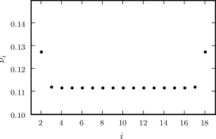
Refer to caption
Figure 11: Numerical solution to the stationary point condition Eq. (58) for a system with M=20𝑀20M=20, ϵ=10kBTditalic-ϵ10subscript𝑘𝐵𝑇𝑑\epsilon=10\>k_{B}Td, and Γ=400kBTdΓ400subscript𝑘𝐵𝑇𝑑\Gamma=400\>k_{B}Td. The solution is expressed in terms of νi=λiclϵ/d2subscript𝜈𝑖superscriptsubscript𝜆𝑖clitalic-ϵsuperscript𝑑2\nu_{i}=\lambda_{i}^{\text{cl}}-\epsilon/d^{2} for i=2,,M2𝑖2𝑀2i=2,\ldots,M-2, in units of kBT/dsubscript𝑘𝐵𝑇𝑑k_{B}T/d. The value of ν0/d=λ1clϵ/2d2=λM1clϵ/2d2subscript𝜈0𝑑superscriptsubscript𝜆1clitalic-ϵ2superscript𝑑2superscriptsubscript𝜆𝑀1clitalic-ϵ2superscript𝑑2\nu_{0}/d=\lambda_{1}^{\text{cl}}-\epsilon/2d^{2}=\lambda_{M-1}^{\text{cl}}-\epsilon/2d^{2} is 0.7831kBT/d0.7831subscript𝑘𝐵𝑇𝑑0.7831\>k_{B}T/d.

Unfortunately Eq. (63) is not analytically tractable, because the FMFsubscript𝐹MFF_{\text{MF}} given by Eq. (62) cannot be evaluated in closed form for an arbitrary function ν(s)𝜈𝑠\nu(s). On the other hand, the stationary point condition in the discrete system, Eq. (58) for F𝐹F in Eq. (55), can be solved numerically for small M𝑀M, and a representative set of νisubscript𝜈𝑖\nu_{i} are shown in Fig. 11 (for M=20𝑀20M=20, ϵ=10kBTditalic-ϵ10subscript𝑘𝐵𝑇𝑑\epsilon=10k_{B}Td, Γ=400kBTdΓ400subscript𝑘𝐵𝑇𝑑\Gamma=400k_{B}Td). For large Γϵmuch-greater-thanΓitalic-ϵ\Gamma\gg\epsilon, the νisubscript𝜈𝑖\nu_{i} are nearly constant for 2iM22𝑖𝑀22\leq i\leq M-2, and we can use this fact to make the following approximation in the continuum limit: replace ν(s)𝜈𝑠\nu(s) by a constant ν𝜈\nu in the Hamiltonian UMFsubscript𝑈MFU_{\text{MF}} of Eq. (62). Thus the first part of Eq. (63) becomes FMF/ν=0subscript𝐹MF𝜈0\partial F_{\text{MF}}/\partial\nu=0, implying a global constraint

L/2L/2𝑑s𝐮2(s)=(1+4ϵΓ)L,superscriptsubscript𝐿2𝐿2differential-d𝑠delimited-⟨⟩superscript𝐮2𝑠14italic-ϵΓ𝐿\int_{-L/2}^{L/2}ds\,\langle\mathbf{u}^{2}(s)\rangle=\left(1+\frac{4\epsilon}{\Gamma}\right)L\,, (65)

instead of the local constraint 𝐮2(s)=1+4ϵ/Γdelimited-⟨⟩superscript𝐮2𝑠14italic-ϵΓ\langle\mathbf{u}^{2}(s)\rangle=1+4\epsilon/\Gamma in Eq. (64).

This approximation, which becomes exact when ΓΓ\Gamma\to\infty, allows us to find a closed form expression for FMFsubscript𝐹MFF_{\text{MF}}. Using a mapping of the first two terms of UMFsubscript𝑈MFU_{\text{MF}} to the quantum mechanical harmonic oscillator (with mass m=ϵ𝑚italic-ϵm=\epsilon and frequency ω=2ν/ϵ𝜔2𝜈italic-ϵ\omega=\sqrt{2\nu/\epsilon}) [23], the path integral for FMFsubscript𝐹MFF_{\text{MF}} can be evaluated, giving the free energy

FMF=Lν2ν04LνϵΓ4ν0ϵΓ32β(log[βνϵcsch(L2νϵ)]log[β2(2ν02+νϵ)2+β2ν02νϵcoth(L2νϵ)]),subscript𝐹MF𝐿𝜈2subscript𝜈04𝐿𝜈italic-ϵΓ4subscript𝜈0italic-ϵΓ32𝛽𝛽𝜈italic-ϵcsch𝐿2𝜈italic-ϵsuperscript𝛽22superscriptsubscript𝜈02𝜈italic-ϵ2superscript𝛽2subscript𝜈02𝜈italic-ϵcoth𝐿2𝜈italic-ϵ\begin{split}&F_{\text{MF}}=-L\nu-2\nu_{0}-\frac{4L\nu\epsilon}{\Gamma}-\frac{4\nu_{0}\epsilon}{\Gamma}\\ &\quad-\frac{3}{2\beta}\left(\log\left[\beta\sqrt{\nu\epsilon}\,\text{csch}\left(L\sqrt{\frac{2\nu}{\epsilon}}\right)\right]\right.\\ &\quad-\left.\log\left[\frac{\beta^{2}(2\nu_{0}^{2}+\nu\epsilon)}{2}+\beta^{2}\nu_{0}\sqrt{2\nu\epsilon}\,\text{coth}\left(L\sqrt{\frac{2\nu}{\epsilon}}\right)\right]\right)\,,\end{split} (66)

up to an additive constant. Using Eq. (66), the stationary point condition FMF/ν=FMF/ν0=0subscript𝐹MF𝜈subscript𝐹MFsubscript𝜈00\partial F_{\text{MF}}/\partial\nu=\partial F_{\text{MF}}/\partial\nu_{0}=0 can be solved numerically for ν𝜈\nu and ν0subscript𝜈0\nu_{0} given L𝐿L, ϵitalic-ϵ\epsilon, and ΓΓ\Gamma. For Lϵmuch-greater-than𝐿italic-ϵL\gg\epsilon, the condition takes the simple limiting form,

νϵ2=34kBTΓΓ+4ϵ,ν0=34kBTΓ(Γ+6ϵ)(Γ+2ϵ)(Γ+4ϵ).formulae-sequence𝜈italic-ϵ234subscript𝑘𝐵𝑇ΓΓ4italic-ϵsubscript𝜈034subscript𝑘𝐵𝑇ΓΓ6italic-ϵΓ2italic-ϵΓ4italic-ϵ\begin{split}\sqrt{\frac{\nu\epsilon}{2}}&=\frac{3}{4}k_{B}T\frac{\Gamma}{\Gamma+4\epsilon}\,,\\ \nu_{0}&=\frac{3}{4}k_{B}T\frac{\Gamma(\Gamma+6\epsilon)}{(\Gamma+2\epsilon)(\Gamma+4\epsilon)}\,.\end{split} (67)

When ΓΓ\Gamma\to\infty, Eq. (67) reduces to Eq. (18) in Sec. 4, and this is generally true of the stationary point condition for any L𝐿L.

The equilibrium properties of the chain described by the Hamiltonian UMFsubscript𝑈MFU_{\text{MF}} can be calculated with a similar approach to the one used in Ref. 27, where distribution functions were derived for the Γ=Γ\Gamma=\infty mean-field model. The main result is G(s,s;𝐱;𝐮,𝐮)𝐺𝑠superscript𝑠𝐱𝐮superscript𝐮G(s,s^{\prime};\mathbf{x};\mathbf{u},\mathbf{u}^{\prime}), the probability density for finding two points on the chain at s𝑠s and ssuperscript𝑠s^{\prime} with s>ssuperscript𝑠𝑠s^{\prime}>s, having spatial separation 𝐫(s)𝐫(s)=𝐱𝐫superscript𝑠𝐫𝑠𝐱\mathbf{r}(s^{\prime})-\mathbf{r}(s)=\mathbf{x}, and tangent vectors 𝐮(s)=𝐮𝐮𝑠𝐮\mathbf{u}(s)=\mathbf{u}, 𝐮(s)=𝐮𝐮superscript𝑠superscript𝐮\mathbf{u}(s^{\prime})=\mathbf{u}^{\prime}. The full expression for this probability is

G(s,s;𝐱;𝐮,𝐮)=(A(s,s)4π3B4(ss))3/2exp[B1(ss)(𝐮2+𝐮2)+B2(ss)𝐮𝐮(𝐱B3(ss)(𝐮+𝐮))2B4(ss)C(s+L/2)𝐮2C(L/2s)𝐮2],𝐺𝑠superscript𝑠𝐱𝐮superscript𝐮superscript𝐴𝑠superscript𝑠4superscript𝜋3subscript𝐵4superscript𝑠𝑠32subscript𝐵1superscript𝑠𝑠superscript𝐮2superscriptsuperscript𝐮2subscript𝐵2superscript𝑠𝑠𝐮superscript𝐮superscript𝐱subscript𝐵3superscript𝑠𝑠𝐮superscript𝐮2subscript𝐵4superscript𝑠𝑠𝐶𝑠𝐿2superscript𝐮2𝐶𝐿2superscript𝑠superscriptsuperscript𝐮2\begin{split}&G(s,s^{\prime};\mathbf{x};\mathbf{u},\mathbf{u}^{\prime})=\\ &\quad\left(\frac{A(s,s^{\prime})}{4\pi^{3}B_{4}(s^{\prime}-s)}\right)^{3/2}\exp\Biggl{[}-B_{1}(s^{\prime}-s)(\mathbf{u}^{2}+{\mathbf{u}^{\prime}}^{2})\\ &\quad+B_{2}(s^{\prime}-s)\mathbf{u}\cdot\mathbf{u}^{\prime}-\frac{\left(\mathbf{x}-B_{3}(s^{\prime}-s)(\mathbf{u}+\mathbf{u}^{\prime})\right)^{2}}{B_{4}(s^{\prime}-s)}\\ &\quad-C(s+L/2)\mathbf{u}^{2}-C(L/2-s^{\prime}){\mathbf{u}^{\prime}}^{2}\Biggr{]}\,,\end{split} (68)

where the functions A(s)𝐴𝑠A(s), Bi(s)subscript𝐵𝑖𝑠B_{i}(s), i=1,,4𝑖14i=1,\ldots,4, and C(s)𝐶𝑠C(s) are given by

A(s,s)=4(B1(ss)+C(s+L/2))(B1(ss)+C(L/2s))B22(ss),B1(s)=βϵω2coth(sω),B2(s)=βϵωcsch(sω),B3(s)=ϵω2νtanh(sω2),B4(s)=sβνϵωβν2tanh(sω2),C(s)=βϵω(ϵω+2ν0coth(sω))4ν0+2ϵωcoth(sω),\begin{split}A(s,s^{\prime})&=4(B_{1}(s^{\prime}-s)+C(s+L/2))\\ &\quad\cdot(B_{1}(s^{\prime}-s)+C(L/2-s^{\prime}))-B_{2}^{2}(s^{\prime}-s)\,,\\ B_{1}(s)&=\frac{\beta\epsilon\omega}{2}\coth(s\omega)\,,\quad B_{2}(s)=\beta\epsilon\omega\,\text{csch}(s\omega)\,,\\ B_{3}(s)&=\frac{\epsilon\omega}{2\nu}\tanh\left(\frac{s\omega}{2}\right)\,,\\ B_{4}(s)&=\frac{s}{\beta\nu}-\frac{\epsilon\omega}{\beta\nu^{2}}\tanh\left(\frac{s\omega}{2}\right)\,,\\ C(s)&=\frac{\beta\epsilon\omega(\epsilon\omega+2\nu_{0}\,\text{coth}(s\omega))}{4\nu_{0}+2\epsilon\omega\,\text{coth}(s\omega)}\,,\end{split} (69)

with ω=2ν/ϵ𝜔2𝜈italic-ϵ\omega=\sqrt{2\nu/\epsilon}.

From G(s,s;𝐱;𝐮,𝐮)𝐺𝑠superscript𝑠𝐱𝐮superscript𝐮G(s,s^{\prime};\mathbf{x};\mathbf{u},\mathbf{u}^{\prime}) we can calculate other properties of the chain, for example the tangent vector correlation function 𝐮(s)𝐮(s)delimited-⟨⟩𝐮𝑠𝐮superscript𝑠\langle\mathbf{u}(s)\cdot\mathbf{u}(s^{\prime})\rangle for s>ssuperscript𝑠𝑠s^{\prime}>s,

𝐮(s)𝐮(s)=d3𝐱𝐮(s)𝐮(s)G(s,s;𝐱;𝐮(s),𝐮(s))=B2(ss)A(s,s).delimited-⟨⟩𝐮𝑠𝐮superscript𝑠superscript𝑑3𝐱𝐮𝑠𝐮superscript𝑠𝐺𝑠superscript𝑠𝐱𝐮𝑠𝐮superscript𝑠subscript𝐵2superscript𝑠𝑠𝐴superscript𝑠𝑠\begin{split}\langle\mathbf{u}(s)\cdot\mathbf{u}(s^{\prime})\rangle&=\int d^{3}\mathbf{x}\,\mathbf{u}(s)\cdot\mathbf{u}(s^{\prime})\,G(s,s^{\prime};\mathbf{x};\mathbf{u}(s),\mathbf{u}(s^{\prime}))\\ &=\frac{B_{2}(s^{\prime}-s)}{A(s^{\prime},s)}\,.\end{split} (70)

For Lϵmuch-greater-than𝐿italic-ϵL\gg\epsilon, L/2s,sL/2formulae-sequencemuch-less-than𝐿2𝑠much-less-thansuperscript𝑠𝐿2-L/2\ll s,s^{\prime}\ll L/2, Eq. (70) can be simplified using Eq. (67) for ν𝜈\nu and ν0subscript𝜈0\nu_{0}, giving

𝐮(s)𝐮(s)=(1+4ϵΓ)exp(3(ss)ΓkBT2ϵ(Γ+4ϵ)).delimited-⟨⟩𝐮𝑠𝐮superscript𝑠14italic-ϵΓ3superscript𝑠𝑠Γsubscript𝑘𝐵𝑇2italic-ϵΓ4italic-ϵ\langle\mathbf{u}(s)\cdot\mathbf{u}(s^{\prime})\rangle=\left(1+\frac{4\epsilon}{\Gamma}\right)\exp\left(-\frac{3(s^{\prime}-s)\Gamma k_{B}T}{2\epsilon(\Gamma+4\epsilon)}\right)\,. (71)

When ΓΓ\Gamma\to\infty, the tangent correlation function reduces to the Kratky-Porod form of Eq. (19), 𝐮(s)𝐮(s)=exp(3(ss)kBT/2ϵ)=exp((ss)/lp)delimited-⟨⟩𝐮𝑠𝐮superscript𝑠3superscript𝑠𝑠subscript𝑘𝐵𝑇2italic-ϵsuperscript𝑠𝑠subscript𝑙𝑝\langle\mathbf{u}(s)\cdot\mathbf{u}(s^{\prime})\rangle=\exp(-3(s^{\prime}-s)k_{B}T/2\epsilon)=\exp(-(s^{\prime}-s)/l_{p}).

Thus we have shown that a mean-field theory based on the extensible worm-like chain Hamiltonian used in the simulations gives results very similar to the MFT described in Sec. 4, with the finite extensibility leading to small corrections to the parameters of UMFsubscript𝑈MFU_{\text{MF}} on the order of ϵ/Γitalic-ϵΓ\epsilon/\Gamma.

Appendix B: Analytical Approximation for γnsubscript𝛾𝑛\gamma_{n} and δnsubscript𝛿𝑛\delta_{n}

In order to derive analytical expressions for the exponents γnsubscript𝛾𝑛\gamma_{n} and δnsubscript𝛿𝑛\delta_{n} from the MFT theory, we make several approximations in the derivation described in Sec. 4. Since the off-diagonal elements of the interaction matrix Hnmsubscript𝐻𝑛𝑚H_{nm} defined by Eq. (34) are smaller than the diagonal ones, we will treat them as a perturbation. To first order in the perturbation expansion, we can write the following expressions for τnsubscript𝜏𝑛\tau_{n}, ΘnsubscriptΘ𝑛\Theta_{n}, and Ψn(L/2)subscriptΨ𝑛𝐿2\Psi_{n}(L/2) when n>0𝑛0n>0:

τn=Λn1λn1Hnn1Hnn2λn1mnHnm2λmHnnλnHmmλm,ΘnHnn+2mnHnm2λmHnnλnHmmλm,Ψn(L/2)=mψm(L/2)(C1)mnψn(L/2)+1LH0nHnn+mnψm(L/2)HnmλnHnnλnHmmλm.formulae-sequencesubscript𝜏𝑛superscriptsubscriptΛ𝑛1superscriptsubscript𝜆𝑛1superscriptsubscript𝐻𝑛𝑛1superscriptsubscript𝐻𝑛𝑛2superscriptsubscript𝜆𝑛1subscript𝑚𝑛superscriptsubscript𝐻𝑛𝑚2subscript𝜆𝑚subscript𝐻𝑛𝑛subscript𝜆𝑛subscript𝐻𝑚𝑚subscript𝜆𝑚formulae-sequencesubscriptΘ𝑛subscript𝐻𝑛𝑛2subscript𝑚𝑛superscriptsubscript𝐻𝑛𝑚2subscript𝜆𝑚subscript𝐻𝑛𝑛subscript𝜆𝑛subscript𝐻𝑚𝑚subscript𝜆𝑚subscriptΨ𝑛𝐿2subscript𝑚subscript𝜓𝑚𝐿2subscriptsuperscript𝐶1𝑚𝑛subscript𝜓𝑛𝐿21𝐿subscript𝐻0𝑛subscript𝐻𝑛𝑛subscript𝑚𝑛subscript𝜓𝑚𝐿2subscript𝐻𝑛𝑚subscript𝜆𝑛subscript𝐻𝑛𝑛subscript𝜆𝑛subscript𝐻𝑚𝑚subscript𝜆𝑚\begin{split}\tau_{n}&=\Lambda_{n}^{-1}\approx\lambda_{n}^{-1}H_{nn}^{-1}-H_{nn}^{-2}\lambda_{n}^{-1}\sum_{m\neq n}\frac{H_{nm}^{2}\lambda_{m}}{H_{nn}\lambda_{n}-H_{mm}\lambda_{m}},\\ \Theta_{n}&\approx H_{nn}+2\sum_{m\neq n}\frac{H_{nm}^{2}\lambda_{m}}{H_{nn}\lambda_{n}-H_{mm}\lambda_{m}},\\ \Psi_{n}(L/2)&=\sum_{m}\psi_{m}(L/2)(C^{-1})_{mn}\approx\psi_{n}(L/2)+\sqrt{\frac{1}{L}}\frac{H_{0n}}{H_{nn}}+\sum_{m\neq n}\psi_{m}(L/2)\frac{H_{nm}\lambda_{n}}{H_{nn}\lambda_{n}-H_{mm}\lambda_{m}}.\end{split} (72)

From these expressions one can also calculate Δn=6kBTτnΘnΨn2(L/2)subscriptΔ𝑛6subscript𝑘𝐵𝑇subscript𝜏𝑛subscriptΘ𝑛superscriptsubscriptΨ𝑛2𝐿2\Delta_{n}=6k_{B}T\tau_{n}\Theta_{n}\Psi_{n}^{2}(L/2). The double integral for Hnmsubscript𝐻𝑛𝑚H_{nm} in Eq. (34) can be rewritten in terms of new variables h=ss𝑠superscript𝑠h=s-s^{\prime} and w=s+s𝑤𝑠superscript𝑠w=s+s^{\prime} as follows:

Hnm=2aμ0δnm+6πaμ0L/2L/2𝑑sL/2L/2𝑑sψn(s)Θ(|ss|2a)σ(|ss|)exp(6a2σ(|ss|))ψm(s)=2aμ0δnm+6πaμ02aL𝑑hL+hLh𝑑wψn(h+w2)1σ(h)exp(6a2σ(h))ψm(wh2).subscript𝐻𝑛𝑚2𝑎subscript𝜇0subscript𝛿𝑛𝑚6𝜋𝑎subscript𝜇0superscriptsubscript𝐿2𝐿2differential-d𝑠superscriptsubscript𝐿2𝐿2differential-dsuperscript𝑠subscript𝜓𝑛𝑠Θ𝑠superscript𝑠2𝑎𝜎𝑠superscript𝑠6superscript𝑎2𝜎𝑠superscript𝑠subscript𝜓𝑚superscript𝑠2𝑎subscript𝜇0subscript𝛿𝑛𝑚6𝜋𝑎subscript𝜇0superscriptsubscript2𝑎𝐿differential-dsuperscriptsubscript𝐿𝐿differential-d𝑤subscript𝜓𝑛𝑤21𝜎6superscript𝑎2𝜎subscript𝜓𝑚𝑤2\begin{split}H_{nm}&=2a\mu_{0}\delta_{nm}+\sqrt{\frac{6}{\pi}}a\mu_{0}\int_{-L/2}^{L/2}ds\int_{-L/2}^{L/2}ds^{\prime}\,\psi_{n}(s)\frac{\Theta(|s-s^{\prime}|-2a)}{\sqrt{\sigma(|s-s^{\prime}|)}}\exp\left(-\frac{6a^{2}}{\sigma(|s-s^{\prime}|)}\right)\psi_{m}(s^{\prime})\,\\ &=2a\mu_{0}\delta_{nm}+\sqrt{\frac{6}{\pi}}a\mu_{0}\int_{2a}^{L}dh\int_{-L+h}^{L-h}dw\,\psi_{n}\left(\frac{h+w}{2}\right)\frac{1}{\sqrt{\sigma(h)}}\exp\left(-\frac{6a^{2}}{\sigma(h)}\right)\psi_{m}\left(\frac{w-h}{2}\right)\,.\end{split} (73)

Since σ(h)=2lph2lp2(1eh/lp)𝜎2subscript𝑙𝑝2superscriptsubscript𝑙𝑝21superscript𝑒subscript𝑙𝑝\sigma(h)=2l_{p}h-2l_{p}^{2}(1-e^{-h/l_{p}}) can be approximated as σ(h)h2𝜎superscript2\sigma(h)\approx h^{2} for hlpmuch-less-thansubscript𝑙𝑝h\ll l_{p} and σ(h)2lph𝜎2subscript𝑙𝑝\sigma(h)\approx 2l_{p}h for hlpmuch-greater-thansubscript𝑙𝑝h\gg l_{p}, we can split up the hh integral above into two pieces:

Hnm2aμ0δnm+aμ0(Inm(1)+Inm(2)),subscript𝐻𝑛𝑚2𝑎subscript𝜇0subscript𝛿𝑛𝑚𝑎subscript𝜇0subscriptsuperscript𝐼1𝑛𝑚subscriptsuperscript𝐼2𝑛𝑚H_{nm}\approx 2a\mu_{0}\delta_{nm}+a\mu_{0}(I^{(1)}_{nm}+I^{(2)}_{nm}), (74)

where

Inm(1)=6π2alp𝑑h1hexp(6a2h2)L+hLh𝑑wψn(h+w2)ψm(wh2),Inm(2)=6πlpL𝑑h12lphexp(3a2lph)L+hLh𝑑wψn(h+w2)ψm(wh2).formulae-sequencesubscriptsuperscript𝐼1𝑛𝑚6𝜋superscriptsubscript2𝑎subscript𝑙𝑝differential-d16superscript𝑎2superscript2superscriptsubscript𝐿𝐿differential-d𝑤subscript𝜓𝑛𝑤2subscript𝜓𝑚𝑤2subscriptsuperscript𝐼2𝑛𝑚6𝜋superscriptsubscriptsubscript𝑙𝑝𝐿differential-d12subscript𝑙𝑝3superscript𝑎2subscript𝑙𝑝superscriptsubscript𝐿𝐿differential-d𝑤subscript𝜓𝑛𝑤2subscript𝜓𝑚𝑤2\begin{split}I^{(1)}_{nm}&=\sqrt{\frac{6}{\pi}}\int_{2a}^{l_{p}}dh\,\frac{1}{h}\exp\left(-\frac{6a^{2}}{h^{2}}\right)\int_{-L+h}^{L-h}dw\,\psi_{n}\left(\frac{h+w}{2}\right)\psi_{m}\left(\frac{w-h}{2}\right),\\ I^{(2)}_{nm}&=\sqrt{\frac{6}{\pi}}\int_{l_{p}}^{L}dh\,\frac{1}{\sqrt{2l_{p}h}}\exp\left(-\frac{3a^{2}}{l_{p}h}\right)\int_{-L+h}^{L-h}dw\,\psi_{n}\left(\frac{h+w}{2}\right)\psi_{m}\left(\frac{w-h}{2}\right).\end{split} (75)

To complete the approximation, we will estimate these integrals in the two mode regimes discussed in Sec. 6, one for the case nL/lpmuch-less-than𝑛𝐿subscript𝑙𝑝n\ll L/l_{p}, the other for nL/lpmuch-greater-than𝑛𝐿subscript𝑙𝑝n\gg L/l_{p}. Since the biggest perturbation contributions in Eq. (72) for τnsubscript𝜏𝑛\tau_{n}, ΘnsubscriptΘ𝑛\Theta_{n}, and Ψn(L/2)subscriptΨ𝑛𝐿2\Psi_{n}(L/2) come from states with m𝑚m in the vicinity of n𝑛n, it is sufficient to consider matrix elements Hmnsubscript𝐻𝑚𝑛H_{mn} for m𝑚m in the same mode regime as n𝑛n.

B.1. n,mL/lpmuch-less-than𝑛𝑚𝐿subscript𝑙𝑝n,m\ll L/l_{p} regime

In the limit of long chain lengths, where Llp,amuch-greater-than𝐿subscript𝑙𝑝𝑎L\gg l_{p},\>a, the functions ψn(s)subscript𝜓𝑛𝑠\psi_{n}(s) and constants αnsubscript𝛼𝑛\alpha_{n}, λnsubscript𝜆𝑛\lambda_{n} for 0<nL/lp0𝑛much-less-than𝐿subscript𝑙𝑝0<n\ll L/l_{p} in Eqs. (31) and (32) simplify to:

ψn(s){(1)(n1)/22Lsin(πnsL)nodd,(1)n/22Lcos(πnsL)neven,αnπnL,λn3kBTπ2n22lpL2.\begin{split}\psi_{n}(s)&\approx\begin{cases}(-1)^{(n-1)/2}\sqrt{\frac{2}{L}}\sin\left(\frac{\pi ns}{L}\right)&n\>\text{odd},\\ (-1)^{n/2}\sqrt{\frac{2}{L}}\cos\left(\frac{\pi ns}{L}\right)&n\>\text{even},\end{cases}\\ \alpha_{n}&\approx\frac{\pi n}{L},\quad\lambda_{n}\approx\frac{3k_{B}T\pi^{2}n^{2}}{2l_{p}L^{2}}\,.\end{split} (76)

Due to the symmetry of the ψn(s)subscript𝜓𝑛𝑠\psi_{n}(s) functions, the matrix elements Hnmsubscript𝐻𝑛𝑚H_{nm} are non-zero only when n𝑛n and m𝑚m are both odd or both even, so the perturbation expansions in Eq. (72) can be done independently for even and odd states. For simplicity, we will assume n𝑛n and m𝑚m are odd for the rest of the derivation. Carrying out the analogous approximation for even n𝑛n, m𝑚m, will lead to qualitatively similar final expressions for δnsubscript𝛿𝑛\delta_{n} and γnsubscript𝛾𝑛\gamma_{n}, with slight shifts in the numerical coefficients.

Plugging Eq. (76) into Eq. (75), we can approximately evaluate the integrals in the large L𝐿L limit:

Inm(1){46Lπ[2ae3/2lpe6a2/lp2+a6πerf(3/2)a6πerf(6a/lp)]nm,6π[E1(6a2/lp2)E1(3/2)]n=m,Inm(2){Llp26(n+m)(n+m)π3/2nm,6Lπlp(1n1/212πn3/2)212πn=m.subscriptsuperscript𝐼1𝑛𝑚cases46𝐿𝜋delimited-[]2𝑎superscript𝑒32subscript𝑙𝑝superscript𝑒6superscript𝑎2superscriptsubscript𝑙𝑝2𝑎6𝜋erf32𝑎6𝜋erf6𝑎subscript𝑙𝑝𝑛𝑚6𝜋delimited-[]subscript𝐸16superscript𝑎2superscriptsubscript𝑙𝑝2subscript𝐸132𝑛𝑚subscriptsuperscript𝐼2𝑛𝑚cases𝐿subscript𝑙𝑝26𝑛𝑚𝑛𝑚superscript𝜋32𝑛𝑚6𝐿𝜋subscript𝑙𝑝1superscript𝑛1212𝜋superscript𝑛32212𝜋𝑛𝑚\begin{split}I^{(1)}_{nm}&\approx\begin{cases}\frac{4\sqrt{6}}{L\sqrt{\pi}}\left[2ae^{-3/2}-l_{p}e^{-6a^{2}/l_{p}^{2}}+a\sqrt{6\pi}\,\text{erf}(\sqrt{3/2})-a\sqrt{6\pi}\,\text{erf}(\sqrt{6}a/l_{p})\right]&n\neq m,\\ \sqrt{\frac{6}{\pi}}\left[E_{1}\left(6a^{2}/l_{p}^{2}\right)-E_{1}\left(3/2\right)\right]&n=m,\end{cases}\\ I^{(2)}_{nm}&\approx\begin{cases}-\sqrt{\frac{L}{l_{p}}}\frac{2\sqrt{6}}{(n+m)(\sqrt{n}+\sqrt{m})\pi^{3/2}}&n\neq m,\\ \sqrt{\frac{6L}{\pi l_{p}}}\left(\frac{1}{n^{1/2}}-\frac{1}{2\pi n^{3/2}}\right)-2\sqrt{\frac{12}{\pi}}&n=m.\end{cases}\end{split} (77)

Plugging these results into Eq. (74) for Hnmsubscript𝐻𝑛𝑚H_{nm}, we can also estimate the sums involved in the perturbation expansion of Eq. (72):

mnHnm2λmHnnλnHmmλmLlp(108π+27π2186π7/2n3/2+126+72π163π186π7/2n5/2),mnψm(L/2)HnmλnHnnλnHmmλm2L[118(9+43)+9+(9+3)π27π2n7245π+43π216π3n2].formulae-sequencesubscript𝑚𝑛superscriptsubscript𝐻𝑛𝑚2subscript𝜆𝑚subscript𝐻𝑛𝑛subscript𝜆𝑛subscript𝐻𝑚𝑚subscript𝜆𝑚𝐿subscript𝑙𝑝108𝜋27superscript𝜋2186superscript𝜋72superscript𝑛3212672𝜋163𝜋186superscript𝜋72superscript𝑛52subscript𝑚𝑛subscript𝜓𝑚𝐿2subscript𝐻𝑛𝑚subscript𝜆𝑛subscript𝐻𝑛𝑛subscript𝜆𝑛subscript𝐻𝑚𝑚subscript𝜆𝑚2𝐿delimited-[]118943993𝜋27superscript𝜋2𝑛7245𝜋43𝜋216superscript𝜋3superscript𝑛2\begin{split}\sum_{m\neq n}\frac{H_{nm}^{2}\lambda_{m}}{H_{nn}\lambda_{n}-H_{mm}\lambda_{m}}&\approx\sqrt{\frac{L}{l_{p}}}\left(\frac{-108\pi+27\pi^{2}}{18\sqrt{6}\pi^{7/2}n^{3/2}}+\frac{-126+72\pi-16\sqrt{3}\pi}{18\sqrt{6}\pi^{7/2}n^{5/2}}\right),\\ \sum_{m\neq n}\psi_{m}(L/2)\frac{H_{nm}\lambda_{n}}{H_{nn}\lambda_{n}-H_{mm}\lambda_{m}}&\approx\sqrt{\frac{2}{L}}\left[\frac{1}{18}\left(-9+4\sqrt{3}\right)+\frac{-9+\left(9+\sqrt{3}\right)\pi}{27\pi^{2}n}-\frac{72-45\pi+4\sqrt{3}\pi}{216\pi^{3}n^{2}}\right].\end{split} (78)

Combining the results of Eqs. (72), (74), and (76)-(78), we can derive the following expressions for γnsubscript𝛾𝑛\gamma_{n} and δnsubscript𝛿𝑛\delta_{n}:

γn=dlogτndlogn=nτndτndn3p1(n)+5.07p2(n)nlpLK(6a2lp2)2p3(n)+2.89p4(n)nlpLK(6a2lp2),δn=dlogΔndlogn=nΔndΔndn2p5(n)+0.0393p6(n)lpnLK(6a2lp2)p7(n)+0.0157p8(n)lpnLK(6a2lp2),formulae-sequencesubscript𝛾𝑛𝑑subscript𝜏𝑛𝑑𝑛𝑛subscript𝜏𝑛𝑑subscript𝜏𝑛𝑑𝑛3subscript𝑝1𝑛5.07subscript𝑝2𝑛𝑛subscript𝑙𝑝𝐿𝐾6superscript𝑎2superscriptsubscript𝑙𝑝22subscript𝑝3𝑛2.89subscript𝑝4𝑛𝑛subscript𝑙𝑝𝐿𝐾6superscript𝑎2superscriptsubscript𝑙𝑝2subscript𝛿𝑛𝑑subscriptΔ𝑛𝑑𝑛𝑛subscriptΔ𝑛𝑑subscriptΔ𝑛𝑑𝑛2subscript𝑝5𝑛0.0393subscript𝑝6𝑛subscript𝑙𝑝𝑛𝐿𝐾6superscript𝑎2superscriptsubscript𝑙𝑝2subscript𝑝7𝑛0.0157subscript𝑝8𝑛subscript𝑙𝑝𝑛𝐿𝐾6superscript𝑎2superscriptsubscript𝑙𝑝2\begin{split}\gamma_{n}&=-\frac{d\log\tau_{n}}{d\log n}=-\frac{n}{\tau_{n}}\frac{d\tau_{n}}{dn}\approx\frac{3p_{1}(n)+5.07p_{2}(n)\sqrt{\frac{nl_{p}}{L}}K\left(\frac{6a^{2}}{l_{p}^{2}}\right)}{2p_{3}(n)+2.89p_{4}(n)\sqrt{\frac{nl_{p}}{L}}K\left(\frac{6a^{2}}{l_{p}^{2}}\right)},\\ \delta_{n}&=-\frac{d\log\Delta_{n}}{d\log n}=-\frac{n}{\Delta_{n}}\frac{d\Delta_{n}}{dn}\approx\frac{2p_{5}(n)+0.0393p_{6}(n)\sqrt{\frac{l_{p}}{nL}}K\left(\frac{6a^{2}}{l_{p}^{2}}\right)}{p_{7}(n)+0.0157p_{8}(n)\sqrt{\frac{l_{p}}{nL}}K\left(\frac{6a^{2}}{l_{p}^{2}}\right)},\\ \end{split} (79)

where

K(x)6π(E1(x)E1(3/2))43π+2,𝐾𝑥6𝜋subscript𝐸1𝑥subscript𝐸13243𝜋2K(x)\equiv\sqrt{\frac{6}{\pi}}\left(E_{1}(x)-E_{1}(3/2)\right)-4\sqrt{\frac{3}{\pi}}+2, (80)

and p1(n),,p8(n)subscript𝑝1𝑛subscript𝑝8𝑛p_{1}(n),\ldots,p_{8}(n) are polynomials in n𝑛n of the form pi(n)=1+ai/n+bi/n2+subscript𝑝𝑖𝑛1subscript𝑎𝑖𝑛subscript𝑏𝑖superscript𝑛2p_{i}(n)=1+a_{i}/n+b_{i}/n^{2}+\cdots. The first two coefficients aisubscript𝑎𝑖a_{i} and bisubscript𝑏𝑖b_{i} are given in the following table:

i𝑖i 1 2 3 4 5 6 7 8
aisubscript𝑎𝑖a_{i} -0.176 -0.0919 -0.297 -0.148 0.282 0.608 0.188 0.435
bisubscript𝑏𝑖b_{i} -0.00186 -0.00504 0.0179 -0.00196 0.0440 0.185 0.0220 0.103
Table 1: Coefficients aisubscript𝑎𝑖a_{i} and bisubscript𝑏𝑖b_{i} of polynomials pi(n)=1+ai/n+bi/n2+subscript𝑝𝑖𝑛1subscript𝑎𝑖𝑛subscript𝑏𝑖superscript𝑛2p_{i}(n)=1+a_{i}/n+b_{i}/n^{2}+\cdots.

B.2. n,mL/lpmuch-greater-than𝑛𝑚𝐿subscript𝑙𝑝n,m\gg L/l_{p} regime

With the assumptions that Llpmuch-greater-than𝐿subscript𝑙𝑝L\gg l_{p} and lpamuch-greater-thansubscript𝑙𝑝𝑎l_{p}\gg a, the functions ψn(s)subscript𝜓𝑛𝑠\psi_{n}(s) and constants αnsubscript𝛼𝑛\alpha_{n}, λnsubscript𝜆𝑛\lambda_{n} for nL/lpmuch-greater-than𝑛𝐿subscript𝑙𝑝n\gg L/l_{p} in Eqs. (31) and (32) become:

ψn(s){(1)(n1)/22Lsin(π(2n1)s2L)+1Lsinh(π(2n1)s/2L)cosh(π(2n1)/4)nodd,(1)n/22Lcos(π(2n1)s2L)+1Lcosh(π(2n1)s/2L)sinh(π(2n1)/4)neven,αnπ(2n1)2L,λn3kBTlpπ4(2n1)432L4.\begin{split}\psi_{n}(s)&\approx\begin{cases}(-1)^{(n-1)/2}\sqrt{\frac{2}{L}}\sin\left(\frac{\pi(2n-1)s}{2L}\right)+\sqrt{\frac{1}{L}}\frac{\sinh\left(\pi(2n-1)s/2L\right)}{\cosh\left(\pi(2n-1)/4\right)}&n\>\text{odd},\\ (-1)^{n/2}\sqrt{\frac{2}{L}}\cos\left(\frac{\pi(2n-1)s}{2L}\right)+\sqrt{\frac{1}{L}}\frac{\cosh\left(\pi(2n-1)s/2L\right)}{\sinh\left(\pi(2n-1)/4\right)}&n\>\text{even},\end{cases}\\ \alpha_{n}&\approx\frac{\pi(2n-1)}{2L},\quad\lambda_{n}\approx\frac{3k_{B}Tl_{p}\pi^{4}(2n-1)^{4}}{32L^{4}}.\end{split} (81)

Again we will focus for simplicity on the case of odd n𝑛n and m𝑚m. For n,mL/lpmuch-greater-than𝑛𝑚𝐿subscript𝑙𝑝n,m\gg L/l_{p}, the first integral in Eq. (75) dominates, Inm(1)Inm(2)much-greater-thansuperscriptsubscript𝐼𝑛𝑚1superscriptsubscript𝐼𝑛𝑚2I_{nm}^{(1)}\gg I_{nm}^{(2)}, so we can write Hnm2aμ0δnm+aμ0Inm(1)subscript𝐻𝑛𝑚2𝑎subscript𝜇0subscript𝛿𝑛𝑚𝑎subscript𝜇0subscriptsuperscript𝐼1𝑛𝑚H_{nm}\approx 2a\mu_{0}\delta_{nm}+a\mu_{0}I^{(1)}_{nm}. The integral Inm(1)superscriptsubscript𝐼𝑛𝑚1I_{nm}^{(1)} can be approximated as:

Inm(1){26π3/2(m2+n2)(log(16a2mnπ2L2)+2γ)(m+n1)(m+n)2π(m+n1)(m+n)(m2+n2)nm,6nπ3/2[3+nπ{3γ+E1(32)+2log(6aπnL)}]n=m,subscriptsuperscript𝐼1𝑛𝑚cases26superscript𝜋32superscript𝑚2superscript𝑛216superscript𝑎2𝑚𝑛superscript𝜋2superscript𝐿22𝛾𝑚𝑛1superscript𝑚𝑛2𝜋𝑚𝑛1𝑚𝑛superscript𝑚2superscript𝑛2𝑛𝑚6𝑛superscript𝜋32delimited-[]3𝑛𝜋3𝛾subscript𝐸13226𝑎𝜋𝑛𝐿𝑛𝑚I^{(1)}_{nm}\approx\begin{cases}\frac{2\sqrt{6}}{\pi^{3/2}}\frac{\left(m^{2}+n^{2}\right)\left(\log\left(\frac{16a^{2}mn\pi^{2}}{L^{2}}\right)+2\gamma\right)-(m+n-1)(m+n)^{2}\pi}{(m+n-1)(m+n)\left(m^{2}+n^{2}\right)}&n\neq m,\\ -\frac{\sqrt{6}}{n\pi^{3/2}}\left[3+n\pi\left\{3\gamma+E_{1}\left(\frac{3}{2}\right)+2\log\left(\frac{\sqrt{6}a\pi n}{L}\right)\right\}\right]&n=m,\end{cases} (82)

where γ0.5772𝛾0.5772\gamma\approx 0.5772 is Euler’s constant. The resulting sums in the perturbation expansion of Eq. (72) are:

mnHnm2λmHnnλnHmmλm126nπ(3+A12log(Lanπ)),mnψm(L/2)HnmλnHnnλnHmmλm2L(13+A12log(Lanπ)),formulae-sequencesubscript𝑚𝑛superscriptsubscript𝐻𝑛𝑚2subscript𝜆𝑚subscript𝐻𝑛𝑛subscript𝜆𝑛subscript𝐻𝑚𝑚subscript𝜆𝑚126𝑛𝜋3𝐴12𝐿𝑎𝑛𝜋subscript𝑚𝑛subscript𝜓𝑚𝐿2subscript𝐻𝑛𝑚subscript𝜆𝑛subscript𝐻𝑛𝑛subscript𝜆𝑛subscript𝐻𝑚𝑚subscript𝜆𝑚2𝐿13𝐴12𝐿𝑎𝑛𝜋\begin{split}\sum_{m\neq n}\frac{H_{nm}^{2}\lambda_{m}}{H_{nn}\lambda_{n}-H_{mm}\lambda_{m}}&\approx\frac{12\sqrt{6}}{n\sqrt{\pi}\left(3+A-12\log\left(\frac{L}{an\pi}\right)\right)},\\ \sum_{m\neq n}\psi_{m}(L/2)\frac{H_{nm}\lambda_{n}}{H_{nn}\lambda_{n}-H_{mm}\lambda_{m}}&\approx\frac{2}{\sqrt{L}}\left(\frac{1}{3+A-12\log\left(\frac{L}{an\pi}\right)}\right),\end{split} (83)

where the constant A=18γ26π+6E1(32)+6log(6)13.06𝐴18𝛾26𝜋6subscript𝐸1326613.06A=18\gamma-2\sqrt{6\pi}+6E_{1}\left(\frac{3}{2}\right)+6\log(6)\approx 13.06. This yields the following expressions for γnsubscript𝛾𝑛\gamma_{n} and δnsubscript𝛿𝑛\delta_{n}:

γn4+12A12log(Lanπ),δn4+24(3+A12log(Lanπ))(5+A12log(Lanπ)).formulae-sequencesubscript𝛾𝑛412𝐴12𝐿𝑎𝑛𝜋subscript𝛿𝑛4243𝐴12𝐿𝑎𝑛𝜋5𝐴12𝐿𝑎𝑛𝜋\gamma_{n}\approx 4+\frac{12}{A-12\log\left(\frac{L}{an\pi}\right)},\quad\delta_{n}\approx 4+\frac{24}{\left(3+A-12\log\left(\frac{L}{an\pi}\right)\right)\left(5+A-12\log\left(\frac{L}{an\pi}\right)\right)}. (84)

References

  • [1] Lumma, D.; Keller, S.; Vilgis, T.; Rädler, J.O. Phys. Rev. Lett. 2003, 90, 218301.
  • [2] Shusterman, R.; Alon, S.; Gavrinyov, T.; Krichevsky, O. Phys. Rev. Lett. 2004, 92, 048303.
  • [3] Winkler, R. G.; Keller, S.; Rädler, J.O. Phys. Rev. E 2006, 73, 041919.
  • [4] Bernheim-Groswasser, A.; Shusterman, R.; Krichevsky, O. J. Chem. Phys 2006, 125, 084903.
  • [5] Petrov, E. P.; Ohrt, T.; Winkler, R. G.; Schwille, P. Phys. Rev. Lett. 2006, 97, 258101.
  • [6] Zimm, B. H. J. Chem. Phys. 1956, 24, 269.
  • [7] Doi, M.; Edwards, S. F. The Theory of Polymer Dynamics; Clarendon Press: Oxford, 1986.
  • [8] Lisy, V.; Tothova, J.; Zatovsky, A. Cond. Matt. Phys. 2006, 9, 95.
  • [9] Harnau, L.; Winkler, R. G.; Reineker, P. J. Chem. Phys. 1996, 104, 6355.
  • [10] Kroy, K.; Frey, E. Phys. Rev. E 1997, 55, 3092.
  • [11] Granek, R. J. Phys. II 1997, 7, 1761.
  • [12] Rubinstein M.; Colby, R. H. Polymer Physics; Oxford University Press: Oxford, 2003; pp. 322-334.
  • [13] Morse, D. C. Phys. Rev. E 1998, 58, R1237.
  • [14] Gittes, F.; MacKintosh, F. C. Phys. Rev. E 1998, 58, R1241.
  • [15] Everaers, R.; Jülicher, F.; Ajdari, A.; Maggs, A. C. Phys. Rev. Lett. 1999, 82, 3717.
  • [16] Schlagberger, X.; Bayer, J.; Rädler, J. O.; Netz, R. R. Europhys. Lett. 2006, 76, 346.
  • [17] Tirado, M. M.; Martinez, C.; Garcia, J. J. Chem. Phys. 1984, 81, 2047.
  • [18] Netz, R. R.; Andelman, D. Phys. Rep. 2003, 380, 1.
  • [19] Ermak, D. L.; Rapport d’activité scientifique du CECAM 1976, pp. 66-81.
  • [20] Ermak, D. L.; McCammon, J. A. J. Chem. Phys. 1978, 69, 1352.
  • [21] Rotne, J.; Prager, S. J. Chem. Phys. 1969, 50, 4831.
  • [22] Kratky, O.; Porod, G. Recl. Trav. Chim. Pays-Bas 1949, 68, 1106.
  • [23] Ha, B.-Y.; Thirumalai, D. J. Chem. Phys. 1995, 103, 9408.
  • [24] Ha, B.-Y.; Thirumalai, D. J. Chem. Phys. 1997, 106, 4243.
  • [25] Lagowski, J. B.; Noolandi, J.; Nickel, B. J. Chem. Phys. 1991, 95, 1266.
  • [26] Harris, R. A.; Hearst, J. E. J. Chem. Phys. 1966, 44, 2595.
  • [27] Winkler, R. G.; Reineker, P.; Harnau, L. J. Chem. Phys. 1994, 101, 8119.
  • [28] Dertinger, T.; Pacheco V; von der Hocht, I.; Hartmann, R.; Gregor, I.; Enderlein, J. ChemPhysChem 2007, 8, 433.
  • [29] Farge, E.; Maggs, A. C. Macromolecules 1993, 26, 5041.
  • [30] Dimitrakopoulos, P. J. Chem. Phys. 2003, 119, 8189.
  • [31] Dimitrakopoulos, P. Phys. Rev. Lett. 2004, 93, 217801.
  • [32] Piekenbrock, Th.; Sackmann, E. Biopolymers 1992, 32, 1471.
  • [33] Gisler, T.; Weitz, D. A. Phys. Rev. Lett. 1999, 82, 1606.
  • [34] Wong, I. Y.; Gardel, M. L.; Reichman, D. R.; Weeks, E. R.; Valentine, M. T.; Bausch, A. R.; Weitz, D. A. Phys. Rev. Lett. 2004, 92, 178101.
  • [35] Xu, J. Y.; Palmer, A.; Wirtz, D. Macromolecules 1998, 31, 6486.
  • [36] Caspi, A.; Elbaum, M.; Granek, R.; Lachish, A.; Zbaida, D. Phys. Rev. Lett. 1998, 80, 1106.