• The Use of the Long Baseline Array in Australia for Precise Geodesy and Absolute Astrometry

  ^A   Corresponding author: E-mail:

  Received 2008 October 29, accepted 2009 January 12

  Abstract: We report the results of a successful 12 hour 22 GHz VLBI experiment using a heterogeneous network that includes radio telescopes of the Long Baseline Array (LBA) in Australia and several VLBI stations that regularly observe in geodetic VLBI campaigns. We have determined positions of three VLBI stations, atca-104, ceduna and mopra, with an accuracy of 4–30 mm using a novel technique of data analysis. These stations have never before participated in geodetic experiments. We observed 105 radio sources, and amongst them 5 objects which have not previously been observed with VLBI. We have determined positions of these new sources with the accuracy of 2–5 mas. We make conclusion that the LBA network is capable of conducting absolute astrometry VLBI surveys with accuracy better than 5 mas.

  Keywords: instrumentation: interferometers — techniques: interferometric — reference systems

1 Introduction

The method of very long baseline interferometry (VLBI) first proposed by Matveenko, Kardashev, & Sholomitsky (1965) is widely used for geodesy and absolute astrometry. The first dedicated geodetic experiment on 1969 January 11 provided results with 1 meter accuracy (Hinteregger et al. 1972). In the following decades VLBI technology has flourished, sensitivities and accuracies have improved by several orders of magnitude and arrays of dedicated antennas have been built. Nowadays, a network of $\sim\!30$ stations spread over the globe participates regularly in observing programs for the Earth orientation parameters (EOP) monitoring, determination of source coordinates, deriving site positions, and monitoring their changes. These activities are coordinated by the International VLBI Services for Astrometry and Geodesy (IVS) (Schlüter & Behrend 2007).

However, the station distribution over the globe is non-uniform. The majority of radio telescopes are located in the northern hemisphere. This non-uniformity results in a disparity in the density of source catalogues: the number of sources with positions determined at a milliarcsecond level of accuracy in the declination zone $[-90^{\circ},-50^{\circ}]$ is a factor of 5 less than in the zone $[+50^{\circ},+90^{\circ}]$. Disparity in station distribution also results in the appearance of systematic errors in the EOP time series derived from analysis of VLBI observations at this network. Therefore, an increase of the number of observing stations in the southern hemisphere that are able to participate in VLBI observing campaigns under geodesy, absolute astrometry, and space navigation programs is very important.

There are seven radio telescopes in Australia that have VLBI recording equipment: hobart26, parkes, tidbin64, dss45, Australia Telescope Compact Array (atca), ceduna, mopra, and they potentially can participate in VLBI observing campaigns for astrometry and geodesy. The first four stations are equipped with Mark-4/Mark-5 data acquisition system and they have participated in many IVS observing programs. The last three stations have the Long Baseline Array Data Recorder (LBADR) data acquisition system that is not directly compatible with Mark-4/Mark-5 and they have never before participated in experiments for geodesy and absolute astrometry. Using all stations together is a challenging problem.

The possibility to use sensitive antennas ceduna, atca, mopra for space navigation and astrometry would significantly boost our capabilities to observe objects in the southern hemisphere. On 2005 January 16 stations atca-104, ceduna, mopra and parkes joined the global VLBI network that also included gbt, eight VLBA stations kashima, seshan25, and urumqi in the Huygens probe tracking observations during its descent in the atmosphere of Titan (Pogrebenko et al. 2004; Witasse et al. 2006). Detection of the Huygens probe signal on the North America–Australia baselines was crucial for the reconstruction of the probe trajectory with $\sim\!1$ km accuracy at Saturn’s distance of 1.3 billion km, although the uncertainty of the LBA station a priori coordinates introduced systematic errors in the probe’s positioning. A better a posteriori determination of the site coordinates was required to improve the accuracy of the probe’s trajectory reconstruction.

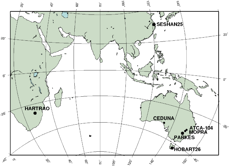
Figure 2: The network of VLBI stations that participated in the experiment on 2007 June 24. Stations with coordinates known from analysis of prior experiments are shown with big disks.

The Long Baseline Array incorporates 5 main antenna: the parkes 64 m, the mopra 22 m, the hobart 26 m, the ceduna 30 m, and the Australia Telescope Compact Array which consists of six 22 m antennas. When ATCA participate in VLBI observations, it can run as a phased array or, alternatively, only one of its antennas can be used. Antennas from the NASA’s Deep Space Network at the Canberra Deep Space Communication Complex, tidbin64 and dss45, regularly join the array as does the hartrao 26 m dish in South Africa. The array is used for source imaging, differential astrometry and other applications.

Imaging weak target sources and precise differential astrometry require a catalogue of compact calibrators with the density at least one object within a circle of 2–3^∘ of any direction. A catalogue of such calibrators was created from analysis of the VLBA Calibrator Survey observing campaign (Beasley et al. 2002; Fomalont et al. 2003; Petrov et al. 2005, 2006, 2008a; Kovalev et al. 2007). However, the VLBA cannot see objects with declinations below $-50^{\circ}$. The extension of the Calibrator Survey to the southern hemisphere should be derived from analysis of dedicated LBA observing campaigns.

For investigating the possibility of using the LBA antennas for precise geodesy and absolute astrometry we ran two observing sessions: a 1.5 hour long test VLBI experiment and a 12 hour geodetic VLBI experiment. The goal of these experiments was 1) to determine positions of atca, ceduna, mopra with the position accuracy 1–5 cm; 2) to evaluate the feasibility of running absolute astrometry observing campaigns with the heterogeneous LBA network.

In this paper we present results of these experiments. In Section 2 we describe the experiments, scheduling strategies and the hardware configuration. In Section 3 we describe the way how the heterogeneous data were transformed to the same format, transmitted to the correlator and correlated. In Section 4 we describe the algorithm for data analysis and present our results. Concluding remarks are given in section 5.

2 Observations

On 2006 May 16, stations atca-104, ceduna, mopra, hobart26, parkes ran a 1.5 hour long fringe test experiment at 22 GHz. The purpose of the fringe experiment was to test the data path, to test the frequency selection, to detect fringes, and to test data analysis procedure. Stations atca-104, ceduna, mopra recorded with the LBADR system. Data from these stations were converted into Mark-4 format using software developed at Metsähovi Radio Observatory for the Huygens VLBI experiment, then the data were test-correlated at the Joint Institute of VLBI in Europe, Dwingeloo (JIVE) in Dwingeloo, the Netherlands, and finally correlated at the Mark-4 correlator at the MPIfR in Bonn,Germany. Fringes were found at all baselines, except baselines with ceduna. Results from this test run allowed us to determine coarse positions of atca-104 and mopra, which helped to improve noticeably the Huygens VLBI trajectory reconstruction and encouraged us to run to a full-scale 22 GHz LBA experiment in the geodetic mode.

The telescopes atca-104, ceduna, hartrao, hobart26, mopra, parkes, and seshan25 (Figure 2) took part in the 12 hour experiment on 2007 June 24. Only one antenna of the 6-element ATCA array participated in the experiment. Antennas of the ATCA array can move along railroad tracks and can be positioned at one of 45 fixed station pads within 6 km range. The ATCA antenna that was used in the observations was positioned at the station pad CATW104, and it is referred to as atca-104.

This experiment was very different from routine geodetic VLBI experiments.

• We chose to observe at the K band (22 GHz). Traditionally, geodetic experiments are made in a dual-band mode when emission at S band (2.3 GHz) and X band (8.4 GHz) is recorded simultaneously. The linear combination of delays at the X and S bands is almost entirely free from the contribution of the ionosphere. The antennas atca-104, ceduna, mopra do not have dual-band S/X receivers, so we are limited to only one band. The highest frequency band that all antennas can receive is 22 GHz. Since the ionosphere contribution to group delay is reciprocal to the square of frequency, the ionosphere contribution at the K band is one order of magnitude smaller than the contribution at the X band. Our analysis of K band astrometry observations with the VLBA and several K band geodetic experiments with the Japanese VLBI interferometer network VERA showed that the ionospheric contribution at this frequency during the period of low solar activity is negligible, and the overall quality of geodetic results turned out even better than of dual band S/X observations.

• The digital backend used at atca, mopra and parkes allows recording of only two pairs of adjacent 16 MHz intermediate frequency channels (IF) in right circular polarization and the two pairs of adjacent frequency channels in the left circular polarization. ceduna can record only two pairs of adjacent IFs in one polarization. Although the IFs are recorded independently, the system effectively records emission from four channels and always records dual polarization (except ceduna), effectively giving only two 32 MHz channels at different frequencies at each polarization. This differs significantly from other VLBI backends such as the Mark-4/Mark-5 and K5 systems which support up to 32 frequency channels and the VLBA recording system which supports up to 8 frequency channels. Traditionally, from 4 to 16 channels per band are allocated. The frequency sequence is selected to minimize the power of sidelobes at the delay resolution function and for avoiding possible radio interferences. No geodetic experiments have ever been made with only two channels.

  The frequency sequence that we have chosen for this experiment is shown in Table 2. The frequency difference between two effective 32 MHz channels is 224 MHz. Since the accuracy of group delay determination observed at two effective intermediate frequency channels is reciprocal to the frequency separation, the wider the frequency separation, the better. From the other hand, the wider the separation of two effective IFs, the smaller group delay ambiguity spacing that is also reciprocal to the minimum frequency separation between separate frequency channels. The group delay ambiguity spacing in traditional VLBI experiments ranges from 28.5 ns to 200 ns. The spacings were 1/224 MHz = 4.5 ns in our experiment! Although the theoretical model for VLBI path delay has truncation errors less than 0.1 ps, the accuracy of delay prediction is limited to the accuracy of a priori parameters of the model. The major uncertainty of the a priori model arises from the contribution of the wet component of the tropospheric path delay that currently has a typical accuracy of 3–10 ns — higher than the group group delay ambiguity spacings. Therefore, traditional methods of data analysis that use group delays would fail.

  Table 2: The range of sky frequencies at four frequency channels in the observing session of 2007.06.24, in GHz.

  FC1	22.300 — 22.316
  FC2	22.316 — 22.332
  FC3	22.524 — 22.540
  FC4	22.540 — 22.556

• All stations, except ceduna, recorded both right circular polarization (RCP) and left circular polarization (LCP). Traditionally, only the RCP is recorded in geodetic experiments. Since the thermal noise of RCP and LCP data is independent, the use of LCP data reduces random errors of parameter estimates.

• The experiment had a heterogeneous setup. Data were recorded at 512 Mbit/s, 2 bit sampling, 16 MHz bandwidth per IF, 8 IFs, dual circular polarization (except from ceduna that can record only RCP). hobart26, hartrao and seshan25 used a Mark-4 data acquisition terminals with the setup shown above and wrote data onto disks using the Mark-5a VLBI recorder (Whitney 2005). The rest of the antennas used digital data acquisition system and the LBADR VLBI recorder which is a derivative of the PCEVN (Parsley et al. 2003). Data were recorded as 16 parallel bit streams. The LBADR uses different physical media for recording than the Mark-5a.

The LBADR system uses the VLBI Standard Interface (VSI–H) (A. Whitney 2000, unpublished internal document) signaling and connector conventions. Output bit streams from the VLBI digital backend are converted to the VSI–H using the universal VSI converter board called “VSIC” and captured into regular files on a server-grade PC run under Linux with a VSI–H–to–PCI record board called “VSIB”. To ensure sufficiently high data record rates, Linux software ”raid0” disk sets were used to store the recorded files. This is different from Mark-5 which uses proprietary disk modules as its physical media for recording.

To achieve compatibility with the correlator Mark-5 playback systems, two software solutions were used. The LBADR data of the first 1.5 hour fringe test run were software transformed to Mark-4 format, maintaining timecode information, using custom software running on a computer at JIVE. The resulting files were transferred to a Mark-5a unit to record disk modules for the Bonn correlator.

For the subsequent 12 hour run, software was developed that converts on-the-fly the raw LBADR data to Mark-5b format then sends the data using a tuned TCP stack over the network directly to files residing on a data server at JIVE. Mark-5b compatible disk modules were created and shipped from JIVE to Bonn for correlation. For future such experiments, the LBADR system will write Mark-5b data format directly, but will still not write to Mark-5 diskpacks.

2.1 Scheduling

The input list for automatic scheduling consists of 129 compact radio sources. This list was generated by merging two lists for different declination bands. Sources in the declination band [$-30^{\circ}$, $+40^{\circ}$] were selected from the catalogue of the 252 objects observed at K and Q band with the VLBA in 2002–2006 in the framework of the K/Q astrometric survey (Fey et al. 2005; Jacobs et al. 2005). They have the median K band correlated flux density $>0.4$ Jy at baselines longer than 5000 km. Sources in the declination band [$-90^{\circ}$, $-30^{\circ}$] were taken from the list of sources that were a) observed in geodetic VLBI experiments, b) observed and successfully imaged in astronomy experiments (Ojha et al. 2004), and c) have the median X band correlated flux density $>0.4$ Jy at baselines longer than 5000 km.

Automatic scheduling was made with the program SKED developed at the NASA GSFC by N. Vandenberg and J. Gipson (Petrov et al. 2008b). The algorithm for automatic scheduling generated a sequence of scans, i.e. intervals of time of 120 s duration when all antennas of the array, or a portion of the array, are pointed to a specific source and record the emission. Since the list of sources has 129 objects, there exists a very large number of possible sequences. SKED selected the sequence that optimizes the sky coverage at each individual station and minimizes the slew time needed for re-pointing antennas at the next source of the sequence. At each step of generating the sequence of scans, the software finds the distance of a candidate source from all previous sources scheduled within one hour. The candidate source with the largest minimum distance from all previous sources gets the highest sky-coverage score. SKED computes the slewing time and assigns weights to all candidate sources according to their scores based on sky-coverage, slewing time and some other optimization criteria. The source with the highest weight is put into the schedule. The scheduling algorithm adjusts weights to low elevation sources in such a way that each station observes at least one low elevation source every hour. The elevation cutoff was $12^{\circ}$ for all the stations, except parkes, that cannot slew lower than $31^{\circ}$ above the horizon.

SKED automatically selected 100 sources. In addition to them, five bright flat-spectrum sources from the Parkes Quarter-Jansky catalogue (Jackson et al. 2002) were inserted in the schedule manually at stations atca-104, ceduna, mopra, hobart25, parkes, two scans each. These sources have declination below $-55^{\circ}$ and have never been before observed with VLBI. The goal of including these sources in the schedule is to evaluate the feasibility of using the LBA for a search of new compact radio sources that can be used as calibrators for phase referencing observations.

3 Data Transmission and Correlation

Because of the media incompatibility of the LBADR and the Mark-5 format, as well as for convenience, data were transmitted using high speed networks between Australia and Europe. The data transmission was performed directly from the recorder PCs at the observatories in Australia, to a PC located at the JIVE. This was to utilize a dedicated 1 Gbps network which had previously been set up for eVLBI demonstrations as a part of the Express Production Real-time e-VLBI Service (EXPReS). The transmission was made using custom software which uses the TCP network protocol and has been tuned to efficiently use long, wide bandwidth networks. This software also performed an on-the-fly conversion of the LBADR data format to Mark-5b. This simply requires removing the LBADR headers and replacing them with Mark-5b headers (retaining time stamps) as the baseband bit format can be processed by Mark-4 correlators.

After transmission, the Mark-5b data were copied from the PC at JIVE to a Mark-5 disk-pack and shipped to Bonn correlator. Fringe checking was run on the EVN Mark-4 data processor at JIVE before the disk-packs were shipped to Bonn for final correlation. Those stations, that recorded with the Mark-5a data acquisition system, shipped the diskpacks with data to the correlator directly using air mail.

3.1 Correlation

The experiment was correlated at Bonn since the Bonn correlator has previously been thoroughly tested for astrometric and geodetic applications.

The Mark-4 correlator (Whitney et al. 2004) was configured to produce 512 lags and a 0.5 s accumulation period, to have as wide as possible delay and delay-rate fringe search window to allow for possible large station coordinate errors and source position errors. For comparison, the routine geodetic experiments use only 32 lags and accumulation periods of between 2 and 4 s since the errors in the a priori station and source positions are small. In this configuration, the correlator computing capacity is sufficient to process only four stations. Thus, we correlated six passes to form all the baselines between the seven antennas (with some redundancy). The selection of stations for correlation in each pass was guided only by the number of available Mark-5a and Mark-5b units at Bonn, but paying attention not to transpose data from the same antenna when correlating redundant baselines.

Since the LBA stations were not controlled by the Mark-4 field system software and therefore, they did not produce the observation log file required for correlation. Instead, the information required for the correlator control files, such as the scan name and scan times were recovered by comparing information from the Mark-5 module to the schedule file.

A trial correlation was performed to check the correctness of the correlator control files, for example clock offsets, frequencies, polarizations and track assignments. Quality control checks after each pass were made using the Haystack observatory post-processing system (HOPS) software package.

The stations did not inject phase calibration tones, so phase self calibration was applied to all stations in order to remove IF-dependent phase offsets at those stations with analogue data acquisition terminal (hobart26, hartrao, and seshan25). In the 17% of cases where the source was not detected on a baseline, those scans were re-correlated to ensure that these non-detections were not correlator artifacts.

Finally, the multi-band group delays and delay rates were adjusted using the fringe fitting algorithm implemented in HOPS program Fourfit in such a way, that applying these corrections to group delay and delay rate would maximized fringe amplitudes over each scan at each baseline independently.

4 Data Analysis

The fringe fit algorithm provides the estimates of fringe amplitudes, fringe phases, phase delay rates, narrow-band group delays, and multi-band group delays. Analysis of amplitude information provides the estimates of the correlated flux densities of observed sources and the sensitivity of antennas. Analysis of fringe phases and delays allows us to estimate station positions and source coordinates.

4.1 Position Analysis

Observed delays $\tau_{o}$ depend on an orientation of the baseline vector and the vector of source position, as well as propagation effects and clock functions. The differences between observed delay $\tau_{o}$ and predicted delay $\tau_{c}$ can be used for adjusting a vector of parameters $\Delta p$ using the least squares:

$$\displaystyle\sum_{i}\frac{\displaystyle\partial\tau}{\displaystyle\partial p_{i}}\Delta p_{i}=\tau_{o}-\tau_{c}.$$ (1)

The overview of the technique for computing predicted delays can be found in Sovers, Fanselow, & Jacobs CS (1998). We used the software library VTD for computing the theoretical path delay. The expression for time delay derived by Kopeikin & Schäfer (1999) in the framework of general relativity was used. The displacements caused by the Earth’s tides were computed using a rigorous algorithm of Petrov & Ma (2003) with a truncation at a level of 0.05 mm based on the numerical values of the generalized Love numbers presented by Mathews (2001). The displacements caused by ocean loading were computed by convolving the Greens’ functions with ocean tide models using the NLOADF algorithm of Agnew (1997). The GOT00 model (Ray 1999) of diurnal and semi-diurnal ocean tides, the NAO99 model (Matsumoto, Takanezawa, &  Ooe 2000) of ocean zonal tides, the equilibrium model of the pole tide and the tide with period of 18.6 years were used. The atmospheric pressure loading was computed by convolving the Greens’ functions with the output of the atmosphere NCEP Reanalysis numerical model (Kalnay et al. 1996). The algorithm of computations is described in full details in Petrov & Boy (2004).

The accuracy of the a priori model is not enough to resolve reliably multi-band group delays computed over the entire recorded bandwidth that have ambiguities with spacing 4.5 ns. The ambiguity spacing of narrow-band group delays, that were computed for each frequency channel separately and then averaged, is 16 mks, but the precision or narrow-band delays is worse by the ratio of the width of the entire recorded band to the width of the individual channel, i.e. a factor of 14. The uncertainties of narrow-band group delays are in the range of 0.05–10.0 ns. Of those, 78% fall within less than 0.8 nsec, i.e. 1/6 of the multi-band group delay ambiguity spacings for 78% observations. Therefore, a direct substitution of narrow-band delays to multi-band group delays will leave wrong ambiguities for 1/5 of the observations. The time-variable differences between narrow-band delays and multi-band delays due to instrumental effects will worsen the situation even further.

To circumvent the problem, we first made the solution using narrow-band group delays. The estimated parameters were coefficients of the 1st degree B-spline that model clock functions and atmosphere zenith path delay at each station, positions of the three new stations, atca-104, mopra, ceduna, coordinates of five new sources, the pole coordinates and the UT1 angle.

We formed new right-hand sides in a system of equations 1: $\tau^{gr}_{o}\>-\>\tau_{c}\>-\>\displaystyle\sum_{i}\frac{\displaystyle\partial\tau}{\displaystyle\partial p^{nb}_{i}}\Delta p^{nb}_{i}$, where $\tau^{gr}_{o}$ are multi-band observed group delays and $p^{nb}_{i}$ are parameter adjustments from the LSQ solution that used narrow-band delays. The accuracy of the a priori model with adjustments taken from the narrow-band delay solution turned out sufficient for reliable resolving group delay ambiguities at all baselines. The example of the differences between observed multi-band group delays and predicted are presented in Figures 4–6.

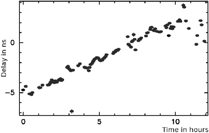
Figure 4: The differences between observed multi-band group delays and theoretical delays for baseline atca-104/ceduna predicted on the basis of the a priori model updated with results of the LSQ solution that used narrow-band delays.

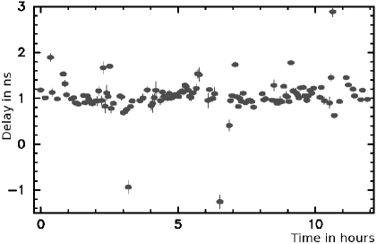
Figure 6: The differences between observed multi-band group delays and theoretical delays for baseline mopra/hobart26 predicted on the basis of the a priori model updated with results of the LSQ solution that used narrow-band delays.

During the preliminary fringe test, we used frequencies 23472, 23488, 23600, and 23616 MHz. This frequency setup resulted in ambiguity spacings 7.8125 ns. Analysis of the fringe test showed that multi-band delay ambiguities can be reliably resolved even with twice smaller ambiguities. The fringe amplitudes were very weak at baselines with hobart26 and no fringes was detected at baselines with ceduna. We found that frequencies 23600–23632 MHz were near the edge of the receiver filter at hobart26 and beyond the filter at ceduna. We have adjusted the frequency setup at the experiment on 2007 June 24. The fringe test allowed us to determine positions of atca-104 and mopra with 1-$\sigma$ errors $\sim\!1.6$ m for the vertical component and $\sim\!0.2$ m for the horizontal component. We found that the a priori coordinate of atca-104 had an error of 80 m, apparently due to a confusion of different pads used by the ATCA array.

After successful resolution of group delay ambiguities the outliers were eliminated, and the additive baseline-dependent corrections to weights was evaluated in a trial solution to make the ratio of the weighted sum of squares of residual to their mathematical expectation to be close to unity. The RCP and LCP data were treated as independent experiments. All analysis procedures, group delay ambiguities resolution, outliers elimination and reweighting were made independently for the LCP and RCP datasets.

Finally, the RCP and LCP data from the 12 hour run were used in a global least square (LSQ) solution together with all available VLBI data, 4431 twenty four hour experiments from 1980 through 2008.

The estimated parameters belong to one of the three groups:

• global (over the entire data set): coordinates of 3094 sources, including 5 new sources observed during the experiment on 2007 June 24, positions of 152 stations, including positions of all stations observed on 2007 June 24.

• local (over each session): tilts of the local symmetry axis of the atmosphere for all stations and their rates, station-dependent clock functions modeled by second order polynomials, baseline-dependent clock offsets.

• segmented (over 0.33–1.0 hours): coefficients of linear spline that models atmospheric path delay (0.33 hour segment) and clock function (1 hour segment) for each station. The estimates of clock function absorb uncalibrated instrumental delays in the data acquisition system.

The rate of change for the atmospheric path delay and clock function between two adjacent segments was constrained to zero with weights reciprocal to $1.1\cdot 10^{-14}$ and $2\cdot 10^{-14}$, respectively, in order to stabilize solutions. The weights of observables were computed as $w=1/\sqrt{\sigma_{o}^{2}+r^{2}_{b}}$, where $\sigma_{o}$ is the formal uncertainty of group delay estimates and $r_{b}$ is the additive baseline-dependent reweighting parameter.

Since the wave propagation equations are differential equations, their solution does not determine object coordinates and their derivatives uniquely. As a result, the matrix of normal equations that emerges in solving equations 1 has incomplete rank. In order to overcome the rank deficiency, we impose constraints that require the net-rotation and net-translation of the estimates of positions and velocities of 35 selected sites with respect to positions from the ITRF2005 catalogue (Altimimi et al. 2007) to be zero, and the net-rotation of 212 sources with respect to the ICRF catalogue (Ma et al. 1998) be zero as well.

Results of the solution are shown in Tables 6 and 8. The column (u) shows the number of observations used in the solution. The column (s) shows the number of scheduled observations. The 1-$\sigma$ uncertainty of the vertical position of atca-104 and mopra are 12 mm, and the uncertainty of their horizontal position is 4 mm. The 1-$\sigma$ uncertainty of the vertical position of ceduna is 28 mm, and the uncertainty of its horizontal position is 6 mm.

Table 4: Nominal offsets of ATCA pads with respect to the CATW104. These offsets were determined by the geodetic survey when the ATCA was commissioned and they presented here for the reference purpose only.

Pad name	East offset	North offset
	in meters	in meters
catw0	$1591.837$	0.000
catw2	$1561.225$	0.000
catw4	$1530.613$	0.000
catw6	$1500.000$	0.000
catw8	$1469.388$	0.000
catw10	$1438.776$	0.000
catw12	$1408.164$	0.000
catw14	$1377.551$	0.000
catw16	$1346.939$	0.000
catw32	$1102.041$	0.000
catw45	$903.061$	0.000
catw64	$612.245$	0.000
catw84	$306.123$	0.000
catw98	$91.837$	0.000
catw100	$61.225$	0.000
catw102	$30.613$	0.000
CATW104	0.000	0.000
catw106	$-30.612$	0.000
catw109	$-76.530$	0.000
catw110	$-91.836$	0.000
catw111	$-107.143$	0.000
catw112	$-122.449$	0.000
catw113	$-137.755$	0.000
catw124	$-306.122$	0.000
catw125	$-321.428$	0.000
catw128	$-367.347$	0.000
catw129	$-382.653$	0.000
catw140	$-551.020$	0.000
catw147	$-658.163$	0.000
catw148	$-673.469$	0.000
catw163	$-903.061$	0.000
catw168	$-979.592$	0.000
catw172	$-1040.816$	0.000
catw173	$-1056.122$	0.000
catw182	$-1193.877$	0.000
catw189	$-1301.020$	0.000
catw190	$-1316.326$	0.000
catw195	$-1392.857$	0.000
catw196	$-1408.163$	0.000
catw392	$-4408.163$	0.000
catn2	$-30.612$	30.612
catn5	$-30.612$	76.531
catn7	$-30.612$	107.143
catn11	$-30.612$	168.367
catn14	$-30.612$	214.286

-

Table 6: Position in meters of the three new stations on epoch 2007 July 24.

Station	X	Y	Z
atca-104	$-4751640.182\pm 0.008$	$2791700.322\pm 0.006$	$-3200490.668\pm 0.007$
ceduna	$-3753443.168\pm 0.017$	$3912709.794\pm 0.017$	$-3348067.060\pm 0.016$
mopra	$-4682769.444\pm 0.009$	$2802618.963\pm 0.006$	$-3291758.864\pm 0.008$

The reference position for the ATCA is set at observe time to one of the 45 antenna pad positions. When the ATCA observes in the phased array mode, the signal from the reference antennas is delayed to a constant value depending on configuration, typically about 50 mks. This signal is mixed with the signals from other antennas of the array delayed in such a way that they alway arrive in phase with the signal from the reference antenna. This variable delay is computed in real time on a basis of the geometric model that incorporates relative positions of antennas in the array, coordinates of the observed sources and time. The offset between pad positions is known to millimeter precision from local surveying and at any time the antennas are positioned on the pads to better than 10 mm precision, so the position derived here for the ATCA can be converted to any ATCA reference pad position. Table 4 lists the nominal offsets for each ATCA pad with respect to the CATW104 pad.

All five new sources were detected and their coordinates were determined with the 1-$\sigma$ semi-major axis of the error ellipse 2–5 mas according to Table 8. The last column “s” shows the number of scheduled observations, the column “u” shows the number of observations used in the solution, and the column: corr” shows correlation between estimates of right ascension and declination.

Table 8: Coordinates of five new sources at the J2000.0 epoch.

Source	$\alpha$	$\delta$	(corr)	(u)	(s)
0100$-$760	$01^{h}~{}02^{m}~{}18^{s}\!.6609\pm 0^{s}\!.0018$	$-75^{\circ}~{}46^{\prime}~{}51^{\prime\prime}\!.730\pm 0^{\prime\prime}\!.003$	$-0.47$	24	32
0219$-$637	$02^{h}~{}20^{m}~{}54^{s}\!.1722\pm 0^{s}\!.0004$	$-63^{\circ}~{}30^{\prime}~{}19^{\prime\prime}\!.387\pm 0^{\prime\prime}\!.002$	$-0.23$	31	32
0333$-$729	$03^{h}~{}32^{m}~{}43^{s}\!.0009\pm 0^{s}\!.0011$	$-72^{\circ}~{}49^{\prime}~{}04^{\prime\prime}\!.521\pm 0^{\prime\prime}\!.004$	$-0.30$	18	32
1941$-$554	$19^{h}~{}45^{m}~{}24^{s}\!.2477\pm 0^{s}\!.0007$	$-55^{\circ}~{}20^{\prime}~{}48^{\prime\prime}\!.949\pm 0^{\prime\prime}\!.006$	$-0.30$	5	16
2140$-$781	$21^{h}~{}46^{m}~{}30^{s}\!.0694\pm 0^{s}\!.0003$	$-77^{\circ}~{}55^{\prime}~{}54^{\prime\prime}\!.735\pm 0^{\prime\prime}\!.002$	$0.80$	25	25

4.2 Correlated Flux Density Estimates

Amplitudes of the cross-correlation function are used for estimation of the correlated flux density of observed sources. System temperature was measured at all stations during the experiment, either before each scan or continuously. The correlated flux density $F_{corr}$ is proportional to the amplitude of the cross correlation $A_{corr}$:

$$F_{corr}=\sqrt{\frac{\displaystyle T^{*}_{s1}\,T^{*}_{s2}}{\displaystyle D_{1}\,D_{2}}\>g_{1}\,g_{2}}\>A_{corr},$$ (2)

where $T^{*}_{s1}$ and $T^{*}_{s2}$ are system temperatures at stations 1 and stations 2 corrected for the extinction in the atmosphere, $D_{1}$ and $D_{2}$ are the a priori elevation-dependent antenna gains for both antennas of the baseline, and $g_{1}$, $g_{2}$ are empirical a posteriori multiplicative gain corrections.

The a priori gains were obtained from prior dedicated observations of bright sources. Its dependence on elevation was modeled with a polynomial.

Recorded system temperature was considered as a sum of two terms: the receiver temperature $T_{rec}$ and the contribution of the atmosphere:

$$T_{sys}=T_{rec}+T_{atm}[1-e^{-\alpha\,m(e)}],$$ (3)

where $T_{atm}$ is the average temperature of the atmosphere, $\alpha$ is the atmosphere opacity, and $m(e)$ is the wet mapping function: the ratio of the neutral atmosphere non-hydrostatic path delay at an elevation $e$ to the atmosphere non-hydrostatic path delay in the zenith direction. We omitted in expression 3 the ground spillover term that was not determined for these antennas. We set $T_{atm}$ to 280K, and evaluated the receiver temperature and the opacity factors for each antenna by fitting them into records of system temperatures with the use of the non-linear LSQ. The results are presented in Table 10. Column 2 contains the averaged adjusted System Equivalent Flux Density (SEFD) at elevation angles $>60^{\circ}$. Column 3 contains the multiplicative error factor of the SEFD estimate. Column 4 and 5 contain the estimates of the receiver temperature and the atmosphere opacity in the zenith direction. The system temperature divided by $e^{-\alpha\,m(e)}$, $T^{*}_{s}$, is free from absorption in the atmosphere.

Table 10: Parameters of the radio telescopes determined from the experiment.

Station	sefd Jy	m.e.f.	$T_{rec}$ K	opacity
atca-104	820	0.07	25	0.17
ceduna	9100	0.09	164	0.10
hartrao	8200	0.18	206	0.06
hobart26	1800	0.08	144	0.50
mopra	780	0.07	26	0.12
parkes	890	0.10	60	0.06
seshan25	11000	0.10	119	0.27

The a priori antenna gain $D$ and/or $T_{sys}$ may have a multiplicative error. The corrections to antenna gain were evaluated by fitting the correlated amplitude to the flux density of sources with known brightness distribution. Of 97 sources detected in our experiment, 38 objects were imaged in the VLBA K-band experiment on 2006 July 09 under the K/Q band survey program. The brightness distributions of these objects and many others were made publicly available by A. Fey. We have computed the logarithms of the predicted correlated flux density at moments of observations for these 38 sources considered as amplitude calibrators. We used them for determining logarithms of corrections to gains by the iterative LSQ procedure to fit to the logarithms of observed correlated amplitudes according to equation 2. The iterative procedure rejected 9 calibrators since the ratio of the measured correlated flux density to the correlated flux density from the map either exceeded 1.66 or was less than 0.6. The rms of the diffrences of these ratios from 1.0 over remaining 29 objects was 0.30. Although the correlated flux density of the calibrators may change for one year between epochs of observations due to image evolution, the large number of calibrators provides rather robust estimates of gain corrections. The estimates of the mean system equivalent flux density, defined as $g\,T_{sys}\,e^{\alpha\,m(e)}\,/D$  — the parameter that characterizes the sensitivity of a radio telescope, are presented in Table 10 for elevations $[60^{\circ},90^{\circ}]$. Since the corrections to gains are multiplicative, their errors are characterized by a multiplicative error factor (m.e.f.).

Using gain corrections, we have computed the calibrated flux density for other 68 detected sources. Since we have too few observations of each individual source, we made no attempt to produce images. We have computed the mean weighted correlated flux density in three ranges of the baseline projection lengths: 0–50 megawavelengths, 50–150 megawavelengths, and 400–800 megawavelengths. The results are presented in Table 12. The errors of correlated flux density estimates for point-like sources are determined by errors of amplitude calibration that are the mean m.e.f. from Table 10, i.e. $\sim\!15$%.

Table 12: The mean correlated flux density of observed sources in jansky, except 29 amplitude calibrators used for the gain adjustment, at three ranges of the baseline projection length.

Source	# Obs	Correlated flux density in Jy
		0–50	50–150	400–800
		M$\lambda$	M$\lambda$	M$\lambda$
0007$+$106	10	0.43	0.48	…
0047$-$579	23	1.65	1.22	…
0048$-$097	13	1.21	1.31	…
0048$-$427	8	0.57	0.36	…
0100$-$760	6	0.36	0.18	…
0104$-$408	10	3.46	2.07	…
0107$-$610	5	0.37	0.37	…
0131$-$522	17	1.01	0.65	…
0219$-$637	19	0.36	0.31	…
0230$-$790	10	0.68	0.46	…
0234$+$285	16	3.86	3.15	1.10
0235$+$164	15	2.85	3.60	2.56
0252$-$549	6	1.41	0.73	…
0302$-$623	17	1.74	0.91	…
0306$+$102	23	0.94	0.99	0.71
0322$+$222	6	0.41	0.63	…
0332$-$403	3	0.53	0.39	…
0333$-$729	11	0.25	0.24	…
0333$+$321	3	1.03	…	0.43
0336$-$019	27	2.00	1.49	0.70
0358$+$040	17	0.51	0.51	0.45
0402$-$362	13	1.12	0.67	…
0438$-$436	11	0.67	0.48	…
0446$+$112	4	0.55	0.96	…
0516$-$621	6	1.15	0.97	…
0537$-$441	6	8.58	6.37	…
0552$+$398	3	2.39	…	0.89
0727$-$115	1	2.20	…	…
0736$+$017	3	1.60	3.63	…
0738$-$674	1	0.22	…	…
1057$-$797	29	2.58	2.03	0.86
1144$+$402	2	…	…	1.24
1144$-$379	3	…	2.37	1.13
1156$+$295	2	…	…	0.84
1324$+$224	2	…	…	1.31
1334$-$127	16	7.13	10.78	5.57
1349$-$439	3	0.40	0.27	…
1406$-$076	10	1.00	0.95	0.81
1424$-$418	10	2.33	2.04	0.86
1511$-$100	27	1.32	1.10	1.38
1610$-$771	15	1.65	0.72	…
1619$-$680	14	0.74	0.42	…
1718$-$649	7	2.36	1.09	…
1732$+$389	2	0.66	…	1.08
1741$-$038	14	3.99	3.15	2.49
1749$+$096	16	6.03	8.41	4.41
1758$-$651	18	0.90	0.72	0.43
1800$+$440	3	1.47	…	0.61
1815$-$553	11	0.73	0.45	…
1831$-$711	9	1.62	0.99	0.46
1925$-$610	16	0.57	0.30	…
1941$-$554	4	…	0.24	…
1954$-$388	16	2.37	1.37	…
1958$-$179	25	2.44	1.79	1.53
2030$-$689	24	0.52	0.30	…
2052$-$474	10	2.58	2.03	0.90
2059$-$786	10	1.03	0.65	…
2121$+$053	18	1.16	0.93	0.50
2131$-$021	23	2.02	1.73	1.53
2140$-$781	15	1.15	1.00	0.97
2142$-$758	12	0.40	0.26	…
2145$+$067	26	5.93	5.21	2.09
2227$-$088	16	4.45	3.63	4.37
2236$-$572	38	0.80	0.71	…
2326$-$477	36	1.13	0.80	…
2344$-$514	22	0.27	0.23	…
2353$-$686	10	0.93	0.65	…
2355$-$534	10	1.96	1.57	…

5 Conclusions and Future Observations

The K-band geodetic VLBI experiment with using the LBA network and seshan25 turned out highly successful. Position of atca-104 and mopra were determined with 1-$\sigma$ formal uncertainty 12 mm for the vertical component and 4 mm for the horizontal components. The catalogue of site positions and velocities in our solution does not have net rotation and net translation with respect to the IRTF2005 catalogue, therefore our estimates of site positions are consistent with the ITRF2005. Since relative positions of 44 ATCA stations were previously measured with ground survey, using our coordinates of atca-104 we have derived absolute positions of other 43 pads. The table of absolute positions of the ATCA antenna stations can be found at http://astrogeo.org/lcs/coord. Position of ceduna was determined with the uncertainty 28 mm for the vertical and 6 mm for the horizontal components. Worse position accuracy of ceduna is explained by 10 times worse antenna sensitivity and the lack of the LCP data.

We have demonstrated that VLBI experiments for absolute astrometry and geodesy at the array with a heterogeneous setup that uses the LBADR and Mark-5 data acquisition systems are feasible and can provide high quality results.

We have demonstrated that the group delay ambiguities with spacings as small as 4.5 ns can be successfully resolved using the adjustments to the a priori model from the narrow-band delay solution.

We have determined positions of 5 new sources never observed before with the VLBI with the 1-$\sigma$ uncertainties of 2–5 mas. This result proves that the LBA can be used for absolute astrometry observations.,

Inspired by these astrometric results, we launched the X-band LBA Calibrator Survey observing campaign for determining positions and images of thousands of objects with declinations below $-50^{\circ}$. The first observing session ran successfully in February 2008.

References

- Agnew (1997) Agnew, D.C., 1997, J. Geophys. Res., 102, 5109
- Altimimi et al. (2007) Altamimi Z., Collilieux X., Legrand J., Garayt B., & Boucher C., 2007, J. Geophys. Res., 112, B09401
- Beasley et al. (2002) Beasley A.J., Gordron D., Peck A.B., Petrov L., MacMillan D.S., Fomalont E.B., & Ma C., 2002, Asrophys J Supp, 141, 13
- Hinteregger et al. (1972) Hinteregger H.F., et al. 1972, Science, 178, 396
- Fey et al. (2005) Fey A., Boboltz D.A., Charlot P., Fomalont E.B., Lanyi G.E., & Zhang L.D., 2005, ASP Conf Ser, 340, 514
- Fomalont et al. (2003) Fomalont E., Petrov L., McMillan D.S., Gordon D., & Ma C., 2003, Astron J, 126, 2562
- Jackson et al. (2002) Jackson C.A., Wall J.V., Shaver P.A., Kellermann K.I., Hook I.M., & Hawkins M.R.S., 2002, Astron & Astrophys, 386, 97
- Jacobs et al. (2005) Jacobs C.S., Lanyi G.E., Naudet C.J., Sovers O.J., Zhang L.D., Charlot P., Gordon D., & Ma C. 2005, ASP Conf Ser, 340, 523
- Kalnay et al. (1996) Kalnay E.M., et al. (1996) Bull Amer Meteorol Soc, 77, 437
- Kopeikin & Schäfer (1999) Kopeikin S.M. & Schäfer G., 1999, Phys Rev D, 60, 124002
- Kovalev et al. (2007) Kovalev Y.Y., Petrov L., Fomalont E., & Gordon D., 2007, Astron J, 133, 1236
- Ma et al. (1998) Ma C., et al., 1998, Astron J, 116, 516
- Mathews (2001) Mathews P.M., 2001, J Geod Soc Japan, 47, 231
- Matsumoto, Takanezawa, & Ooe (2000) Matsumoto K, Takanezawa T, & Ooe M., 2000, J Oceanography, 56, 567
- Matveenko, Kardashev, & Sholomitsky (1965) Matveenko L.I., Kardashev N.S., & Sholomitsky G.B., 1965, Radiofizika, 8, 651 (in Russian)
- Ojha et al. (2004) Ojha R., et al. 2004, Astron J, 127, 3609
- Parsley et al. (2003) Parsley S., Pogrebenko S., Mujunen A., & Ritakari J., 2003, ASP Conf Series, 306, 145
- Petrov & Ma (2003) Petrov L. & Ma C. 2003, J Geophys Res, 108(B4), 2190
- Petrov & Boy (2004) Petrov L. & Boy J.-P., 2004 J Geophys Res, 109:B03405
- Petrov et al. (2005) Petrov L., Kovalev Y.Y., Fomalont E., & Gordon D., 2005 Astron J, 129, 1163
- Petrov et al. (2006) Petrov L., Kovalev Y.Y., Fomalont E., & Gordon D., 2006 Astron J, 131, 1872
- Petrov et al. (2008a) Petrov L., Kovalev Y.Y., Fomalont E., & Gordon D., 2008 Astron J, 136, 580
- Petrov et al. (2008b) Petrov P., Gordon D., Gipson J., MacMillan D., Ma C., Fomalont E., Walker R.C., & Carabajal C., 2008, J Geod, submitted http://http://arXiv.org/abs/0806.0167
- Pogrebenko et al. (2004) Pogrebenko S., Gurvits L., Campbell R., Avruch I., Lebreton J.-P., & van’t Klooster K., 2004, in Proceedings of the International Workshop Planetary Probe Atmospheric Entry and Descent Trajectory Analysis and Science, Lisbon, Portugal, October 2003, ESA SP–544
- Ray (1999) Ray R.D., 1999, NASA/TM-1999-209478, Greenbelt USA
- Schlüter & Behrend (2007) Schlüter W. & Behrend D., 2007, J Geod, 81, 379
- Sovers, Fanselow, & Jacobs CS (1998) Sovers O.J., Fanselow J.L., & Jacobs C.S., 1998, Rev Modern Phys, 70, 1393
- Whitney et al. (2004) Whitney A.R., et al. 2004, Radio Sci, 39, RS1007
- Whitney (2005) Whitney A., 2005, In: ASP Conference series, 306, 12
- Witasse et al. (2006) Witasse O., et al., 2006, J. Geophys. Res. 111, E07S01