ON A SCATTERED-DISK ORIGIN FOR THE 2003 EL₆₁ COLLISIONAL FAMILY — AN EXAMPLE OF THE IMPORTANCE OF COLLISIONS ON THE DYNAMICS OF SMALL BODIES

Abstract

The recent discovery of the 2003 EL₆₁ collisional family in the Kuiper belt (Brown et al. 2007) is surprising because the formation of such a family is a highly improbable event in today’s belt. Assuming Brown et al.’s estimate of the size of the progenitors, we find that the probability that a Kuiper belt object was involved in such a collision since primordial times is less than roughly $0.001$. In addition, it is not possible for the collision to have occurred in a massive primordial Kuiper belt because the dynamical coherence of the family would not have survived whatever event produced the currently observed orbital excitation. Here we suggest that the family is the result of a collision between two scattered disk objects. We show that the probability that a collision occurred between two such objects with sizes similar to those advocated in Brown et al. (2007) and that the center of mass of the resulting family is on an orbit typical of the Kuiper belt can be as large as 47%. Given the large uncertainties involved in this estimate, this result is consistent with the existence of one such family. If true, this result has implications far beyond the origin of a single collisional family, because it shows that collisions played an important role in shaping the dynamical structure of the small body populations that we see today.

1 Introduction

Recently, Brown et al. (2007, hereafter BBRS) announced the discovery of a collisional family associated with the Kuiper belt object known as (136108) 2003 EL₆₁ (hereafter referred to as EL₆₁). With a diameter of $\sim\!1500\,$km (Rabinowitz et al. 2006), EL₆₁ is the third largest known Kuiper belt object. The family so far consists of EL₆₁ plus seven other objects that range from 150 to $400\,$km in diameter (BBRS; Ragozzine & Brown 2007, hereafter RB07). Their proper semi-major axes ($a$) are spread over only $1.6\,$AU, their eccentricities ($e$) differ by less than 0.08, and their inclinations ($i$) differ by less than $1.5^{\circ}$ (see Table 1). After correcting for some drift in the eccentricity of EL₆₁ and 1999 OY₃ due to Neptune’s mean motion resonances, this corresponds to a velocity dispersion of $\lesssim\!150\,$m/s (RB07). BBRS estimates that there is only a one in a million chance that such a grouping of objects would occur at random.

name	$a$	$e$	$i$
	(AU)		(deg)
2003 EL61	43.3	0.19	28.2
1995 SM55	41.7	0.10	27.1
1996 TO66	43.2	0.12	27.5
1999 OY3	44.1	0.17	24.2
2002 TX300	43.2	0.12	25.9
2003 OP32	43.3	0.11	27.2
2003 UZ117	44.1	0.13	27.4
2005 RR43	43.1	0.14	28.5

Table 1: The orbital elements of the known EL₆₁ family as supplied by the Minor Planet Center on July 20, 2007.

Based on the size and density of EL₆₁ and on the hydrodynamic simulations of Benz & Asphaug (1999), and assuming an impact velocity of $3\,$km/s, BBRS estimate that this family is the result of an impact between two objects with diameters of $\sim\!1700\,$km and $\sim\!1000\,$km. Such a collision is surprising (M. Brown, pers. comm.), because there are so few objects this big in the Kuiper belt that the probability of the collision occurring in the age of the Solar System is very small.

Thus, in this paper we investigate the circumstances under which a collision like the one needed to create the EL₆₁ family could have occurred. In particular, in §2 we look again at the idea that the larger of the two progenitors of this family (the target) originally resided in the Kuiper belt and carefully determine the probability that the impact could have occurred there. We show that this probability is small, and so we have to search for an alternative idea. In §3, we investigate a new scenario where the EL₆₁ family formed as a result of a collision between two scattered disk objects (hereafter SDOs). The implications of these calculations are discussed in §4.

2 The Kuiper belt as the source of the target

In this section we evaluate the chances that a Kuiper belt object roughly $1700\,$km in diameter could have been struck by a $\sim\!1000\,$km body over the age of the Solar System. There are two plausible sources of the impactor: the Kuiper belt itself, and the scattered disk (Duncan & Levison 1997 hereafter DL97; see Gomes et al. 2007 for a review). We evaluate each of these separately.

2.1 The Kuiper belt as the source of the impactor

We start our discussion with an estimate of the likelihood that a collision similar to the one described in BBRS could have occurred between two Kuiper belt objects over the age of the Solar System. Formally, the probability ($p$) that an impact will occur between between two members of a population in time $t_{l}$ is:

$$p=N_{i}\,N_{t}\,t_{l}\,(R_{i}+R_{t})^{2}\,\bar{\varrho},$$ (1)

where $N$ is the number of objects, $R$ is their radii, and the subscripts $i$ and $t$ refer to the impactors and targets, respectively. In addition, $\bar{\varrho}$ is the mean intrinsic impact rate which is the average of the probability that any two members of the population in question will strike each other in any given year assuming that they have a combined radius of $1\,$km. As such, $\bar{\varrho}$ is only a function of the orbital element distribution of the population. For the remainder of this subsection we append the subscript $kk$ to both $p$ and $\bar{\varrho}$ to indicate that we are calculating these values for Kuiper belt — Kuiper belt collisions.

To evaluate Eq. 1, we first use the Bottke et al. (1994) algorithm to calculate the intrinsic impact rate between each pair of orbits in a population. The average of these rates is $\bar{\varrho}_{kk}$. Using the currently known multi-opposition Kuiper belt objects, we find that $\bar{\varrho}_{kk}\!=\!1.8\times 10^{-22}\,{\rm km}^{-2}\,{\rm y}^{-1}$. However, this distribution suffers from significant observational biases, which could, in principle, affect our estimate. As a check, we apply this calculation to the synthetic Kuiper belts resulting from the formation simulations by Levison et al. (2008). These synthetic populations are clearly not affected by observational biases, but may not represent the real distribution very well. As such, although they suffer from their own problems, these problems are entirely orthogonal to those of the observed distribution. We find $\bar{\varrho}_{kk}$’s between $1.5\times 10^{-22}$ and $1.6\times 10^{-22}\,{\rm km}^{-2}\,{\rm y}^{-1}$. The fact that the models and observations give similar results gives us confidence that our answer is accurate despite the weaknesses of the datasets we used. We adopt a value of $\bar{\varrho}_{kk}\!=\!1.7\times 10^{-22}\,{\rm km}^{-2}\,{\rm y}^{-1}$.

Next, we need to estimate $N_{i}$ and $N_{t}$. Roughly 50% of the sky has been searched for Kuiper belt objects (KBOs) larger than $1000\,$km in radius, and two have been found: Pluto and Eris (Brown et al. 2005; Brown & Schaller 2007). Thus, given that almost all of the ecliptic has been searched, let us assume that there are 3 such objects in total. Recent pencil beam surveys have found that the cumulative size distribution of the Kuiper belt is $N(>\!R)\propto R^{-3.8}$ for objects the size of interest here (Petit et al. 2006). Thus, there are roughly 5 objects in the KBOs consistent with BBRS’s estimate of the size of the target body ($R_{t}\!=\!850\,$km) and $\sim\!40$ impactors ($R_{i}\!=\!500\,$km). Plugging these numbers into Eq. 1, we find that the probability that the impact that formed the EL₆₁ family could have occurred in the current Kuiper belt is only $2.5\times 10^{-4}$ in the age of the Solar System.

In the above discussion, we are assuming that the Kuiper belt has always looked the way we see it today. However, it (and the rest of the trans-Neptunian region) most likely went through three distinct phases of evolution (see Morbidelli et al. 2007 for a review):

1. At the earliest times, Kuiper belt objects had to have been in an environment where they could grow. This implies that the disk had to have been massive (so that collisions were common) and dynamically quiescent (so that collisions were gentle and led to accretion; Stern 1996; Stern & Colwell 1997a; Kenyon & Luu 1998; 1999). Indeed, numerical experiments suggest that the disk needed to contain tens of Earth-masses of material and have eccentricities significantly less than 0.01 (see Kenyon et al. 2008 for a review). In what follows we refer to this quiescent period as Stage I.

2. The Kuiper belt that we see today is neither massive nor dynamically quiescent. The average eccentricity of the Kuiper belt is $\sim\!0.14$ and estimates of its total mass range from 0.01 $M_{\oplus}$ (Bernstein et al. 2004) to 0.1 $M_{\oplus}$ (Gladman et al. 2001). Thus, there must have been some sort of dynamical event that significantly excited the orbits of the KBOs. This event was either violent enough to perturb $>\!99\%$ of the primordial objects onto planet-crossing orbits thereby directly leading to the Kuiper belt’s small mass (Morbidelli & Valsecchi 1997; Nagasaki & Ida. 2000; Levison & Morbidelli 2003; Levison et al. 2008), or excited the Kuiper belt enough that collisions became erosional (Stern & Colwell 1997b; Davis & Farinella 1997; Kenyon & Bromley 2002, 2004). It was during this violent period that most of the structure of the Kuiper belt was established. As we discuss below, the Kuiper belt’s resonant populations might be the only exception to this. Indeed, the inclination distribution in the resonances shows that these populations either formed during this period or post-date it (Hahn & Malhotra 2005). It is difficult to date this event. However, there has been some work that suggests that it might be associated with the late heavy bombardment of the Moon, which occurred 3.9 Gy ago (Levison et al. 2008). In what follows we refer to this violent period as Stage II.

3. Since this dramatic event, the Kuiper belt has been relatively quiet. Indeed, the only significant dynamical changes may have resulted from the gradual decay of intrinsically unstable populations and the slow outward migration of Neptune. As discussed in more detail in §3, this migration occurs as a result of a massive scattered disk that formed during Stage II. It might be responsible for creating at least some of the resonant structure seen in the Kuiper belt (Malhotra 1995; Hahn & Malhotra 2005). This migration continues today, although at an extremely slow rate. We refer to this modern period of Kuiper belt evolution as Stage III.

Perhaps the simplest way to resolve the problem of the low probability of an EL₆₁-like collision is to consider whether this event could have occurred during Stage I, when the Kuiper belt may have been 2 to 3 orders of magnitude more populous than today (see Morbidelli et al. 2007 for a review). Increasing the $N$’s in Eq. 1 by a factor of 100–1000 would not only make a collision like the one needed to make the EL₆₁ family much more likely, but it would make them ubiquitous. Indeed, this explains why many large KBOs (Pluto and Eris, for example) have what appear to be impact-generated satellites (e.g. Canup 2005; Brown et al. 2005).

However, the fact the we see the EL₆₁ family in a tight clump in orbital element space implies that if the collision occurred during Stage I, then whatever mechanism molded the final structure of the Kuiper belt during Stage II must have left the clump intact. Three general scenarios have been proposed to explain the Kuiper belt’s small mass: (i) the Kuiper belt was originally massive, but the strong dynamical event in Stage II caused the ejection of most of the bodies from the Kuiper belt to the Neptune-crossing region (Morbidelli & Valsecchi 1997; Nagasawa & Ida 2000), (ii) the Kuiper belt was originally massive, but the dynamical excitation in Stage II caused collisions to become erosive and thus most of the original Kuiper belt mass was ground to dust (Stern & Colwell 1997b; Davis & Farinella 1997; Kenyon & Bromley 2002, 2004), and (iii) the observed KBOs accreted closer to the Sun, and during Stage II a small fraction of them were transported outward and trapped in the Kuiper belt by the dynamical evolution of the outer planets (Levison & Morbidelli 2003; Levison et al. 2008).

Scenario (ii) cannot remove objects as large as the EL₆₁ precursors because the collisions are not energetic enough. Indeed, in order to get this mechanism to explain the Kuiper belt’s small mass, almost all of the original mass must have been in objects with radii less then $\sim\!10\,$km (Kenyon & Bromley 2004). Thus, in this scenario, the number of $\sim\!500\,$km objects present at early epochs is no different than what is currently observed. Thus, this scenario cannot solve our problem. Scenarios (i) and (iii) invoke the wholesale dynamical transport of most of the Kuiper belt. While, this can remove most of the targets and impactors, the dynamical shakeup of the Kuiper belt would obviously destroy the coherence of the family. This is due to the fact that any dynamical mechanism that could cause such an upheaval would cause the orbits of the KBOs to become wildly chaotic, and thus any tight clump of objects would spread exponentially in time. From these considerations we conclude that the collision that created the EL₆₁ family could not have occurred between two KBOs (see Morbidelli 2007 for further discussion).

2.2 The scattered disk as the source of the impactor

In this section we evaluate the probability that the larger progenitor of the EL₆₁ family originally was found in the Kuiper belt, but the impactor was a member of the scattered disk. For reasons described above, the family-forming impact must have occurred some time during Stage III when the main dynamical structure of the Kuiper belt was already in place. However, the scattered disk is composed of trans-Neptunian objects that have perihelia near enough to Neptune’s orbit that their orbits are not stable over the age of the Solar System (see Gomes 2007 for a review). As a result, they are part of a dynamically active population where objects are slowly diffusing through orbital element space and occasionally leave the scattered disk by either being ejected from the Solar System, evolving into the Oort cloud, or being handed inward by Neptune, thereby becoming Centaurs.

Therefore, unlike the Kuiper belt, the population of the scattered disk has slowly been decreasing since its formation and this decay is ongoing even today. It is an ancient structure (Morbidelli et al. 2004; Duncan et al. 2004) that was probably constructed during Stage II, and thus has slowly evolved and decayed in number during all of Stage III. DL97 estimated that the primordial scattered disk may have contained roughly 100 times more material at the beginning of Stage III than we see today. We need to include this evolution in our estimate of the collision probability.

The above requirement forces us to modify Eq. 1. In particular, since we have to assume that the number of Kuiper belt targets ($N_{t}$) has not significantly changed since the beginning of Stage III (Duncan et al. 1995),

$$p_{sk}=(R_{i}+R_{t})^{2}\,\bar{\varrho}_{sk}\,N_{t}\,\int{N_{i}(t)dt},$$ (2)

where the subscript $sk$ refers to the fact that we are calculating these values for SDO—KBO collisions. In writing Eq. 2 in the manner, we are assuming that the scattered disk orbital element distribution, and thus $\bar{\varrho}_{sk}$, does not significantly change with time. In all the calculations discussed below, we find that this is an accurate assumption.

Assuming that the size distribution of SDOs does not change with time, we can define $f(t)\equiv N_{i}(t)/N_{i0}$, where $N_{i0}$ is the number of impactors at the beginning of Stage III. As a result, $\int{N_{i}(t)dt}$ in Eq. 2 becomes $N_{i0}\int{f\,dt}$. Now, if we define $\bar{t}\equiv\int{f\,dt}$, then $p_{sk}$ takes on the same form as in Eq. 1:

$$p_{sk}=N_{i0}\,N_{t}\,\bar{t}\,(R_{i}+R_{t})^{2}\,\bar{\varrho}_{sk}.$$ (3)

We must rely on dynamical simulations in order to estimate $f(t)$ and $\bar{t}$. In addition, our knowledge of the orbital element distribution (and thus $\varrho_{sk}$) of SDOs is hampered by observational biases on a scale that is much worse than exists for the Kuiper belt because of the larger semi-major axes involved. Thus, we are required to use dynamical models to estimate $\varrho_{sk}$ as well. For this purpose, we employ three previously published models of the evolution of the scattered disk:

1. LD/DL97: Levison & Duncan (1997) and DL97 studied the evolution of a scattered disk whose members originated in the Kuiper belt. In particular, they performed numerical orbital integrations of massless particles as they evolved from Neptune-encountering orbits in the Kuiper belt. The initial orbits for these particles were chosen from a previous set of integrations whose test bodies were initially placed on low-eccentricity, low-inclination orbits in the Kuiper belt but then evolved onto Neptune-crossing orbits (Duncan et al. 1995). The solid curve in Figure 1 shows the relative number of SDOs as a function of time in this simulation. After $4\times 10^{9}\,$yr, 1.25% of the particles remain in the scattered disk. We refer to this fraction as $f_{s}$ (see Table 2). Note that $f_{s}$ is equivalent to $f(4Gy)$. In addition, we find that $\bar{t}=1.9\times 10^{8}\,$y in this integration.

2. DWLD04: Dones et al. (2004) studied the formation of the Oort cloud and dynamical evolution of the scattered disk from a population of massless test particles initially spread from 4 to $40\,$AU with a surface density proportional to $r^{-3/2}$. For the run employed here, the initial RMS eccentricity and inclination were 0.2 and $5.7^{\circ}$, respectively. Also, we restricted ourselves to use only those objects with initial perihelion distances $<\!32\,$AU. The dotted curve in Figure 1 shows the relative number of SDOs as a function of time in this simulation. For this model $f_{s}=0.63\%$ and $\bar{t}=3.9\times 10^{8}\,$y.

3. TGML05: Tsiganis et al. (2005, hereafter TGML05) proposed a new comprehensive scenario — now often called ‘the Nice model’ — that reproduces, for the first time, many of the characteristics of the outer Solar System. It quantitatively recreates the orbital architecture of the giant planet system (orbital separations, eccentricities, inclinations; Tsiganis et al. 2005). It also explains the origin the Trojan populations of Jupiter (Morbidelli et al. 2005) and Neptune (Tsiganis et al. 2005; Sheppard & Trujillo 2006), and the irregular satellites of the giant planets (Nesvorný et al. 2007a). Additionally, the planetary evolution that is described in this model can be responsible for the early Stage II evolution of the Kuiper belt (Levison et al. 2008). Indeed, it reproduces many of the Kuiper belt’s characteristics for the first time. It also naturally supplies a trigger for the so-called Late Heavy Bombardment (LHB) of the terrestrial planets that occurred $\sim\!3.9$ billion years ago (Gomes et al. 2005).

   TGML05 envisions that the giant planets all formed within $\sim\!15\,$AU of the Sun, while the known KBOs formed in a massive disk that extended from just beyond the orbits of the giant planets to $\sim\!30\,$AU. A global instability in the orbits of the giant planets led to a violent phase of close planetary encounters (Stage II). This, in turn, caused to Uranus and Neptune to be scattered into the massive disk. Gravitational interactions between the disk and the planets caused the dispersal of the disk (some objects being pushed into the Kuiper belt; Levison et al. 2008) and forced the planets to evolve onto their current orbits (see also Thommes et al. 1999; 2002). After this violent phase (i.e. at the beginning of Stage III), the scattered disk is massive. As in the other models above, it subsequently decays slowly due to the gravitational effects of Neptune. The gray curve in Figure 1 shows the relative number of SDOs as a function of time in TGML05’s nominal simulation. We set $t=0$ to be the point at which the orbits of Uranus and Neptune no longer cross. For this model $f_{s}=0.41\%$ and $\bar{t}=1.5\times 10^{8}\,$y.

Once the $f$’s are known, all we need in order to calculate Eq. 3 is $N_{i0}$, which, recall, is the initial number of $1000\,$km diameter impactors in the scattered disk, and $\varrho_{sk}$. To evaluate $N_{i0}$, we need to combine our dynamical models with observational estimates of the scattered disk. The most complete analysis of this kind to date is by Trujillo et al. (2000). These authors performed a survey of a small area of the sky in which they discovered three scattered disk objects. They combined these data with those of previous surveys, information about their sky coverage, limiting magnitudes, and dynamical models of the structure of the scattered disk to calculate the number of SDOs with radii larger than $50\,$km. To perform this calculation, they needed, however, to assume a size distribution for the scattered disk. In particular, they adopted $N(>\!R)\propto R^{-q}$, and studied cases with $q\!=\!2$ and 3.

Unfortunately, if we are to adopt Trujillo et al.’s estimates of the number of SDOs, we must also adopt their size distributions, because the former is dependent on the latter. This might be perceived to be a problem because we employed a much steeper size distribution for the Kuiper belt in §2.1. Fortunately, $q\!=\!3$ is in accordance with the available observations for this population. In particular, it is in agreement with the most modern estimate of Bernstein et al. (2004), who found $q=3.3^{+0.7}_{-0.4}$ for bright objects (as these are) in a volume limited sample of what they call the ‘excited class’ (which includes the scattered disk). In addition, it is consistent with the results of Morbidelli et al. (2004), who found that $2.5\,\lesssim\,q\,\lesssim\,3.5$ for the scattered disk. Also note that Bernstein et al. (2004) concluded that the size distribution of their ‘excited class’ is different from the rest of the Kuiper belt at the 96% confidence level, which again supports the choices we make here. Thus, we adopt Trujillo et al.’s estimate for $q\!=\!3$, which is that there are between 18,000 and 50,000 SDOs with $R\!>\!50\,$km and $50\!<\!a\!<\!200\,$AU. We also adopt $q\!=\!3$ in the remainder of this discussion.

Figure 1: The fraction of scattered disk objects remaining in a simulation as a function of time. The solid curve shows the results from LD97 and DL97. The dotted curve shows the results from DWLD04. The gray curve shows TGML05. Time is measured from the beginning of Stage III.

LD/DL97’s model of the scattered disk places about 66% of its SDOs in Trujillo et al.’s range of semi-major axes. This fraction is 47% in DWLD04 and 40% in TGML05. Thus, we estimate that there are currently between 27,000 and 125,000 SDOs larger than $50\,$km ($N_{\rm 50km}$) depending on the model. So, the initial number of objects in the scattered disk of radius $R$ is

$$N_{0}(R)=\frac{N_{\rm 50km}}{f_{s}}\left(\frac{R}{50{\rm km}}\right)^{-q}.$$ (4)

The values of $N_{i0}$ derived from this equation are presented in Table 2 for Trujillo et al.’s value of $q=3$.

	LD/DL97	DWLD04	TGML05
$f_{s}$	1.3%	0.63%	0.41%
$\bar{t}$ (y)	$1.9\times 10^{8}$	$3.9\times 10^{8}$	$1.5\times 10^{8}$
$\bar{\varrho}_{sk}$ (km-2y-1)	$6.7\times 10^{-23}$	$7.2\times 10^{-23}$	$1.1\times 10^{-22}$
$N_{i0}$	2180 – 6060	6980 – 16900	11,000 — 30,400
$p_{sk}$	$2.4\times 10^{-4}$ – $6.9\times 10^{-4}$	$1.7\times 10^{-3}$ – $4.3\times 10^{-3}$	$1.6\times 10^{-3}$ – $4.5\times 10^{-3}$
$\Delta V_{\rm min}$ (m/s)	198	263	93
$t_{l}$ (y)	$3.4\times 10^{7}$	$1.5\times 10^{8}$	$4.6\times 10^{7}$
$N_{t0}$	440 – 1230	1240 – 3440	2230 – 6260
$\bar{\varrho}_{ss}$ (km-2y-1)	$1.1\times 10^{-22}$	$8.0\times 10^{-23}$	$7.9\times 10^{-23}$
$p_{ss}$	0.007 – 0.051	0.16 – 1.27	0.16 – 1.26
$p_{\rm KB}$	0.19	0.076	0.32
$p_{\rm SD}$	$1.5\times 10^{-3}$ – 0.011	0.012 – 0.10	0.061 – 0.47

Table 2: Important dynamical parameters derived from the three pre-existing scattered disk models. See text for a full description.

Finally, we need $\bar{\varrho}_{sk}$, which, recall, only depends on the orbital element distribution of the targets and impactors. We can take the orbital element distribution of the impactors directly from our scattered disk numerical models, but we need to assume the orbit of the target. We place the target on the center of mass orbit for the family as determined by RB07. This orbit has $a\!=\!43.1\,$AU, $e\!=\!0.12$, and $i\!=\!28.2^{\circ}$. As before, the values of $\bar{\varrho}_{sk}$ are calculated using the Bottke et al. (1994) algorithm and are also given in the table. It was somewhat surprising to us that the values for $\bar{\varrho}_{sk}$ are so similar to $\bar{\varrho}_{kk}$ because the scattered disk is usually thought of as a much more extended structure. However, we found the median semi-major axis of objects in our scattered disk simulations is only about $60\,$AU. This is similar enough to the Kuiper belt to explain the similarity.

It should be noted that the Bottke et al. algorithm assumes a uniform distribution of orbital angles, which might be of some doubt for the scattered disk. As a result, we tested these distributions for our objects with semi-major axes between 40 and $200\,$AU and found that, although there was a slight preference for arguments of perihelion near 0 and 180^∘, the distributions were uniform to better than one part in ten.

We can now evaluate $p_{sk}$ for the various models. These too are given in Table 2. We find that the probability that the EL₆₁ family is the result of a collision between a Kuiper belt target with a radius of $850\,$km and a scattered-disk impactor with a radius of $500\,$km is less than 1 in 220. Although this number is larger than that for Kuiper belt – Kuiper belt collisions, it is still small. Thus, we conclude that we can rule out that idea that the progenitor (i.e. the target) of the EL₆₁ family was in the Kuiper belt.

3 The scattered disk as the source of both the target and impactor

In the last section we found that an SDO-KBO collision is much more likely than a KBO-KBO collision because the scattered disk was more massive in the past. Thus, in order to increase the overall probability of a EL₆₁ family forming event even further, we need to investigate whether both the target and the impactor could have been in the scattered disk at the time of the collision. This configuration has the advantage of increasing the number of potential targets by roughly 2 orders of magnitude relative to the estimate employed in §2.2, at least at the beginning of Stage III. At first sight, the assumption that both progenitors were in the scattered disk may seem at odds with the fact that the family is found in the Kuiper belt today. Remember, however, that collisions preserve the total linear momentum of the target and the impactor. As a result, the family is dispersed around the center of mass of the two colliding bodies, not around the orbit of the target. If the relative velocity of the colliding objects is comparable to their orbital velocity and the two bodies have comparable masses, then the center-of-mass of the resulting family can be on a very different orbit than the progenitors.

With this in mind, we propose that at some time near the beginning of Stage III, two big scattered disk objects collided. Before the collision, each of them was on an eccentric orbit typical of the scattered disk. At the time of the collision, one object was moving inward while the other was moving outward, so that the center of mass of the target-projectile pair had an orbit typical of a Kuiper belt object. As a result, we should find the family clustered around this orbit today.

We start our investigation of the above hypothesis by determining whether it is possible for the center of mass of two colliding SDOs to have a Kuiper belt orbit like that of the EL₆₁ family. We accomplish this by comparing $\Delta V_{\rm min}$ to $\delta V_{\rm min}$, where $\Delta V_{\rm min}$ is defined to be the minimum difference in velocity between the EL₆₁ family orbit and the scattered disk region, and $\delta V_{\rm min}$ is the possible difference in velocity between the center of mass of the collision and the original orbit of the target. If $\Delta V_{\rm min}\!>\!\delta V_{\rm min}$ then a collision between two SDOs cannot lead to EL₆₁’s orbit. If, on the other hand, $\Delta V_{\rm min}\!<\!\delta V_{\rm min}$, our scenario is at least possible. Note, however, that this condition is necessary, but not sufficient, because the orientation of the impact is also important. This effect will be accurately taken into account in the numerical models performed later in this section.

We start our simple comparision with $\Delta V_{\rm min}$. The green areas in Figure 2 show the regions of orbital element space visited by SDOs during our three $N$-body simulations. It is important to note that these are two-dimensional projections of the six-dimensional distribution consisting of all the orbital elements. Therefore, the fact that an area of one of the plots is green does not imply that all the orbits that project into that region belong to the scattered disk, only that some of them do. The red dot represents RB07’s center of mass orbit for the EL₆₁ family. Note that the family is close to the region visited by SDOs.

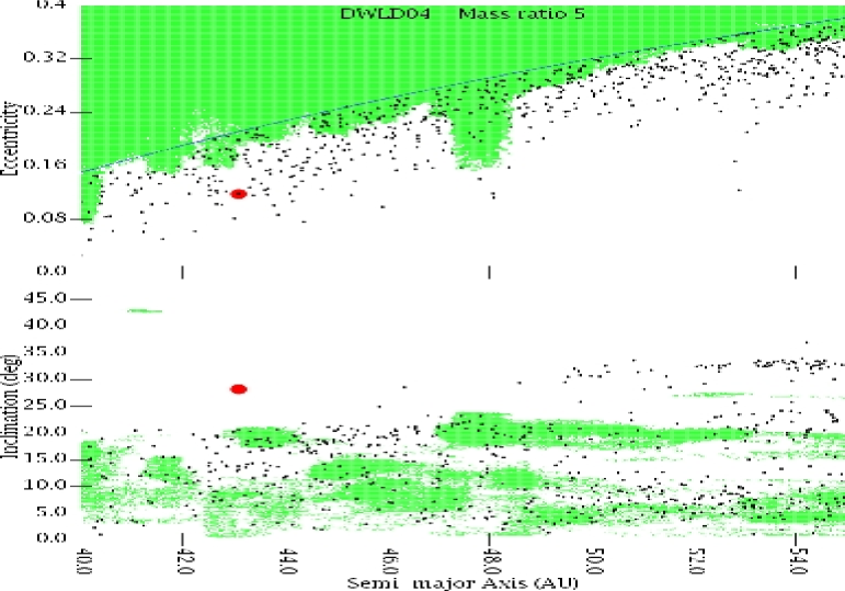
Figure 2: The green area illustrates the regions (eccentricity — semi-major axis distribution on the top panels and inclination — semi-major axis distribution on the bottom panels) visited by scattered disk objects with no collisions included (left panels: from LD/DL97; right panels: from DWLD04; bottom TGML05). The blue curve in the top panels marks $q\!=\!34\,$AU and the red dot shows the center of mass orbit of the EL₆₁ family (RB07). The minimum difference in orbital velocity between the EL₆₁ family and the scattered disk visited region is $265\,$m/s. For reference, a typical impact of scattered disk bodies with a mass ratio of 5 (as for the target/impactor estimated in BBRS) gives a $\delta V_{\rm min}$ of $\sim 450$ m/s. The black dots show stable Kuiper belt orbits that result from actual simulations of SD evolution, accounting for such collisions. In all cases the osculating orbits are shown.

The distance in velocity space between the location of the family and the scattered disk region, $\Delta V_{\rm min}$, can be computed using the techniques developed in Nesvorný et al. (2007b). Given two crossing orbits this algorithm uses Gauss’ equations to seek the minimum relative velocity ($\Delta V$) needed to move an object from one orbit to another. In particular, it searches through all values of true longitudes and orbital orientations in space to find the smallest $\Delta V$ while holding $a$, $e$, and $i$ of each orbit fixed. Using this algorithm, we take each entry from the orbital distributions saved during the scattered disk $N$-body simulations and compare it to RB07’s center of mass orbit for the EL₆₁ family. We then take $\Delta V_{\rm min}$ to be the minimum difference in orbital velocity between the EL₆₁ family and the region visited by scattered disk particles during our simulations. These values are listed in Table 2, and we find that all the $N$-body simulations have particles which get within $265\,$m/s of the family.

Next we estimate $\delta V_{\rm min}$. The center of mass velocity, $\vec{V}_{\rm CM}$, of target-impactor system is $(m_{i}\vec{V}_{i}+m_{t}\vec{V}_{t})/(m_{i}+m_{t})$, where $m$ is the mass of each body. So, $\delta V\equiv|\vec{V}_{\rm CM}-\vec{V}_{t}|=|\vec{V}_{i}-\vec{V}_{t}|/(1+\frac{m_{t}}{m_{i}})$, where $|\vec{V}_{i}-\vec{V}_{t}|$ is the impact speed, which BBRS argues is roughly $3\,$km/s (in the simulations below we find the average to be about $2.7\,$km/s). Therefore, assuming a mass ratio between the target and impactor of 5 (as argued by BBRS), we expect that the center of mass velocity (from which the fragments are ejected) to be offset from the initial velocity of the target by about $450\,$m/s. Since this is larger than the minimum velocity distance that separates the scattered disk from the EL₆₁ family ($\Delta V_{\rm min}$; $<\!265\,$m/s, as discussed above), it is possible that the observed orbit of the EL₆₁ family could result from such a collision.

We now estimate the likelihood that such a collision will happen. To accomplish this, we divide the problem into two parts. We first evaluate the probability ($p_{ss}$) that a collision occurred in the age of the Solar System between two SDOs with $R_{i}\!=\!500\,$km and $R_{t}\!=\!850\,$km. Then, we calculate the likelihood ($p_{KB}$) that the center of mass of the two colliding bodies was on a stable Kuiper belt orbit. Since fragments of the collision will be centered on this orbit, the family members should span it. In what follows, we refer to this theoretical orbit as the ‘collision orbit’. The probability that the EL₆₁ family originated in the scattered disk is thus $p_{SD}=p_{ss}\times p_{KB}$.

As with the determination of $p_{sk}$ in §2.2, we need to modify Eq. 1 to take into account that the number of objects in the scattered disk is changing with time. In this case, however, both the number of targets and the number of impactors vary. As result,

$$p_{ss}=(R_{i}+R_{t})^{2}\,\bar{\varrho}_{ss}\,\int{N_{i}(t)\,N_{t}(t)\,dt}.$$ (5)

Assuming that the size distribution of SDOs does not change with time, $N_{t}(t)/N_{t0}=N_{i}(t)/N_{i0}=f(t)$, where $f(t)$ was defined above. Thus, $\int{N_{i}(t)\,N_{t}(t)\,dt}$ becomes $N_{i0}N_{t0}\int{f^{2}\,dt}$. Now, if we define $t_{l}\equiv\int{f^{2}dt}$, then $p_{ss}$ again takes on the same form as in Eq. 1:

$$p_{ss}=N_{i0}\,N_{t0}\,t_{l}\,(R_{i}+R_{t})^{2}\,\bar{\varrho}_{ss},$$ (6)

where the subscript $ss$ refers to the fact that we are calculating these values for SDO—SDO collisions. Note that $t_{l}$ is not the same as $\bar{t}$ used in Eq. 3, but it is a measure of the characteristic time of the collision. The values of $t_{l}$ for our three scattered disk models are given in Table 2.

The values of $N_{i0}$ are the same as we calculated in §2.2 using Eq. 4 because in both cases the impacting population is the same. In this case, we can also use Eq. 4 to estimate $N_{t0}$. These values are given in Table 2. The table also shows the values of $\bar{\varrho}_{ss}$ for each of the models, which were again calculated using the Bottke et al. (1994) algorithm. Recall that this parameter only depends on the orbital element distribution of the scattered disk.

We can now evaluate $p_{ss}$ for the various models. These too are given in Table 2. Again, we are assuming a target radius of $850\,$km and a impactor radius of $500\,$km. We find that our scenario is least likely in the LD/DL97 model, with $p_{ss}\lesssim 0.06$, while it is most likely in the TGML05 model with $p_{ss}\!\sim\!1$. The fact that $p_{ss}$ can be close to one is encouraging. After all, we see one family and there are probably not many more in this size range. However, we urge caution in interpreting these $p_{ss}$ values because there are significant uncertainties in several of the numbers used to calculate them — particularly the $N$’s. Indeed, we believe that the differences between the $p_{ss}$ values from the various models are probably more a result of the intrinsic uncertainties in our procedures rather than the merit of one model over another.

Next, we need to calculate the probability that the impacts described above have collision orbits in the Kuiper belt ($p_{KB}$). We accomplish this with the use of a Monte Carlo simulation where we take the output of our three orbital integrations and randomly choose particle pairs to collide with one another based on their location and the local number density. We apply the following procedures to the LD/DL97, DWLD04, and TGML05 datasets, separately.

Our preexisting $N$-body simulations supply us with a series of snapshots of the evolving scattered disk as a function of time. In particular, the original $N$-body code recorded the position and velocity of each object in the system at fixed time intervals. For two objects to collide, they must be at the same place at the same time. However, because of the small number of particles in our simulations (compared to the real scattered disk) and the fact that the time intervals between snapshots are long, it is very unlikely to find any actual collisions in our list of snapshots. Thus, we must bin our data in both space and time in order to generate pairs of particles to collide. For this purpose, we divided the Solar System into a spatial grid. We assumed that the spatial distribution of particles is both axisymmetric and symmetric about the mid-plane. Thus, our grid covers the upper part of the meridional plane. The cylindrical radius ($\varpi$) was divided into 300 bins between 30 and $930\,$AU, while the positive part of the vertical coordinate was divided into 100 bins with $z\!\leq\!100\,$AU. We also binned time. However, since the number of particles in the $N$-body simulations decreases with time (see Figure 1), we increased the width of the time bins ($\Delta t_{\rm bin}$) at later times in order to insure we had enough particles in each bin to collide with one another. In particular, we choose the width of each time bin so that the total number of particles in the bin (summing over the spatial bins) is the same.

We assigned each entry (meaning a particular particle at a particular time) in the dataset of our original $N$-body simulation to a bin in the 3-dimensional space discussed above (i.e. $\varpi$–$z$–$t$). As a result, the entries associated with each bin represent a list of objects that were roughly at the same location at roughly the same time in the $N$-body simulation.

Finally, we generated collisions at random. This was accomplished by first randomly choosing a bin based on the local collision rate, as determined by a particle-in-the-box calculation. It is important to note that since the bins were populated using the $N$-body simulations, this choice is consistent with the collision rates used to calculate the mean collision probability $p_{ss}$ above. As a result, we are justified multiplying $p_{ss}$ and $p_{KB}$ together at the end of this process. Once we had chosen a bin, we randomly chose a target and impactor from the list of objects in that bin. From the velocities of the colliding pair we determined the orbit of the pair’s center-of-mass assuming a mass ratio of 5.

The next issue is to determine whether these collision orbits are in the Kuiper belt. For this purpose, we define a KBO as an object on a stable (for at least a long period of time) orbit with a perihelion distance, $q$, greater than $34\,$AU (indicated by the blue curves in Figure 2). To test stability, we performed a $50\,$Myr integration of the orbit under the gravitational influence of the Sun and the four giant planets. As previous studies of the stability of KBOs have shown (Duncan et al. 1995; Kuchner et al. 2002), a time-span of $50\,$Myr adequately separates the stable from the unstable regions of the Kuiper belt. Any object that evolved onto an orbit with $q\!<\!33\,$AU during this period of time was assumed to be unstable. The remainder were assumed to be stable and are shown as the black dots in Figure 2.

We find that collisions can effectively fill the Kuiper belt out to near Neptune’s 1:2 mean motion resonance at $48\,$AU. We created stable, non-resonant objects with $q$’s as large as $46.5\,$AU. Indeed, the object with the largest $q$ has $a\!=\!47.3\,$AU, $e\!=\!0.017$, and $i\!=\!18.2^{\circ}$ and thus it is fairly typical of the KBOs that we see. With regard to the EL₆₁ family, we easily reproduce stable orbits with the same $a$ and $e$. However, we find that it is difficult to reproduce the family’s inclination. Although we do produce a few orbits with inclinations larger than the family’s, $\sim\!90\%$ of the orbits in our simulations have inclinations less than that of the EL₆₁ family.

The lack of high inclination objects is clearly a limitation of our model. We believe, however, that this mismatch is more the result of limitations in our scattered disk models than of our collisional mechanism for capture in the Kuiper belt. Neither the LD/DL97, DWLD04, nor TGML05 simulations produce high enough inclinations to explain what we see in the scattered disk. So, if we had a more realistic scattered disk model, we would probably be able to produce more objects with inclinations like EL₆₁ and it cohorts. One concern of such a solution is that the higher inclinations would affect our collision probabilities, particularly through their effects on $\varrho_{ss}$. To check this, we performed a new set of calculations where we arbitrarily increased the inclinations of the scattered disk particles by a factor of 2. We find that the increased inclinations decrease $\varrho_{ss}$ by less than 20%. Thus, we conclude that if we had access to a scattered disk model with more realistic inclinations, we should be able to better reproduce the orbit of the family without significantly affecting the probability of producing it.

The values of $p_{\rm KB}$ (the fraction of EL₆₁-forming impacts that lead to objects that are trapped in the Kuiper belt) resulting from our main Monte Carlo simulations are listed in Table 2. Combining $p_{\rm KB}$ and $p_{ss}$ we find that the probability that, in the age of the Solar System, two SDOs with radii of $500\,$km and $850\,$km hit one another leading to a family in the Kuiper belt (which we called $p_{\rm SD}$) is between 0.1% and 47%, depending on the assumptions we use. For comparison, in §2 we computed that the probability that the EL₆₁ family is the result of the collision between two Kuiper belt objects is $\sim\!0.02\%$, or is the result of a KBO–SDO collision is $\lesssim\!0.1\%$. Thus, we conclude that the progenitors of the EL₆₁ family are much more likely to have originated in the scattered disk than in the Kuiper belt.

Up to this point, we have been concentrating on whether our model can reproduce the observed center of mass orbit of the EL₆₁ family. However, the spread of orbits could also represent an important observational constraint (Morbidelli et al. 1995). In particular, assuming that the ejection velocities of the collision were isotropic around the center of mass, the family members should fall inside an ellipse in $a$–$e$ and $a$–$i$ space. The orientation and axis ratio of the ellipse in $a$–$e$ space are strong functions of the mean anomaly of the collision orbit at the time of the impact ($M$), while the axis ratio of the ellipse in $a$–$i$ space is a function of both $M$ and the argument of perihelion ($\omega$). The major axis of the ellipse in $a$–$i$ space should always be parallel to the $a$ axis. Using this information, RB07 estimated that at the time of the collision, the center of mass orbit had $M\!=\!76^{\circ}$ and $\omega\!=\!271^{\circ}$.

Given that we are arguing that the target and impactor originated in the scattered disk, we might expect that certain impact geometries are preferred, while others are forbidden. Thus, we examined the $M$ and $\omega$ of all the collisions shown in Figure 2 (black dots) with orbits near that of RB07’s center-of-mass orbit. In particular, we chose collision orbits with $42\!<\!a\!<\!44\,$AU, $0.08\!<\!e\!<\!0.14$, and $i\!>\!15^{\circ}$. We found that we cannot constrain the values of $\omega$. Indeed, these orbits are roughly uniform in this angle. However, our model avoids values of $M$ between $-37^{\circ}$ and $62^{\circ}$, i.e. near perihelion. This is a result of the fact that the collision must conserve momentum, lose energy, and that the initial orbits of the progenitors were in the scattered disk while the family must end up in the Kuiper belt. RB07’s value of $M$ falls in the range covered by our models.

Figure 3 shows a comparison between the spread of the EL₆₁ family in orbital element space (black dots) and two of our fictitious families. The fictitious family members were generated by isotropically ejecting particles from the point of impact with a velocity of 150 m/s (BBRS). The collision orbits for these families are consistent with the center of mass orbit for the family. The collision orbit of the family shown in green has $M\!=\!71^{\circ}$ and $\omega\!=\!273^{\circ}$ — similar to the values inferred by RB07. For comparison, the family shown in red has an orbit with similar $a$, $e$, and $i$, but $M\!=\!174^{\circ}$ and $\omega\!=\!294^{\circ}$. We can conclude that, although this test is not very constraining because our model can reproduce most values and $M$ and $\omega$, we can match what is seen.

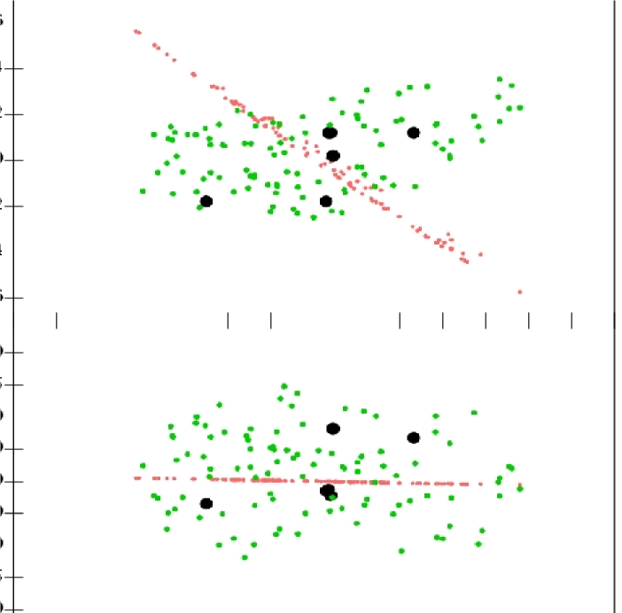
Figure 3: A comparison of the spread of families in $\Delta a$–$\Delta e$ and $\Delta a$–$\Delta i$ space, where $\Delta x$ is defined to be the difference between a particular orbital element of the family member and that of the collision orbit. The black dots show the proper orbital elements of the real family members as determined by RB07. We did not plot 2003 EL₆₁ or 1999 OY₃ because their orbits have changed since the family formed (RB07). The green dots show a fictitious family with a collision orbit of $a\!=\!42.0\,$AU, $e\!=\!0.09$, $i\!=\!21^{\circ}$, $\omega\!=\!111^{\circ}$, $M\!=\!-72^{\circ}$. For comparison, the red dots show a fictitious family with a collision orbit of $a\!=\!42.2\,$AU, $e\!=\!0.09$, $i\!=\!23^{\circ}$, $\omega\!=\!294^{\circ}$, $M\!=\!174^{\circ}$. This shows that this diagnostic is a sensitive test for the models and that we can reproduce the observations.

There is one more issue we must consider. In §2.1, we described the three phases of Kuiper belt evolution: 1) A quiescent phase of growth (Stage I), 2) a violent phase of dynamical excitation and, perhaps, mass depletion (Stage II), and 3) a relatively benign modern phase (Stage III). We argued that any collisional family that formed during Stage I or Stage II would have been dispersed during the chaotic events that excited the orbits in the Kuiper belt. Thus, the family forming impact must have occurred during Stage III. However, the fact that the violent evolution is over before the collision does not mean that the orbits of the planets must have remained unchanged. As a matter of fact, the decay of the scattered disk population actually causes Neptune’s orbit to slowly migrate outward. This, in turn, causes resonances to sweep through the Kuiper belt, potentially affecting the orbits of some KBOs. So, as a final step in our analysis, we must determine whether the dynamical coherence of the EL₆₁ family would be preserved during this migration.

To address the above issue, we performed an integration of 100 fictitious family members on orbits initially with the same $a$, $e$, and $i$ as RB07’s center of mass orbit, under the gravitational influence of the four giant planets as they migrate. We adopted the case presented in Malhotra (1995), where Neptune migrated from 23 to $30\,$AU. Note that the model in Levison et al. (2008) has Neptune migrating from $\sim\!27\,$AU, so we are adopting an extreme range of migration here. We found that only 12% of the family members were trapped in and pushed outward by Neptune’s mean motion resonances (i.e. they were removed from the family). The orbits of the remaining particles were only slightly perturbed and thus they remained recognizable family members. Thus, we conclude that the family would have survived the migration and that the SDO-SDO collision is still a valid model for the origins of the EL₆₁ family. Interestingly, however, this simulation predicts that we might find family members (which can be identified by their IR spectra; BBRS) in the more distant Neptune resonances (1:2, 2:5…). If so, the location of these objects can be used to constrain Neptune location at the time when the EL₆₁ family formed.

So, we conclude that the most probable scenario for the origin of the EL₆₁ family is that it resulted from a collision between two SDOs. If true, this result has implications far beyond the origin of a single collisional family because it shows, for the first time, that collisions can affect the dynamical evolution of the Kuiper belt, in particular, and small body populations, in general. Indeed, this process might be especially important for the so-called ‘hot’ classical Kuiper belt. Brown (2001) argued that the de-biased inclination distribution of the classical Kuiper belt is bi-modal and can be fitted with two Gaussian functions, one with a standard deviation $\sigma\sim 2^{\circ}$ (the low-inclination ‘cold’ core), and the other with $\sigma\sim 12^{\circ}$ (the high-inclination ‘hot’ population). Since the work of Brown, it has been shown that the members of these two populations have different physical properties (Tegler & Romanishin 2000; Levison & Stern 2001; Doressoundiram et al. 2001), implying different origins.

Gomes (2003) suggested that one way to explain the differences between the hot and cold populations is that the hot population originated in the scattered disk, because a small fraction of the scattered disk could be captured into the Kuiper belt due to the gravitational effects of planets as they migrated. Here we show that collisions can accomplish the same result. Indeed, a collisional origin for these objects may have the advantage of explaining why binaries with equal mass-components are rarer in this population than in other parts of the trans-Neptunian region. Using HST, Noll et al. (2008) found that 29% of classical Kuiper belt objects (see their paper for a precise definition) with inclination $<\!5.5^{\circ}$ are similar-mass binary objects, while this fraction is only 2% for objects with larger inclinations. A collisional origin for the hot population might explain this discrepancy because a collision that is violent enough to kick an object from the scattered disk to the Kuiper belt would also disrupt the binary (the binary member that was not struck would have continued in the scattered disk).

One might expect that if the majority of the hot population was put in place by collisions, we should be able to predict a relationship between the size distribution of its members and that of the scattered disk. Eq. 6 shows that the collision probability scales roughly as $N^{2}$. And since in the scattered disk, $N(R)\propto R^{-q}$, we might predict that the size distribution of the hot population is $N_{h}(R)\propto R^{2-2q}$ (one power of $-q$ from both $N_{i0}$ and $N_{0t}$, and a power of 2 from $(R_{i}+R_{t})^{2}$, see Eq. 6). In this case $q\!\sim\!3$ (see above) and thus $N_{h}(R)\sim R^{-4}$. However, this estimate does not take into account the fact that the collisions themselves could affect the size distribution of the resulting hot population. Unfortunately, it is not yet clear what the size of the fragments would be because of poor understanding of the collisional physics of icy objects at these energies. As a result, it is not yet possible to investigate this intriguing idea.

4 Conclusions

The recent discovery of the EL₆₁ family in the Kuiper belt (BBRS) is surprising because its formation is, at first glance, a highly improbable event. BBRS argues that this family is the result of a collision between two objects with radii of $\sim\!850\,$km and $\sim\!500\,$km. The chances that such event would have occurred in the current Kuiper belt in the age of the Solar System is roughly 1 in $4000$ (see §2). In addition, it is not possible for the collision to have occurred in a massive primordial Kuiper belt because the dynamical coherence of the family would not have survived whatever event molded the final Kuiper belt structure. We also investigated the idea that the family could be the result of a target KBO being struck by a SDO projectile, and found that the probability of such an event forming a family on a stable Kuiper belt orbit is $\lesssim\!10^{-3}$.

In this paper, we argue that the EL₆₁ family is the result of a collision between two scattered disk objects. In particular, we present the novel idea that the collision between two SDOs on highly eccentric unstable orbits could damp enough orbital energy so that the family members would end up on stable Kuiper belt orbits. This idea of using the scattered disk as the source of both of the family’s progenitors has the advantage of significantly increasing the probability of a collision because the population of the scattered disk was much larger in the early Solar System (it is currently eroding away due to the gravitational influence of Neptune — DL97; DWLD04). With the use of three pre-existing models of the dynamical evolution of the scattered disk (DWLD04, LD/DL97, and TGML05) we show that the probability that a collision between a $\sim\!850\,$km SDO and $\sim\!500\,$km SDO occurred and that the resulting collisional family was spread around a stable Kuiper belt orbit can be as large as 47%. Given the uncertainties involved, this can be considered on the order of unity. Thus, we conclude that the EL₆₁ family progenitors are significantly more likely to have originated in the scattered disk than the Kuiper belt.

If true, this result has important implications for the origin of the Kuiper belt because it is the first direct indication that collisions can affect the dynamical evolution of this region. Indeed, we suggest at the end of §3 that this process might be responsible for the emplacement of the so-called ‘hot’ classical belt (Brown 2001) because it naturally explains why so few of these objects are found to be binaries (Noll et al. 2008).

References

• Benz, W., Asphaug, E. 1999. Catastrophic Disruptions Revisited. Icarus 142, 5-20.

• Bernstein, G. M., Trilling, D. E., Allen, R. L., Brown, M. E., Holman, M., Malhotra, R. 2004. The Size Distribution of Trans-Neptunian Bodies. Astronomical Journal 128, 1364-1390.

• Bottke, W. F., Nolan, M. C., Greenberg, R., Kolvoord, R. A. 1994. Velocity distributions among colliding asteroids. Icarus 107, 255-268.

• Brown, M. E. 2001. The Inclination Distribution of the Kuiper Belt. Astronomical Journal 121, 2804-2814.

• Brown, M. E., and 14 colleagues 2005. Keck Observatory Laser Guide Star Adaptive Optics Discovery and Characterization of a Satellite to the Large Kuiper Belt Object 2003 EL₆₁. Astrophysical Journal 632, L45-L48.

• Brown, M. E., Schaller, E. L. 2007. The Mass of Dwarf Planet Eris. Science 316, 1585.

• Brown, M. E., Trujillo, C. A., Rabinowitz, D. L. 2005. Discovery of a Planetary-sized Object in the Scattered Kuiper Belt. Astrophysical Journal 635, L97-L100.

• Brown, M. E., Barkume, K. M., Ragozzine, D., Schaller, E. L. 2007. A Collisional Family of Icy Objects in the Kuiper Belt. Nature 446, 294-296.

• Canup, R. M. 2005. A Giant Impact Origin of Pluto-Charon. Science 307, 546-550.

• Davis, D. R., Farinella, P. 1997. Collisional Evolution of Edgeworth-Kuiper Belt Objects. Icarus 125, 50-60.

• Dones, L., Weissman, P. R., Levison, H. F., Duncan, M. J. 2004. Oort cloud formation and dynamics. Comets II 153-174.

• Doressoundiram, A., Barucci, M. A., Romon, J., Veillet, C. 2001. Multicolor Photometry of Trans-neptunian Objects. Icarus 154, 277-286.

• Duncan, M. J., Levison, H. F. 1997. A scattered comet disk and the origin of Jupiter family comets. Science 276, 1670-1672.

• Duncan, M. J., Levison, H. F., Budd, S. M. 1995. The Dynamical Structure of the Kuiper Belt. Astronomical Journal 110, 3073-3081.

• Duncan, M., Levison, H., Dones, L. 2004. Dynamical evolution of ecliptic comets. Comets II 193-204.

• Gladman, B., Kavelaars, J. J., Petit, J.-M., Morbidelli, A., Holman, M. J., Loredo, T. 2001. The Structure of the Kuiper Belt: Size Distribution and Radial Extent. Astronomical Journal 122, 1051-1066.

• Gomes, R. S. 2003. The origin of the Kuiper Belt high-inclination population. Icarus 161, 404-418.

• Gomes, R., Levison, H. F., Tsiganis, K., Morbidelli, A. 2005. Origin of the cataclysmic Late Heavy Bombardment period of the terrestrial planets. Nature 435, 466-469.

• Gomes, R. S., Fernández, J., Gallardo, T., Brunini, A. 2007. The Scattered Disk: Origins, Dynamics and End States. The Solar System Beyond Neptune. 259-273.

• Hahn, J. M., Malhotra, R. 2005. Neptune’s Migration into a Stirred-Up Kuiper Belt: A Detailed Comparison of Simulations to Observations. Astronomical Journal 130, 2392-2414.

• Kenyon, S. J., Luu, J. X. 1998. Accretion in the Early Kuiper Belt. I. Coagulation and Velocity Evolution. Astronomical Journal 115, 2136-2160.

• Kenyon, S. J., Luu, J. X. 1999. Accretion in the Early Outer Solar System. Astrophysical Journal 526, 465-470.

• Kenyon, S. J., Bromley, B. C. 2002. Collisional Cascades in Planetesimal Disks. I. Stellar Flybys. Astronomical Journal 123, 1757-1775.

• Kenyon, S. J., Bromley, B. C. 2004. The Size Distribution of Kuiper Belt Objects. Astronomical Journal 128, 1916-1926.

• Kenyon, S. J., Bromley, B. C., O’Brien, D. P., Davis, D. R. 2008. Formation and Collisional Evolution of Kuiper belt Objects. The Solar System Beyond Neptune 293-314.

• Kuchner, M. J., Brown, M. E., Holman, M. 2002. Long-Term Dynamics and the Orbital Inclinations of the Classical Kuiper Belt Objects. Astronomical Journal 124, 1221-1230.

• Levison, H. F., Duncan, M. J. 1994. The long-term dynamical behavior of short-period comets. Icarus 108, 18-36.

• Levison, H. F., Duncan, M. J. 1997. From the Kuiper Belt to Jupiter-Family Comets: The Spatial Distribution of Ecliptic Comets. Icarus 127, 13-32.

• Levison, H. F., Stern, S. A. 2001. On the Size Dependence of the Inclination Distribution of the Main Kuiper Belt. Astronomical Journal 121, 1730-173

• Levison, H. F., Morbidelli, A., Van Laerhoven, C., Gomes, R., Tsiganis, K.  2008. Origin of the structure of the Kuiper Belt during a Dynamical Instability in the Orbits of Uranus and Neptune. Icarus 196, 258-273.

• Malhotra, R. 1995. The Origin of Pluto’s Orbit: Implications for the Solar System Beyond Neptune. Astronomical Journal 110, 420.

• Morbidelli, A. 2007. Solar system: Portrait of a suburban family. Nature 446, 273-274.

• Morbidelli, A., Zappala, V., Moons, M., Cellino, A., Gonczi, R. 1995. Asteroid families close to mean motion resonances: dynamical effects and physical implications. Icarus 118, 132.

• Morbidelli, A., Valsecchi, G. B. 1997. NOTE: Neptune Scattered Planetesimals Could Have Sculpted the Primordial Edgeworth-Kuiper Belt. Icarus 128, 464-468.

• Morbidelli, A., Emel’yanenko, V. V., Levison, H. F. 2004. Origin and orbital distribution of the trans-Neptunian scattered disc. Monthly Notices of the Royal Astronomical Society 355, 935-940.

• Morbidelli, A., Levison, H. F., Tsiganis, K., Gomes, R. 2005. Chaotic capture of Jupiter’s Trojan asteroids in the early Solar System. Nature 435, 462-465.

• Morbidelli, A., Levison, H. F., Gomes, R. 2007. The Dynamical Structure of the Kuiper Belt and its Primordial Origin. The Kuiper Belt, in press.

• Nagasawa, M., Ida, S. 2000. Sweeping Secular Resonances in the Kuiper Belt Caused by Depletion of the Solar Nebula. Astronomical Journal 120, 3311-3322.

• Nesvorný, D., Vokrouhlický, D., Morbidelli, A. 2007a. Capture of Irregular Satellites during Planetary Encounters. Astronomical Journal 133, 1962-1976.

• Nesvorný, D., Vokrouhlický, D., Bottke, W. F., Gladman, B., Häggström, T. 2007b. Express delivery of fossil meteorites from the inner asteroid belt to Sweden. Icarus 188, 400-413.

• Noll, K. S., Grundy, W. M., Stephens, D. C., Levison, H. F., Kern, S. D. 2008. Evidence for two populations of classical transneptunian objects: The strong inclination dependence of classical binaries. Icarus 194, 758-768.

• Petit, J.-M., Holman, M. J., Gladman, B. J., Kavelaars, J. J., Scholl, H., Loredo, T. J. 2006. The Kuiper Belt luminosity function from $m_{R}=$ 22 to 25. Monthly Notices of the Royal Astronomical Society 365, 429-438.

• Rabinowitz, D. L., Barkume, K., Brown, M. E., Roe, H., Schwartz, M., Tourtellotte, S., Trujillo, C. 2006. Photometric Observations Constraining the Size, Shape, and Albedo of 2003 EL61, a Rapidly Rotating, Pluto-sized Object in the Kuiper Belt. Astrophysical Journal 639, 1238-1251.

• Ragozzine, D., Brown, M. E. 2007. Candidate Members and Age Estimate of the Family of Kuiper Belt Object 2003 EL61. Astronomical Journal 134, 2160-2167.

• Sheppard, S. S., Trujillo, C. A. 2006. A Thick Cloud of Neptune Trojans and Their Colors. Science 313, 511-514.

• Stern, S. A. 1996. On the Collisional Environment, Accretion Time Scales, and Architecture of the Massive, Primordial Kuiper Belt.. Astronomical Journal 112, 1203.

• Stern, S. A., Colwell, J. E. 1997a. Accretion in the Edgeworth-Kuiper Belt: Forming 100-1000 KM Radius Bodies at 30 AU and Beyond. Astronomical Journal 114, 841.

• Stern, S. A., Colwell, J. E. 1997b. Collisional Erosion in the Primordial Edgeworth-Kuiper Belt and the Generation of the 30-50 AU Kuiper Gap. Astrophysical Journal 490, 879.

• Tegler, S. C., Romanishin, W. 2000. Extremely red Kuiper-belt objects in near-circular orbits beyond 40 AU. Nature 407, 979-981.

• Thommes, E. W., Duncan, M. J., Levison, H. F. 1999. The formation of Uranus and Neptune in the Jupiter-Saturn region of the Solar System. Nature 402, 635-638.

• Thommes, E. W., Duncan, M. J., Levison, H. F. 2002. The Formation of Uranus and Neptune among Jupiter and Saturn. Astronomical Journal 123, 2862-2883.

• Trujillo, C. A., Jewitt, D. C., Luu, J. X. 2000. Population of the Scattered Kuiper Belt. Astrophysical Journal 529, L103-L106.

• Tsiganis, K., Gomes, R., Morbidelli, A., Levison, H. F. 2005. Origin of the orbital architecture of the giant planets of the Solar System. Nature 435, 459-461.