From Data to the p-Adic or Ultrametric Model

Abstract

We model anomaly and change in data by embedding the data in an ultrametric space. Taking our initial data as cross-tabulation counts (or other input data formats), Correspondence Analysis allows us to endow the information space with a Euclidean metric. We then model anomaly or change by an induced ultrametric. The induced ultrametric that we are particularly interested in takes a sequential – e.g. temporal – ordering of the data into account. We apply this work to the flow of narrative expressed in the film script of the Casablanca movie; and to the evolution between 1988 and 2004 of the Colombian social conflict and violence.

1 Modeling of Anomaly or Change: Introduction

The data mining and data analysis challenges addressed are the following. (i) Great masses of data, textual and otherwise, need to be exploited and decisions need to be made. Correspondence Analysis handles multivariate numerical and symbolic data with ease. (ii) Structures and interrelationships evolve in time. (iii) We must consider a complex web of relationships. (iv) We need to address all these issues from data sets and data flows.

Various aspects of how we respond to these challenges will be discussed in this article, complemented by the Appendix. We will look at how this works, using the Casablanca film script, and data from the long Colombian civil strife involving government, guerrillas, paramilitaries and civilians.

2 The Geometry and Topology of Information

We consider Correspondence Analysis and hierarchical clustering as a semantic analysis platform. To illustrate our description, we will take film script, the semi-structured expression of a story. Film script is the starting point of what may become a movie.

For McKee [4], film script text is the “sensory surface of a work of art” and reflects the underlying emotion or perception. Our data mining approach models and tracks these underlying aspects in the data. Our approach to textual data mining has a range of novel elements.

The starting point for analysis is frequency of occurrence data, typically the ordered scenes crossed by all words used in the script.

If the totality of interrelationships is one facet of semantics, then another is anomaly (or change, novelty, breakpoint) as modeled by a clustering hierarchy. If, therefore, a scene is quite different from immediately previous scenes, then it will be incorporated into the hierarchy at a high level. This novel view of hierarchy will be discussed further in section 2.1 below.

We draw on these two vantage points on semantics – viz. totality of interrelationships, and using a hierarchy to express change. See [1] for other work that uses p-adic metric properties, tantamount to ultrametric properties, for the same goal of change detection.

2.1 Modeling Semantics via the Geometry and Topology of Information

Some underlying principles are as follows. We start with the cross-tabulation data, scenes $\times$ attributes. Scenes and attributes are embedded in a metric space. This is how we are probing the geometry of information, which is a term and viewpoint used by [13].

Underpinning the display in Figure 3 is a Euclidean embedding. The triangular inequality holds for metrics. An example of a metric is the Euclidean distance, exemplified in Figure 1, where each and every triplet of points satisfies the relationship: $d(x,z)\leq d(x,y)+d(y,z)$ for distance $d$. Two other relationships also must hold. These are symmetry and positive definiteness, respectively: $d(x,y)=d(y,x)$, and $d(x,y)>0$ if $x\neq y$, $d(x,y)=0$ if $x=y$.

Figure 1: The triangular inequality defines a metric: every triplet of points satisfies the relationship: $d(x,z)\leq d(x,y)+d(y,z)$ for distance $d$.

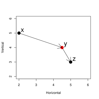
Further underlying principles used in Figure 3 are as follows. The axes are the principal axes of momentum. Identical principles are used as in classical mechanics. The scenes are located as weighted averages of all associated attributes; and vice versa.

Huyghens’ theorem relates to decomposition of inertia of a cloud of points. This is the basis of Correspondence Analysis.

We come now to a different principle: that of the topology of information. The particular topology used is that of hierarchy. Euclidean embedding provides a very good starting point to look at hierarchical relationships. An innovation in our work is as follows: the hierarchy takes sequence, e.g. timeline, into account. This captures, in a more easily understood way, the notions of novelty, anomaly or change.

Let us take an informal case study to see how this works. Consider the situation of seeking documents based on titles. If the target population has at least one document that is close to the query, then this is (let us assume) clearcut. However if all documents in the target population are very unlike the query, does it make any sense to choose the closest? Whatever the answer here we are focusing on the inherent ambiguity, which we will note or record in an appropriate way. Figure 2, left, illustrates this situation where the query is the point to the right.

Figure 2: Left: The query is on the far right. While we can easily determine the closest target (among the three objects represented by the dots on the left), is the closest really that much different from the alternatives? Right: The strong triangular inequality defines an ultrametric: every triplet of points satisfies the relationship: $d(x,z)\leq\mbox{max}\{d(x,y),d(y,z)\}$ for distance $d$. Cf. by reading off the hierarchy, how this is verified for all $x,y,z$: $d(x,z)=3.5;d(x,y)=3.5;d(y,z)=1.0$. In addition the symmetry and positive definiteness conditions hold for any pair of points.

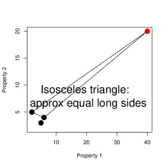
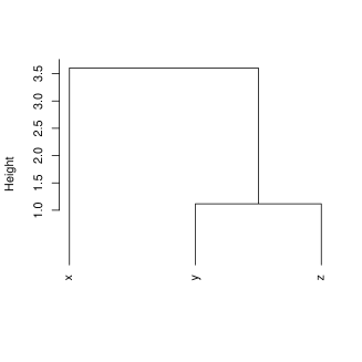
By using approximate similarity this situation can be modeled as an isosceles triangle with small base, as illustrated in Figure 2, left. An ultrametric space has properties that are very unlike a metric space, and one such property is that the only triangles allowed are either (i) equilateral, or (ii) isosceles with small base. So Figure 2 can be taken as representing a case of ultrametricity. What this means is that the query can be viewed as having a particular sort of dominance or hierarchical relationship vis-à-vis any pair of target documents. Hence any triplet of points here, one of which is the query (defining the apex of the isosceles, with small base, triangle), defines local hierarchical or ultrametric structure. (See [6] for case studies.)

It is clear from Figure 2 that we should use approximate equality of the long sides of the triangle. The further away the query is from the other data then the better is this approximation [6].

What sort of explanation does this provide for our conundrum? It means that the query is a novel, or anomalous, or unusual “document”. It is up to us to decide how to treat such new, innovative cases. It raises though the interesting perspective that here we have a way to model and subsequently handle the semantics of anomaly or innocuousness.

3 The Changing Nature of Movie and Drama

3.1 Background

McKee [4] bears out the great importance of the film script: “50% of what we understand comes from watching it being said.” And: “A screenplay waits for the camera. … Ninety percent of all verbal expression has no filmic equivalent.”

An episode of a television series costs US$ 2–3 million per one hour of television. Generally screenplays are written speculatively or commissioned, and then prototyped by the full production of a pilot episode. Increasingly, and especially availed of by the young, television series are delivered via the Internet. Originating in one medium – cinema, television, game, online – film and drama series are increasingly migrated to another. So scriptwriting must take account of digital multimedia platforms. This has been referred to in computer networking parlance as “multiplay” and in the television media sector as a “360 degree” environment.

Cross-platform delivery motivates interactivity in drama. So-called reality TV has a considerable degree of interactivity, as well as being largely unscripted.

There is a burgeoning need for us to be in a position to model the semantics of film script, – its most revealing structures, patterns and layers. With the drive towards interactivity, we also want to leverage this work towards more general scenario analysis. Other potential applications are to business strategy and planning; education and training; and science, technology and economic development policy.

3.2 Casablanca Narrative: Illustrative Analysis

The well known Casablanca movie serves as an example for us. Film scripts, such as for Casablanca, are partially structured texts. Each scene has metadata and the body of the scene contains dialog and possibly other descriptive data. The Casablanca script was half completed when production began in 1942. The dialog for some scenes was written while shooting was in progress. Casablanca was based on an unpublished 1940 screenplay [3]. It was scripted by J.J. Epstein, P.G. Epstein and H. Koch. The film was directed by M. Curtiz and produced by H.B. Wallis and J.L. Warner. It was shot by Warner Bros. between May and August 1942.

A data set was constructed from the 77 successive scenes crossed by attributes – Int[erior], Ext[erior], Day, Night, Rick, Ilsa, Renault, Strasser, Laszlo, Other (i.e. minor character), and 29 locations. Many locations were met with just once; Rick’s Café was the location of 36 scenes. In scenes based in Rick’s Café we did not distinguish between “Main room”, “Office”, “Balcony”, etc. Because of the plethora of scenes other than Rick’s Café we assimilate these to just one, “other than Rick’s Café”, scene.

In Figure 3, 12 attributes are displayed; 77 scenes are displayed as dots (to avoid over-crowding of labels). Approximately 34% (for factor 1) + 15% (for factor 2) = 49% of all information, expressed as inertia explained, is displayed here. We can study interrelationships between characters, other attributes, scenes, for instance closeness of Rick’s Café with Night and Int (obviously enough).

Figure 3: Correspondence Analysis of the Casablanca data derived from the script. The input data is presences/absences for 77 scenes crossed by 12 attributes. The 77 scenes are located at the dots, which are not labeled here for clarity. For a short review of the analysis methodology, see Appendix.

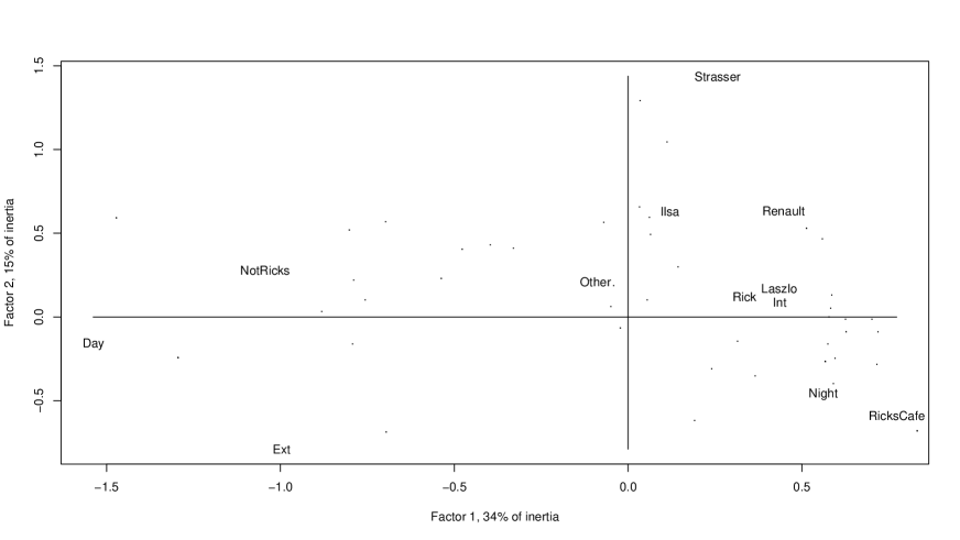
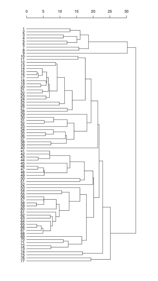
Figure 4 uses a sequence-constrained complete link agglomerative algorithm. It shows up scenes 9 to 10, and progressing from 39, to 40 and 41, as major changes. The sequence constrained algorithm, i.e. agglomerations are permitted between adjacent segments of scenes only, is described in an Appendix to this article, and in greater detail in [7]. The agglomerative criterion used, that is subject to this sequence constraint, is a complete link one.

A study in greater depth of the semantics of Casablanca can be found in [8]. We refer the reader to that work for further reading since, there, we use all words appearing in the screenplay rather than the set of 12 attributes that we limit ourselves to here.

Figure 4: 77 scenes clustered. These scenes are in sequence: a sequence-constrained agglomerative criterion is used for this. The agglomerative criterion itself is a complete link one. See [5] for properties of this algorithm.

3.3 Our Platform for Analysis of Semantics

Correspondence analysis supports the following: analysis of multivariate, mixed numerical/symbolic data; web of interrelationships; and evolution of relationships over time.

Correspondence Analysis is in practice a tale of three metrics [7]. The analysis is based on embedding a cloud of points from a space governed by one metric into another. Furthermore the cloud offers vantage points of both observables and their characterizations, so – in the case of film script – for any one of the metrics we can effortlessly pass between the space of film script scenes and attribute set. The three metrics are as follows.

• Chi squared, $\chi^{2}$, metric – appropriate for profiles of frequencies of occurrence.

• Euclidean metric, for visualization, and for static context.

• Ultrametric, for hierarchic relations and, as we use it in this work, for dynamic context.

In the analysis of semantics, we distinguish two separate aspects.

Firstly there is context – the collection of all interrelationships. The Euclidean distance makes a lot of sense when the population is homogeneous. All interrelationships together provide context, relativities – and hence meaning.

Secondly there is hierarchy which tracks anomaly. Ultrametric distance makes a lot of sense when the observables are heterogeneous, discontinuous. The latter is especially useful for determining anomalous (or atypical or innovative) cases.

4 Colombia Social Conflict: Analysis of Change

4.1 Background of the Data

The data used in this work related to social conflict and were produced by CERAC, the Conflict Analysis Resource Center, www.cerac.org.co. We will refer to the data used as the CERAC Colobmia Conflict database. It is being grown on an ongoing basis.

From [9], we use high frequency micro-data, relating to internal social conflict in Colombia (population: 44 million) from 1988 to 2004, hence over a period of 17 years. Social conflict is not ethnic, religious, nor regional, as often the case elsewhere, but is instead economical, political, and military, in origin. Economic factors, for instance, include the narcotics sector and kidnapping. A short periodization of the conflict is as follows [9]: 1988–1991, “adjustment period” due to the end of the Cold War; 1992–1996, “stagnation period”; and from 1997 onwards, “upsurge period”.

The CERAC data relates to actions, and their intensity, leading to information on impact. Armed combat is taken therefore as a clash, or an attack (relating, respectively, to bilateral or multilateral, versus unilateral, engagement). For the data period, the Colombian conflict has seen more than 3000 casualties per year. [10] discusses the effect of Alvaro Uribe becoming President in August 2002.

The study [11] underlines interest in civil war dynamics: “… We consider … different attack types (unopposed events) plus clashes … For each event type we determine the number of civilian killings and injuries … and the population density … We argue that policy must focus on … very specific circumstances for civilian casualties … [such as] massacres by illegal right-wing paramilitaries in rural areas — … These events account for almost 40% of all conflict casualties …”.

In this article, we study change versus continuity over time, allowing for gradation in such change. A hierarchical clustering is used, taking account of the timeline, furnishing a visualization of breakpoints and timeline resolution-related properties.

4.2 Correspondence Analysis and Metric Embedding

Starting with an array of counts of presence versus absence, or frequency of occurrence, which provides data that cross-tabulates a set of observations and a set of attributes, we can embed the observations and attributes in a Euclidean space. This factor space is mathematically optimal in a certain sense (using the least squares criterion, which is also Huyghens’ principle of decomposition of inertia). Furthermore a Euclidean space allows for easy visualization that would be more awkward to bring about otherwise. A third reason for embedding the observations and attributes in a Euclidean factor space is that weighting of observations and attributes is handled naturally in this framework.

We used 144 numerical attributes. These related to numbers killed or otherwise effected. There were 20,288 successive events.

Aggregating by month the numerical data, 144 attributes used, yielded data for 204 successive months. The embedding in a Euclidean factor space using Correspondence Analysis was 80-dimensional. Hierarchical clustering of the 204 months, using this full-dimensional Euclidean embedding, gave the hierarchy shown in Figure 5. This hierarchy is built on successive aggregated months. Hence it is an adjacency-respecting, or contiguity-constrained, hierarchical clustering. As before, the contiguity-constrained complete link agglomerative hierarchical clustering method is used.

4.3 The Hierarchy of Changepoints

In Figure 5 changepoints of some significance are to be found between months 21 and 22; and 119, 120 and 121. Very early on, there is a clear changepoint between months 5 and 6. A less sizable, but nonetheless clear, changepoint is to be found between months 172 and 173. If we label the clusters of the 8-cluster partition as 1 through 8, we find the partition corresponding to that horizontal cut of the tree of Figure 5 to be, for the 204 months in sequence:

1 1 1 1 2 3 3 3 3 3 3 3 3 3 3 3 3 3 3 3 4 5 5 5 5 5 5 5 5 5 5 5 5 5
5 5 5 5 5 5 5 5 5 5 5 5 5 5 5 5 5 5 5 5 5 5 5 5 5 5 5 5 5 5 5 5 5 5
5 5 5 5 5 5 5 5 5 5 5 5 5 5 5 5 5 5 5 5 5 5 5 5 5 5 5 5 5 5 5 5 5 5
5 5 5 5 5 5 5 5 5 5 5 5 5 5 5 5 5 6 7 7 7 7 7 7 7 7 7 7 7 7 7 7 7 7
7 7 7 7 7 7 7 7 7 7 7 7 7 7 7 7 7 7 7 7 7 7 7 7 7 7 7 7 7 7 7 7 7 7
7 7 8 8 8 8 8 8 8 8 8 8 8 8 8 8 8 8 8 8 8 8 8 8 8 8 8 8 8 8 8 8 8 8

Figure 5: Hierarchical clustering of the 204 successive months, based on the 144 numerical attributes. Leaf nodes are in sequence from month 1 (top here) to month 204 (bottom here).

Figure 6: From Figure 5, the top of the hierarchy is shown, based on a partition with 8 clusters. Clusters 2, 4 and 6, here have cardinalities of just one. As discussed in the text, cluster 1 comprises months 1 to 4. Cluster 3 is months 6 to 20. Cluster 5 is months 22 to 119. Cluster 7 is months 121 to 172. Finally cluster 8 is months 173 to 204.

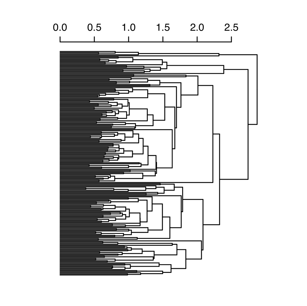
We will look closely at the changes between months (i) 21 and 22; (ii) 119, 120 and 121; and (iii) 172 and 173. From Figure 6, these correspond to the caesuras in moving through periods defined by (i) clusters of months 3, 4 and 5; (ii) clusters of months 5, 6 and 7; and (iii) clusters of months 7 and 8.

Since the 204 months are from January 1988 to December 2004, we determine these changes as being, respectively: (i) late (September, October) 1989; (ii) beginning of 1998 (December 1997, January and February 1998); and (iii) early 2002 (April, May 2002).

The 1989 changepoint, (i), as noted above (section 4.1 and [9]) was in the “adjustment period” due to the end of the Cold War and its influence on the Colombian civil strife.

The 1998 changepoint, (ii), was in a period when guerrilla gains from 1996 onwards were being reversed, a process that was seen to be so by 1999. There were high levels of government casualties in 1997–1998, due to guerrilla operations against isolated military and police bases. In particular through airborne weaponry, the government got the upper hand. The “upsurge period” from 1997 onwards also saw a rise of (anti-guerrilla) paramilitary activity whereas before they had been involved in drug trafficking. The paramilitaries started operations around 1997. There was a consolidation of paramilitary groups in 1997, announced publicly in December 1997, and they became active then, having many of their own number killed. It was not until 1999 that paramilitaries began to kill large numbers of guerrillas. Among all of these mutually influencing, reinforcing or retarding, trends and events, our analysis points to a succession of two months where the global change was most intense.

We now come to the 2002 changepoint, (iii). A peak of (paramilitary) casualties brought about by government against paramilitaries was in 2002 due to aerial bombardment of a paramilitary position under attack by guerrillas. It was a major setback for the paramilitaries, who declared a truce following the election that year of President Alvaro Uribe.

5 Conclusions

In our data mining examples we have shown how an ultrametric embedding is achieved, starting from the data. The $\chi^{2}$ metric is appropriate for frequencies of occurrence data. Points and associated masses in the dual spaces of observations and of attributes can be mapped from the $\chi^{2}$ distance to a Euclidean space. On the points in this, now of identical masses, a hierarchy associated with an ultrametric can be induced. We have described briefly in this work how such a hierarchy can be used to read off, and otherwise investigate, changepoints or anomalous occurrences at a range of scales.

Appendix: the Correspondence Analysis and Hierarchical Clustering Platform

This Appendix introduces important aspects of Correspondence Analysis and hierarchical clustering. Further reading is to be found in [2] and [7].

Analysis Chain

1. Starting point: a matrix that cross-tabulates the dependencies, e.g. frequencies of joint occurrence, of an observations crossed by attributes matrix.

2. By endowing the cross-tabulation matrix with the $\chi^{2}$ metric on both observation set (rows) and attribute set (columns), we can map observations and attributes into the same space, endowed with the Euclidean metric.

3. A hierarchical clustering is induced on the Euclidean space, the factor space.

Various aspects of Correspondence Analysis follow on from this, such as Multiple Correspondence Analysis, different ways that one can encode input data, and mutual description of clusters in terms of factors and vice versa. In the following we use elements of the Einstein tensor notation of [2]. This often reduces to common vector notation.

Correspondence Analysis: Mapping $\chi^{2}$ Distances into Euclidean Distances

• The given contingency table (or numbers of occurrence) data is denoted $k_{IJ}=\{k_{IJ}(i,j)=k(i,j);i\in I,j\in J\}$.

• $I$ is the set of observation indexes, and $J$ is the set of attribute indexes. We have $k(i)=\sum_{j\in J}k(i,j)$. Analogously $k(j)$ is defined, and $k=\sum_{i\in I,j\in J}k(i,j)$.

• Relative frequencies: $f_{IJ}=\{f_{ij}=k(i,j)/k;i\in I,j\in J\}\subset\mathbb{R}_{I\times J}$, similarly $f_{I}$ is defined as $\{f_{i}=k(i)/k;i\in I,j\in J\}\subset\mathbb{R}_{I}$, and $f_{J}$ analogously.

• The conditional distribution of $f_{J}$ knowing $i\in I$, also termed the $j$th profile with coordinates indexed by the elements of $I$, is:

  $$f^{i}_{J}=\{f^{i}_{j}=f_{ij}/f_{i}=(k_{ij}/k)/(k_{i}/k);f_{i}>0;j\in J\}$$

  and likewise for $f^{j}_{I}$.

Input: Cloud of Points Endowed with the Chi Squared Metric

• The cloud of points consists of the couples: (multidimensional) profile coordinate and (scalar) mass. We have $N_{J}(I)=$ $\{(f^{i}_{J},f_{i});i\in I\}\subset\mathbb{R}_{J}$, and again similarly for $N_{I}(J)$.

• Included in this expression is the fact that the cloud of observations, $N_{J}(I)$, is a subset of the real space of dimensionality $|J|$ where $|.|$ denotes cardinality of the attribute set, $J$.

• The overall inertia is as follows:

  $$M^{2}(N_{J}(I))=M^{2}(N_{I}(J))=\|f_{IJ}-f_{I}f_{J}\|^{2}_{f_{I}f_{J}}$$

  $$=\sum_{i\in I,j\in J}(f_{ij}-f_{i}f_{j})^{2}/f_{i}f_{j}$$

• The term $\|f_{IJ}-f_{I}f_{J}\|^{2}_{f_{I}f_{J}}$ is the $\chi^{2}$ metric between the probability distribution $f_{IJ}$ and the product of marginal distributions $f_{I}f_{J}$, with as center of the metric the product $f_{I}f_{J}$.

• Decomposing the moment of inertia of the cloud $N_{J}(I)$ – or of $N_{I}(J)$ since both analyses are inherently related – furnishes the principal axes of inertia, defined from a singular value decomposition.

Output: Cloud of Points Endowed with the Euclidean Metric in Factor Space

• The $\chi^{2}$ distance with center $f_{J}$ between observations $i$ and $i^{\prime}$ is written as follows in two different notations:

  $$d(i,i^{\prime})=\|f^{i}_{J}-f^{i^{\prime}}_{J}\|^{2}_{f_{J}}=\sum_{j}\frac{1}{f_{j}}\left(\frac{f_{ij}}{f_{i}}-\frac{f_{i^{\prime}j}}{f_{i^{\prime}}}\right)^{2}$$

• In the factor space this pairwise distance is identical. The coordinate system and the metric change.

• For factors indexed by $\alpha$ and for total dimensionality $N$ ($N=\mbox{ min }\{|I|-1,|J|-1\}$; the subtraction of 1 is since the $\chi^{2}$ distance is centered and hence there is a linear dependency which reduces the inherent dimensionality by 1) we have the projection of observation $i$ on the $\alpha$th factor, $F_{\alpha}$, given by $F_{\alpha}(i)$:

  $$d(i,i^{\prime})=\sum_{\alpha=1..N}\left(F_{\alpha}(i)-F_{\alpha}(i^{\prime})\right)^{2}$$ (1)

• In Correspondence Analysis the factors are ordered by decreasing moments of inertia.

• The factors are closely related, mathematically, in the decomposition of the overall cloud, $N_{J}(I)$ and $N_{I}(J)$, inertias.

• The eigenvalues associated with the factors, identically in the space of observations indexed by set $I$, and in the space of attributes indexed by set $J$, are given by the eigenvalues associated with the decomposition of the inertia.

• The decomposition of the inertia is a principal axis decomposition, which is arrived at through a singular value decomposition.

Hierarchical Clustering

Background on hierarchical clustering in general, and the particular algorithm used here, can be found in [5].

Consider the projection of observation $i$ onto the set of all factors indexed by $\alpha$, $\{F_{\alpha}(i)\}$ for all $\alpha$, which defines the observation $i$ in the new coordinate frame. This new factor space is endowed with the (unweighted) Euclidean distance, $d$. We seek a hierarchical clustering that takes into account the observation sequence, i.e. observation $i$ precedes observation $i^{\prime}$ for all $i,i^{\prime}\in I$. We use the linear order on the observation set.

Agglomerative hierarchical clustering algorithm:

1. Consider each observation in the sequence as constituting a singleton cluster. Determine the closest pair of adjacent observations, and define a cluster from them.

2. Determine and merge the closest pair of adjacent clusters, $c_{1}$ and $c_{2}$, where closeness is defined by $d(c_{1},c_{2})=\mbox{ max }\{d_{ii^{\prime}}$ $\mbox{ such that }i\in c_{1},i^{\prime}\in c_{2}\}$.

3. Repeat step 2 until only one cluster remains.

This is a sequence-constrained complete link agglomeration criterion. The cluster proximity at each agglomeration is strictly non-decreasing.

References

- [1] Benois-Pineau, J. and Khrennikov, A. Significance delta reasoning with p-adic neural networks: application to change detection in video. Computer Journal, in press, 2008. doi:10.1093/comjnl/bxm087
- [2] Benzécri, J.-P. L’Analyse des Données, Tome I Taxinomie, Tome II Correspondances, 2nd ed. Dunod, Paris, 1979.
- [3] Burnett, M. and Allison, J. Everybody Comes to Rick’s, screenplay, 1940.
- [4] McKee R. Story: Substance, Structure, Style, and the Principles of Screenwriting, Methuen, 1999.
- [5] Murtagh F. Multidimensional Clustering Algorithms, Physica-Verlag, Würzburg, 1985.
- [6] Murtagh F. On ultrametricity, data coding, and computation, Journal of Classification, 21, 167-184, 2004.
- [7] Murtagh F. Correspondence Analysis and Data Coding with R and Java, Chapman & Hall/CRC, 2005.
- [8] Murtagh F., Ganz A. and McKie S. The structure of narrative: the case of film scripts, Pattern Recognition, in press, 2008. http://arxiv.org/abs/0805.3799 (Discussed in: Z. Merali, Here’s looking at you, kid. Software promises to identify blockbuster scripts, Nature, 453, 708, 4 June 2008.)
- [9] Restrepo J., Spagat M. and Vargas J.F. The dynamics of the Colombian civil conflict: a new data set, Homo Oeconomicus, 21, 396–428, 2004.
- [10] Restrepo J. and Spagat M. Colombia’s tipping point?, Survival, 47, 131–152, 2004.
- [11] Restrepo J. and Spagat M. Civilian casualties in the Colombian conflict: a new approach to human security, 2004.
- [12] Restrepo J., Spagat M. and Vargas J.F. The severity of the Colombian conflict: cross-country datasets versus new micro data, Journal of Peace Research, 45, 99–115, 2006.
- [13] van Rijsbergen C.J. The Geometry of Information Retrieval, Cambridge University Press, 2004.