ETH Zurich, UNO D11, Universitätstr. 41, 8092 Zurich, Switzerland
Approximate Hamiltonian Statistics in Onedimensional Driven Dissipative Many-Particle Systems
Abstract
This contribution presents a derivation of the steady-state distribution of velocities and distances of driven particles on a onedimensional periodic ring. We will compare two different situations: (i) symmetrical interaction forces fulfilling Newton’s law of “actio = reactio” and (ii) asymmetric, forwardly directed interactions as, for example in vehicular traffic. Surprisingly, the steady-state velocity and distance distributions for asymmetric interactions and driving terms agree with the equilibrium distributions of classical many-particle systems with symmetrical interactions, if the system is large enough. This analytical result is confirmed by computer simulations and establishes the possibility of approximating the steady state statistics in driven many-particle systems by Hamiltonian systems. Our finding is also useful to understand the various departure time distributions of queueing systems as a possible effect of interactions among the elements in the respective queue [D. Helbing et al., Physica A 363, 62 (2006)].
pacs:
05.40.-aFluctuation phenomena, random processes, noise, and Brownian motion and 47.70.-nNonequilibrium gas dynamics and 89.40.-aTransportation1 Introduction
Classical many-particle systems such as ideal gases are characterized by the applicability of Newton’s laws of mechanics, which particularly includes the law of “actio = reactio”. With these basic laws, many fundamental properties can be derived, like the conservation of momentum and energy. Such many-particle systems are known as Hamiltonian systems. Even statistical physics and thermodynamics are based on these relationships.
But what would happen if the law of “actio = reactio” would not hold and the particle interactions would not fulfil momentum and energy conservation? One example of such a system are driven Brownian particles where many results for stationary distributions are available. However, in this system, interactions are taken into account only implicitely by a nonlinear friction function erdmannEPJB2000 , or by a symmetric interaction potential Haenggi-EPL1999 . In other systems such as vehicular traffic one would like to model the non-symmetric interactions between the particles (vehicles) explicitely. Would it still be possible to find (analytical) formulas for the stationary distributions of velocities and distances? In fact, although a statistical physics formalism for driven systems is needed, there are still not many results available. The existing results mainly concern the study of traffic-jam related condensation phenomena by means of the master equation Mahnke99 or the Fokker-Planck equation Kuehne02 .
These considerations have assumed certain arrival and departure rates to or from any forming vehicle clusters, but they have not explicitly represented the acceleration or deceleration dynamics of interacting vehicles in space and time, which may lead to dynamic self-organization phenomena such as emergent stop-and-go waves Helb-Opus . In the following, we will take this dynamics of interacting particles into account.
In fact, we are seeking for a method to treat dissipative driven many-particle systems in a similar way as Hamiltonian systems. The idea is that the dissipation in the system would be balanced by the effect of the driving force, at least in a closed (circular) system in the limit of large particle numbers. This idea has been used to evaluate the vehicle interaction potential FPE-preprint ; Krbalek_Helb ; helbing2006uia , but questioned to be applicable to systems with asymmetric, forwardly directed interactions. Moreover, the method has been restricted to a very limited number of potentials , as the normalization factor of the distance distribution could not be analytically determined in general.
For onedimensional classical Hamiltonian gases, many results have been previously derived in the framework of Random Matrix Theory RMT-book ; krbalek2001htf . According to this, if coupled to a thermal bath, the velocity distribution of gas particles is Gaussian and the distance distribution can be written as
| (1) |
where is the interaction potential, is the velocity variance (i.e. proportional to the temperature), and depends on the particle density. It would be very desireable to have a similar result for driven many-particle systems, as this would allow one to determine the interaction potential and interaction force among driven particles in the presence of fluctuations. Our hope is that, in the stationary state, the dissipative interactions and the driving term would somehow cancel out on average, so that the behavior would approximately correspond to a Hamiltonian system, as assumed in the Refs. Krbalek_Helb ; helbing2006uia ; krbalek2001htf ; krbalek2007edt ; Schuetz-PRE2000 .
In fact, in this paper we will show that this idea is correct for onedimensional systems in the limit of large particle numbers. Even forwardly directed dissipative driven many-particle systems behave approximately like Hamiltonian systems if they are far away from a dynamic instability.
Our paper is structured as follows: In the next section, we lay out the theoretical basis and derive the form of the onedimensional Hamiltonian as well as the conditions, under which it provides a correct description. In Sec. 3 we formulate the predictions in a form that can be tested by simulating representative many-particle systems. The actual simulations and their results are presented in Section 4, after which we conclude with a discussion.
2 Driven many-particle model with dissipative interactions
In the onedimensional driven-many particle system we discuss, point-like particles change their location in time according to the equation of motion
| (2) |
and their temporal velocity change is assumed to be given by the following stochastic acceleration equation:
| (3) |
Here, denotes the “free” or “desired” velocity and represents a white noise fluctuation term satisfying
| (4) |
where is a velocity-diffusion constant. The particle mass has been set to 1, and describes a repulsive interaction force, which depends on the particle distance . The term with allows to study different cases: corresponds to the classical case of symmetrical interactions in forward and backward direction, fulfilling the physical law of “actio = reactio”. corresponds to the case of forwardly directed interactions only, which is, for example, applicable to vehicles.
2.1 Fokker-Planck equation for velocities and distances
In order to determine the statistical distributions of the velocities and distances of particles , it is helpful to rewrite the above stochastic differential equation (Langevin equation) in terms of an equivalent Fokker-Planck equation. With the definitions
| (5) | |||||
| (6) |
this Fokker-Planck equation reads Ri89
| (7) | |||||
where we assume periodic boundary conditions and for a onedimensional ring of length with particles on it. In the following, we will show that the ansatz
| (8) |
is a stationary solution of the above Fokker-Planck equation, if the parameters and are properly chosen, and if the so-called interaction potential is defined by
| (9) |
In Eq. (8),
| (10) |
is the normalization constant, and the Lagrange parameter is required to meed the constraint determining the actual particle density. Moreover,
| (11) |
is the average velocity and
| (12) |
the velocity variance. In the following, we will restrict our investigation to the stationary case with and , which presupposes that the deterministic part of Eq. (3) fulfils the linear stability condition
| (13) |
(see Ref. EPJB2 for the method to determine this formula). Otherwise, dynamic patterns such as stop-and-go waves may emerge from the dissipative interactions of driven particles Helb-Opus . Notice that in the Hamiltonian case, , the stability condition is always satisfied. Furthermore, the factorization assumption (8) requires that all variables and are statistically independent from each other. According to numerical simulations, this is only the case if is much smaller than the right-hand side of (13), i.e., the system is far from the instability point.
With the ansatz (8), the three terms of the Fokker-Planck equation (7) can be written as
| (14) | |||||
| (15) | |||||
and
| (16) |
We will now use the fact that
| (17) |
for any -dependent variable , i.e. indices can be shifted because of the assumed periodic boundary conditions. In this way we find
| (18) | |||||
Remarkably, this equation does not depend on the Lagrange parameter anymore, which is needed to adjust to the particle density.
Note that ansatz (8) can only be a stationary solution with , if
| (19) |
This relationship corresponds to the fluctuation-dissipation theorem. Applying it also to the last term of Eq. (18) and using the decompositions and , we find
| (20) | |||||
and, with the factorization assumption (8) and shifting indices again according to (17), we obtain
| (21) |
We will distinguish the following cases:
- 1.
-
2.
In the case of forwardly directed interactions as in vehicle traffic () and vanishing correlations, we have
(22) The first factor vanishes because of , but the second factor disappears as well: Dividing Eq. (3) by and summing up over gives
(23) In the limit of large enough particle numbers , the left-hand side converges to , while the last term on the right-hand side converges to 0. In the assumed stationary case with and using , this implies
(24) because of .
We conclude that the factorisation ansatz (8) satisfies the Fokker-Planck equation (7) if either the momentum is conserved (), or if the single-particle gaps and velocities are independent from each other. Note that, in order to arrive at this conclusion, the special form (9) for the interaction potential, particularly the prefactor , is required.
2.2 Hamiltonian description
An alternative approach is the Hamiltonian description. For this purpose, let us investigate the Hamiltonian
| (25) |
If , we can derive the following relations:
| (26) | |||||
Comparing this with (20) shows that
| (27) |
Correspondingly, in the stationary state we have
| (28) | |||||
In order to investigate under which conditions the Hamiltonian is conserved in the statistical average, we will calculate for two different cases:
-
1.
In a conservative system with no fluctuations () and no dissipation (), we have , independently of whether the interactions are symmetric or forwardly directed.
-
2.
For many-particle systems with fluctuation terms and/or dissipation, one can show
(29) This can be found by multiplication of Eq. (3) with and calculation of the ensemble average, using the factorization ansatz (8). The first term on the right-hand side vanishes under the assumption of a stationary state. The second and the fourth term vanish because of . Therefore,
(30) and, together with Eq. (28), we arrive at
(31) That is, in the statistical average we have . The same is expected for the average Hamiltonian per particle, of systems with many particles. In fact, simulations show that fluctuates with amplitudes , while the Hamiltonian itself fluctates with amplitudes , which is consistent with equilibrium hydrodynamic systems. As a consequence, stationary driven dissipative systems behave approximately Hamiltonian, even if the interactions are forwardly directed and Newton’s law “actio = reactio” is violated. This is, why the Hamiltonian statistics
(32) (the canonical distribution) is an approximate stationary solution of our driven dissipative many-particle system. Note that the contribution in Eq. (8) gives just a constant prefactor and can be absorbed into the normalization factor.
In conclusion, the equilibrium solution (8) of conservative many-particle systems is also a good approximation for the steady-state solutions () of driven many-particle systems of kind (3) with asymmetrical interactions, driving and dissipation effects, if the system is large enough, i.e. (for small systems, we expect that fluctuations become essential), and if the correlations between the gaps and velocities are insignificant.
3 Application to stochastic traffic models
In this section, we will formulate the results of the previous section in a way that can be tested by means of simulating specific models.
3.1 Single-particle distributions
The factorisation (8) can be written in the form
| (33) |
i.e., the statistics of the particles can be described by the single-particle gap distribution function
| (34) |
and the single-particle velocity distribution
| (35) |
Here, is a normalization constant, a Lagrangian parameter ensuring the density constraint, the average velocity, and the velocity variance. With the exception of , all quantities are dependent on the particle density .
3.2 Gap distribution
The two constants and of the gap distribution (34) are determined using the normalisation condition
| (36) |
and the constraint that the average gap is equal to the inverse of the global density,
| (37) |
Defining the integrals
we get
| (38) |
For , we find the transcendental equation
| (39) |
Using Newton’s method with the initial guess with defined in Eq. (43), one obtains for the -th iteration
| (40) |
where the integrals on the right-hand side are evaluated at . It turns out that this method converges within very few iterations, unless . In this case, however, the second derivative of the effective potential (9) typically satisfies the condition
| (41) |
allowing an asympotic expansion of (34) that eventually leads to a Gaussian gap distribution,
| (42) |
with
| (43) |
Remarkably, the ranges of applicability of (40) and (42) generally overlap, allowing a fast and robust solution.
3.3 Velocity distribution and kinetic energy
Equation (35) states that, regardless of the density, of the potential, and of the directions of the interactions, the single-particle velocity distribution is Gaussian. The expectation value is equal to that of the stationary velocity without fluctating terms. Furthermore, the velocity variance satisfies the fluctuation-dissipation theorem (19), i.e., the average kinetic energy per particle should be given by
| (44) |
4 Results
In this section, we will show by means of computer simulations, that the main predictions (34), (35), and (44) are valid if the system is in a regime that is far from any collective instability. In order to quantify this condition, we observe from (13) that the system becomes linearly unstable if the relaxation time exceeds some critical value . Thus, controls the stability properties which allows us to define the dimensionless reduced control parameter
| (45) |
Note that denotes equilibrium, while the linear threshold is characterized by . In particular, in the momentum-conserving case , we have always . The condition “far away from the instability point” can be formulated by the condition .
4.1 Selected models
In order to obtain a specific model, the interaction force of the stochastic differential equation (3) has to be specified. We will simulate two types of interaction forces that are based on (i) the optimal-velocity model, and (ii) on a power law.
| Parameter | Value |
|---|---|
| Desired velocity | 30 m/s |
| Velocity relaxation time | 0.2 s |
| Interaction length | 20 m |
| Shape parameter | 0.5 |
| Symmetry parameter | 0 and 1 |
| Fluctuating force | |
| Density | 12 /km and 30 /km |
| Parameter | Value |
|---|---|
| Desired velocity | 30 m/s |
| Velocity relaxation time | 2 s |
| Interaction distance | 20 m |
| Acceleration | |
| Interaction exponent | 2 |
| Symmetry parameter | 0 and 1 |
| Fluctuating force | |
| Density | 10 /km |
4.1.1 Stochastic optimal-velocity model (sOVM)
In the stochastic optimal-velocity model (sOVM), the interaction force is given by helbing2006uia
| (46) |
where we assume the optimal-velocity function
| (47) |
Table 1 summarizes the meaning of the model parameters and the values used in the simulations. Notice that the conventional optimal-velocity model of Bando et. al. Bando-jphys is obtained for the special case and in the Eqs. (3) and (4), respectively.
The sOVM has the following properties: The expectation value of the velocity for stationary conditions is given by
| (48) |
Furthermore, the effective potential (9) can be calculated analytically, resulting in
| (49) |
where the prefactor is given by
| (50) |
The dynamics of this model becomes linearly unstable if the relaxation time exceeds the critical value given by
| (51) |
see Eq. (13). For the parameters specified in Table 1, , and /km, the critical value is given by . This corresponds to when the parameters of Table 1 are assumed.
4.1.2 Stochastic power law model (sPLM)
An alternative, more physics-oriented model assumes that the interaction forces obey a power law FPE-preprint ; Krbalek_Helb :
| (52) |
which, together with (2) and (3), results in the stochastic power-law model (sPLM). The associated effective potential (9) is given by
| (53) |
and the expectation value for the velocity is equal to
| (54) |
This model differs qualitatively from the stochastic OVM in the following aspects:
-
•
If , the stationary velocity becomes zero for a finite average gap, . In contrast, the stationary velocity of the sOVM for any is nonzero, even at maximum density, .
-
•
The potential (53) of the stochastic power-law model diverges for , while the potential (49) of the sOVM remains finite. For the chosen parameters and , we have = = . Consequently, any car approaching a standing vehicle with a velocity exceeding = 52 m/s will lead to a rear-end collision. This velocity decreases with increasing values of , reaching at the limit of linear stability. In contrast, no such collisions are possible in the stochastic power-law model. Nevertheless, this model can become linearly unstable as well.
4.2 Simulations
We have simulated a closed ring road of length for the sOVM, and for the sPLM. We also have simulated larger systems resulting in no significant differences. We have started the simulations with deterministic initial conditions , and , corresponding to a single-particle distribution function
| (55) |
where represents Dirac’s delta function. Since this initial condition does not correspond to a stationary solution, we have run the simulations for a transient time of 72 000 s, before recording the results for further 36 000 s.
For the numerical update, we have applied the explicit scheme
| (56) | |||||
| (57) |
where denotes the deterministic part of the right-hand side of Eq. (3), and are independent realisations of a Gaussian distributed quantity with zero mean and unit variance.
The velocity update (56) corresponds to decomposing the deterministic and stochastic parts of the accelerations. While the deterministic part corresponds to an Euler update, the stochastic part is a result of explicitely solving the stochastic differential equation
for the initial conditions at time . The solutions are realisations of random-walk trajectories, which are Gaussian distributed with expectation value zero, and variance .
Notice that, for sufficiently small update times, this update scheme should converge (in the statistical sense) to the true solutions of (2) and (3). In the simulations, we have set . To verify the convergence, we have also run some simulations with lower values of the time step (down to ) and found less than 1% deviation.
4.3 Gap distribution
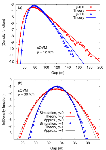
Figure 1 shows the simulated gap distributions for the stochastic OVM for two densities and two values of the symmetry parameter . For comparatively low densities (Fig. 1 (a)), both the predicted and the observed distributions are markedly asymmetric. Furthermore, the direction of interaction plays a role as well. For the limiting case of a car-following model (), the gap distribution is wider than in the symmetric (momentum-conserving) case . Generally, there is a good agreement between the theoretical expressions and the data. The only exception is the large-gap tail for symmetric forces at the lower density. In contrast, for the car-following case , even the tails are reproduced correctly (within statistical fluctuations). The same aggreement has been found for the higher density, irrespective of the value of . This is remarkable since additional assumptions have been necessary in Section 2 to derive the theoretical distributions for the car-following case. Consequently, one would expect larger errors compared to the isotropic case.
Now we investigate the influence of the densities on the form of the gap distribution. Comparing Fig. 1(a) with Fig. 1(b), one may conclude that, when increasing the density, the distributions become more and more symmetric. Further simulations showed that the distribution becomes significantly asymmetric if the single-particle kinetic energy exceeds the effective potential energy by at last one order of magnitude. Specifically, for the situation of Fig. 1, we have for all values of and while the effective potential energy corresponding to plot (a) is given by and that of plot (b) by .
For sufficiently high densities when the standard deviation of the gap distribution is much smaller than the average gap , the Gaussian assumption (42) should become valid. To determine the range of validity, we plotted the Gaussian approximation in the relevant Figure 1(b), in addition to the general distribution (34). For the case corresponding to , the Gaussian approximation agrees nearly perfectly with the full theoretical curve (the curves overlap with no visible difference). For (), however, a significant difference is found, but the distribution (34) already displays a significant skewness for this case. Further simulations showed that the Gaussian approximation is applicable whenever the full distribution (34) is sufficiently symmetric.
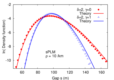
In order to evaluate the robustness of the predictions with respect to different model types, we have simulated the gap distributions for the stochastic power-law model as well. The results are shown in Fig. 2. Apart from minor deviations at the large-gap tails, we found a remarkable agreement between theory and simulation. Moreover, the predicted distributions for the car-following case and the symmetric case are significantly different both with respect to variance and shape, which justifies the particular specification (9) of the effective potential.
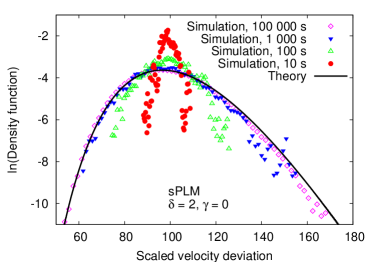
Finally, we looked closer at the relaxation dynamics of the initially -correlated distributions, Eq. (55), towards the stationary distributions. A very slow relaxation could be a possible reason for the deviations found sometimes at the large-distance tails of the gap distributions. In Fig. 3, we display snapshots of the evolution of the distribution for different simulation times. The results show that the relaxation time is considerable, particularly for low densities. Moreover, the relaxation process is particularly slow at the tails, so it may be a plausible reason for the remaining deviations.
4.4 Velocity distribution
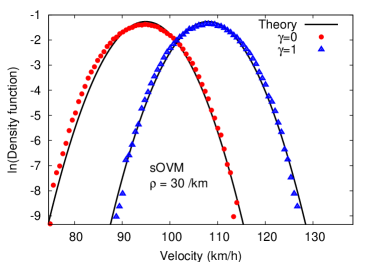
In contrast to the gap distributions, the predicted velocity distributions are always Gaussian. Moreover, the velocity variance should satisfy the fluctuation-dissipation theorem (19). As a consequence, the variance may neither depend on the density nor on the direction of the interacting forces. Figure 4 shows simulated velocity distributions for the stochastic OVM at the higher density corresponding to Fig. 1(b). One observes that, with the exception of small but systematic deviations from the Gaussian shape for the car-following case , all theoretical predictions are fulfilled. For the lower density (not shown), the agreement was nearly perfect for all values of .
In contrast to the gap distributions, the agreement of the velocity distributions improves when going from the car-following to the conservative case and when decreasing the density. This can possibly be explained by the distance from the instability point, see Eq. (13). For the densities and 30 /km, the dimensionless distances from the instability point are given by and , respectively, while we have for the conservative case. Obviously, the agreement increases with the degree to which the requirement is satisfied.
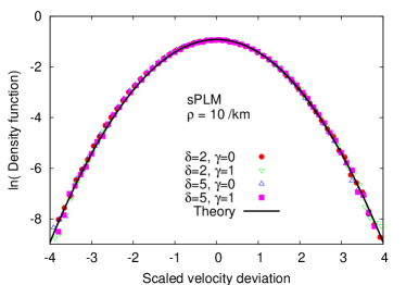
In Figure 5, we have plotted the simulated distributions for the stochastic power-law model for different values of the density and the directional parameter . In each simulation, we have normalized the distribution to the theoretical expectation value (54) and variance (19), so we expect that all curves collapse onto each other in the ideal case. This collapse is, in fact, observed, thanks to values of below for all cases.
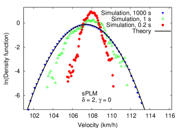
Finally, we investigate the relaxation process from the -correlated intial velocity distribution to the stationary distribution. Figure 6 shows that there is a significant scale separation for the relaxation times: While the typical velocity relaxation time scale is of the order of seconds, it is of the order of hundred seconds for the gap distribution. After 1 000 s, even the tails of the velocity distribution are perfectly equilibrated, while for the gaps, this takes longer by a factor of more than one hundred.
We conclude that, in contrast to the case of gap distributions, long relaxation times cannot explain possible differences between the theoretical and simulated velocity distributions, as noticeable in Fig. 4. These will be explained in the following.
4.5 Kinetic energy and correlations
One of the crucial assumption in the derivation of the gap and velocity distributions of Sec. 2 is the assumption of zero correlations, which requires that the system is far from any instability, i.e. . In classical thermodynamic systems, it is well known and theoretically understood landau-hyd that the energy contained in the fluctuations increases near a phase transition resulting in “critical opalescence” and other observable phenomena. The same has been found in driven thermodynamic systems such as Rayleigh-Bénard convection or electrohydrodynamic convection P-RMP-CrossHohenb-7v1-93 below the deterministic threshold, which will be further discussed in Sec. 5.
It is therfore very interesting to investigate the stochastic properties of our driven particle-systems as a function of the distance from threshold, i.e., varying the relaxation time from to or, equivalently, the control parameter from to .
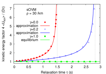
Figure 7 shows the single-particle kinetic energy of the fluctuations as a function of the relaxation time for several values of the directional parameter . The kinetic energy has been normalized to the value (44) resulting from the fluctuation-dissipation theorem (19). As in the physical systems mentioned above, we found significantly increased, so-called “critical fluctuations” near the linear threshold, which is located at for and at for while no such threshold exists for .
Finally, we compared the observed increase factor of the fluctation energy with the function of the scaled distance to the threshold (scaled control parameter). The agreement was astonishing for all investigated values of and .
5 Conclusion
In this contribution, we have investigated the statistical properties of onedimensional dissipative driven many-particle systems violating the law “actio = reactio”. Such systems can represent, for example, vehicular traffic or queuing systems with interactions.
In the theoretical derivation, we have shown that such systems approximately show a Hamiltonian statistic when inter-particle correlations play no significant role. The theoretical predictions were confirmed by simulations: Without a single free parameter to fit, we quantitatively obtained the typical characteristic properties of Hamiltonian systems such as velocity and gap statistics corresponding to a canonical ensemble when the Hamiltonian contains the usual contributions of kinetic and potential energy as in physical Hamiltonian systems. Furthermore, the velocity variance satisfied the fluctuation-dissipation theorem. As only prerequisite, we have found that the system must be far away from any instability point. This is consistent with the theoretical requirement of vanishing correlations, since collective instabilities such as stop-and-go traffic correspond to highly correlated particles.
In the first moment, these results appear to be quite surprising. For example, in traffic systems neither energy nor momentum are conserved during vehicle interactions, and the driving force keeps the system permanently far from equilibrium. While conservative systems conserve momentum and energy in each single interaction, in the driven dissipative systems studied by us, the additional relaxation term causes the average velocity to relax to the “free” or “desired” speed .
However, even systems violating the law “actio=reactio” may be mapped to effectively conservative systems by a Galilei transformation. Defining motions relative to the stationary velocity,
| (58) |
Eq. (3) becomes
| (59) |
One sees that the constant terms and resulting from the driving force and the relaxation dynamics supplement the interaction forces by counteracting forces – irrespective of the value of – such as in momentum-conserving systems.
One big difference of system not conserving momentum, however, remains when compared to conservative system: The conservative many-particle system always behaves dynamically stable, while the dissipative system potentially produces stop-and-go waves, when the linear stability condition 13 is not fulfilled. According to computer simulations, close to the instability point, the driven dissipative many-particle system tends to produce correlations between distances and velocities and between successive particles Schimansky-Geier-PRE98 .
This corresponds to pattern formation phenomena that would not occur in conservative systems. Such kinds of pattern formation phenomena have, for example, been investigated in fluid systems driven by thermal gradients (Rayleigh-Bénard convection), coriolis forces (Taylor-Couette flow), electrical fields (electroconvection), or concentration gradients (binary-mixture convection), see Ref. P-RMP-CrossHohenb-7v1-93 for a review. Moreover, the increase of thermal fluctations when approaching a linear stability threshold from below has been investigated theoretically and experimentally for the above systems Rehberg-EHC-fluct ; Ahlers-RBC-fluct ; Treiber-Taylor-fluct ; Rehberg-binMix2006 . Near the threshold but in the regime of linear response, the fluctuations should increase according to a power law, where the scaling exponents depend on the dimensionality and symmetry classes of the systems Treiber-EHC-fluct . Specifically, if the fluid systems are quasi-onedimensional, their fluctuations typically increase proportional to where the reduced control parameter is defined in analogy to Eq. (45), with replaced by a suitable driving force such as voltage or temperature gradient. Very near the threshold, however, deviations have been observed empirically Rehberg-PRL2000 .
It appears that in our case the fluctuations scale proportionally to as well. A theoretical foundation and a closer investigation of the above Fokker-Planck equation near the instability point and beyond will be subject of our future studies.
References
- (1) U. Erdmann, W. Ebeling, L. Schimansky-Geier, F. Schweitzer, The European Physical Journal B-Condensed Matter 15(1), 105 (2000)
- (2) P. Reimann, R. Kawai, C. Van den Broeck, P. Haenggi, EUROPHYSICS LETTERS 45(5), 545 (1999)
- (3) R. Mahnke, J. Kaupužs, Physical Review E 59(1), 117 (1999)
- (4) R. Kühne, R. Mahnke, I. Lubashevsky, J. Kaupužs, Physical Review E 65(6), 66125 (2002)
- (5) D. Helbing, Reviews of Modern Physics 73, 1067 (2001)
- (6) D. Helbing, M. Treiber, eprint arxiv:cond-mat/0307219 (2003)
- (7) M. Krbalek, D. Helbing, Physica A 333, 370 (2004)
- (8) D. Helbing, M. Treiber, A. Kesting, Physica A 363(1), 62 (2006)
- (9) M. Mehta, Random Matrices (Academic Press, 2004)
- (10) M. Krbalek, P. Šeba, P. Wagner, Phys. Rev. E 64(6), 066119 (2001)
- (11) M. Krbálek, Journal of Physics A: Mathematical and Theoretical 40(22), 5813 (2007)
- (12) T. Antal, G.M. Schütz, Phys. Rev. E 62(1), 83 (2000)
- (13) H. Risken, The Fokker-Planck Equation, 2nd edn. (Springer, Berlin, 1989)
- (14) D. Helbing, European Physical Journal B, submitted (2008)
- (15) M. Bando, K. Hasebe, K. Nakanishi, A. Nakayama, A. Shibata, Y. Sugiyama, Journal de Physique I France 5, 1389 (1995)
- (16) L. Landau, E. Lifshitz, Fluid Mechanics (Addison Wesley, Reading, MA, 1959)
- (17) M. Cross, P. Hohenberg, Rev.Mod.Phys. 65, 872 (1993)
- (18) A.A. Zaikin, L. Schimansky-Geier, Phys. Rev. E 58(4), 4355 (1998)
- (19) I. Rehberg, S. Rasenat, M. de la Torre Juárez, W. Schöpf, F. Hörner, G. Ahlers, H.R. Brand, Phys. Rev. Lett. 67(5), 596 (1991)
- (20) M. Wu, G. Ahlers, D. Cannell, Physical Review Letters 75(9), 1743 (1995)
- (21) M. Treiber, Physical Review E 53(1), 577 (1996)
- (22) W. Schöpf, I. Rehberg, Journal of Fluid Mechanics Digital Archive 271, 235 (2006)
- (23) M. Treiber, L. Kramer, Phys. Rev. E 49(4), 3184 (1994)
- (24) M.A. Scherer, G. Ahlers, F. Hörner, I. Rehberg, Phys. Rev. Lett. 85(18), 3754 (2000)