Toroidal field instability and eddy viscosity in Taylor-Couette flows

Abstract

Toroidal magnetic fields subject to the Tayler instability can transport angular momentum. We show that the Maxwell and Reynolds stress of the nonaxisymmetric field pattern depend linearly on the shear in the cylindrical gap geometry. Resulting angular momentum transport also scales linear with shear. It is directed outwards for astrophysical relevant flows and directed inwards for superrotating flows with ${\rm d}\Omega/{\rm d}R>0$. We define an eddy viscosity based on the linear relation between shear and angular momentum transport and show that its maximum for given Prandtl and Hartmann number depends linear on the magnetic Reynolds number $\mathrm{Rm}$. For $Rm\simeq 1000$ the eddy viscosity is of the size of $30$ in units of the microscopic value.

1 Introduction

Magnetic field configurations in astrophysical objects occur in wide variety. They play an essential role in the formation of flow pattern, are source and result of dynamo processes and enhance transport processes, where especially transport of angular momentum is of interest here. Crucial for magnetic field evolution is the interplay between toroidal and poloidal fields. In a differentially rotating environment for instance a weak poloidal field is wind-up into a strong toroidal one. A strong toroidal field on the other hand can become unstable due to the Tayler instability ([Tayler 1957, Tayler 1973, Vandakurov 1972]) or the Azimuthal magnetorotational instability (AMRI, see [Rüdiger et al. 2007]). As result also new components of a poloidal field are generated ([Gellert, Rüdiger & Fournier 2007]). To study in more detail the occurrence of the Tayler instability (TI) and especially the connected transport of angular momentum, we use a model in a cylindrical gap, that starts with an already dominating toroidal field and look for the fields instability in a differentially rotating environment.
Tayler instability mainly leads to nonaxisymmetric fields. This gives raise to the idea it could be part of a new dynamo mechanism caused only by the magnetic field ([Spruit 1999]). Even if there is a ongoing discussion if such a dynamo could really work ([Braithwaite 2006, Zahn, Brun & Mathis 2007, Gellert, Rüdiger & Elstner 2007, Rincon et al. 2008]), the TI might play an essential role for mixing of chemicals ([Rüdiger et al. 2008]), transport of angular momentum and resulting flattening of the rotation profile of stars. Estimates for angular momentum transport based on the so-called ’Tayler-Spruit’ dynamo are in use as input for star evolution models ([Maeder & Meynet 2005, Yoon, Langer & Norman 2006]). Putting such estimates on more robust basis is the aim of this work. It uses nonlinear 3D simulations of the Tayler instability in a cylindrical gap to compute the actual angular momentum transport

$$T=\langle u_{R}^{\prime}u_{\phi}^{\prime}-\frac{1}{\mu_{0}\,\rho}B_{R}^{\prime}B_{\phi}^{\prime}\rangle,$$ (1)

where field fluctuations are defined as nonaxisymmetric contributions of the whole velocity and magnetic field in cylindrical coordinates $(R,\phi,z)$. Further on it is shown that $T$ scales linear with the differential rotation, that is angular momentum transport can be expressed in terms of a positive turbulent or eddy viscosity $\nu_{\rm T}$. We find that for given shear and magnetic field strength always exists a maximum value of the eddy viscosity, which grows linearly with the magnetic Reynolds number $\mathrm{Rm}$.

2 Basic equations and numerics

We use the magnetohydrodynamic Fourier spectral element code described by Gellert, Rüdiger & Fournier (2007). With this approach we solve the 3D MHD equations

$$\partial_{t}\vec{u}+(\vec{u}\cdot\vec{\nabla}\!)\vec{u}=-\vec{\nabla}\!p+\vec{\nabla}\!^{\,2}\vec{u}+\frac{\mathrm{Ha}^{2}}{\mathrm{Pm}}(\mathrm{rot}\vec{B})\times\vec{B},$$ (2)

$$\partial_{t}\vec{B}=\frac{1}{\mathrm{Pm}}\vec{\nabla}\!^{\,2}\vec{B}+\mathrm{rot}(\vec{u}\times\vec{B}),$$ (3)

$$\mathrm{div}\vec{u}=0,\qquad\mathrm{div}\vec{B}=0$$ (4)

for an incompressible medium in a Taylor-Couette system with inner radius $R_{\mathrm{in}}$ and outer radius $R_{\mathrm{out}}$. Free parameters are the Hartmann number

$$\mathrm{Ha}=B^{0}_{\mathrm{in}}\sqrt{\frac{R_{\mathrm{in}}D}{\mu_{0}\rho\nu\eta}}$$ (5)

and the magnetic Prandtl number $\mathrm{Pm}=\nu/\eta$. Here $\nu$ is the viscosity of the fluid and $\eta$ its magnetic diffusivity. The Reynolds number is defined as $\mathrm{Re}=\Omega_{\mathrm{in}}R_{\mathrm{in}}D/\nu$ with $D=R_{\mathrm{out}}-R_{\mathrm{in}}$ (unit of length) and the angular velocity of the inner cylinder $\Omega_{\mathrm{in}}$. Unit of velocity is $\nu/D$ and unit of time the viscous time $D^{2}/\nu$.

The solution is expanded in $M$ Fourier modes in the azimuthal direction. This gives rise to a collection of meridional problems, each of which is solved using a Legendre spectral element method (see e.g. [Deville et al. 2002]). Either $M=8$ or $M=16$ Fourier modes are used, three elements in radial and eighteen elements in axial direction. The polynomial order is varied between $N=10$ and $N=16$. With a semi-implicit approach consisting of second-order backward differentiation formula and third order Adams-Bashforth for the nonlinear forcing terms time stepping is done with second-order accuracy ([Fournier et al. 2004]).

Boundaries at the inner and outer walls are assumed to be perfect conducting. In axial direction we use periodic boundary conditions to avoid perturbing effects from solid end caps. The periodicity in $z$ is set to $\Gamma=6D$.

The simulations start with an initial angular velocity profile

$$\Omega(R)=a+\frac{b}{R^{2}},$$ (6)

the typical Couette profile, with

$$a=\frac{\hat{\mu}_{\Omega}-\hat{\eta}^{2}}{1-\hat{\eta}^{2}}\Omega_{\mathrm{in}},\qquad b=\frac{1-\hat{\mu}_{\Omega}}{1-\hat{\eta}^{2}}R^{2}\Omega_{\mathrm{in}},$$ (7)

$\hat{\eta}=R_{\mathrm{out}}/R_{\mathrm{in}}=0.5$ and $\hat{\mu}_{\Omega}=\Omega_{\mathrm{out}}/\Omega_{\mathrm{in}}$. Following the Rayleigh stability criterion $\partial_{R}(R^{2}\Omega)^{2}>0$ a configuration with $\hat{\mu}_{\Omega}>0.25$ is hydrodynamically stable. This is always fulfilled in our computations. In addition to the shear flow a toroidal external field $\vec{B_{\mathrm{ext}}}=(0,B^{0},0)$ is applied. The second component $B^{0}$ has a radial profile similar to the flow with a component that is connected to a current only within the inner cylinder wall and a second with a current also within the fluid domain:

$$B^{0}(R)=a_{B}R+\frac{b_{B}}{R}.$$ (8)

Thus the external field than can be characterized by the number

$$\hat{\mu}_{B}=\frac{B^{0}_{\mathrm{out}}}{B^{0}_{\mathrm{in}}}=\frac{a_{B}R_{\mathrm{out}}+b_{B}R_{\mathrm{out}}^{-1}}{a_{B}R_{\mathrm{in}}+b_{B}R_{\mathrm{in}}^{-1}}.$$ (9)

The current-free field is given by $\hat{\mu}_{B}=0.5$. Values below lead to a field connected with constant negative current $j_{z}$ within the flow and larger values to a positive current. The TI occurs in the case that

$$\frac{\rm d}{{\rm d}R}(RB_{\phi}^{2})>0.$$ (10)

In the following $\hat{\mu}_{\mathrm{B}}$ is fixed to the value $\hat{\mu}_{\mathrm{B}}=1$. This means a nearly constant field along radial direction, which is unstable after the stability condition (10).

The initial magnetic field in the simulations consists of small random perturbations (white noise with an amplitude of $10^{-6}B^{0}_{\mathrm{in}}$).

3 Results

3.1 Tayler instability

The TI needs basically two conditions to be fulfilled to work. This is on one hand a strong enough magnetic field for given values of $\hat{\mu}_{\Omega}$ and $\hat{\mu}_{\mathrm{B}}$. And, on the other hand, it needs a not to high Reynolds number, because otherwise the instability is suppressed by the shear. In Rüdiger et al. (2007) stability maps for different Prandtl numbers resulting from a linear analysis are presented. The structure of all these maps for $\mathrm{Pm}\leq 1$ is roughly the same. For the case of $\mathrm{Pm}=0.1$ such a stability map is shown in Fig. 1 with values resulting from computations with the full 3D code. It differs only slightly from the linear results. Remarkable is the separation of the unstable region by a stable island. Nevertheless the appearance of the TI is in both regions the same. The most unstable mode is the nonaxisymmetric mode $m=1$. And in both regions exist a upper boundary for the Reynolds number where the instability disappears. With smaller $\mathrm{Pm}$ the critical Reynolds numbers grow. For $\mathrm{Pm}=1$ it is roughly $\mathrm{Re}=450$ for Hartmann number $\mathrm{Ha}=150$, for $\mathrm{Pm}=0.1$ already $\mathrm{Re}=1500$.

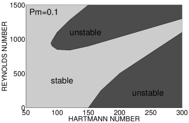
Figure 1: Stability map for TI with $\mathrm{Pm}=0.1,\hat{\mu}_{\Omega}=0.5$ and $\hat{\mu}_{\mathrm{B}}=1.0$. There exist two separated regions where the instability occurs.

3.2 Definition of eddy viscosity

For the calculation of the Maxwell and Reynolds stress we define mean fields as quantities averaged in azimuthal direction:

$$\langle\vec{u}\rangle=\frac{1}{2\pi}\oint\vec{u}\,{\rm d}\phi,\quad\langle\vec{B}\rangle=\frac{1}{2\pi}\oint\vec{B}\,{\rm d}\phi.$$ (11)

This regards nonaxisymmetric parts as fluctuations $\vec{u^{\prime}}=\vec{u}-\langle\vec{u}\rangle$ and $\vec{B^{\prime}}=\vec{B}-\langle\vec{B}\rangle$ respectively. The normalized equation for angular momentum transport (eq.1) then reads

$$T\simeq\langle u_{R}^{\prime}u_{\phi}^{\prime}\rangle-\frac{\mathrm{Ha}^{2}}{\mathrm{Pm}}\langle B_{R}^{\prime}B_{\phi}^{\prime}\rangle.$$ (12)

The question arising now is whether angular momentum is transported outwards, e.g. $T>0$ for ${\rm d}\Omega/{\rm d}R<0$. If this is true, an eddy viscosity $\nu_{\rm T}$ can be introduced by defining

$$T=-\nu_{\rm T}R\frac{{\rm d}\Omega}{{\rm d}R}$$ (13)

with positive $\nu_{\rm T}$.

Radial profiles of $T$ for $\mathrm{Pm}=1$, $\mathrm{Re}=30$, $\mathrm{Ha}=190$ and $\hat{\mu}_{\mathrm{B}}=1$ found in our nonlinear simulations are shown in Fig. 2. We find indeed that the value of $T$ depends on $\hat{\mu}_{\Omega}$. The profile is everywhere positive for $\hat{\mu}_{\Omega}<0.65$ and everywhere negative for $\hat{\mu}_{\Omega}>1.1$. For values in between there are regions where $T$ is positive or negative. Taking a radially averaged value of $T$ shows, that this average is positive for $\hat{\mu}_{\Omega}<0.75$ and negative for larger $\hat{\mu}_{\Omega}$.

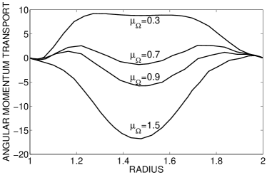
Figure 2: Radial profile of angular momentum transport $T$ for several differential rotation profiles $\hat{\mu}_{\Omega}$. Reynolds number is $\mathrm{Re}=30$ and Hartmann number $\mathrm{Ha}=190$. $T$ is mainly positive for subrotation $d\Omega/{\rm d}R<0$ and becomes negative for superrotation $d\Omega/{\rm d}R>0$.

It further on reveals a linear dependence between $T$ and $\hat{\mu}_{\Omega}$ in the whole range of $0.3<\hat{\mu}_{\Omega}<1.5$ (see Fig. 3). The kinetic part decreases with increasing $\hat{\mu}_{\Omega}$, it is zero for solid rotation as one would expect. Contrary the magnetic part increases with $\hat{\mu}_{\Omega}$ and is positive. The linear fit crosses zero at the Rayleigh line. There the pure hydrodynamic instability dominates and makes numerical checks impossible. The effect, that $T$ is not zero for solid rotation but has a contribution $T^{\ast}\sim\Omega$ is called $\Lambda$-effect ([Rüdiger 1989, Kichatinov & Rüdiger 1993]). Its appearance her is not yet investigated in detail.
Because of the linear scaling of $T$ with $\hat{\mu}_{\Omega}$, the introduction of an eddy viscosity as defined by eq. (13) is legitimate. If we substitute $R{\rm d}\Omega/{\rm d}R$ by using $\hat{\mu}_{\Omega}$ as

$$\frac{{\rm d}\Omega}{{\rm d}R}=(1-\hat{\mu}_{\Omega})\frac{R\Omega_{\mathrm{in}}}{D}$$ (14)

in eq. (13) and using the slope of the linear function $T=T(\hat{\mu}_{\Omega})$ plotted in Fig. 3, we get an eddy viscosity in units of the microscopic viscosity of $\nu_{\rm T}/\nu=0.39$ for the example with $\mathrm{Ha}=190$ and $\mathrm{Re}=30$. This is rather low and due to the fact that $\mathrm{Re}$ is chosen to be very small. In the astrophysically more relevant regime, where $\mathrm{Re}$ is (much) larger than $\mathrm{Ha}$ the eddy viscosity increases rapidly too.
Before describing the scaling of $\nu_{\rm T}$ with increasing Reynolds number and decreasing Prandtl number a remark regarding the size of the Maxwell and Reynolds stress is appropriate. As shown in Fig. 3 both values are of the same order. With increasing $\mathrm{Re}$ and $\mathrm{Ha}$ the magnetic part becomes more and more dominating. So the turbulent viscosity is mainly due to the magnetic field action. On the other hand, the velocity correlation stays on this low level. Arguing that the mixing of chemicals in stars is connected only to the kinetic part of the correlation tensor, mixing due to the TI would be rather weak ([Rüdiger et al. 2008]) and in agreement with observations of lithium concentration in solar type stars ([Brott et al. 2008]).

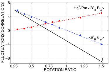
Figure 3: Scaling of angular momentum transport, Maxwell and Reynolds stress with the shear, expressed as rotation ratio $\hat{\mu}_{\Omega}$ of inner and outer cylinder. Positive $T$ means transport of angular momentum outwards.

3.3 Reynolds and Hartmann number dependence of eddy viscosity

To study the influence of turbulent viscosity for instance in star evolution models, one would like to have a relation at hand connecting the size of $\nu_{\rm T}/\nu$ with given (magnetic) Reynolds and Hartmann numbers. This are usually large values and are not reachable with our 3D simulations, thus a direct computation is impossible at the moment. Nevertheless, in a first step we want to give a scaling relation of $\nu_{\rm T}$ depending on $\mathrm{Re}$ and/or $\mathrm{Ha}$ for $0.1\leq\mathrm{Pm}\leq 1$.
As already mentioned the TI for given Hartmann number occurs only in a certain range for $\mathrm{Re}$. Along a line of constant $\mathrm{Ha}$ starting from the lower critical value of $\mathrm{Re}$ the instability first becomes stronger in a sense, that the angular momentum transport increases. It reaches a maximum and fades away towards the upper critical $\mathrm{Re}$. This behavior is shown in Fig. 4 for $\mathrm{Pm}=1$ and $\mathrm{Ha}=190$. The fit with a second order polynomial suggests a $T\sim{\rm Rm}^{2}$ scaling for the increasing part.

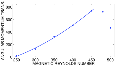
Figure 4: Angular momentum transport for $\mathrm{Pm}=1$, $\mathrm{Ha}=190$ with $\hat{\mu}_{\mathrm{B}}=1$ and $\hat{\mu}_{\Omega}=0.5$. The rotational stabilization for large $\mathrm{Re}$ leads to the existence of a maximum value. The fitted line, a parabola, suggests a relation $T\sim{\rm Rm}^{2}$.

The calculation of $\nu_{\rm T}$ from $T$ using eq. (13) gives the values plotted in Fig. 5. The dependence seems to be the same as for T: $\nu_{\rm T}\sim{\rm Rm}^{2}$ if far enough from the upper stability boundary. The maximum value in this example ($\mathrm{Ha}=190$) for the eddy viscosity is ${\rm max}(\nu_{\rm T}/\nu)=12.3$. It grows further when $\mathrm{Ha}$ is increased and reaches an absolute maximum of the order of 30 for $\mathrm{Ha}\approx 500$ for $\mathrm{Pm}=1$. For Prandtl numbers below $\mathrm{Pm}=1$, this tendency to reach a saturation value is not yet visible in the with our code achievable range for the Reynolds and Hartmann number respectively. The several computed values are listed in tab. 1. Because the Reynolds number grid is rather coarse, the given maxima might be slight underestimations of the real maxima, which reside between the given value and the first lower point towards the upper stability boundary.

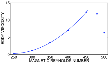
Figure 5: Same as in Fig. 4 but for the normalized eddy viscosity $\nu_{\rm T}/\nu$.

Table 1: Eddy viscosity $\nu_{\rm T}$ and the belonging Reynolds numbers for which $\nu_{\rm T}/\nu$ reaches its maximum for given Prandtl number and Hartmann number.

$\mathrm{Pm}$	$\mathrm{Ha}$	max$(\nu_{\rm T}/\nu)$	$\mathrm{Re}$
0.1	150	3.8	1300
0.4	100	5.7	550
0.4	150	9.2	850
0.4	250	17.6	1700
1.0	100	5.2	320
1.0	190	12.3	460
1.0	400	29.1	1100
1.0	500	30.4	1200

The next question we attack is if it is possible to find a relation between the eddy viscosity maxima and the parameters they depend on, and how such a relation will look like. The first idea is that such a relation should reflect the influence from all free parameters, thus a quantity depending on magnetic field, shear and Prandtl number. Thereby on aspect simplifies the problem: we deal only with the maxima. For them it is equivalent to use $\mathrm{Re}$ or $\mathrm{Ha}$, both are not independent. So the relation in question might hide the dependence on the third parameter. Two well-known parameters, the Lundquist number $S$ and the magnetic Reynolds number $\mathrm{Rm}$ combine the influence from two physical properties of the system. Both are first candidates to check. The plot of $\nu_{\rm T}(S)$ does not reveal a direct relation between eddy viscosity and Lundquist number and is not shown here.

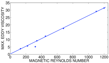
Figure 6: Linear dependence of eddy viscosity maxima on the magnetic Reynolds number for the investigated Prandtl number range $0.1\leq\mathrm{Pm}\leq 1$.

On the other hand a plot of $\nu_{\rm T}$ as function of $\mathrm{Rm}$ shows indications of the relation in question. Using the values of $\nu_{\rm T}/\nu$ listed in tab. 1 gives the data points plotted in Fig. 6. Those points reveal a linear dependence

$$\nu_{\rm T}/\nu=0.026\,\mathrm{Rm}+0.45$$ (15)

between eddy viscosity maxima and magnetic Reynolds number independent on Prandtl number. The one exceptional point much below the line for $\mathrm{Rm}=320$ is due to the fact, that this point, belonging to $\mathrm{Ha}=100$, is to close to the left stability boundary (see fig. 1, for $\mathrm{Pm}=1$ the Hartmann number range is very the same). Lets remind the reader that $\nu_{\rm T}$ here means the maxima of the eddy viscosity produced by the TI for given Prandtl and Hartmann (or equivalent Reynolds) number. As visible in Fig. 5 the linear relation $\nu_{\rm T}(\mathrm{Rm})$ is not true in general for arbitrary combinations of Hartmann and Reynolds numbers.

The derived relation (15) agrees also quite well with the resulting value for the eddy viscosity described in subsection 3.2 using the linear dependence between $T$ and the differential rotation parameter $\hat{\mu}_{\Omega}$. Indeed, going to higher Hartmann numbers leads to an increase of the eddy viscosity to a value of $\nu_{\rm T}/\nu=1.1$, which is nearly exactly the value relation (15) predicts for $\mathrm{Rm}=30$.

The scaling with $\mathrm{Rm}$ reflects the raising influence of the magnetic field fluctuations for faster rotation. It is derived for nearly constant magnetic fields ($\hat{\mu}_{\mathrm{B}}=1$) and a Prandtl number between $\mathrm{Pm}=0.1$ and $\mathrm{Pm}=1$. If we assume it holds also for smaller Prandtl numbers, one could expect for instance in young, fast rotating stars with $\mathrm{Rm}\approx 1000$ a significant transport of angular momentum and eddy viscosities of the order of $30$. For a sun-like star with $\mathrm{Rm}\approx 150$ it would be a weak effect with $\nu_{\rm T}/\nu=5$.

4 Conclusions

Strong toroidal fields under the influence of a differentially rotating medium can become unstable to nonaxisymmetric perturbations. This instability, the Tayler instability, appears only if the shear is not to strong. In cylindrical gap geometry for Prandtl numbers $0.1\leq\mathrm{Pm}\leq 1$ there is always an upper boundary for the Reynolds number above which the instability is suppressed. The smoothing action of differential rotation dominates. Additionally it needs the crossing of a threshold for the strength of the magnetic field, for a nearly constant toroidal field with $\hat{\mu}_{\mathrm{B}}=1$ this is of the order of $\mathrm{Ha}\approx 100$. If our astrophysical object in mind provides such requirements, the TI leads to nonaxisymmetric magnetic field pattern.

Using the nonaxisymmetric parts as fluctuations, the resulting angular momentum transport scales linear with the differential rotation, it is positive for astrophysical relevant configurations with $\hat{\mu}_{\Omega}\leq 0.75$, e.g. angular momentum is transported outwards. This gives raise to the introduction of an eddy viscosity which causes the additional turbulence in the underlying medium.

For a fixed magnetic field there is always an upper and lower critical Reynolds number in between the instability can be observed. And there is also a maximum value of angular momentum transport and eddy viscosity. Taking the maxima of the latter we find its values follow a linear dependence on the magnetic Reynolds number. A direct influence of the field strength is hidden behind the fact, that with the Reynolds number also the Hartmann number is fixed for the point where the eddy viscosity has its maxima.

The linear relation $\nu_{\rm T}(\mathrm{Rm})$ is derived for a simplified model with fixed toroidal field and without any influence from density stratifications for rather high Prandtl numbers $0.1\leq\mathrm{Pm}\leq 1$. Although, imagine it hold also for Prandtl numbers one or two orders of magnitude less, this relation could be used to estimate eddy viscosities usable as input for star evolution models. For instance for a young, fast rotating sun it gives values around $\nu_{\rm T}/\nu=30$.

References

- [Braithwaite 2006] Braithwaite, J.: 2006, A&A 449, 451
- [Brott et al. 2008] Brott I., Hunter I., Anders P., Langer N., 2008, astro-ph/0709.0874
- [Deville et al. 2002] Deville, M.O., Fischer, P.F., Mund, E.H.: 2002, High Order Methods for Incompressible Fluid Flow, Cambridge University Press
- [Fournier et al. 2004] Fournier, A., Bunge, H.-P., Hollerbach, R., Vilotte, J.-P.: 2004, GeoJI 156, 682
- [Gellert, Rüdiger & Elstner 2007] Gellert, M., Rüdiger, G., Elstner, G.: 2008, A&A 479, L33
- [Gellert, Rüdiger & Fournier 2007] Gellert, M., Rüdiger, G., Fournier, A.: 2007, AN 328, 1162
- [Kichatinov & Rüdiger 1993] Kichatinov, L. L., Rüdiger, G.: 1993, A&A 276, 96
- [Maeder & Meynet 2005] Maeder, A., Meynet, G.: 2005, A&A 440, 1041
- [Rincon et al. 2008] Rincon, F., Ogilvie, G.I., Proctor, M.R.E., Cossu, C. : AN 329, this issue
- [Rüdiger 1989] Rüdiger, G.: 1989, Differential rotation and stellar convection: Sun and solar-type stars, Akademie-Verlag Berlin
- [Rüdiger et al. 2008] Rüdiger, G., Gellert, M., Schultz, M.: 2008, MNRAS, submitted
- [Rüdiger et al. 2007] Rüdiger, G., Hollerbach, R., Schultz, M., Elstner, D.: 2007a, MNRAS 377, 1481
- [Spruit 1999] Spruit, H.C.: 1999, A&A 349, 189
- [Tayler 1957] Tayler, R. J.: 1957, Proc. Phys. Soc. B 70, 31
- [Tayler 1973] Tayler, R. J.: 1973, MNRAS 161, 365
- [Vandakurov 1972] Vandakurov, Yu. V.: 1972, SvA, 16, 265
- [Yoon, Langer & Norman 2006] Yoon, S.-C., Langer, N., Norman, C.: 2006, A&A 460, 199
- [Zahn, Brun & Mathis 2007] Zahn, J.P., Brun, A.S., Mathis, S.: 2007, A&A 474, 145