Survival benefits in mimicry: a quantitative framework

Abstract

Mimicry is a resemblance between species that benefits at least one of the species. It is a ubiquitous evolutionary phenomenon particularly common among prey species, in which case the advantage involves better protection from predation. We formulate a mathematical description of mimicry among prey species, to investigate benefits and disadvantages of mimicry. The basic setup involves differential equations for quantities representing predator behavior, namely, the probabilities for attacking prey at the next encounter. Using this framework, we present new quantitative results, and also provide a unified description of a significant fraction of the quantitative mimicry literature. The new results include ‘temporary’ mutualism between prey species, and an optimal density at which the survival benefit is greatest for the mimic. The formalism leads naturally to extensions in several directions, such as the evolution of mimicry, the interplay of mimicry with population dynamics, etc. We demonstrate this extensibility by presenting some explorations on spatiotemporal pattern dynamics.

I Introduction

Similarity between coexisting prey species is widely observed in nature. A less defended prey species, e.g., a less poisonous or more palatable species, may gain survival advantage by resembling a better defended prey species. Following the literature, we will refer to the lesser defended species as ‘mimic’ and the better defended one as ‘model’. Mimicry, being a prime example of evolution by natural selection, is a key topic in evolutionary theory and has been analyzed as such since Darwin’s time; some historical perspective is provided in Refs. JoronMallet_1998 ; MalletJoron_AnnRevEcolSyst99 ; Mallet_commentary_PNAS01 ; Sherratt_evolution-review2008 . Mimicry is also the subject of a growing number of experimental studies Speed-etal_wildbirds_ProcRSoc00 ; Ihalainen-etal_JornEvBiol07 ; Rowland-et-al_Nature07 ; BarberConner_acousticmimicry_PNAS07 ; Ihalainen-et-al_BehavEcoSociobiol08 . Despite its importance in evolutionary theory, mimicry has not received extensive treatment in the mathematical biology literature. In this article, we formulate a continuum framework describing the basic dynamics of mimicry and predation, which can serve as the foundation for a more quantitative direction of mimicry investigations.

The basic phenomenon of mimicry immediately raises a number of intriguing questions. Can the presence of a lesser-defended mimic species actually be advantageous to the unpalatable model? More broadly, what are the conditions for mimicry to be mutualistic rather than parasitic? Given fixed (un)palatabilities of each prey species and a certain population density of the model, what population density would provide optimal protection for the mimic species? These questions are already nontrivial in the simplified situation with two prey and one predator species, even in the absence of population dynamics, spatial variations, etc. In its full glory, mimicry dynamics presents a vast array of fascinating questions and phenomena. Only a small fraction of this promising field has been considered quantitatively.

Mathematical modeling of mimicry benefits appears already in Müller’s original nineteenth-century work (cf. Refs. JoronMallet_1998 ; Sherratt_evolution-review2008 ). More recently, some quantitative questions have been addressed mainly through computer simulation OwenOwen84 ; TurnerKearneyExton1984 ; huheey_AmNat88 ; speed93 ; TurnerSpeed_simulations96 ; TurnerSpeed_review99 ; Speed_RobotPredators_AnimBehav99 ; SpeedTurner_spectrum99 ; Darst_AnimBehav06 . Nevertheless, there is a relative shortage of mathematically well-defined questions and fully quantitative treatments, which we aim to address in this work.

We focus first on the simplest possible case, namely, two prey species and a predator species, with unlimited populations and constant densities $n_{1}$ and $n_{2}$ that are not depleted by predation. The predator attacks prey (model and mimic) at each encounter with probabilities $P_{1}$ and $P_{2}$. Predator learning is encoded via the modifications of $P_{1}$ and $P_{2}$ due to each attack event. The basic dynamics is illustrated schematically in Figure 1. Since the simplest version does not include population dynamics, the only dynamical variables are the attack probabilities $P_{1}$ and $P_{2}$. In computer simulations, each predator (in a predator ensemble) is associated with its own $P_{1}$, $P_{2}$ values. These values are modified via certain rules each time that predator attacks a prey. For our formulation, we also assume a large enough number of predators such that only average $P_{1}(t)$, $P_{2}(t)$ values are relevant. This allows us to write down differential equations for these dynamical variables. The resulting continuum description provides a context in which questions can be posed and answered with mathematical rigor. In addition to the questions we examine here for the simplified scenario, the framework also allows easy extension to more complex cases, such as varying population densities, spatial inhomogeneities and pattern formation, additional species, etc.

In several important cases, our differential equations allow exact analytic expressions for the time dependent functions $P_{1}(t)$, $P_{2}(t)$. These solutions reveal new effects, such as (1) transient answers to the mutualistic/parasitic question, which have strong implications for the interpretation of mimicry experiments; (2) an optimum density of palatable mimics at which mimicry most effectively provides survival benefits to the mimic. Our exact solutions also place on a firm mathematical footing and provide clearer understanding of some existing computer simulation results, such as the role of predator memory. In addition, we exploit the easy extensibility of our formulation to incorporate simple spatial dynamics and explore spatiotemporal density patterns — we report a “transmission” effect of spatial patterns between prey densities. Some further applications are presented in the appendix.

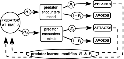
Figure 1: Predation and learning processes. The predator encounters prey at rates $n_{1}$ and $n_{2}$, and attacks them according to the probabilities $P_{1}$ and $P_{2}$ that characterize its behavior. Each attack event leads to learning, i.e., a modification of $P_{1}$ and $P_{2}$.

II The mathematical framework

The probability for a predator to encounter a model or mimic species is determined by their densities $n_{\mathrm{1}}$ and $n_{\mathrm{2}}$. We choose units such that $n_{\mathrm{1}}$, $n_{\mathrm{2}}$ are the encounter probabilities per unit time. Our dynamical variables are $P_{i}(t)$, the attack probabilities at each encounter. (The index $i$ runs over values 1 for the model and 2 for the mimic.)

The degree of defense for the model and mimic is characterized by “palatabilities” $\lambda_{1}$ and $\lambda_{2}$, which are the asymptotic attack probabilities for an infinite-memory predator trained by an infinite number of attack events. A larger $\lambda_{i}$ indicates a more palatable prey. As the mimic species emulates a more defended model species, we will use $\lambda_{1}\leq\lambda_{2}$. Since $\lambda_{i}$ are probabilities, they are restricted to lie between 0 and 1. We will use $P_{1}(0)=P_{2}(0)=P_{0}=0.5$ for the initial (naïve or “untrained”) attack probabilities.

Predator learning is modeled through the influence of attack events on $P_{1}$ and $P_{2}$ (figure 1). After a predator attacks a model, its $P_{1}$ value moves toward its asymptotic value $\lambda_{1}$, by an amount determined by the learning coefficient $\alpha$:

$$P_{1}\xrightarrow{\rm model\ attacked}P_{1}+\alpha[\lambda_{1}-P_{1}],$$ (1)

Since the predator cannot perfectly distinguish between model and mimic, the model attack probability also changes after a mimic attack event:

$$P_{1}\xrightarrow{\rm mimic\ attacked}P_{1}+r\alpha[\lambda_{2}-P_{1}].$$ (2)

Here $r$ is a resemblance coefficient representing the quality of mimicry; $r=0$ means no resemblance and $r=1$ means perfect resemblance. Since the average number of models attacked per unit time is $n_{1}P_{1}$ (figure 1), the model attack event of equation 1 contributes a term $n_{1}P_{1}\times\alpha(\lambda_{1}-P_{1})$ to the rate of change of $P_{1}$. With a similar contribution from equation 2, we obtain

$$\frac{dP_{1}}{dt}=\alpha n_{1}P_{1}[\lambda_{1}-P_{1}]+r\alpha n_{2}P_{2}[\lambda_{2}-P_{1}]+\gamma[P_{0}-P_{1}]\,.$$ (3)

In addition to the predator learning in equations (1,2), we have also included a “forgetting” term, quantified by a forgetting parameter $\gamma$. In the absence of learning events, the attack probability decays to the naïve value $P_{0}=0.5$. Similarly, for the mimic attack probability:

$$\frac{dP_{2}}{dt}=\alpha n_{2}P_{2}[\lambda_{2}-P_{2}]+r\alpha n_{1}P_{1}[\lambda_{1}-P_{2}]+\gamma[P_{0}-P_{2}]\,.$$ (4)

The analysis presented in this article is based on the coupled nonlinear equations (3,4) and variations or extensions thereof. Unless otherwise specified, we will generally be using $\alpha=1$, $n_{1}=n_{2}=0.5$.

The leading terms of (3,4) have the form of logistic equations well-known in population dynamics. However, our equations are for probabilities representing predator decision-making (not for populations or densities) and are based on quite different considerations.

In addition to the attack probabilities, another informative quantity in judging the benefits/losses of mimicry is the prey mortality, i.e. the number of prey that have been attacked by the time $t$:

$$N_{i}(t)=\int_{0}^{t}n_{i}P_{i}(t^{\prime})dt^{\prime}\;,\quad\quad[i=1,2]\;.$$ (5)

This quantity is particularly relevant in making contact with experimental data where mimicry advantages are usually reported in terms of prey mortalities Speed-etal_wildbirds_ProcRSoc00 ; Rowland-et-al_Nature07 . To quantify mimicry benefits, we will more often use the “favorability” ratio

$$f_{i}^{(r)}(t)~{}=~{}P_{i}^{(r=0)}(t)\;/\;P_{i}^{(r)}(t)\;,$$ (6)

especially its asymptotic value $f_{i}(t\rightarrow\infty)$. This ratio compares attack rates in non-resembling ($r=0$) and resembling ($r>0$) cases Mimicry is beneficial to model (mimic) if $f_{1}>1$ ($f_{2}>1$).

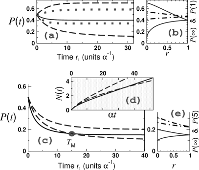
Figure 2: Results for infinite memory ($\gamma=0$).
(a,b) Attack probabilities for palatable mimic, $\lambda_{1}=0.1$, $\lambda_{2}=0.7$.
(a) Dashed, dotted: $r=0,0.4$. In each pair, lower (upper) curve represents model (mimic). Solid curve is $r=1$ probability, common for mimic and model.
(b) Dependence on resemblance. Dash-dot: $\alpha{t}=1$, solid: asymptotic. Model and mimic curves merge at $r=1$.
(c-e) Unpalatable mimic, $\lambda_{1}=0.1$, $\lambda_{2}=0.4$.
In (c,d), dashed pair are $r=0$ curves (upper: mimic, lower: model), and solid curves are common $r=1$ quantities.
(c) Attack probabilities. The solid $r=1$ curve crosses the lower dashed (model) $r=0$ curve at time $T_{\rm M}$ up to which mutualism persists. Mutualism corresponds to solid $r=1$ curve being lower than both dashed $r=0$ curves.
(d) Mortalities. Also displays the same transient phenomenon via a crossing of $r=1$ and model $r=0$ curves.
(e) Dependence on resemblance. Dash-dot: $\alpha t=5$, solid: asymptotic. The negative slope of the model (lower dash-dot) curve at finite time indicates the transient mutualism.

III Context: assumptions and relevance

III.1 Predator psychology

Obviously, the equations (3,4) make strong assumptions about the predation process. Learning and forgetting of avoidance are quantified through simple and reasonable rules. However, other rules could be argued to be equally reasonable (c.f., TurnerSpeed_review99 ; Speed_EvolEcology99 ; Sherratt_evolution-review2008 for detailed discussions). One alternative point of view TurnerKearneyExton1984 ; JoronMallet_1998 ; MalletJoron_AnnRevEcolSyst99 is that the asymptotic attack probability for defended prey should be always zero, and that the degree of defense (palatability) should be quantified only by differences in the learning rates $\alpha$. Müller’s original analysis also implicitly uses this picture of learning JoronMallet_1998 ; Sherratt_evolution-review2008 . Such a situation is conceivable when the predator has ample alternative sources of nourishment. Although our equations can be easily modified to incorporate such a picture of learning, we will here restrict ourselves to the case of nonzero asymptotic attack probabilities. This is supported by experiment Speed_EvolEcology99 , and presumably reflects the common situation where predator species are not fully saturated through alternate prey.

Predator behavior is an active topic of research and is not yet fully understood or characterized (c.f., Refs. Darst_AnimBehav06 ; Lynn_AnimBehav05 ; SkelhornRowe_AnimBehav06 ; Sherratt_evolution-review2008 ). Given the present level of understanding, it is reasonable to use the simplest way of quantifying predator training. Accordingly, we have mostly left out palatability-dependences of the learning rates, $\alpha(\lambda)=\alpha$, and also used the simplest description of forgetting. In the appendix, we include some variations of these simple assumptions when we seek to make generic statements, such as the (non)existence of mutualism with palatable prey. Refs. TurnerSpeed_simulations96 ; Speed_RobotPredators_AnimBehav99 ; SpeedTurner_spectrum99 describe various learning and forgetting rules used in the literature.

III.2 The palatability spectrum

One extreme of mimicry is the case where the mimic lacks defenses, i.e., is palatable, so that mimicry is parasitic with no benefit to the model. This is known as Batesian mimicry. At the other extreme, the two prey species could be equally defended, so that mimic and model are interchangeable labels. This is known as Muellerian mimicry. More interesting cases involve unequally defended prey, constituting a spectrum between the two extremes SpeedTurner_spectrum99 .

III.3 Benefits versus losses

Parasitism versus mutualism is a major theme of theoretical ecology (e.g., VandermeerGoldberg_book_PopulatnEcology03 ). In the mimicry context, the benefit/loss issue has been discussed with computer simulations, but unfortunately has not received as thorough a mathematical treatment as in other contexts. A formulation like the one we present in this Article is a necessary step in this direction.

III.4 Evolutionary implications

The issue of benefits versus losses in mimicry phenomena is important from an evolutionary perspective; there are vital implications for warning color diversity and polymorphism phenomena JoronMallet_1998 ; MalletJoron_AnnRevEcolSyst99 ; Mallet_commentary_PNAS01 ; Sherratt_evolution-review2008 ; Mallet_EvolEcology99 ; Servedio_Evolution00 . Our setting is well suited for addressing the basic question of whether mimicry is mutualistic or parasitic. A full quantitative study of evolutionary implications requires a more involved (perhaps multi-generation or many-species) framework. In the Supplementary Information we show how our formalism can be extended to address some of these themes.

III.5 Differential equation formulation

Our formulation is a continuum one, in contrast to the individual-predator simulations that have dominated theoretical mimicry studies. Such a setup opens up many new possibilities. It affords exact solubility for several important cases, even in the presence of forgetting. The formulation allows easy extension in several directions, such as spatial inhomogeneity, as we report below. It allows analytic tools, such as pattern formation theory, to be applied directly to such extensions. In addition, differential equations encourage us to study the complete predator training process, i.e., to focus on the dynamical aspects of mimicry. This is in contrast to existing literature which focuses on steady-state situations where the predator is already fully trained, which corresponds to the asymptotic behavior of our solutions.

Figure 3: Finite memory ($\gamma\neq 0$), $\lambda_{1}=0.1$.
(a,b) No asymptotic mutualism, $\lambda_{2}=0.4$, $\gamma=0.1$. (c,d) Asymptotic mutualism, $\lambda_{2}=0.15$, $\gamma=0.2$.
In (a) and (c) dashed lines show $r=0$ cases (lower - model, upper - mimic); solid lines show $r=1$ probabilities common to model and mimic. Note that (b,d) show asymptotic attack rates $P(\infty)$ only. The positive and negative signs of $dP_{1}/dr$ [slopes of lower curves in (b) and (d)] represent parasitism and mutualism respectively.
(e) Asymptotic model favorability. Solid, dashed, dash-dot: $\lambda_{2}=0.15,0.3,0.4$. Parameters corresponding to (a,b) and (c,d) are marked with circle and square respectively.
(f) Solid curve, $f_{1}(\gamma_{\rm min})=1$, separates mutualistic and and parasitic mimicry, dotted line indicates parameters optimum for model where $f_{1}(\gamma)$ has a maximum.

IV Example applications

IV.1 Infinite predator memory

We first report the dynamics of predator training with unlimited memory, $\gamma=0$. With no resemblance ($r=0$), equations (3,4) are not coupled and reduce to the logistic equation:

$$\frac{dP_{i}}{dt}~{}=~{}\alpha\,n_{i}P_{i}\;[\lambda_{i}-P_{i}],$$ (7)

which yields exact solutions for attack probabilities and mortalities:

$$P_{i}(t)=\frac{\lambda_{i}P_{0}}{P_{0}-(P_{0}-\lambda_{i})\exp(-\alpha n_{i}\lambda_{i}t)}\;,$$ (8)

$$N_{i}(t)=\frac{1}{\alpha}\ln[P_{0}(\exp(\alpha n_{i}\lambda_{i}t)-1)+\lambda_{i}]-\ln\lambda_{i}/\alpha\;.$$ (9)

The $P_{i}(t)$ here are logistic functions. The prey mortality grows linearly at small times ($N_{i}\sim{n_{i}P_{0}t}$) and also at asymptotically large times ($N_{i}\sim n_{i}\lambda_{i}{t}$), with mortality rates determined respectively by naïve and asymptotic attack probabilities ($P_{0}$ and $\lambda_{i}$).

For perfect resemblance, $r=1$, the solutions $P_{1}(t)$ and $P_{2}(t)$ are synchronized. Equations (3,4) collapse to one equation:

$$\frac{dP}{dt}=\alpha\,(n_{1}+n_{2})\,P\;[\bar{\lambda}-P]\;,$$ (10)

where $P=P_{1}=P_{2}$, and $\bar{\lambda}=(n_{1}\lambda_{1}+n_{2}\lambda_{2})/(n_{1}+n_{2})$. The $P(t)$ and mortalities for $r=1$ are given by the same equations (8,9) as in the $r=0$ case, with $n_{i}$ and $\lambda_{i}$ replaced by $(n_{1}+n_{2})$ and $\bar{\lambda}$ respectively.

Figure 2(a,c,d) displays typical time-dependences for attack probabilities and mortalities. The $P_{i}(t)$ start at their naïve value $P_{0}=0.5$ and tend to their asymptotic values, equal to $\lambda_{1}$ and $\lambda_{2}$ for non-resembling prey and to $\bar{\lambda}$ for the case of perfect resemblance.

For imperfect mimicry, $0<r<1$, the asymptotic solutions can still be found analytically, as the fixed points of the dynamical equations. It is also easy to obtain the complete time dependence numerically. Attack probabilities and mortalities vary monotonically between the perfect and zero resemblance cases described above (figure 2b and 2e). A negative slope of a $P_{i}$ versus $r$ curve indicates that mimicry is beneficial for that prey species.

IV.2 Asymptotes and transients

The infinite-memory equations predict that the presence of mimics is always harmful for models at sufficiently large times – the asymptotic model attack probability for $r>0$ is always larger than that for $r=0$, i.e., $P_{1}^{(r>0)}(\infty)>P_{1}^{(r=0)}(\infty)$. In other words, with this simplest version of predator psychology, mimicry is always parasitic in the long run, unless the prey species are equally defended ($\lambda_{1}=\lambda_{2}$).

However, our exact solutions display a surprising transient behavior, namely, for unpalatable but less-defended mimics ($\lambda_{1}<\lambda_{2}<P_{0}$), there is a finite time ($T_{\rm M}$) up to which mimicry can be favorable to the model, as displayed in figure 2c-e. In the transient regime $t<T_{\rm M}$, the slope $dP_{1}/dr$ for the model is negative. This transient mutualistic effect has not appeared previously in the literature, and has significant implications for the interpretation of mimicry experiments.

The appendix describes the extent of the transient regime in more detail.

IV.3 The predators forget

The inclusion of forgetting in the predator learning process has vital consequences for mutualism in mimicry. Some aspects, e.g., comparison of various memory mechanisms, have been treated through computer simulations speed93 ; TurnerSpeed_simulations96 ; SpeedTurner_spectrum99 ; Speed_RobotPredators_AnimBehav99 . Our formalism gives exact equations that quantify effects of finite predator memory, and reveals new effects. In particular, we explore the question of mutualism as a function of the rate of forgetting $\gamma$. We find a critical value of the forgetting parameter above which mimicry becomes asymptotically favorable to model.

We reinstate the memory parameter $\gamma$ in equations (3,4). With no resemblance ($r=0$), the decoupled equations have exact solutions

$$P_{i}=\frac{1}{2\alpha n_{i}}\Biggl{(}b_{i}+A_{i}\tanh\left[\frac{At}{2}-\mathrm{atanh}\Bigl{[}\frac{b_{i}-2\alpha n_{i}P_{0}}{A_{i}}\Bigr{]}\right]\Biggr{)}\;,$$ (11)

where $b_{i}=\alpha n_{i}\lambda_{i}-\gamma$ and $A_{i}=\sqrt{4\gamma P_{0}n_{i}\alpha+{b_{i}}^{2}}$. The asymptotic value is

$$P_{i}(t\rightarrow\infty)=\lambda_{i}/2+\frac{A_{i}-\gamma}{2\alpha n_{i}}\;.$$ (12)

Not surprisingly, $\gamma$ shifts the asymptotic attack probability from $\lambda_{i}$ toward the naïve value $P_{0}$. As in the $\gamma=0$ case, the perfect resemblance ($r=1$) solution ($P=P_{1}=P_{2}$) can be obtained from the $r=0$ solutions above, via $n_{i}\rightarrow(n_{1}+n_{2})$ and $\lambda_{i}\rightarrow\bar{\lambda}$.

The finite-memory learning process is illustrated by $P_{i}(t)$ curves in figures 3a,c. Figures 3a,b show a case with only transient mutualism. Figures 3c and 3d involve parameters (larger $\gamma$, smaller $\lambda_{2}$) where mimicry is mutualistic at all times. Figure 3e shows the asymptotic model favorability $f_{1}$ as a function of the forgetting rate $\gamma$. There is a threshold $\gamma=\gamma_{\rm min}$ above which the mimicry is mutualistic ($f_{1}>1$), and an optimum value at which $f_{1}>1$ is maximum (3e and 3f).

Figure 4: Non-monotonic dependence on mimic density.
(a) Mimic favorability $f_{2}$ versus relative mimic density $\delta=n_{2}/n_{1}$ (equation 13). Here $\lambda_{1}=0.1$, $\gamma=0.1$, $n_{1}+n_{2}=1$. Dotted, dashed, dash-dot, solid: $\lambda_{2}=0.3,0.6,0.8,1.0$. A maximum appears at large $\lambda_{2}$.
Insets show the optimum mimic density as a function of
(b) model palatability $\lambda_{2}$; (c) forgetting parameter $\gamma$.

IV.4 Optimum density

We now consider variable prey densities. We have found that the benefit of resemblance to the mimic can depend non-monotonically on the mimic density. In particular, for palatable mimics, $\lambda_{2}>P_{0}$, there is an optimum density, at which the asymptotic mimic favorability has a maximum. Again, our formulation provides an explicit expression describing this phenomenon:

$$f_{2}^{(r=1)}(\infty)=\frac{\lambda_{2}/2+(A_{2}-\gamma)/2\alpha n_{2}}{\bar{\lambda}/2+(\bar{A}-\gamma)/[2\alpha(n_{1}+n_{2})]}\;.$$ (13)

In figure 4a, we plot the favorability against the relative mimic density $\delta=n_{2}/n_{1}$, where $n_{1}+n_{2}=1$ is fixed. The non-monotonic behavior is robust; the optimum density $\delta_{\rm max}$ has very weak dependence on the resemblance $r$. The dependences of $\delta_{\rm max}$ on $\lambda_{2}$ and $\gamma$ are shown in figure 4b,c.

A prior example of non-monotonic density dependence OwenOwen84 ; Speed_RobotPredators_AnimBehav99 ; MalletJoron_AnnRevEcolSyst99 required unpalatable mimics ($\lambda_{2}<P_{0}$) and complicated forgetting rules. For example, the “variable forgetting” of Ref. Speed_RobotPredators_AnimBehav99 in our language would imply density-dependent $\gamma$. In contrast, we have found non-monotonic features and optima with a simple and transparent description of forgetting.

Understanding the density-dependence of mimicry benefits is crucial for studying mimicry together with population dynamics and evolution. A more detailed account of the density-dependence is provided in the appendix.

IV.5 Spatiotemporal dynamics and patterns

One attraction of our formulation is the ease of extension to studying spatiotemporal dynamics. We have tried the simplest cases of one-dimensional spatial dependence, with the densities $n_{i}(x,t)$ having growth and/or diffusion dynamics compensating the losses due to predation. This already supports a dramatic “pattern transmission” phenomenon, an example of which is shown in figure 5. Equations (3,4) for $P_{i}(x,t)$ (with $\gamma=0$) were supplemented by prey density equations:

$$\partial_{t}n_{1}(x,t)=-\beta_{1}n_{1}(x,t)P_{1}(x,t)+\tilde{\beta}_{1}~{}+~{}D_{1}\nabla^{2}n_{1}(x,t)\;,$$ (14)

$$\partial_{t}n_{2}(x,t)=-\beta_{2}n_{2}(x,t)P_{2}(x,t)+\tilde{\beta}_{2}~{}+~{}D_{2}\nabla^{2}n_{2}(x,t)\;.$$ (15)

A constant growth rate ($\tilde{\beta}_{i}$) is not extremely realistic but should be regarded as an effective description that provides a simple mechanism for constant nonzero asymptotic densities. The phenomenon we emphasize (transfer of inhomogeneity from one prey density to the other) is robust for a variety of growth and diffusion terms.

We find that a spatial variation (e.g., modulation) in the initial mimic density induces a spatial variation in model density, even when the two densities are not directly coupled. The predation ($P_{1}$, $P_{2}$ variables) mediate a coupling between the two prey species. The induced variation is “out of phase” for parasitic mimicry , i.e., a bump in mimic density causes a dip in model density, and “in-phase” for mutualistic cases. Figure 5 shows a parasitic example ($\lambda_{1}=0.1$, $\lambda_{2}=0.8$). The $\bar{\beta}_{i}$ and $D_{i}$ terms eventually smooth out all modulations. In figure 5, after the mimic modulation has died out the first time ($\alpha{t}\approx{5.3}$), the model density pattern in turn induces a modulation in the mimic density. Because mimicry is favorable to the mimic species, the re-induced modulation is now in-phase, opposite to the original mimic distribution. Figure 5 uses $D_{i}=0$; diffusion accelerates the smoothening process but the transmission effect is not qualitatively affected.

For the parameters we explored, there was no spontaneous pattern formation. However, our setup, when extended in spatial dimensions and additional dynamical processes, is clearly capable of a rich set of phenomena, waiting to be explored. In particular, equations (3,4) already contain “reaction” terms of the form $-P_{1}P_{2}$; it is therefore quite likely that spatial diffusion can induce patterns in some geometries, via, e.g, the Turing reaction-diffusion mechanism. Our framework provides the perfect setting for using the techniques of pattern formation theory CrossHohenberg_PatternFormation_RMP93 to analyze such phenomena.

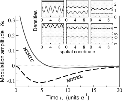
Figure 5: Pattern transmission: an initial spatial modulation of the mimic density is transfered to the model density, and then transmitted back to the mimic density with opposite the original phase.
The densities are of the form $n(x,t)=\bar{n}(t)+\delta{n}(t)\cos(kx)$. Main curves show modulation amplitudes $\delta{n}$. The sign of $\delta{n}$ indicates phase relative to the initial mimic modulation.
Six insets show model (upper) and mimic (lower) density profiles, at times (top row) $t=0,2,4$ and (lower row, note different scale) $t=6,10,15$.
(Parameters: $r=0.9$, $\beta_{1}=\beta_{2}=1.0$, $\bar{\beta_{1}}=0.3,\bar{\beta_{2}}=0.15$.)

V Conclusions

The topic of mimicry has received less mathematical attention than could be expected from its central importance to issues in evolutionary theory such as polymorphism and biodiversity. We have presented a framework which, although simple, has the advantage of being amenable to rigorous analysis and to extensions in various directions. In this regard, we recall the Lotka-Volterra equations in the mathematical study of predator-prey number dynamics, which are by themselves too simple to describe any ecological reality, but nevertheless provide the foundation for a vast area of theoretical ecology, due to their mathematical simplicity and rigor, and extensibility. We hope that our work will similarly stimulate quantitative developments in mimicry analysis.

Since the prime attraction of our formalism is its easy extensibility, we end by discussing three promising directions.

First, as illustrated through one example in figure 5, the inclusion of spatial dynamics opens fascinating pattern dynamics possibilities. Spatial distributions and mosaic structures in mimicry are active topics of ecological research Ellner-etal_spatial_JourMathBiol98 ; Sasaki-etal_mosaic_ThPopBiol02 ; JoronIwasac_spatial_JourTheorBiol05 ; Sherratt_spatial_JourTheorBiol06 ; KawaguchiSasaki_spatial_JourTheorBiol06 ; our formalism provides the groundwork for a unified mathematical treatment of some of the many intriguing phenomena.

Second, through the dynamics of our resemblance ($r$) parameter, our setup allows a basic description of evolutionary dynamics. (Some discussion is provided in the appendix). Incorporating more intricate descriptions of the evolution of resemblance remains an important open direction for future study.

Finally, with relatively small manipulations of our basic equations, experiments on mimicry can be modeled quantitatively. In this regard, the dramatic transient solutions we have provided may well turn out to be vital. For example, in a recent experiment Rowland-et-al_Nature07 , mutualistic behavior was found despite unequal prey defenses. Within our simple learning and forgetting rules, this can already have two different explanations: (a) the reported mutualism could be due to the transient effect described in figure 2c-e; (b) the observed mutualism could be a true asymptotic effect like the one found in the finite-memory cases, figure 3c-f. Since Ref. Rowland-et-al_Nature07 records data after a fixed mortality, it is not immediately obvious which period of the training dynamics the data corresponds to. However, the basic analysis of this article already provides a framework within which such questions can be addressed. The interpretation of experimental data is thus one more promising application of our work.

Appendix

In the appendix we describe

1. the time up to which transient mutualism exists;

2. dependence on mimic density;

3. further applications of our formalism.

.1 Transient mutualism

With infinite-memory predators, we have shown that although mimicry is not mutualistic (favorable to both prey species) in the long run, there is a part of the training period where temporary mutualism holds. In figure 6, we explore this phenomenon further by plotting the time ($T_{\rm M}$) up to which transient mutualism persists, against various parameters. The parameter $T_{\rm M}$ is defined pictorially in figure 2 of the main text.

The plot against the resemblance parameter $r$ shows (figure 6a) that the phenomenon is very robust. The transient time $T_{\rm M}$ changes little when the resemblance is varied from perfect to almost non-existent.

In figure 6b, the mimic palatability is varied. The phenomenon only occurs for $P_{0}>\lambda_{2}>\lambda_{1}$. The curve diverges for $\lambda_{2}\rightarrow\lambda_{1}$, which indicates that asymptotic mutualism is possible for equally defended prey ($\lambda_{2}=\lambda_{1}$).

It is also instructive to plot $T_{\rm M}$ against the memory parameter $\gamma$ (figure 6c). The transient time $T_{\rm M}$ increases with forgetting rate $\gamma$ and diverges at a critical value, denoted by $\gamma_{\rm min}$ in figure 3 of the main article. The divergence indicates that asymptotic mutualism appears above $\gamma=\gamma_{\rm min}$.

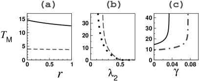
Figure 6: Time, $T_{\rm M}$, up to which transient mutualism persists.
(a) Plotted against resemblance paratmer $r$, with $\gamma=0$ and $\lambda_{1}=0.1$. Solid: $\lambda_{2}=0.2$; dashed: $\lambda_{2}=0.35$.
(b) Plotted against mimic palatibility $\lambda_{2}$, with $r=1$ and $\gamma=0$. Dotted: $\lambda_{1}=0.1$; dashed: $\lambda_{1}=0.2$. The divergences show that for infinite predator memory asymptotic mutualism only occurs for $\lambda_{2}=\lambda_{1}$.
(c) Plotted against memory parameter $\gamma$, with $r=1$ and $\lambda_{1}=0.1$. Solid: $\lambda_{2}=0.2$; dash-dotted: $\lambda_{2}=0.25$. The divergences show that mutualism becomes asymptotic above a critical value of the forgetting rate $\gamma$.

.2 Density-dependence

We describe the effect of mimic density on the survival benefits. We vary the relative mimic density $\delta=n_{2}/n_{1}$, with fixed $n_{1}+n_{2}=1$.

With an infinite-memory predator ($\gamma=0$), the asymptotic attack probabilities are simply the palatabilities $\lambda_{1}$ and $\lambda_{2}$ for non-resembling prey ($r=0$), independent of the densities. The $r=1$ asymptote $\bar{\lambda}=(n_{1}\lambda_{1}+n_{2}\lambda_{2})/(n_{1}+n_{2})$ depends on densities. The asymptotic mimic favorability

$$f_{2}=\frac{\lambda_{2}}{\bar{\lambda}}=\frac{\lambda_{2}(1+\delta)}{(\lambda_{1}+\lambda_{2}\delta)}\;$$

monotonously decreases with $\delta$ from $f_{2}(\delta\to 0)=\lambda_{2}/\lambda_{1}$ to $f_{2}(\delta\to\infty)=1$. The density dependence comes entirely from the denominator.

A finite predator memory ($\gamma\neq 0$) makes the situation more complicated. Now the $r=0$ asymptotes also depend on density, because the asymptotic attack probabilities are determined by the competition between learning and forgetting. The learning pulls the attack probabilities $P_{i}$ towards the palatibilities $\lambda_{i}$, while the forgetting tries to push them back to the naive value $P_{0}$. With increasing relative density $\delta$, the learning process becomes more important compared to the forgetting process, which is density-independent, so that the asymptotic $P_{i}$ get closer to the palatibilities $\lambda_{i}$. For palatable mimics ($\lambda_{2}>0.5$), the $P_{2}^{(r=0)}(t\rightarrow\infty)$ monotonically increases with relative mimic density $\delta$. The finite-$r$ asymptote, $P_{2}^{(r>0)}$, also grows with $\delta$, but at a different rate, and as a result the ratio (favorability) can depend non-monotonically on $\delta$, as illustrated in the main text.

.3 Further applications and extensions

We outline below some further applications of our formulation.

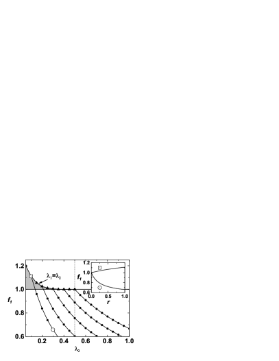
Figure 7: Search for mutualism with palatable mimic.
Asymptotic model favorability $f_{1}^{(r=1)}$ as a function of mimic palatability $\lambda_{2}$, obtained with cubic forgetting term $\gamma_{\rm c}(P_{0}-P_{1,2})^{3}$, where $\gamma_{\rm c}=5\times 10^{-4}$. The sequence of $f_{1}$-vs-$\lambda_{2}$ curves (filled circles) each correspond to a different value of $\lambda_{1}$, ranging from 0.1 for the leftmost curve to 0.5 for the rightmost. The tops of these curves (filled triangles) correspond to equally defended prey, $\lambda_{1}=\lambda_{2}$. Shaded area indicates the region of mutualistic mimicry ($f_{1}>1$) — clearly confined to $\lambda_{2}<0.5$, thus yielding a negative answer to the “mutualism with palatable mimic” question.
Inset shows, for one mutualistic ($f_{1}>1$) and one parasitic ($f_{1}<1$) case, that the dependence on resemblance coefficient $r$ is monotonic, so that the same negative answer holds for arbitrary $r$.

.3.1 Mutualistic mimicry with palatable mimic?

The ease of calculations with the differential-equation setup encourages us to ask more challenging questions, e.g., is there a situation in which a palatable mimic can be favorable for a defended model? Within our formulation, this means asking whether one can have benefit to the model ($f_{1}>1$) when $\lambda_{1}<P_{0}<\lambda_{2}$.

For both perfect ($r=1$) and imperfect ($0<r<1$) mimicry, our exact asymptotic solutions [of equations (3,4) in the main text] give a negative answer for the above question: mutualistic mimicry requires $\lambda_{2}<P_{0}$.

To explore the question further, we have studied several modifications of our basic equations, in particular
(A) using a palatability-dependent learning coefficient, $\alpha(\lambda)=\alpha_{0}(0.5+|\lambda-0.5|)$, as in Ref. speed93 ;
(B) replacing the linear forgetting term in equations (3,4) by various nonlinear forms, such as $\gamma_{\rm c}(P_{0}-P)^{3}$ or $\tilde{\gamma}(P_{0}^{2}-P^{2})$.
None of these variants of predator behavior allowed for mutualistic mimicry when $\lambda_{1}<P_{0}<\lambda_{2}$. Although the negative statement is impossible to prove strictly, our results indicate that mutualistic mimicry generically does not occur for palatable mimic species, at least within a wide class of approximations formulated within the framework represented in figure 1 in the main article. In figure 7, we demonstrate the absence of mutualism for one of the variants we have treated.

.3.2 Resemblance and discrimination

Our last example application is motivated by the fact that mimicry is rarely perfect in nature. The evolution of imperfect resemblance and the result of predator discrimination errors are important active topics in evolutionary theory MacDougallDawkins_AnimBehav98 ; GavriletsHastings_coevolutionary_JTheorBiol1998 ; Edmunds_imperfect-mimiry_Linnean00 ; Johnstone_imperfect-mimiry_Nature02 ; Sherratt_imperfect-mimiry_BehavEcol2002 . In our formalism, the ability of the predator to discriminate between prey species (or the degree of resemblance) is parametrized by a continuous variable $r$, providing the opportunity to explore the whole resemblance spectrum. For example, figures 2b, 2e, 3b, 3d plot attack probabilities as a function of the resemblance spectrum.

The evolution of resemblance can be thought of as modification of the $r$ variable. We can interpret the $r$-dependence of the attack probabilities: $dP/dr$ measures the driving force for evolutionary change. We can treat evolutionary dynamics by allowing $r$ to be a dynamical variable itself. The simplest equation would be of the type

$$\frac{dr}{dt}~{}=~{}-\epsilon_{1}\frac{\partial P_{1}}{\partial r}~{}-\epsilon_{2}\frac{\partial P_{2}}{\partial r}$$

Our formalism is thus potentially well-suited for a simple mathematical description of the dynamics of resemblance evolution.

- (1) M. Joron and J. L. B. Mallet, Diversity in mimicry: paradox or paradigm?, Trends in Ecology & Evolution, 13 (1998), pp. 461-466.
- (2) J. L. Mallet and M. Joron, Evolution of diversity in warning colour and mimicry: Polymorphisms, shifting balance, and speciation, Annu. Rev. Ecol. Syst. 30 (1999), pp. 201-233.
- (3) J. Mallet, Mimicry: An Interface between Psychology and Evolution, PNAS, 98, (2001), pp. 8928-8930.
- (4) T. N. Sherratt, The evolution of Müllerian mimicry, Naturwissenschaften 95 (2008), pp. 681-695.
- (5) M. P. Speed, N. J. Alderson, C. Hardman, and G. D. Ruxton, Testing Müllerian mimicry: an experiment with wild birds, Proc. Royal Soc. Lond. B 267 (2000), pp. 725-731.
- (6) E. Ihalainen, L. Lindström, and J. Mappes, Investigating Müllerian mimicry: predator learning and variation in prey defences, Journal of Evolutionary Biology, 20 (2007), pp. 780-791.
- (7) H. M. Rowland, E. Ihalainen, L. Lindström, J. Mappes, and M. P. Speed, Co-mimics have a mutualistic relationship despite unequal defences, Nature 448 (2007), pp. 64-66.
- (8) J. R. Barber and W. E. Conner, Acoustic mimicry in a predator-prey interaction, PNAS 104 (2007), pp. 9331-9334.
- (9) E. Ihalainen, I. L. Lindström, J. Mappes and S. Puolakkainen, Butterfly effects in mimicry? Combining signal and taste can twist the relationship of Müllerian co-mimics, Behavioral Ecology and Sociobiology, 62, (2008), pp. 1267-1276.
- (10) R. E. Owen and A. R. G. Owen, Mathematical paradigms for mimicry – recurrent sampling, J. Theor. Biol. 109 (1984), pp. 217-247.
- (11) J.R.G. Turner, E.P. Kearney and L.S. Exton, Mimicry and the Monte Carlo predator: the palatability spectrum and the origins of mimicry, Biological Journal of the Linnean Society, 23 (1984), pp. 247-268.
- (12) J. E. Huheey, Mathematical models of mimicry, American Naturalist 31 (1988), pp. s22-s41.
- (13) M. P. Speed, Muellerian mimicry and the psychology of predation, Animal Behaviour, 45 (1993), pp. 571-580.
- (14) J. R. G. Turner and M. P. Speed, Learning and memory in mimicry. I. Simulations of laboratory experiments, Philosophical Transactions: Biological Sciences, 351, (1996), pp. 1157-1170.
- (15) J. R. G. Turner and M. P. Speed, How weird can mimicry get?, Evolutionary Ecology, 13 (1999), pp. 807-827.
- (16) M. P. Speed, Robot predators in virtual ecologies: the importance of memory in mimicry studies, Animal Behaviour 57 (1999), pp. 203-213.
- (17) M. P. Speed and J. R. G. Turner, Learning and memory in mimicry: II. Do we understand the mimicry spectrum?, Linnean Society. Biological Journal 67 (1999), pp. 281-312.
- (18) C. R. Darst, Predator learning, experimental psychology and novel predictions for mimicry dynamics, Animal Behaviour 71 (2006), pp. 743-748.
- (19) M. P. Speed, Batesian, quasi-Batesian or Müllerian mimicry? Theory and data in mimicry research, Evol. Ecol. 13, (1999), pp. 755-776.
- (20) S. K. Lynn, Learning to avoid aposematic prey, Animal Behaviour, 70 (2005), pp. 1221-1226
- (21) J. Skelhorn, C. Rowe, Prey palatability influences predator learning and memory, Animal Behaviour, 71 (2006), pp. 1111-1118.
- (22) J. H. Vandermeer and D. E. Goldberg, Population Ecology: First Principles, Princeton University Press (2003).
- (23) J. Mallet, Causes and consequences of a lack of coevolution in Müllerian mimicry, Evol. Ecol. 13, (1999), pp. 777-806.
- (24) M.R. Servedio, The effects of predator learning, forgetting, and recognition errors on the evolution of warning coloration, Evolution, 54 (2000), pp. 751-763.
- (25) M. C. Cross and P. C. Hohenberg, Pattern formation outside of equilibrium, Reviews of Modern Physics, 65 (1993), pp. 851-1112.
- (26) A. MacDougall and M. S. Dawkins, Predator discrimination error and the benefits of Müllerian mimicry, Animal Behaviour, 55 (1998), pp. 1281-1288.
- (27) S. Ellner, A. Sasaki, Y. Haraguchi and H. Matsuda, Speed of invasion in lattice population models: pair-edge approximation, Journal of Mathematical Biology 36 (1998), pp. 469-484.
- (28) A. Sasaki, I. Kawaguchi and A. Yoshimori, Spatial Mosaic and Interfacial Dynamics in a Müllerian Mimicry System, Theoretical Population Biology, 61, (2002), pp. 49-71.
- (29) M. Joron and Y. Iwasac, The evolution of a Müllerian mimic in a spatially distributed community, Journal of Theoretical Biology, 237, (2005), pp. 87-103.
- (30) T. N. Sherratt, Spatial mosaic formation through frequency-dependent selection in Müllerian mimicry complexes, Journal of Theoretical Biology, 240, (2006), pp. 165-174.
- (31) I. Kawaguchi and A. Sasaki, The wave speed of intergradation zone in two-species lattice Müllerian mimicry model, Journal of Theoretical Biology, 243, (2006), pp. 594-603.
- (32) S. Gavrilets and A. Hastings, Coevolutionary Chase in Two-species Systems with Applications to Mimicry, Journal of Theoretical Biology, 191 (1998), pp. 415-427.
- (33) M. Edmunds, Why are there good and poor mimics? Biological Journal of the Linnean Society, 70 (2000), pp. 459-466.
- (34) R. Johnstone, The evolution of inaccurate mimics, Nature, 418, (2002), pp. 524-526.
- (35) T. N. Sherratt, The evolution of imperfect mimicry, Behavioral Ecology, 13 (2002), pp. 821-826.