Cosmological tachyon condensation

Abstract

We consider the prospects for dark matter/energy unification in k-essence type cosmologies. General mappings are established between the k-essence scalar field, the hydrodynamic and braneworld descriptions. We develop an extension of the general relativistic dust model that incorporates the effects of both pressure and the associated acoustic horizon. Applying this to a tachyon model, we show that this inhomogeneous “variable Chaplygin gas” does evolve into a mixed system containing cold dark matter like gravitational condensate in significant quantities. Our methods can be applied to any dark energy model, as well as to mixtures of dark energy and traditional dark matter.

1 Introduction

The discovery of the accelerated Hubble expansion in the SNIa data [1], combined with observations of the cosmic microwave background (CMB) [2, 3], has forced a profound shift in our cosmological paradigm. If one makes the conservative assumptions of the validity of Einstein’s general relativity and the cosmological principle, one concludes that the universe is presently dominated by a component that violates the strong energy condition, dubbed dark energy (DE). Moreover, primordial nucleosynthesis constrains the fraction of closure density in baryons, $\Omega_{B}$, to a few percent, while galactic rotation curves and cluster dynamics imply the existence of a nonbaryonic dark matter (DM) component with $\Omega_{DM}\gg\Omega_{B}$ (for a review see [4]). Currently, the best fit values are $\Omega_{B}=0.04,\Omega_{DM}=0.22$ and $\Omega_{DE}$ = 0.74 [3]. Thus it may be said that we have a firm theoretical understanding of only 4% of our universe.

Pragmatically, the data can be accommodated by combining baryons with conventional cold dark matter (CDM) candidates and a simple cosmological constant $\Lambda$ providing the DE. This $\Lambda$CDM model, however, begs the question of why $\Lambda$ is non-zero, but such that DM and DE are comparable today. The coincidence problem of the $\Lambda$CDM model is somewhat ameliorated in quintessence models which replace $\Lambda$ by an evolving scalar field. However, like its predecessor, a quintessence-CDM model assumes that DM and DE are distinct entities. For a recent review of the most popular DM and DE models, see [5].

Another interpretation of this data is that DM/DE are different manifestations of a common structure. Speculations of this sort were initially made by Hu [6]. The first definite model of this type was proposed a few years ago [7, 8, 9], based upon the Chaplygin gas, a perfect fluid obeying the equation of state

$$p=-\frac{A}{\rho}\;,$$ (1)

which has been extensively studied for its mathematical properties [10]. The general class of models, in which a unification of DM and DE is achieved through a single entity, is often referred to as quartessence [11, 12]. Among other scenarios of unification that have recently been suggested, interesting attempts are based on the so-called k-essence [13, 14], a scalar field with noncanonical kinetic terms which was first introduced as a model for inflation [15].

The cosmological potential of equation (1) was first noted by Kamenshchik et al [7], who observed that integrating the energy conservation equation in a homogeneous model leads to

$$\rho(a)=\sqrt{A+\frac{B}{a^{6}}}\;,$$ (2)

where $a$ is the scale factor normalized to unity today and $B$ an integration constant. Thus, the Chaplygin gas interpolates between matter, $\rho\sim\sqrt{B}a^{-3}$, $p\sim 0$, at high redshift and a cosmological constant like $\rho\sim\sqrt{A}\sim-p$ as $a$ tends to infinity. The essence of the idea in [8, 9] is simply that in an inhomogeneous universe, highly overdense regions (galaxies, clusters) have $|w|=|p/\rho|\ll 1$ providing DM, whereas in underdense regions (voids) evolution drives $\rho$ to its limiting value $\sqrt{A}$ giving DE.

Of particular interest is that the Chaplygin gas has an equivalent scalar field formulation [8, 9, 10]. Considering the Lagrangian

$${\cal L}=-\sqrt{A}\sqrt{1-X}\,,$$ (3)

where

$$X\equiv g^{\mu\nu}\varphi_{,\mu}\varphi_{,\nu}\>,$$ (4)

equation (1) is obtained by evaluating the stress-energy tensor $T_{\mu\nu}$, and introducing $u_{\mu}=\varphi_{,\mu}/\sqrt{X}$ for the four-velocity and $\rho=\sqrt{A}/\sqrt{1-X}$ for the energy density. One recognizes $\cal{L}$ as a Lagrangian of the Born-Infeld type, familiar in the $D$-brane constructions of string/$M$ theory [16]. Geometrically, $\cal{L}$ describes space-time as the world-volume of a 3+1 brane in a 4+1 bulk via the embedding coordinate $X^{5}$ [17].

To be able to claim that a field theoretical model actually achieves unification, one must be assured that initial perturbations can evolve into a deeply nonlinear regime to form a gravitational condensate of superparticles that can play the role of CDM. In [8, 9] this was inferred on the basis of the Zel’dovich approximation [18]. In fact, for this issue, the usual Zel’dovich approximation has the shortcoming that the effects of finite sound speed are neglected.

All models that unify DM and DE face the problem of nonvanishing sound speed and the well-known Jeans instability. A fluid with a nonzero sound speed has a characteristic scale below which the pressure effectively opposes gravity. Hence the perturbations of the scale smaller than the sonic horizon will be prevented from growing. Soon after the appearance of [7] and [8], it was pointed out that the perturbative Chaplygin gas (for early work see [19], and more recently [20]) is incompatible with the observed mass power spectrum [21] and microwave background [22]. Essentially, these results follow from the adiabatic speed of sound

$$c_{s}^{2}=\left.\frac{\partial p}{\partial\rho}\right|_{s}=\frac{A}{\rho^{2}}$$ (5)

which leads to a comoving acoustic horizon

$$d_{s}=\int dt\,\frac{c_{s}}{a}\;\;.$$ (6)

The perturbations whose comoving size $R$ is larger than $d_{s}$ grow as $\delta=(\rho-\bar{\rho})/\bar{\rho}\sim a$. Once the perturbations enter the acoustic horizon, i.e., as soon as $R<d_{s}$, they undergo damped oscillations. In the case of the Chaplygin gas we have $d_{s}\sim a^{7/2}/H_{0}$, where $H_{0}$ is the present day value of the Hubble parameter, reaching Mpc scales already at redshifts of order 10. However, to reiterate a point made in [8], small perturbations alone are not the issue, since large density contrasts are required on galactic and cluster scales. As soon as $\delta\simeq 1$ the linear perturbation theory cannot be trusted. An essentially nonperturbative approach is needed in order to investigate whether a significant fraction of initial density perturbations collapses in gravitationally bound structure - the condensate. If that happens the system evolves into a two-phase structure - a mixture of CDM in the form of condensate and DE in the form of uncondensed gas.

The case, where the Chaplygin gas is mixed with CDM, has been considered in a number of papers [23, 24, 25, 26, 27, 28, 29, 30]. Here, the Chaplygin gas simply plays the role of DE. In keeping with the quartessence philosophy, it would be preferred if CDM could be replaced by droplets of Chaplygin gas condensate, as in [31]. Homogeneous world models, containing a mixture of CDM and Chaplygin gas, have been successfully confronted with lensing statistics [23, 24] as well as with supernova and other tests [25, 26].

Another model, the so called “generalized Chaplygin gas” [32], has gained a wide popularity. The generalized Chaplygin gas is defined as [8, 7, 32] $p=-A/\rho^{\alpha}$ with $0\leq\alpha\leq 1$ for stability and causality. As in the Chaplygin gas case, this equation of state has an equivalent field theory representation, the “generalized Born-Infeld theory”[32, 33]. However, the associated Lagrangian has no equivalent brane interpretation. The additional parameter does afford greater flexibility: e.g. for small $\alpha$ the sound horizon is $d_{s}\sim\sqrt{\alpha}a^{2}/H_{0}$, and thus by fine tuning $\alpha<10^{-5}$, the data can be perturbatively accommodated [21]. Bean and Doré [27] and similarly Amendola et Al [28] have examined a mixture of CDM and the generalized Chaplygin gas against supernova, large-scale structure, and CMB constraints. They have demonstrated that a thorough likelihood analysis favors the limit $\alpha\rightarrow 0$, i.e. the equivalent to the $\Lambda$CDM model. Both papers conclude that the standard Chaplygin gas is ruled out as a candidate for DE. However, analysis [30, 33] of the supernova data seems to indicate that the generalized Chaplygin gas with $\alpha\geq 1$ is favored over the $\alpha\rightarrow 0$ model and similar conclusions were drawn in [20]. But one should bear in mind that the generalized Chaplygin gas with $\alpha>1$ has a superluminal sound speed that violates causality [34]. For a different view on this issue see [35, 36, 37] (see discussion in section 2).

The structure formation question, in respect of the Chaplygin gas, was decided in [38]. In fact, in the Newtonian approximation, we derived an extension of the spherical model [39] that incorporates nonlinearities in the density contrast $\delta$, as well as the effects of the adiabatic speed of sound. Both are crucial, since for an overdensity we have $c_{s}<\bar{c}_{s}$, where $\bar{c}_{s}$ is the speed of sound of the background. Although small initial overdensities follow the expected perturbative evolution, for an initial $\delta_{R}(a_{in})$ exceeding a scale $R$-dependent critical $\delta_{c}$, it was shown that $\delta_{R}(a)$ tends to infinity at finite redshift, signaling the formation of a bound structure or condensate. Unfortunately, it was further found that, when the required $\delta_{c}$ is folded with the spectrum of the initial density perturbations to obtain the collapse fraction, less than 1% of the Chaplygin gas ends up as condensate. Thus the simple Chaplygin gas is not viable due to frustrated structure formation. In effect, the model is a victim of the radiation dominated phase, which turns the Harrison-Zel’dovich spectrum $\delta_{k}\sim k^{1/2}$ to $\delta_{k}\sim k^{-3/2}$ at $R_{\rm CEQ}\simeq 26$ Mpc. In a pure Chaplygin-gas universe without radiation there would inevitably be sufficient small scale power to drive condensation.

One way to deal with the structure formation problem, is to assume entropy perturbations [6, 40] such that the effective speed of sound vanishes. In that picture we have $\delta p=c_{s}^{2}\delta\rho-\delta A/\rho=0$ even if $c_{s}\neq 0$. But as we detail below, in a single field model it is precisely the adiabatic speed of sound that governs the evolution. Hence, entropy perturbations require the introduction of a second field on which $A$ depends. Aside from negating the simplicity of the one-field model, some attempts at realizing the nonadiabatic scenario [41, 42, 43] have convinced us that even if $\delta p=0$ is arranged as an initial condition, it is all but impossible to maintain this condition in a realistic model for evolution.

The failure of the simple Chaplygin gas does not exhaust all the possibilities for quartessence. The Born-Infeld Lagrangian (3) is a special case of the string-theory inspired tachyon Lagrangian [44, 45] in which the constant $\sqrt{A}$ is replaced by a potential $V(\varphi)$

$${\cal L}=-V(\varphi)\;\sqrt{1-g^{\mu\nu}\,\varphi_{,\mu}\,\varphi_{,\nu}}\;.$$ (7)

In turn, tachyon models are a particular case of k-essence [15]. The possibility of obtaining both DM and DE from the tachyon with inverse square potential has been speculated in [46]. More recently, it was noted [47] that, in a Friedmann-Robertson-Walker (FRW) model, the tachyon model is described by the equation of state (1) in which the constant $A$ is replaced by a function of the cosmological scale factor $a$, so the model was dubbed “variable Chaplygin gas”. Related models have been examined in [48, 49], however, those either produce a larger $d_{s}$ than the simple Chaplygin gas [48], or else need fine-tuning [49].

In this paper we develop a version of the spherical model for studying the evolution of density perturbations even into the fully nonlinear regime. Although similar in spirit to [38], the formalism here is completely relativistic, rather than Newtonian, and applicable to any k-essence model instead of being restricted to the simple Chaplygin gas. The one key element we carry over from [38] is an approximate method for treating the effects of pressure gradients - which is to say the adiabatic speed of sound - on the evolution. Our method is flexible enough and can be extended to deal with a mixture of DE and DM. A spherical model has been applied to DE/DM mixtures in [50], however there the effects of pressure gradients were omitted.

We apply our method to the preliminary analysis of a unifying model based on the tachyon type Lagrangian (7) with a potential of the form

$$V(\varphi)=V_{n}\varphi^{2n}\;\;,$$ (8)

where $n$ is a positive integer. In the regime where structure function takes place, we show that this model effectively behaves as the variable Chaplygin gas with $A(a)\sim a^{6n}$ with $n=1(2)$ for a quadratic (quartic) potential. As a result, the much smaller acoustic horizon $d_{s}\sim a^{(7/2+3n)}/H_{0}$ enhances condensate formation by two orders of magnitude over the simple Chaplygin gas ($n=0$). Hence this type of model may salvage the quartessence scenario.

The remainder of this paper is organized as follows. In section 2 we reformulate k-essence type models in a way that allows us to deal with large density inhomogeneities. In section 3 we develop the spherical model approximation that closes the system of equations. These two sections are completely general and stand alone. Numerical results, in section 4, are presented for positive power-law potentials and contrasted with the simple Chaplygin gas. Our conclusions and outlook are given in section 5. Finally, in A, we derive the adiabatic speed of sound for a general k-essence fluid, and in B, we give a brief description of the tachyon model from the braneworld perspective.

2 K-essentials

A minimally coupled k-essence model [15, 51], is described by

$$S=\int\,d^{4}x\,\sqrt{-g}\left[-\frac{R}{16\pi G}+{\cal L}(\varphi,X)\right],$$ (9)

where ${\cal{L}}$ is the most general Lagrangian, which depends on a single scalar field $\varphi$ of dimension $m^{-1}$, and on the dimensionless quantity $X$ defined in (4). For $X>0$ that holds in a cosmological setting, the energy momentum tensor obtained from (9) takes the perfect fluid form,

$$T_{\mu\nu}=2{\cal L}_{X}\>\varphi_{,\mu}\varphi_{,\nu}-{\cal L}g_{\mu\nu}=(\rho+p)u_{\mu}u_{\nu}-p\,g_{\mu\nu}\,,$$ (10)

with ${\cal{L}}_{X}$ denoting $\partial{\cal{L}}/\partial X$, and 4-velocity

$$u_{\mu}=\eta\frac{\varphi_{,\mu}}{\sqrt{X}}\,,$$ (11)

where $\eta$ is $+1$ or $-1$ according to whether $\varphi_{,0}$ is positive or negative, i.e., the sign of $u_{\mu}$ is chosen so $u_{0}$ is positive. The associated hydrodynamic quantities are

$$p={\cal L}(\varphi,X),$$ (12)

$$\rho=2X{\cal L}_{X}(\varphi,X)-{\cal L}(\varphi,X).$$ (13)

Two general conditions can be placed upon the functional dependence of ${\cal{L}}$,

$${\cal{L}}_{X}\geq 0$$ (14)

and

$${\cal{L}}_{XX}\geq 0.$$ (15)

The first condition (14) stems from the null energy condition, $T_{\mu\nu}n^{\mu}n^{\nu}\geq 0$ for all light like vectors $n^{\mu}$, required for stability [52]. For a perfect fluid we have $T_{\mu\nu}n^{\mu}n^{\nu}=(\rho+p)(u_{\mu}n^{\mu})^{2}$, thus $\rho+p=2X{\cal{L}}_{X}\geq 0$, and owing to $X>0$, we arrive at (14).

The second condition (15) arises from restrictions on the speed of sound. Observing that (13) allows us to view $X$ as a function of $\rho$ and $\varphi$, the adiabatic speed of sound

$$c_{s}^{2}\equiv\left.\frac{\partial p}{\partial\rho}\right|_{s/n}=\left.\frac{\partial p}{\partial\rho}\right|_{\varphi},$$ (16)

as shown in Appendix A, coincides with the so called effective speed of sound

$$c_{s}^{2}=\frac{p_{X}}{\rho_{X}}=\frac{{\cal{L}}_{X}}{{\cal{L}}_{X}+2X{\cal{L}}_{XX}}$$ (17)

obtained in a different way in [51]. For hydrodynamic stability we require $c_{s}^{2}\geq 0$. In addition, it seems physically reasonable to require $c_{s}^{2}\leq 1$ in order to avoid possible problems with causality [34]. Causality violation in relation to superluminal sound propagation has been the subject of a recent debate [34, 35, 36, 37, 53]. It has been shown [36, 53] that if k-essence is to solve the coincidence problem there must be an epoch when perturbations in the k-essence field propagate faster than light. Hence, on the basis of causality it has been argued [53] that k-essence models which solve the coincidence problem are ruled out as physically realistic candidates for DE. In contrast, it has been demonstrated [35, 36, 37] that superluminal sound speed propagation in generic k-essence models does not necessarily lead to causality violation and hence, the k-essence theories may still be legitimate candidates for DE. As the coincidence problem is not the issue in DE/DM unification models we stick to $0\leq c_{s}^{2}\leq 1$. In view of $X\geq 0$ and (14) equation (15) follows.

Formally, one may proceed by solving the $\varphi$ field equation

$$\left(2{\cal{L}}_{X}\;g^{\mu\nu}\varphi_{,\nu}\right)_{;\mu}-{\cal{L}}_{\varphi}=0,$$ (18)

with ${\cal{L}}_{\varphi}$ denoting $\partial{\cal{L}}/\partial\varphi$, in conjunction with Einstein’s equations to obtain $\rho$ and $p$. However, it proves more useful to pursue the hydrodynamic picture. For a perfect fluid the conservation equation

$${T^{\mu\nu}}_{;\nu}=0$$ (19)

yields, as its longitudinal part $u_{\mu}T^{\mu\nu}{}_{;\nu}=0$, the continuity equation

$$\dot{\rho}+3{\cal H}(\rho+p)=0,$$ (20)

and, as its transverse part, the Euler equation

$$\dot{u}^{\mu}=\frac{1}{\rho+p}h^{\mu\nu}p_{,\nu}\>,$$ (21)

where we define

$$3{\cal H}={u^{\nu}}_{;\nu}\,;\;\;\;\;\;\dot{\rho}=u^{\nu}\rho_{,\nu}\,;\;\;\;\;\;{\dot{u}^{\mu}}=u^{\nu}{u^{\mu}}_{;\nu}\,.$$ (22)

The tensor

$$h_{\mu\nu}=g_{\mu\nu}-u_{\mu}u_{\nu}$$ (23)

is a projector onto the three-space orthogonal to $u^{\mu}$. The quantity ${\cal H}$ is the local Hubble parameter. Overdots indicate the proper time derivative.

Now, using (11)-(13) the $\varphi$ field equation (18) can be expressed as

$$\left(\eta\,\frac{\rho+p}{\sqrt{X}}u^{\mu}\right)_{;\mu}-{\cal{L}}_{\varphi}=0,$$ (24)

or

$$\dot{\rho}+3{\cal{H}}(\rho+p)+(\dot{\varphi}-\eta\sqrt{X}){\cal{L}}_{\varphi}=0.$$ (25)

where, as before, $\eta={\rm sgn}\,(\varphi_{,0})$. Hence, for ${\cal{L}}_{\varphi}=0$ (purely kinetic k-essence), the $\varphi$ field equation (18) is equivalent to (20). In the general case, i.e. for ${\cal{L}}_{\varphi}\neq 0$, equation (18) together with (20) implies

$${\dot{\varphi}}^{2}=X(\varphi,\rho)\,,$$ (26)

provided (13) is invertible.

Next, we observe that Euler’s equation can be written in various forms. Equation

$$\dot{u}_{\mu}=\frac{h_{\mu}^{\nu}X_{,\nu}}{2X}$$ (27)

follows directly from (11)-(13) and (22). With $X$ a function of $\varphi$ and $\rho$, the pressure $p$ also becomes a function of $\varphi$ and $\rho$. Thus by (11), (16) and (23) we find

$$\dot{u}_{\mu}=\frac{c_{s}^{2}}{\rho+p}h_{\mu}^{\nu}\rho_{,\nu}\,.$$ (28)

This is a simple demonstration of the observation made earlier, that in a single component system it is the adiabatic (rather than effective) speed of sound that controls evolution. Rather than specifying ${\cal{L}}$ directly, one may choose $p=p(\varphi,\rho)$ and then find $c_{s}^{2}$ from (12). Up to an overall multiplicative integration function of $\varphi$ only (which in turn can be absorbed in a reparameterization of $\varphi$ itself) equations (27) and (28) imply

$$X(\varphi,\rho)={\rm exp}\left(2\displaystyle{\int\;\frac{c_{s}^{2}\;d\rho}{\rho+p}}\right)\;\;,$$ (29)

which may be used in (26) as an evolution equation for $\varphi$, while (20) is an evolution equation for $\rho$. Further, equation (29) can be formally inverted to give $\rho$ as a function of $\varphi$ and $X$, thus allowing the construction of ${\cal{L}}=p\left(\varphi,\rho(\varphi,X)\right)$. An example of this will be given in section 4. However, first we need to close the system of evolution equations.

3 The Spherical Model

Since the 4-velocity (11) is derived from a potential, the associated rotation tensor vanishes identically. The Raychaudhuri equation for the velocity congruence assumes a simple form

$$3{\dot{\cal{H}}}+3{{\cal{H}}^{2}}+\sigma_{\mu\nu}\sigma^{\mu\nu}+u^{\mu}u^{\nu}\;R_{\mu\nu}=\dot{u}^{\mu}{}_{;\mu}\,.$$ (30)

with the shear tensor defined as

$$\sigma_{\mu\nu}={h^{\alpha}}_{\mu}{h^{\beta}}_{\nu}u_{(\alpha;\beta)}-{\cal H}h_{\mu\nu}\>.$$ (31)

We thus obtain an evolution equation for ${\cal{H}}$ that appears in (20), sourced by gravity through the Ricci tensor ${\cal{R}}_{\mu\nu}$ and by both shear and the divergence of the acceleration $\dot{u}^{\mu}$. If $\dot{u}^{\mu}=0$, as for dust, equations (20) and (30), together with Einstein’s equations for $R_{\mu\nu}$ comprise the spherical model [39]. However, we are not interested in dust, since generally $\dot{u}^{\mu}\neq 0$ as given by Euler’s equation (28). Indeed, this term is responsible for the Jeans phenomenon in perturbation theory. One is only allowed to neglect $\dot{u}^{\mu}$ in the long wavelength limit, where everything clusters, but one has no realistic information about the small (i.e. subhorizon) scales.

The spherical top-hat profile is often invoked to justify neglecting the acceleration term (see e.g. [50] and references therein). In fact, this leads to infinite pressure forces on the bubble boundary. Even if suitably regularized, the influence of these large forces on the bubble evolution is never accounted for. Needless to say, this makes the reliability of the inferences highly problematic, unless one invokes entropy perturbations again.

For a one-component model, the Raychaudhury equation (30) combines with Einstein’s equations to

$$3\dot{\cal H}+3{\cal H}^{2}+\sigma^{2}+4\pi G(\rho+3p)=\left(\frac{c_{s}^{2}h^{\mu\nu}\rho_{,\nu}}{p+\rho}\right)_{;\mu}\,.$$ (32)

with

$$\sigma^{2}=\sigma_{\mu\nu}\sigma^{\mu\nu}.$$ (33)

In general, the 4-velocity $u^{\mu}$ can be decomposed as [54]

$$u^{\mu}=\left(U^{\mu}+v^{\mu}\right)/\sqrt{1-v^{2}}\;\;,$$ (34)

where $U^{\mu}=\delta_{0}^{\mu}/\sqrt{g_{00}}$ is the 4-velocity of fiducial observers at rest in the coordinate system, and $v^{\mu}$ is spacelike, with $v^{\mu}v_{\mu}=-v^{2}$ and $U^{\mu}v_{\mu}=0$. In a multi-component model (e.g. dark energy plus CDM, or a mixture of condensed and uncondensed k-essence) one can, in the first approximation, neglect the relative peculiar velocities. Then there will be a pair of equations (20) and (32) for each component with $\rho+3p$ replaced by a sum over all components and each component may be treated in comoving coordinates. In comoving coordinates $v^{\mu}=0$ and

$$u_{\mu}=\sqrt{g_{00}}\delta^{0}_{\mu};\hskip 14.22636ptu^{\mu}=\frac{1}{\sqrt{g_{00}}}\delta_{0}^{\mu};\hskip 14.22636pth_{00}=h_{0i}=0;\hskip 14.22636pth_{ij}=g_{ij}.$$ (35)

Then the nonvanishing components of the shear tensor are $\sigma_{ij}$ and from (31) it follows

$$\sigma_{ij}=u_{(i;j)}-{\cal H}h_{ij}\>,$$ (36)

Assuming

$$ds^{2}=N^{2}dt^{2}-\gamma_{ij}dx_{i}dx_{j}$$ (37)

we find

$$\sigma_{ij}=-\frac{1}{2N}\partial_{t}\gamma_{ij}+{\cal H}\gamma_{ij}\>.$$ (38)

In spherically symmetric spacetime it is convenient to write the metric in the form

$$ds^{2}=N(t,r)^{2}dt^{2}-b(t,r)^{2}(dr^{2}+r^{2}f(t,r)d\Omega^{2})$$ (39)

where $N(t,r)$ is the lapse function, $b(t,r)$ is the local expansion scale, and $f(t,r)$ describes the departure from the flat space for which $f=1$. We assume that $N$, $a$, and $f$ are arbitrary functions of $t$ and $r$ which are regular and different from zero at $r=0$. Then, the local Hubble paprameter and the shear are given by

$${\cal H}=\frac{1}{N}\left(\frac{b_{,0}}{b}+\frac{1}{3}\frac{f_{,0}}{f}\right)$$ (40)

and

$$\sigma^{2}=\sum_{i}\sigma^{ii}\sigma_{ii}=\frac{2}{3}\left(\frac{1}{2N}\frac{f_{,0}}{f}\right)^{2}.$$ (41)

In addition to the spherical symmetry we also require an FRW spatially flat asymptotic geometry, i.e., for $r\rightarrow\infty$ we demand

$$N\rightarrow 1;\hskip 14.22636ptf\rightarrow 1;\hskip 14.22636ptb\rightarrow{a}(t).$$ (42)

Here $a$ denotes the usual expansion scale.

The righthand side of (32) is difficult to treat in full generality. As in [38], we apply the “local approximation” to it: The density contrast $\delta=(\rho-\bar{\rho})/\bar{\rho}$ is assumed to be of fixed Gaussian shape with comoving size $R$, but time-dependent amplitude, so that

$$\rho(t,r)=\bar{\rho}(t)[1+\delta_{R}(t)\,e^{-r^{2}/(2R^{2})}].$$ (43)

and the spatial derivatives are evaluated at the origin. This is in keeping with the spirit of the spherical model, where each region is treated as independent.

Since $\partial_{i}\rho=0$ at $r=0$, naturally $\partial_{i}N=0$ and $\partial_{i}b=0$ at $r=0$. Hence,

$$N(t,r)=N(t,0)(1+{\cal{O}}(r^{2}));\hskip 28.45274ptb(t,r)=b(t,0)(1+{\cal{O}}(r^{2})).$$ (44)

Besides, one finds $f_{,0}\rightarrow 0$ as $r\rightarrow 0$ which follows from Einstein’s equation ${G^{1}}_{0}=0$

$$2\frac{b_{,01}}{b}+\frac{b_{,1}}{b}\left(\frac{f_{,0}}{f}-2\frac{b_{,0}}{b}\right)-\frac{N_{,1}}{N}\left(2\frac{b_{,0}}{b}+\frac{f_{,0}}{f}\right)+\frac{f_{,0}}{f}\left(\frac{1}{r}-\frac{1}{2}\frac{f_{,1}}{f}\right)=0.$$ (45)

Since the first three terms on the lefthand side vanish as $r\rightarrow 0$ the last term can vanish if and only if $f_{,0}/f=0$ at $r=0$. By (41) the shear scalar $\sigma$ vanishes at the origin.

From now on we denote by ${\cal H}$, $b$, and $N$ the correspobding functions of $t$ and $r$ evaluated at $r=0$, i.e., ${\cal H}\equiv{\cal H}(t,0)$, $b\equiv b(t,0)$ and $N\equiv N(t,0)$. According to (40), the local Hubble parameter at the origin is related to the local expansion scale as

$${\cal H}=\frac{1}{Nb}\frac{db}{dt}$$ (46)

Evaluating (32) at the origin yields our working approximation to the Raychaudhuri equation, i.e. we obtain

$$\frac{1}{N}\frac{d\cal H}{dt}+{\cal H}^{2}+\frac{4\pi G}{3}(\rho+3p)=\frac{c_{s}^{2}(\rho-\bar{\rho})}{b^{2}R^{2}(p+\rho)}\,.$$ (47)

The recommendations of this equation are that it extends the spherical dust model, by incorporating both pressure and, via the speed of sound, the Jeans’ phenomenon. In particular, it reproduces the linear theory with the identification $k=\sqrt{3}/R$ for the wavenumber.

4 Cosmological Tachyon Condensation

We will now apply our formalism to a particular subclass of k-essence unification models described by (7). However, first it is useful to see how such models can be reconstructed using the methods of section 2.

Violating the strong energy condition with positive $\rho$ requires $p<0$, while stability demands $c_{s}^{2}=\partial p/\partial p\geq 0$. These criteria are met by

$$p=-\frac{A(\varphi)}{\rho^{\alpha}}\,,\;\;\;\;\;\;A(\varphi)>0,$$ (48)

for which

$$c_{s}^{2}=\frac{\alpha A(\varphi)}{\rho^{\alpha+1}}\geq 0,\;\;\;\;\;\;\alpha>0.$$ (49)

Note that when the null energy condition is saturated, we have $\rho^{\alpha+1}=A(\varphi)$, and that causality restricts $\alpha$ to $\alpha\leq 1$. Using (29), we arrive at

$$X(\varphi,\rho)=\Bigg{[}1-\frac{A(\varphi)}{\rho^{1+\alpha}}\Bigg{]}^{2\alpha/(1+\alpha)}$$ (50)

and the Lagrangian density of the scalar field

$${\cal{L}}=-A(\varphi)^{\alpha/(1+\alpha)}\left[1-X^{(1+\alpha)/2\alpha}\right]^{1/(1+\alpha)}.$$ (51)

Only for $\alpha=1$ does one have $c_{s}^{2}=1$ at the point where the null energy condition is saturated. Moreover, only for $\alpha=1$ can one obtain the tachyon Lagrange density

$${\cal{L}}=-\sqrt{A(\varphi)}\sqrt{1-X}\,,$$ (52)

which coincides with (7), identifying $A(\varphi)=V(\varphi)^{2}$. The equation of state is then given by

$$p=-\frac{V(\varphi)^{2}}{\rho}\,,$$ (53)

and the quantity $X$ may be expressed as

$$X(\rho,\varphi)=1-\frac{V(\varphi)^{2}}{\rho^{2}}=1-c_{s}^{2}=1+w\;\;.$$ (54)

Finally, only for $\alpha=1$, can the tachyon model be reinterpreted as a 3 + 1 brane, moving in a warped 4 + 1 spacetime, as shown in Appendix B.

Equations , (20), (26), (46), and (47) determine the evolution of the density contrast. However, as this set of equation is not complete, it must be supplemented by a similar set of equations for the background quantities $\bar{\rho}$ and $H$

$$\frac{d\bar{\rho}}{dt}+3(\bar{\rho}+\bar{p})=0,$$ (55)

$$\frac{dH}{dt}+H^{2}+\frac{4\pi G}{3}(\bar{\rho}+3\bar{p})=0,$$ (56)

where $\bar{p}=p(\bar{\rho},\bar{\varphi})$. Due to (11) the field $\varphi$ in comoving coordinates is a function of time only, its gradient is always timelike or null, i.e., $X\geq 0$, and the perfect fluid description remains valid even in a deep non-linear regime. In comoving coordinates equation (26) reads

$$\left(\frac{d\varphi}{dt}\right)^{2}=N^{2}X(\varphi,\rho).$$ (57)

In particular, in the asymptotic region $r\rightarrow\infty$ we have

$$\left(\frac{d\varphi}{dt}\right)^{2}=X(\varphi,\bar{\rho}).$$ (58)

Equating (57) with (58) we find an expression for the local lapse function $N$ in terms of $X$

$$N\equiv\sqrt{X(\varphi,\bar{\rho})/X(\varphi,\rho)}\,.$$ (59)

Hence, the complete set of equations for $\bar{\rho}$, $H$, $\varphi$, $b$, $\rho$, and $\cal H$, consists of (55), (56), (58), and

$$\frac{db}{dt}=Nb{\cal H},$$ (60)

$$\frac{d\rho}{dt}+3N\;{\cal{H}}\;(\rho+p)=0,$$ (61)

$$\frac{d\cal{H}}{dt}+N\;\left[{\cal{H}}^{2}+\frac{4\pi G}{3}\;(\rho+3P)-\frac{c_{s}^{2}\;(\rho-\bar{\rho})}{b^{2}R^{2}(\rho+p)}\right]=0,$$ (62)

where $N$ is given by (59). In this way, we have a system of six coupled ordinary differential equations that describes the evolution of both the background and the spherical inhomogeneity. The definition of the Hubble parameter

$$H=\frac{1}{a}\frac{da}{dt}$$ (63)

is used to express the evolution in terms of the background scale factor $a$.

Here we restrict our attention to the power-law potential (8). In the high density regime, where $c_{s}^{2}$ is small, we have $X\simeq 1$, and (26) can be integrated yielding $\varphi\simeq 2/(3H)$, where $H\simeq H_{0}\sqrt{\Omega}a^{-3/2}$, $\Omega$ being the equivalent matter content at high redshift. Hence, as promised, $A(\varphi)=V(\varphi)^{2}\sim a^{6n}$, which leads to a suppression of 10^-6 at $z=9$ for $n=1$.

To proceed we require a value for the constant $V_{n}$ in the potential (8). Changing $V_{n}$ effects not only the pressure today but also the speed of sound and thereby the amount of structure formation. One must also be mindful that if there is a large amount of nonlinear structure formation then the single fluid description will break down at low redshift. As the main purpose of this paper is to investigate the evolution of inhomogeneities we will not pursue the exact fitting of the background evolution. Hence, rather than attempting to fit $V_{n}$ using the naive background model, we estimate $V_{n}$ as follows. We integrate (26) with

$$X=1+w(a)\simeq 1-\frac{\Omega_{\Lambda}}{\Omega_{\Lambda}+\Omega a^{-3}}\,,\hskip 28.45274pt\Omega+\Omega_{\Lambda}=1,$$ (64)

as in a $\Lambda$CDM universe [48] and obtain

$$\varphi(a)\simeq\frac{2}{3H_{0}\sqrt{\Omega_{\Lambda}}}\,\arctan\left(\sqrt{\frac{\Omega_{\Lambda}}{\Omega}}\,a^{3/2}\right).$$ (65)

We then fix the pressure given by (7) to equal that of $\Lambda$ at $a=1$, i.e.

$$-\rho_{0}\;\Omega_{\Lambda}=-V_{n}\,\varphi(1)^{2n}\;\sqrt{\Omega_{\Lambda}}\;\;,$$ (66)

yielding

$$V_{n}=\frac{3\alpha_{n}}{8\pi G}\;H_{0}^{2(n+1)}\;\;,$$ (67)

where

$$\alpha_{n}=\sqrt{\Omega_{\Lambda}}\;\left[\frac{2}{3\sqrt{\Omega_{\Lambda}}}\;\arctan\left(\sqrt{\frac{\Omega_{\Lambda}}{\Omega}}\right)\right]^{-2n},$$ (68)

so $\alpha_{0}\simeq 0.854$, $\alpha_{1}\simeq 1.34$, and $\alpha_{2}\simeq 2.09$. With these values the naive background in our model reproduces the standard cosmology from decoupling up to the scales of about $a=0.8$ and fits the cosmology today only approximately.

Using (63), we solve our differential equations with $a$ starting from the initial $a_{\rm dec}=1/(z_{\rm dec}+1)$ at decoupling redshift $z_{\rm dec}=1089$ for a particular comoving size $R$. The initial conditions for the background are given by

$$\bar{\rho}_{\rm in}=\rho_{0}\frac{\Omega}{a_{\rm dec}^{3}};\hskip 28.45274ptH_{\rm in}=H_{0}\sqrt{\frac{\Omega}{a_{\rm dec}^{3}}};\hskip 28.45274pt\bar{\varphi}_{\rm in}=\frac{2}{3H_{\rm in}},$$ (69)

and for the initial inhomogeneity we take

$$\rho_{\rm in}=\bar{\rho}_{\rm in}(1+\delta_{\rm in})\;,\hskip 21.33955pt{\cal H}_{\rm in}=H_{\rm in}\left(1-\frac{\delta_{\rm in}}{3}\right)\;,\hskip 21.33955pt\varphi_{\rm in}=\bar{\varphi}_{\rm in}=\frac{2}{3H_{\rm in}},$$ (70)

where $\Omega=0.27$ represents the effective dark matter fraction and $\delta_{\rm in}=\delta_{R}(a_{\rm dec})$ is a variable initial density contrast, chosen arbitrarily for a particular $R$.

Here it is worthwhile mentioning that the set of equations (55), (56), (58), and (60)-(62) preserves the condition $X\geq 0$ and hence, the perfect fluid description remains valid throughout the nonlinear evolution described above. The evolution starts from a small initial value of $\varphi_{\rm in}$ and large $\rho_{\rm in}$ so that initially $X\simeq 1$ and we take initial $\dot{\varphi}$ to be positive. According to (54), as $\varphi$ increases and $\rho$ decreases, $X$ decreases up to a point where it becomes 0. The first such point may be roughly at $a$ between 0.1 and 1. At that point the sign of $\dot{\varphi}$ flips and $X$ remains positive up to the next point at which $X=0$. The sign of $\dot{\varphi}$ flips again keeping $X$ positive, and so on. Basically, this process continues ad infinitum never violating $X\geq 0$. Hence, the perfect fluid assumption is legitimate even in the deep non-linear regime.

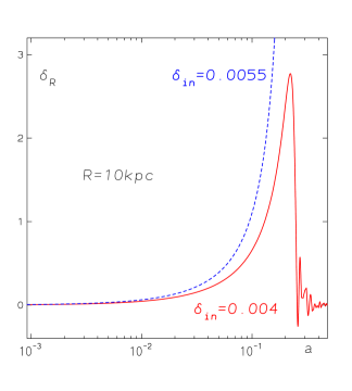
Figure 1: Evolution of $\delta_{R}(a)$ in the tachyon spherical model from $a_{\rm dec}=1/1090$ for $n=2$, $R$ = 10 kpc, $\delta_{R}(a_{\rm dec})$ =0.004 (solid) and $\delta_{R}(a_{\rm dec})$ =0.0055 (dashed).

In figure 1 the representative case of evolution of two initial perturbations starting from decoupling for $R$ = 10 kpc is shown for $n=2$. The plots represent two distinct regimes: the growing mode or condensation (blue dashed line) and the damped oscillations (red solid line). In contrast to the linear theory, where for any $R$ the acoustic horizon will eventually stop $\delta_{R}$ from growing, irrespective of the initial value of the perturbation, here we have for an initial $\delta_{R}(a_{\rm dec})$ above a certain threshold $\delta_{c}(R)$, $\delta_{R}(a)\rightarrow\infty$ at finite $a$, just as in the dust model. Thus perturbations with $\delta_{R}(a_{dec})\geq\delta_{c}(R)$ evolve into a nonlinear gravitational condensate that at low $z$ behaves as pressureless super-particles. Conversely, for a sufficiently small $\delta_{R}(a_{\rm dec})$, the acoustic horizon can stop $\delta_{R}(a)$ from growing; at low redshift the perturbations behave as expected from linear theory. Figure 2 shows how the threshold $\delta_{c}(R)$ divides the two regimes depending on the comoving scale $R$.

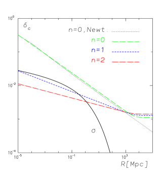
Figure 2: Initial value $\delta_{R}(a_{\rm dec})$ versus $R$ for $\Omega=0.27$ and $h=0.71$. The threshold $\delta_{c}(R)$ is shown by the line separating the condensation regime from the damped oscillations regime. The solid line gives $\sigma(R)$ calculated using the concordance model.

The crucial question now is what fraction of the tachyon gas goes into condensate. In [31] it was shown that if this fraction was sufficiently large, the CMB and the mass power spectrum could be reproduced for the simple Chaplygin gas. To answer this question quantitatively, we follow the Press-Schechter procedure [58] as in [38]. Assuming $\delta_{R}(a_{\rm dec})$ is given by a Gaussian random field with dispersion $\sigma(R)$, and including the notorious factor of 2, to account for the cloud in cloud problem, the condensate fraction at a scale $R$ is given by

$$F(R)=2\int_{\delta_{c}(R)}^{\infty}\;\frac{d\delta}{\sqrt{2\pi}\sigma(R)}\;{\rm exp}\left(-\frac{\delta^{2}}{2\sigma^{2}(R)}\right)={\rm erfc}\left(\frac{\delta_{c}(R)}{\sqrt{2}\;\sigma(R)}\right)\,,$$ (71)

where $\delta_{c}(R)$ is the threshold shown in figure 2. In figure 2 we also exhibit the dispersion

$$\sigma^{2}(R)=\int_{0}^{\infty}\;\frac{dk}{k}\;{\rm exp}(-k^{2}R^{2})\Delta^{2}(k,a_{\rm dec}),$$ (72)

calculated using the Gaussian window function and the variance of the concordance model [3]

$$\Delta^{2}(k,a)={\rm const}\left(\frac{k}{aH}\right)^{4}T^{2}(k)\left(\frac{k}{7.5a_{0}H_{0}}\right)^{n_{s}-1}\,.$$ (73)

In figure 3 we present $F(R)$, calculated using (71)-(73) with const=7.11$\times 10^{-9}$, the spectral index $n_{s}$=1.02, and the parameterization of Bardeen et al [59] for the transfer function $T(k)$ with $\Omega_{B}$=0.04. The parameters are fixed by fitting (73) to the 2dFGRS power spectrum data [60]. Our result demonstrates that the collapse fraction is about 70% for $n=2$ for a wide range of the comoving size $R$ and peaks at about 45% for $n=1$.

Albeit encouraging, these preliminary results do not in themselves demonstrate that the tachyon with potential (8) constitutes a viable cosmology. Such a step requires the inclusion of baryons and comparison with the full cosmological data, much of which obtains at low redshift. What has been shown is that it is not valid in an adiabatic model to simply pursue linear perturbations to the original background : the system evolves nonlinearly into a mixed system of gravitational condensate and residual k-essence so that the “background” at low $z$ is quite different from the initial one. Because of this one needs new computational tools for a meaningful confrontation with the data.

Figure 3: Fraction of the tachyon gas in collapsed objects using $\delta_{c}(R)$ and $\sigma(R)$ from figure 2.

5 Summary and Conclusions

The first key test for any proposed quartessence model should be: Does it actually yield nonlinear dark matter structure, as well as linear dark energy in the inhomogeneous almost FRW universe that we see. In this paper we have analyzed the nonlinear evolution of the tachyon-like k-essence with a very simple potential $V=V_{0}\varphi^{2n}$. We have demonstrated that a significant fraction of the fluid, in particular for $n=2$, collapses into condensate objects that play the role of cold dark matter. No dimensionless fine tunings were required beyond the inevitable $\sqrt{G}H_{0}\ll 1$.

Moreover, these results were obtained in a relativistic framework for nonlinear evolution that is as simple as the spherical dust model but includes the key effects of the acoustic horizon. Although it could be subject to possible improvements (e.g. a variable Gaussian width [38], and it is lacking the sophistication of the exact spherical model, [61], it does allow us to make the sort of quantitative assessments that have been missing [62]. It is directly formulated in a convenient coordinate gauge, does not involve any hidden assumptions, and it easily deals with multi-component systems.

The tachyon k-essence unification remains to be tested against large-scale structure and CMB observations. However, we maintain, contrary to the opinion advocated in [21], that the sound speed problem may be alleviated in unified models no more unnatural than the $\Lambda$CDM model. Indeed, an encouraging feature of the positive power-law potential is that it provides for acceleration as a periodic transient phenomenon [63] which obviates the de Sitter horizon problem [41] , and, we speculate, could even be linked to inflation.

Appendix A Adiabatic speed of sound

The standard definition of the adiabatic speed of sound is

$$c_{s}^{2}=\left.\frac{\partial p}{\partial\rho}\right|_{s/n}\;\;,$$ (74)

where the differentiation is taken at constant $s/n$, i.e. for an isentropic process. Here $s=S/V$ is the entropy density and $n=N/V$ the particle number density associated with the particle number $N$. We use the terminology and notation of Landau and Lifshitz [64] (see also [65])). For a general k-essence, with ${\cal L}={\cal L}(\varphi,X)$, equation (74) may be written as

$$c_{s}^{2}=\left.\frac{dp}{d\rho}\right|_{s/n}=\left.\frac{(\partial p/\partial X)dX+(\partial p/\partial\varphi)d\varphi}{(\partial\rho/\partial X)dX+(\partial\rho/\partial\varphi)d\varphi}\right|_{s/n}\;\;,$$ (75)

where the differentials $dX$ and $d\varphi$ are subject to the constraint $d(s/n)=0$. Next we show that this constraint implies $d\varphi=0$.

We start from the standard thermodynamical relation

$$d(\rho V)=TdS-p\,dV,$$ (76)

where the volume is, up to a constant factor, given by $V=1/n$. Equation (76) may then be written in the form

$$dh=Td\left(\frac{s}{n}\right)+\frac{1}{n}dp\;\;,$$ (77)

where

$$h=\frac{p+\rho}{n}$$ (78)

is the enthalpy per particle. For an isentropic relativistic flow one can define a flow potential $\varphi$ such that [64]

$$hu_{\mu}=\varphi_{,\mu}\,.$$ (79)

Comparing this with (11) we find

$$h=\sqrt{X}\,.$$ (80)

This together with (12) and (13) yields in turn

$$n=2\sqrt{X}{\cal L}_{X}\,.$$ (81)

This expression for the particle number density is derived for an isentropic process. In a purely kinetic k-essence with ${\cal L}={\cal L}(X)$, equation (81) follows from the field equation for $\varphi$

$$({\cal L}_{X}g^{\mu\nu}\varphi_{,\mu})_{;\nu}=0\,,$$ (82)

which implies conservation of the current

$$j_{\mu}=2{\cal L}_{X}\varphi_{,\mu}=nu_{\mu}\,.$$ (83)

The particle number density $n$ in this expression coincides with (81). However, in a general k-essence, with ${\cal L}={\cal L}(\varphi,X)$, the field equation (18) does not imply that the current (83) is conserved. Nevertheless, equation (81) is still a valid expression for a conserved particle number density when the condition $d(s/n)=0$ is imposed.

From (77) with $d(s/n)=0$ and using (80) we obtain

$$dp=n\,dh=\frac{n}{2\sqrt{X}}dX.$$ (84)

Comparing this with the general expression for the total differential of $p$

$$dp=\frac{\partial p}{\partial X}dX+\frac{\partial p}{\partial\varphi}d\varphi$$ (85)

we must have $d\varphi=0$ and

$$\frac{\partial p}{\partial X}=\frac{n}{2\sqrt{X}}={\cal L}_{X}\,,$$ (86)

as it should be. Hence, we conclude that an isentropic process implies $d\varphi=0$ and equation (75) yields

$$c_{s}^{2}=\left.\frac{\partial p}{\partial\rho}\right|_{\varphi}=\frac{\partial p/\partial X}{\partial\rho/\partial X}\,.$$ (87)

Appendix B Braneworld Connection

It is useful to view the tachyon condensate from the braneworld perspective. Consider a 3+1 brane moving in a 4+1 bulk spacetime with metric

$$ds_{5}^{2}=g_{(5)MN}dX^{M}dX^{N}=f(y)^{2}g_{\mu\nu}(x)dx^{\mu}dx^{\nu}-dy^{2}$$ (88)

where we generalize [9, 10, 43] to allow for a warping of the constant $y$ slices through $f(y)$. The points on the brane are parameterized by $X^{\mu}(x^{\mu})$, and $G_{\mu\nu}=g_{(5)MN}X_{,\mu}^{M}X_{,\nu}^{N}$ is the induced metric. Taking the Gaussian normal parameterization $X^{M}=\left(x^{\mu},Y(x^{\mu})\right)$, we have

$$G_{\mu\nu}=f(Y)^{2}g_{\mu\nu}(x)-Y_{,\mu}Y_{,\nu}\,.$$ (89)

The Dirac-Born-Infeld action for the brane is

$$S_{\rm brane}=-\sigma\int d^{4}x\sqrt{-\det G_{\mu\nu}}=-\sigma\int d^{4}x\sqrt{-g}\,f(Y)^{4}\left[1-\frac{g^{\mu\nu}Y_{,\mu}Y_{,\nu}}{f^{2}(Y)}\right]^{1/2},$$ (90)

and with the redefinitions

$$\frac{Y_{,\mu}}{f(Y)}=\varphi_{,\mu}\>,\hskip 42.67912pt\sigma f(Y)^{4}=V(\varphi)$$ (91)

we obtain

$${\cal{L}}_{\rm brane}=-V(\varphi)\sqrt{1-g^{\mu\nu}\varphi_{,\mu}\varphi_{,\nu}}\,.$$ (92)

For an unwarped bulk we obtain $f=1$ and $V=\sigma=\sqrt{A}$, i.e. the simple Chaplygin gas. In general, $V(\varphi)$ identifies ${\cal{L}}_{\rm brane}$ with the tachyon model. If the brane also couples to, e.g., bulk form fields, there are additional terms that are functions of $\varphi$ only. Thus every tachyon condensate model can be interpreted as a 3+1 brane moving in a 4+1 bulk. Note that this is true only for (92) or (52) but not for (51). The prescription (89) does not take into account the distortion of the bulk metric when the brane is not flat. This, however, can be accounted for using the methods of [66].

Given $V(\varphi)$ the warp factor can be reconstructed via

$$Y-Y_{0}=\int f(Y(\varphi))d\varphi=\sigma^{-1/4}\int V(\varphi)^{1/4}d\varphi.$$ (93)

For example, for the power-law potential

$$V(\varphi)=V_{0}\varphi^{2n}\;\;,$$ (94)

we obtain

$$f(Y)=\left(\frac{Y-Y_{0}}{l}\right)^{n/(2+n)},\hskip 42.67912ptl=\frac{2}{n+2}\left(\frac{\sigma}{V_{0}}\right)^{1/(2n)}\;\;.$$ (95)

Using (67) and writing $\sqrt{G\sigma}=\epsilon/l$, one finds $\epsilon\sim(lH_{0})^{1+n}$ which is the only fine tuning for $n\neq-1$ and a small-scale extra dimension.

References

- [1] S. Perlmutter et al. Astrophys. J. 517, 565 (1999); A.G. Riess et al. Astron. J. 116, 1009 (1998).
- [2] N.W. Halverson et al. Astrophys. J. 568, 38 (2000); C.B. Netterfield et al. Astrophys. J. 571, 604 (2002).
- [3] G. Hinshaw et al. Astrophys. J. Suppl. 170, 288 (2007); [arXiv: astro-ph/0603451]; D.N. Spergel et al. Astrophys. J. Suppl. 170, 377 (2007); [arXiv: astro-ph/0603449]; E. Komatsu et al. submitted to Astrophys. J. Suppl.; [arXiv: 0803.0547].
- [4] P.J.E. Peebles and B. Ratra, Rev. Mod. Phys. 75, 599 (2003).
- [5] V. Sahni, Lect. Notes Phys. 653, 141 (2004); [arXiv: astro-ph/0403324] ; E.J. Copeland, M. Sami, and S. Tsujikawa, Int. J. Mod. Phys. 15, 1753 (2006).
- [6] W. Hu, Astrophys. J. 506, 485 (1998).
- [7] A. Kamenshchik, U Moschella, and V. Pasquier, Phys. Lett. B 511, 265 (2001).
- [8] N. Bilić, G.B. Tupper, and R.D. Viollier, Phys. Lett. B 535, 17 (2002).
- [9] N. Bilić, G.B. Tupper, and R.D. Viollier, in Proceedings of the International Conference on Matter in Astro- and Particle Physics, DARK 2002, edited by H.V. Klapdor-Kleingrothaus and R.D. Viollier (Berlin, Heidelberg:Springer-Verlag), Int. Conf. B 535, 17 (2002); [arXiv:astro-ph/0207423].
- [10] R. Jackiw, Lectures on fluid dynamics. A Particle theorist’s view of supersymmetric, non-Abelian, noncommutative fluid mechanics and d-branes (New-York: Springer-Verlag) (2002).
- [11] M. Makler, S.Q. de Oliveira, and I. Waga, Phys. Lett. B 555, 1 (2003).
- [12] R.R.R. Reis, M. Makler, and I. Waga, Phys. Rev. D 69, 101301 (2004).
- [13] L.P. Chimento, Phys. Rev. D 69, 123517 (2004).
- [14] R.J. Scherrer, Phys. Rev. Lett. 93, 011301 (2004).
- [15] C. Armendariz-Picon, T. Damour, and V. Mukhanov, Phys. Lett. B 458, 209 (1999).
- [16] J. Polchinski, String Theory (Cambridge U Press, Cambridge) (1998).
- [17] R. Sundrum, Phys. Rev D 59, 085009 (1999).
- [18] Ya. B. Zel’dovich, Astron. Astrophys. 5, 8 (1970).
- [19] J.C. Fabris, S.V.B. Gonçalves, and P.E. de Souza, Gen. Relativ. Gravit. 34, 53 (2002); J.C. Fabris, S.V.B. Gonçalves, and P.E. de Souza, Gen. Relativ. Gravit. 34, 2111 (2002).
- [20] V. Gorini, A.Y. Kamenshchik, U. Moschella, O.F. Piattella, and A.A. Starobinsky, JCAP 0802, 016 (2008).
- [21] H.B. Sandvik, M. Tegmark, M. Zaldarriaga, and I. Waga, Phys. Rev. D 69, 123524 (2004).
- [22] P. Carturan and F. Finelli, Phys. Rev. D 68, 103501 (2003).
- [23] A. Dev, J.S. Alcaniz, and D. Jain, Phys. Rev. D 67, 023515 (2003).
- [24] A. Dev, D. Jain, and J.S. Alcaniz, Astron. Astrophys. 417, 847 (2004).
- [25] P.P. Avelino, L.M.G. Beça, J.P.M. de Carvalho, C.J.A.P. Martins, and P. Pinto, Phys. Rev. D 67, 023511 (2003).
- [26] J.S. Alcaniz, D. Jain, and A. Dev, Phys. Rev. D 67 043514 (2003).
- [27] R. Bean and O. Doré, Phys. Rev. D 68 023515 (2003).
- [28] L. Amendola, F. Finelli, C. Burigana, and D. Carturan, JCAP 0307, 005 (2003).
- [29] T. Multamäki, M. Manera, and E. Gaztañaga, Phys. Rev. D 69, 023004 (2004).
- [30] O. Bertolami, A.A. Sen, S. Sen, and P.T. Silva, MNRAS 353, 329 (2004).
- [31] N. Bilić, R.J. Lindebaum, G.B. Tupper, and R.D. Viollier, in Proceedings of the XVth Rencontres de Blois International Conference on Physical Cosmology, France, 2003, edited by J. Dumarchez, et al. (Vietnam: The Gioi Publishers) (2005); [arXiv: astro-ph/0310181].
- [32] M.C. Bento, O. Bertolami, and A.A. Sen, Phys. Rev. D 66, 043507 (2002).
- [33] O. Bertolami, Preprint (2004) [arXiv: astro-ph/0403310].
- [34] G.F.R. Ellis, R. Maartens, and M.A.H. MacCallum, Gen. Relativ. Gravit. 39, 1651 (2007).
- [35] J.P. Bruneton, Phys. Rev. D 75, 085013 (2007).
- [36] J.U. Kang, V. Vanchurin, and S. Winitzki, Phys. Rev. D 76, 083511 (2007).
- [37] E. Babichev, V. Mukhanov, and A. Vikman, JHEP 0802, 101 (2008).
- [38] N. Bilić, R.J. Lindebaum, G.B. Tupper, and R.D. Viollier, JCAP 0411, 008 (2003); [arXiv: astro-ph/0307214].
- [39] E. Gaztãnaga and J.A. Lobo, Astrophys. J. 548, 47 (2001).
- [40] R.R.R. Reis, I. Waga, M.O. Calvão, and S.E. Jorás, Phys. Rev. D 68, 061302 (2003); R.R.R. Reis, M. Makler, and I. Waga, Phys. Rev. D 69, 101301 (2004); M. Makler, S.Q. de Oliviera, and I. Waga, Phys. Rev. D 68, 123521 (2003).
- [41] N. Bilić, G.B. Tupper, and R.D. Viollier, JCAP 0510, 003 (2005); [arXiv: astro-ph/0503428].
- [42] N. Bilić, G.B. Tupper, and R.D. Viollier, Preprint (2005) [arXiv: hep-th/0504082].
- [43] N. Bilić, G.B. Tupper, and R.D. Viollier, J. Phys. A40, 6877 (2007); [arXiv: gr-qc/0610104].
- [44] A. Sen, Mod. Phys. Lett. A17, 1797 (2002); A. Sen, J. High Energy Phys. JHEP 0204, 048 (2002); A. Sen, J. High Energy Phys. JHEP 0207, 065 (2002).
- [45] G.W. Gibbons, Class. Quant. Grav. 20, S321 (2003).
- [46] T. Padmanabhan and Choudhury T. Roy, Phys. Rev. D 66, 081301 (2002).
- [47] Z.-K. Guo and Y.-Z. Zhang, Phys. Lett. B 645, 326 (2007).
- [48] D. Bertacca, S. Matarrese, and M. Pietroni, Mod. Phys. Lett. A22, 2893 (2007).
- [49] D. Bertacca, N. Bartolo, A. Diafero, and S. Matarrese, Preprint (2008) [arXiv: 0807.1020].
- [50] L.R. Abramo, R.C. Batista, L. Liberato, and R. Rosenfeld, JCAP 0711 012, (2007).
- [51] J. Garriga and V.F. Makhanov, Phys. Lett. B 458, 219 (1999).
- [52] S.D.H. Hsu, A. Jenkins, and M.B. Wise, Phys. Lett. B 597, 270 (2004); N. Bilic, G.B. Tupper, and R.D. Viollier, JCAP 0809, 002 (2008); [arXiv: 0801.3942].
- [53] C. Bonvin, C. Caprini, and R. Durrer, Phys. Rev. Lett. 97, 081303 (2006).
- [54] N. Bilić, Class. Quant. Grav. 16, 3953 (1999); [arXiv: gr-qc/9908002].
- [55] W.K. Kolb, V. Marra, and S. Matarrese (2008) [arXiv: 0807.0401].
- [56] A.R. Liddle and D.H. Lyth, Cosmological Inflation and Large Scale Structure (Cambridge U Press, Cambridge) (2000).
- [57] V.F. Mukhanov, H.A. Feldman, and R.H. Brandenberger, Phys. Rep. 115, 203 (1992).
- [58] W.H. Press and P. Schechter, Astrophys. J. 187, 425 (1974).
- [59] J.M. Bardeen, J.R. Bond, N. Kaiser, and A.S. Szalay, Astrophys. J. 304, 15 (1986).
- [60] W.J. Percival et al., Mon. Not. R. Astron. Soc. 327, 1297 (2001).
- [61] R.A. Sussman, Preprint (2008) [arXiv: 0801.3324].
- [62] P.P. Avelino, L.M.G. Beca, and C.J.A.P. Martins, Phys. Rev. D 77, 063515 (2008).
- [63] A. Frolov, L. Kofman, and A. Starobinsky, Phys. Lett. B 545, 8 (2002).
- [64] L.D. Landau, E.M. Lifshitz, Fluid Mechanics, Pergamon, Oxford (1993).
- [65] C.G. Tsagas, A. Challinor, and R. Maartens, Phys. Rep. 465, 61 (2008); [arXiv: 0705.4397].
- [66] J.E. Kim, G.B. Tupper, and R.D. Viollier, Phys. Lett. B 593, 209 (2004); J.E. Kim, G.B. Tupper, and R.D. Viollier, Phys. Lett. B 612, 293 (2005).