Stable magnetic equilibria and their evolution in the
upper main sequence, white dwarfs, and neutron stars

Abstract

Context. Long-lived, large-scale magnetic field configurations exist in upper main sequence, white dwarf, and neutron stars. Externally, these fields have a strong dipolar component, while their internal structure and evolution are uncertain but highly relevant to several problems in stellar and high-energy astrophysics.

Aims. We discuss the main properties expected for the stable magnetic configurations in these stars from physical arguments and the ways these properties may determine the modes of decay of these configurations.

Methods. We explain and emphasize the likely importance of the non-barotropic, stable stratification of matter in all these stars (due to entropy gradients in main-sequence envelopes and white dwarfs, due to composition gradients in neutron stars). We first illustrate it in a toy model involving a single, azimuthal magnetic flux tube. We then discuss the effect of stable stratification or its absence on more general configurations, such as axisymmetric equilibria involving poloidal and toroidal field components. We argue that the main mode of decay for these configurations are processes that lift the constraints set by stable stratification, such as heat diffusion in main-sequence envelopes and white dwarfs, and beta decays or particle diffusion in neutron stars. We estimate the time scales for these processes, as well as their interplay with the cooling processes in the case of neutron stars.

Results. Stable magneto-hydrostatic equilibria appear to exist in stars whenever the matter in their interior is stably stratified (not barotropic). These equilibria are not force-free and not required to satisfy the Grad-Shafranov equation, but they do involve both toroidal and poloidal field components. In main sequence stars with radiative envelopes and in white dwarfs, heat diffusion is not fast enough to make these equilibria evolve over the stellar lifetime. In neutron stars, a strong enough field might decay by overcoming the compositional stratification through beta decays (at the highest field strengths) or through ambipolar diffusion (for somewhat weaker fields). These processes convert magnetic energy to thermal energy, and they occur at significant rates only once the latter is less than the former; therefore, they substantially delay the cooling of the neutron star, while slowly decreasing its magnetic energy.

1 Introduction

Upper main sequence stars, white dwarfs, and neutron stars appear to have long-lived magnetic fields. These fields are organized on large scales, in the sense that the dipole field components (and perhaps some other, low-order multipoles; e. g. Bagnulo et al. 1999, 2000) are not much weaker than the rms surface field, unlike the highly chaotic field of the Sun.

The highest detected (surface dipole) magnetic field strengths are $B_{\mathrm{max}}\sim 10^{3}\leavevmode\nobreak\ \mathrm{G}$ in O stars (radius $R\sim 10\leavevmode\nobreak\ R_{\sun}$; Donati et al. 2002, 2006; Petit et al. 2008), $B_{\mathrm{max}}\sim 3\times 10^{4}\leavevmode\nobreak\ \mathrm{G}$ in chemicallly peculiar A and B stars (Ap/Bp stars, $R\sim 3\leavevmode\nobreak\ R_{\sun}$; Mathys et al. 1997; Bagnulo et al. 1999), $B_{\mathrm{max}}\sim 10^{9}\leavevmode\nobreak\ \mathrm{G}$ in white dwarfs ($R\sim 10^{4}\mathrm{km}$; Schmidt et al. 2003), and $B_{\mathrm{max}}\sim 10^{15}\leavevmode\nobreak\ \mathrm{G}$ in “magnetars”, a subclass of strongly magnetized neutron stars ($R\sim 10\leavevmode\nobreak\ \mathrm{km}$; Kouveliotou et al. 1998; Woods et al. 1999), in all cases yielding very similar total magnetic fluxes, $\Phi_{\mathrm{max}}=\pi R^{2}B_{\mathrm{max}}\sim 10^{27.5}\leavevmode\nobreak\ \mathrm{G\leavevmode\nobreak\ cm^{2}}$. This coincidence has often been interpreted as an argument for flux freezing during stellar evolution (Ruderman, 1972; Reisenegger, 2001b, 2003; Ferrario & Wickramasinghe, 2005a, b, 2006), although its feasibility has been called into question (Thompson & Duncan, 1993; Spruit, 2008). Of course, a large fraction of the original magnetic flux might be ejected with the stellar envelope. On the other hand, substantial field amplification through differential rotation, convection, and various instabilities could plausibly occur in proto-neutron stars if they are born rapidly rotating (Thompson & Duncan, 1993; Spruit, 2002, 2008).

Connected to the similar fluxes is that these stars also have similar ratios of fluid pressure ($P\sim GM^{2}/R^{4}$, where $G$ is the gravitational constant and $M$ is the mass of the star) to magnetic pressure ($B^{2}/8\pi$),

$$\beta={8\pi P\over B^{2}}\sim{8\pi^{3}GM^{2}\over\Phi^{2}}\sim 3\times 10^{6}\left(M\over M_{\sun}\right)^{2}\left(\Phi\over\Phi_{\mathrm{max}}\right)^{-2},$$ (1)

a large number, even for the most highly magnetized objects, implying that the magnetic field causes only very minor perturbations to their hydrostatic equilibrium structure.

Another similarity among these stars is that much or all of their structure is stably stratified, i. e. stable to convection. The radiative envelopes of upper main sequence stars, as well as the whole interior of white dwarfs, are stabilized by the radially increasing specific entropy $s$, while in neutron stars the same effect is caused by a radially varying mix of different particle species (Pethick, 1992; Reisenegger & Goldreich, 1992; Reisenegger, 2001a), which in the outer core reduces to a radially varying proton and electron fraction, $Y\equiv n_{p}/(n_{n}+n_{p})=n_{e}/(n_{n}+n_{p})$, where $n_{i}$ stands for the number densities of neutrons ($i=n$), protons ($i=p$) and electrons ($i=e$).

The structure of the magnetic field inside these stars is not known, although it is highly relevant to their evolution:

• It affects the radial transport of angular momentum and chemical elements (e. g. Heger et al. 2005);

• it is plausibly the dominant source of energy for both the outbursts and the persistent emission of soft gamma repeaters (SGRs) and anomalous X-ray pulsars (AXPs), for this reason collectively called “magnetars” (Thompson & Duncan, 1993, 1996);

• it is likely to play an important role in the frequency spectrum of quasi-periodic oscillations observed after SGR flares (Levin, 2007);

• it leads to slight deformations of neutron stars that could give rise to precession of pulsars (Wasserman, 2003) and to the emission of gravitational waves (Cutler, 2002).

Magnetohydrodynamic (MHD) simulations of stably stratified stars with random initial magnetic field configurations have shown them to evolve on Alfvén-like time scales into long-lived structures whose further evolution and decay appears to be controlled by dissipative processes (in the simulations, Ohmic diffusion; Braithwaite & Spruit 2004, 2006; Braithwaite & Nordlund 2006). Often, but not always (Braithwaite, 2008), these are roughly axisymmetric combinations of linked poloidal and toroidal components, whose external appearance is essentially dipolar. It appears plausible that these configurations approximate the true magnetic field structures in upper main sequence stars, white dwarfs, and neutron stars.

In § 2, we present arguments to the effect that the stable stratification of the stellar matter should be an essential ingredient to these equilibria. This means that, contrary to assumptions in the recent literature (e. g. Pérez-Azorín et al. 2006; Broderick & Narayan 2008; Mastrano & Melatos 2008), these are definitely not force-free fields. In fact, it is shown in Appendix A that there are no true force-free equilibria in stars, while those proposed in the literature actually have singular magnetic forces on the stellar surface. Moreover, the fluid cannot be treated as barotropic, therefore the field components are not required to satisfy the Grad-Shafranov equation (Mestel, 1956), contrary to the popular belief (Tomimura & Eriguchi, 2005; Yoshida et al., 2006; Haskell et al., 2008; Akgün & Wasserman, 2008; Kiuchi & Kotake, 2008). In fact, the range of available equilibria becomes much wider in a stably stratified, non-barotropic fluid. The constraints imposed by the stability of these equilibria are far from obvious, but we argue that there are probably no equilibria in barotropic stars, while it is likely that there are equilibria with linked toroidal and poloidal fields in stably stratified stars.

Of course, the specific entropy $s$ and the proton fraction $Y$ are not perfectly conserved quantities within each fluid element, but can be changed by dissipative processes, discussed in § 3: In the case of $s$, through heat diffusion (Parker, 1974), in the case of $Y$, by (direct or inverse) beta decays or by ambipolar diffusion (motion of charged relative to neutral particles; Pethick 1992; Goldreich & Reisenegger 1992; Thompson & Duncan 1996; Hoyos et al. 2008). Thus, the condition of stable stratification, and with it the hypothetically associated stable magnetic equilibrium configuration, although excellent approximations on short (Alfvén-like) time scales, are eroded on the time scales of the dissipative processes mentioned above, leading to the decay of these structures (Goldreich & Reisenegger, 1992), and perhaps to a sudden loss of stability (Braithwaite & Spruit, 2004, 2006; Braithwaite & Nordlund, 2006). In main-sequence stars, white dwarfs, and weakly magnetized neutron stars, these appear to be too long to act on the stellar life time, but in strongly magnetized neutron stars their time scales become shorter, so they might plausibly drive magnetic field decay, leading to internal heating and to the magnetar phenomenon (Thompson & Duncan, 1996; Arras et al., 2004).

In principle, the Hall drift might also play a role in the field evolution in neutron stars (Jones, 1988; Urpin & Shalybkov, 1991; Goldreich & Reisenegger, 1992; Reisenegger et al., 2005, 2007; Pons & Geppert, 2007). However, its time scale in neutron star cores tends to be somewhat longer than those of the other processes considered here (Goldreich & Reisenegger, 1992). Moreover, in an axially symmetric, equilibrium magnetic field configuration, the effect of the Hall drift is exactly cancelled by bulk fluid motions (Reisenegger & Thompson, 2009), so we do not take it into account. For simplicity, we also refrain from discussing the role of the solid crust of the neutron star, as well as the effects of superconductivity and superfluidity, which alter the magnetic stresses (Easson & Pethick, 1977; Akgün & Wasserman, 2008) as well as the dissipative processes. We also ignore the process of initial set-up of the magnetic equilibrium, which might be a highly dynamical process involving differential rotation and possibly a dynamo (Thompson & Duncan, 1993; Spruit, 2002), but concentrate on the properties imposed by the equilibrium and stability conditions and on the long-term evolution of the field.

A concise summary of our conclusions is given in § 4. Parts of this discussion have already been given elsewhere (Reisenegger, 2007, 2008).

2 Magnetic equilibria and stable stratification

2.1 Force balance

In a conducting, fluid star, a general MHD equilibrium is set by the condition that the net force on the fluid vanishes everywhere, i. e.

$${\bf f}_{B}+{\bf f}_{F}=0,$$ (2)

where

$${\bf f}_{B}\equiv{1\over c}{\bf j}\times{\bf B}$$ (3)

is the magnetic (Lorentz) force per unit volume, written in terms of the magnetic field, ${\bf B}$, and its associated current density, ${\bf j}=(c/4\pi)\nabla\times{\bf B}$, and

$${\bf f}_{F}\equiv-\nabla P-\rho\nabla\psi$$ (4)

is the fluid force, which depends on its pressure, $P$, density $\rho$, and gravitational potential, $\psi$.

In all the stars of interest, the fluid is non-barotropic, i. e. the density is not a function of pressure only, but depends on an additional, non-trivial variable $X$, which is conserved on dynamical (sound or Alfvén wave crossing) time scales: specific entropy ($X=s$) in the case of upper main sequence stars and white dwarfs, and the fraction of protons ($X=Y$) or other minor constituent particles required by beta equilibrium in the case of neutron stars (Pethick, 1992; Reisenegger & Goldreich, 1992).

As shown in equation (1), the fluid pressure is much higher than the magnetic pressure, so we take the point of view that the magnetic forces create only a slight perturbation to the background hydrostatic equilibrium state (${\bf f}_{F}=0$) the star would have in their absence. In addition, we invoke the standard Cowling approximation of neglecting perturbations to the gravitational potential, also used in the simulations of Braithwaite and collaborators.

We do not assume that the unperturbed star is spherically symmetric, so our arguments can also be applied to stars that are uniformly rotating, in which case $\psi$ has to be interpreted as the effective potential, also including centrifugal effects. However, we ignore the effects of meridional circulation. The time scale for this process, due to the interaction of stellar rotation and internal heat flow, is $t_{\mathrm{circ}}\sim(\Omega_{K}/\Omega)^{2}t_{\mathrm{KH}}$, where $\Omega$ is the stellar rotation rate, $\Omega_{K}$ is its maximum (Keplerian or “break-up”) value, and $t_{\mathrm{KH}}$ is the (Kelvin-Helmholtz) time scale required to radiate away the thermal energy content of the star. For main sequence stars, $t_{\mathrm{KH}}$ is substantially shorter than their main-sequence life time, so meridional circulation can modify the magnetic field structure of sufficiently fast rotators, $P=2\pi/\Omega<5\mathrm{d}$ (Moss, 1984, 1990; Mestel, 1999), to which our analysis will therefore not apply. For white dwarfs, $t_{\mathrm{KH}}$ is their cooling time, i. e. essentially their age, so meridional circulation is unimportant unless they rotate near break-up (Tassoul & Tassoul, 1983). In none of these cases, the magnetic field is expected to be strong enough to have a substantial influence on the pattern or time scale of meridional circulation. For neutron stars, since the main source of stratification is not entropy but chemical composition (Reisenegger & Goldreich, 1992), meridional circulation will not occur at all.

Thus, we write the fluid force in terms of the Eulerian perturbations (changes at fixed spatial positions) of density and pressure, $\delta\rho$ and $\delta P$, respectively, as

$${\bf f}_{F}=-\nabla\delta P-\delta\rho\nabla\psi.$$ (5)

The perturbations can be viewed as being produced by a displacement field $\xi$, which allows us to introduce Lagrangian perturbations (comparing the variables in the same fluid element as it gets displaced) $\Delta\rho$, $\Delta P$, formally related to the Eulerian perturbations by

$$\Delta\equiv\delta+\mbox{\boldmath$\xi$}\cdot\nabla,$$ (6)

where the gradient operator acts on the corresponding unperturbed “background” quantity, $\rho_{b}$ or $P_{b}$.

If the displacement is fast enough, it can be taken to conserve specific entropy and chemical composition, so the Lagrangian perturbations are related by the adiabatic index

$$\gamma_{p}\equiv{\Delta\ln P\over\Delta\ln\rho}=\left(\partial\ln P\over\partial\ln\rho\right)_{X},$$ (7)

which is generally different from the analogous quantity characterizing the hydrostatic equilibrium profile of the star,

$$\gamma_{b}\equiv{d\ln P_{b}\over d\ln\rho_{b}}=\left(\partial\ln P\over\partial\ln\rho\right)_{X}+\left(\partial\ln P\over\partial\ln X\right)_{\rho}{d\ln X\over d\ln\rho_{b}}.$$ (8)

Then, also using the condition of mass conservation, $\Delta\rho=-\rho_{b}\nabla\cdot\mbox{\boldmath$\xi$}$, equation (5) can be manipulated into the form

$${\bf f}_{F}=-\rho_{b}\nabla\left(\delta P\over\rho_{b}\right)+\left({\gamma_{p}\over\gamma_{b}}-1\right)\Delta\rho\nabla\psi,$$ (9)

where the first term would be present as well in a barotropic, homogeneous fluid, whereas the second accounts for buoyancy effects. The latter is stabilizing if $\gamma_{p}>\gamma_{b}$ and destabilizing in the opposite case.

In upper main sequence stars, the fluid is a classical, monatomic ideal gas with $\gamma_{p}=5/3$, with their radiative envelopes well described by $\gamma_{b}\approx 4/3$ (MacGregor & Cassinelli, 2003), so $\gamma_{p}/\gamma_{b}-1\approx 1/4$. In white dwarfs, the electrons are highly degenerate ($kT\ll E_{Fe}$, where $k$ is Boltzmann’s constant, $T=T_{7}\times 10^{7}\mathrm{K}$ is the interior temperature, and $E_{Fe}$ is the electron Fermi energy, not including the relativistic rest-mass term, $mc^{2}$) and dominate the pressure, but the entropy is contained in the ions, so $\gamma_{p}/\gamma_{b}-1\sim kT/ZE_{F}\sim T_{7}/500$. Finally, in the case of neutron stars, entropy becomes negligible a few seconds after their birth, but they remain stably stratified due to the density-dependent proton fraction, $\gamma_{p}/\gamma_{b}-1\sim Y\sim\mathrm{few}\leavevmode\nobreak\ \%$ (Reisenegger & Goldreich, 1992; Lai, 1994; Reisenegger, 2001a).

Eq. (9) shows that, in a stably stratified fluid (with $\gamma_{p}>\gamma_{b}$), the fluid force has two parts that are determined by two independent, scalar functions, e. g. $\delta P$ and $\Delta\rho$, which give the fluid a greater freedom to balance the magnetic force than it would have in the barotropic case ($\gamma_{p}=\gamma_{b}$). It should be noted that, if the buoyancy term in eq. (9) is crucial to balance a particular field configuration of characteristic length scale comparable to the stellar radius, the characteristic field strength is constrained by

$$|\mathbf{f}_{B}| \sim {B^{2}\over 8\pi R}\sim\left({\gamma_{p}\over\gamma_{b}}-1\right)|\Delta\rho\nabla\psi|$$ (10)

$$\mathrel{\hbox to0.0pt{\lower 4.0pt\hbox{\hskip 1.0pt$\sim$}\hss}\raise 1.0pt\hbox{$<$}} \left({\gamma_{p}\over\gamma_{b}}-1\right)\rho|\nabla\psi|\approx\left({\gamma_{p}\over\gamma_{b}}-1\right)|\nabla P|.$$

Thus, its maximum value is not set by the condition $\beta\mathrel{\hbox to0.0pt{\lower 4.0pt\hbox{$\sim$}\hss}\raise 1.0pt\hbox{$>$}}1$ (with $\beta$ defined in eq. 1), but rather by the more restrictive

$$\beta(\gamma_{p}/\gamma_{b}-1)\mathrel{\hbox to0.0pt{\lower 4.0pt\hbox{$\sim$}\hss}\raise 1.0pt\hbox{$>$}}1,$$ (11)

yielding maximum allowed field strengths of $\sim 10^{8}\leavevmode\nobreak\ \mathrm{G}$ for Ap/Bp stars, $\sim 10^{11}T_{7}^{1/2}\leavevmode\nobreak\ \mathrm{G}$ for white dwarfs, and a few times $10^{17}\leavevmode\nobreak\ \mathrm{G}$ for neutron stars, all of which still substantially exceed the observationally inferred fields in these stars.

2.2 Hierarchy of equilibria and variational principles

Given this physical background, we now explore the more mathematical issue of how magnetic equilibria obtained under progressively more stringent (and, for our purposes, more realistic) constraints can be represented by constrained stationary points of the magnetic energy. We note that, contrary to the previous section, where “perturbations” were deviations from the non-magnetic, hydrostatic equilibrium caused by the magnetic field, here perturbations are taken with respect to successive, magnetic equilibria.

2.2.1 Field-free:

Consider the total magnetic energy within a fixed volume, $U_{B}=\int_{\mathcal{V}}B^{2}d\mathcal{V}/(8\pi).$ The only way to obtain $\delta U_{B}=0$ under a weak, but otherwise arbitrary magnetic field variation is to have $\mathbf{B}=0$ everywhere. This is the absolute minimum of the magnetic energy, and it is eventually obtained in a star placed in vacuum, without external fields, and in which a sufficiently effective dissipation mechanism (such as resistive diffusion) is active.

2.2.2 Current-free:

Of course, $\delta\mathbf{B}$ is not fully arbitrary, but must be divergenceless, so we now consider the slightly more restricted case $\delta\mathbf{B}=\nabla\times\delta\mathbf{A}$. Now,

$$\delta U_{B} = {1\over 4\pi}\int_{\mathcal{V}}\mathbf{B}\cdot\nabla\times\delta\mathbf{A}\leavevmode\nobreak\ d\mathcal{V}$$ (12)

$$= {1\over 4\pi}\left[\int_{\mathcal{V}}\nabla\cdot(\delta\mathbf{A}\times\mathbf{B})\leavevmode\nobreak\ d\mathcal{V}+\int_{\mathcal{V}}\delta\mathbf{A}\cdot\nabla\times\mathbf{B}\leavevmode\nobreak\ d\mathcal{V}\right].$$

In the last result, the first integral can be made to vanish by imposing appropriate boundary conditions on the surface, for example that the magnetic flux through any surface element is fixed (${\mathbf{\hat{n}}}\cdot\delta\mathbf{B}=0$, where ${\mathbf{\hat{n}}}$ is the outward unit normal), which implies that ${\mathbf{\hat{n}}}\times\delta\mathbf{A}=0$. The second term can only be made to vanish for arbitrary $\delta\mathbf{A}$ if the electric current density vanishes everywhere in the volume, $\mathbf{j}=c\nabla\times\mathbf{B}/(4\pi)=0.$ In order to have a finite magnetic field in a volume containing no currents, there must be source currents in some neighboring volume. Therefore, a finite stellar magnetic field cannot be current-free everywhere.

2.2.3 Force-free:

In stars, dissipative processes such as the resistive diffusion of magnetic flux are slow (see § 3 for details) and therefore often negligible. In this context, the only possible perturbations of the magnetic field are those which can be produced by plasma displacements, $\delta\mathbf{A}=\mbox{\boldmath$\xi$}\times\mathbf{B}$, with $\xi$ an arbitrary vector field. In this case, neglecting the divergence term of eq. (12), $\delta U_{B}=-\int_{\mathcal{V}}\leavevmode\nobreak\ \mbox{\boldmath$\xi$}\cdot({\mathbf{j}\times\mathbf{B}/c})\leavevmode\nobreak\ d\mathcal{V}$, so the stationarity of the magnetic energy implies the vanishing of the Lorentz force, ${\mathbf{j}\times\mathbf{B}/c}=0$. This case is relevant in very diffuse plasmas such as those in stellar magnetospheres, where the conductivity is high, but gas pressures and densities are low ($\beta\ll 1$), so the dynamics is dominated by the magnetic field. However, as shown in Appendix A, it is not possible to have magnetic field structures that are force-free everywhere in a star, unless it is confined by (unrealistic) surface forces.

2.2.4 Force balance:

As we saw in § 2.1, the plasma inside stars has $\beta\gg 1$, so the fluid forces, due to pressure and gravity, can by no means be neglected. The total energy perturbation (with respect to some hydrostatic or hydromagnetic equilibrium state) caused by an arbitrary fluid displacement field $\xi$ can be calculated by integrating the work per unit volume $-(1/2)\mathbf{f}\cdot\mbox{\boldmath$\xi$}$ done against the forces of Eqs. (3) and (5) in order to build up this displacement field. In the absence of a magnetic field, the result can be written as

$$\delta U=\int{1\over 2\gamma_{p}P_{b}}\left[\delta P^{2}+\left({\gamma_{p}\over\gamma_{b}}-1\right)(\mbox{\boldmath$\xi$}\cdot\nabla P_{b})^{2}\right]\leavevmode\nobreak\ d\mathcal{V},$$ (13)

where we ignored a surface term that vanishes for appropriate boundary conditions. Clearly, the $\delta P^{2}$ term is always positive, while the other term is positive for a stably stratified fluid ($\gamma_{p}>\gamma_{b}$), zero for a barotropic fluid ($\gamma_{p}=\gamma_{b}$), and negative for a convectively unstable fluid ($\gamma_{p}<\gamma_{b}$). Clearly, there are no unstable (negative-energy) perturbations if $\gamma_{p}\geq\gamma_{b}$. In a stable equilibrium, one must have vanishing Eulerian pressure perturbations, $\delta P=-\gamma_{p}P_{b}\nabla\cdot\mbox{\boldmath$\xi$}-\mbox{\boldmath$\xi$}\cdot\nabla P_{b}=0$, and, if the fluid is stably stratified, also no “vertical” displacements, $\mbox{\boldmath$\xi$}\cdot\nabla P_{b}=0$. All displacements satisfying these conditions produce neutrally stable perturbations. We expect these conditions to still be approximately satisfied in equilibria that involve a weak magnetic field.

When a magnetic field is introduced, the total energy perturbation becomes more complicated,

$$\delta U=\int{\Huge[}{\delta\mathbf{B}^{2}\over 8\pi}-{1\over 2c}\mathbf{j}\cdot\delta\mathbf{B}\times\mbox{\boldmath$\xi$}+\gamma_{p}P(\nabla\cdot\mbox{\boldmath$\xi$})^{2}$$

$$+(\mbox{\boldmath$\xi$}\cdot\nabla P)\nabla\cdot\mbox{\boldmath$\xi$}-(\mbox{\boldmath$\xi$}\cdot\nabla\psi)\nabla\cdot(\rho\mbox{\boldmath$\xi$}){\Huge]}\leavevmode\nobreak\ d\mathcal{V}$$ (14)

(Bernstein et al., 1958), and negative-energy perturbations exist for some field configurations, even if $\gamma_{p}\geq\gamma_{b}$ (Tayler, 1973; Flowers & Ruderman, 1977). However, since these instabilities are caused by the magnetic field, we expect the quantities $|\delta P|$ and (if the fluid is stably stratified) $|\mbox{\boldmath$\xi$}\cdot\nabla P|$ to be small enough to keep the fluid force perturbation $\delta\mathbf{f}_{F}=-\nabla\delta P-\delta\rho\nabla\psi$ not much larger than the magnetic force perturbation $\delta\mathbf{f}_{B}=(\delta\mathbf{j}\times\mathbf{B}+\mathbf{j}\times\delta\mathbf{B})/c$. This requires $|\nabla\cdot(\rho\mbox{\boldmath$\xi$})|\mathrel{\hbox to0.0pt{\lower 4.0pt\hbox{\hskip 1.0pt$\sim$}\hss}\raise 1.0pt\hbox{$<$}}\rho|\mbox{\boldmath$\xi$}|/(\beta\ell)$ for barotropic and stably stratified fluids, and $|\xi_{r}|\mathrel{\hbox to0.0pt{\lower 4.0pt\hbox{\hskip 1.0pt$\sim$}\hss}\raise 1.0pt\hbox{$<$}}|\mbox{\boldmath$\xi$}|/\beta$ only for the latter. Since the non-magnetic terms in Eq. (14) are quadratic in these quantities, they will be smaller than the magnetic terms, therefore it seems reasonable to consider only magnetic energy perturbations, subject to the conditions $\nabla\cdot(\rho\mbox{\boldmath$\xi$})=0$ for barotropic and stably stratified fluids, and additionally $\mbox{\boldmath$\xi$}\cdot\nabla\psi=0$ for the latter. Note that this bypasses some instabilities that originate in particular regions where the fluid forces are weak, such as near the center of the star (Tayler, 1973).

Barotropic fluid:

Thus, for a barotropic fluid with high $\beta$, we impose the constraint $\delta P/\gamma_{p}=\delta\rho=-\nabla\cdot(\rho\mbox{\boldmath$\xi$})=0$, therefore $\mbox{\boldmath$\xi$}=(1/\rho)\nabla\times\mathbf{a}$, where $\mathbf{a}$ is an arbitrary vector field. The magnetic energy perturbation becomes

$$\delta U_{B}=\int_{\mathcal{V}}\leavevmode\nobreak\ \nabla\cdot\left[(\mathbf{j}\times\mathbf{B})\times\mathbf{a}\over\rho c\right]-\int_{\mathcal{V}}\leavevmode\nobreak\ \mathbf{a}\cdot\nabla\times\left(\mathbf{j}\times\mathbf{B}\over\rho c\right).$$ (15)

Consistent with the condition that $\delta\rho=0$ everywhere, we require ${\mathbf{\hat{n}}}\cdot\mbox{\boldmath$\xi$}=0$ on the surface of the star, implying ${\mathbf{\hat{n}}}\times\mathbf{a}=0$, which makes the first integral vanish. The vanishing of the second for arbitrary $\mathbf{a}$ requires

$$\nabla\times\left(\mathbf{j}\times\mathbf{B}\over\rho c\right)=0,$$ (16)

i. e. that the Lorentz force per unit mass be a gradient (consistent with it having to be balanced by the first term in eq. [9]). This is the case considered in most explicit descriptions of neutron star magnetic fields so far (Tomimura & Eriguchi, 2005; Yoshida et al., 2006; Haskell et al., 2008; Akgün & Wasserman, 2008; Kiuchi & Kotake, 2008).

Stably stratified fluid:

Finally, in the strongly non-barotropic, stably stratified case (the most realistic, according to our discussion in § 2.1), vertical motions are strongly suppressed, so $\xi$ also has to be tangent to gravitational equipotential surfaces, which is equivalent to requiring that $\mathbf{a}=f\nabla\psi$, where $f$ is an arbitrary scalar function. Now demanding that $\delta U_{B}=0$ for arbitrary $f$, we obtain

$$\nabla\psi\cdot\nabla\times\left(\mathbf{j}\times\mathbf{B}\over\rho c\right)=0,$$ (17)

a weaker condition than eq. (16), that is satisfied if

$${\mathbf{j}\times\mathbf{B}\over\rho c}=\nabla\mu+\nu\nabla\psi,$$ (18)

where $\mu$ and $\nu$ are arbitrary scalar functions, consistent with eq. (9).

It is clear that both the limit of a very diffuse plasma ($\beta\ll 1$) applicable to § 2.2.3 and the very dense plasma ($\beta\gg 1$) of the present section are idealizations. A more rigorous description would minimize the total energy of the star, including internal and gravitational energies in addition to the magnetic energy, and not impose the additional conditions of this section on the displacement field $\xi$. Moreover, the Tayler instability (Tayler 1973; see also § 2.4 of the present paper), although active for arbitrarily high values of $\beta$, requires to account explicitly for these other contributions to the energy, and consistently to relax the constraints on $\xi$. For our purposes, the idealized description given here appears to be sufficient.

2.2.5 A note on helicity conservation:

A variation of the magnetic helicity, $\mathcal{H}\equiv\int_{\mathcal{V}}\mathbf{A}\cdot\mathbf{B}\leavevmode\nobreak\ d\mathcal{V}$, can be written, aside from a surface term (Spruit, 2008), as $\delta\mathcal{H}=2\int_{\mathcal{V}}\mathbf{B}\cdot\delta\mathbf{A}\leavevmode\nobreak\ d\mathcal{V}$, so (for appropriate boundary conditions) helicity is automatically conserved if $\delta\mathbf{A}=\mbox{\boldmath$\xi$}\times\mathbf{B}$. If we initially allow for an arbitrary $\delta\mathbf{A}$, but then search for a stationary point of $U_{B}$ at fixed $\mathcal{H}$ (as done by Woltjer 1958 and more recently by Broderick & Narayan 2008), we obtain $\mathbf{j}=\alpha\mathbf{B}$, where $\alpha$ is a constant Lagrange multiplier. This condition is less restrictive than those obtained in § 2.2.1 and § 2.2.2, but more restrictive than those of § 2.2.3 and § 2.2.4. In particular, the force-free condition of § 2.2.3 allows for $\mathbf{j}=\alpha(\mathbf{r})\mathbf{B}$ with $\mathbf{B}\cdot\nabla\alpha=0$, so $\alpha$ is constant on a given field line, but possibly different on different field lines. Thus, the condition of helicity conservation is most relevant in cases where $\delta\mathbf{A}=\mbox{\boldmath$\xi$}\times\mathbf{B}$ is not exactly satisfied, i. e. resistive dissipation allows some motion of magnetic flux lines with respect to the fluid. Strictly speaking, such motion does not conserve either energy or helicity. However, helicity is more strongly dominated by large spatial scales than the magnetic energy, so small-scale resistive dissipation may conserve the former to a better approximation than the latter (Field, 1986).

2.3 Toy model: a thin flux tube

As a basis for later, educated guesses about the stability and evolution of MHD equilibria in stars, we examine the stability of a thin, azimuthal torus of cross section $A$ lying in the equatorial plane of the star, at a distance $r\ (\gg\sqrt{A})$ from the center, and containing a weak, roughly uniform azimuthal magnetic field $B\ (\ll\sqrt{8\pi P_{b}})$. For a general discussion of the properties of thin magnetic flux tubes, see Parker (1979) and references therein.

In order to be in equilibrium, the forces across the flux tube’s cross section must balance, which requires the fluid pressure inside to be lower by $\delta P=-B^{2}/(8\pi)$. This is achieved on the very short Alfvén crossing time $\sim A^{1/2}/v_{A}$, where $v_{A}=B/\sqrt{4\pi\rho_{b}}$ is the Alfvén speed inside the flux tube. On a longer time $\sim r/v_{A}$, the net forces on each section of the flux tube must also come into balance. Its tension, $T=AB^{2}/(4\pi)$ (Parker, 1979), causes a radial force per unit length $f_{T}=-AB^{2}/(4\pi r)$ that tends to contract the flux tube. On the other hand, if the entropy and composition of the matter inside and outside the flux tube are the same, the mass density inside will be lower than outside, $\delta\rho/\rho_{b}=\delta P/(\gamma_{p}P_{b})<0$, causing a radially outward buoyancy force per unit length, $f_{g}=-\delta\rho g$, where $g=|\nabla\psi|$ is the gravitational acceleration.

We take the point of view that the flux tube is initially placed at a radius $r$ where the matter outside has the same composition and entropy as inside, and then allowed to displace to $r+\xi_{r}$, enforcing $\delta P=-B^{2}/(8\pi)$ at each point, while the net force $f_{net}=f_{T}+f_{g}$ controls the radial motion. Using the notation of § 2, we note that

$$\delta\rho={\rho_{b}\over\gamma_{p}P_{b}}\left[\delta P+\left({\gamma_{p}\over\gamma_{b}}-1\right)\rho_{b}g\xi_{r}\right],$$ (19)

so the net force per unit length can be written as

$$f_{net}={A\over\gamma_{p}H}\left[\left(1-{2\gamma_{p}H\over r}\right){B^{2}\over 8\pi}-\left({\gamma_{p}\over\gamma_{b}}-1\right)\rho_{b}g\xi_{r}\right],$$ (20)

where the pressure scale height $H\equiv P_{b}/|\nabla P_{b}|=P_{b}/(\rho_{b}g)$. The term proportional to $\xi_{r}$ accounts for the stratification of the fluid, and is manifestly stabilizing (force opposing displacement) if $\gamma_{p}>\gamma_{b}$ and destabilizing (force reinforcing displacement) in the opposite case, while it vanishes for a barotropic fluid, for which $\gamma_{p}=\gamma_{b}$. On the other hand, the term proportional to $B^{2}$ is the force on the undisplaced flux tube, which will cause an inward displacement if $r<2\gamma_{p}H$ and an outward displacement in the opposite case, whereas $r=2\gamma_{p}H$ corresponds to an unstable equilibrium point.

In a stably stratified fluid ($\gamma_{p}>\gamma_{b}$), an equilibrium will be reached at the displacement

$$\xi_{r}={B^{2}\over 8\pi\rho_{b}g}{1-2\gamma_{p}H/r\over\gamma_{p}/\gamma_{b}-1}.$$ (21)

Clearly, this equilibrium is stable with respect to radial, azimuthally symmetric displacements. However, it is intuitive that the flux tube could contract towards the axis by moving away from the equatorial plane, roughly on a sphere of radius $r$. This motion would be driven by the tension, without being opposed by the buoyancy force. It could only be prevented by an additional, poloidal magnetic field, which can either be enclosed by the toroidal flux tube under consideration or be present in the form of a twist of the magnetic field in the tube.

In all other cases ($\gamma_{p}\leq\gamma_{b}$), including that of a barotropic fluid ($\gamma_{p}=\gamma_{b}$), there will be no equilibrium except at $r=2\gamma_{p}H$, and the flux tube will either expand (if $r>2\gamma_{p}H$) or contract (if $r<2\gamma_{p}H$) indefinitely, at a speed determined by the fluid drag force (Parker, 1974).

This simple example suggests that, in the general case, the stratification of the fluid is likely to play an important role in determining the structure of magnetic equilibria, in the sense that there should be a much wider variety of possible equilibria in a stably stratified fluid than in a barotropic one.

2.4 Axially symmetric equilibria

The stable equilibria found by Braithwaite and collaborators (Braithwaite & Spruit, 2004, 2006; Braithwaite & Nordlund, 2006) can be described ideally as axially symmetric (but see Braithwaite 2008 for highly asymmetric equilibria), involving two distinct regions: a thick torus fully contained in the star and containing a twisted toroidal-poloidal field combination, and the rest of space, containing a purely poloidal field that goes through the hole in the torus, and closing outside the star, in this way giving the external field an essentially dipolar appearance. It had long been speculated that such stable configurations might exist, but this has never been confirmed analytically (see Braithwaite & Nordlund 2006 for a discussion of earlier work).

For this reason, here we assume axial symmetry, allowing for both poloidal and toroidal field components. In this case, all the fluid variables depend only on two of the three cylindrical coordinates, $\varpi$ and $z$. The most general, axially symmetric magnetic field can be decomposed into a toroidal component

$${\bf B}_{T}={\cal B}(\varpi,z)\nabla\phi$$ (22)

and a poloidal component

$${\bf B}_{P}=\nabla{\cal A}(\varpi,z)\times\nabla\phi$$ (23)

(Chandrasekhar & Prendergast, 1956). This decomposition makes it explicit that the field depends only on two scalar functions, ${\cal B}$ and ${\cal A}$, and explicitly satisfies the condition of zero divergence independently for both components. As in Reisenegger et al. (2007), we choose to write it in terms of the gradient of the azimuthal angle, $\nabla\phi=\hat{\phi}/\varpi$, instead of the unit vector, $\hat{\phi}$, in order to make easy use of the identity $\nabla\times\nabla\phi=0$. For reference, we also write the toroidal and poloidal components of the current,

$${\bf j}_{T}= {\displaystyle{c\over 4\pi}}\nabla\times{\bf B}_{P}= -{\displaystyle{c\over 4\pi}}\Delta^{*}{\cal A}\leavevmode\nobreak\ \nabla\phi,$$ (24)

$${\bf j}_{P}= {\displaystyle{c\over 4\pi}}\nabla\times{\bf B}_{T}= {\displaystyle{c\over 4\pi}}\nabla{\cal B}\times\nabla\phi,$$ (25)

where $\Delta^{*}\equiv\varpi^{2}\nabla\cdot(\varpi^{-2}\nabla)$ is sometimes known as the “Grad-Shafranov operator”, although it appears to have been first introduced by Lüst & Schlüter (1954). Eqs. (22) through (25) show that the magnetic field lines lie on the surfaces ${\cal A}=\mathrm{constant}$, while the current lines lie on surfaces ${\cal B}=\mathrm{constant}$. If both $\mathcal{A}$ and $\mathcal{B}$ are taken to be zero on the symmetry axis, then $2\pi{\cal A}$ is the poloidal flux enclosed by a given surface ${\cal A}=\mathrm{constant}$, whereas $c{\cal B}/2$ is the total current enclosed by the corresponding surface (see also Kulsrud 2005, § 4.9).

In axial symmetry, the gradients in eqs. (4) and (5) do not have an azimuthal component, and therefore eq. (2) requires ${\bf f}_{B}\cdot\hat{\phi}=0$, or equivalently

$${\bf j}_{P}\times{\bf B}_{P}=0,$$ (26)

i. e. ${\bf j}_{P}$ and ${\bf B}_{P}$ must be parallel to each other everywhere. (Note that ${\bf j}_{T}$ and ${\bf B}_{T}$ are always parallel.) In terms of the scalar functions defined above,

$$\nabla{\cal A}\times\nabla{\cal B}=0,$$ (27)

i. e. the surfaces ${\cal A}=\mathrm{constant}$ and ${\cal B}=\mathrm{constant}$ coincide, making it possible to write one of these functions in terms of the other, e. g. ${\cal B}={\cal B}({\cal A})$ (Chandrasekhar & Prendergast, 1956). When this condition is satisfied,

$${\bf f}_{B}=-{1\over 4\pi\varpi^{2}}\left(\Delta^{*}{\cal A}+{\cal B}{d{\cal B}\over d{\cal A}}\right)\nabla{\cal A},$$ (28)

with only two vector components (in the $\varpi-z$ plane). Thus, for any choice of the functions ${\cal A}(\varpi,z)$ and ${\cal B}({\cal A})$ whose magnitude is small enough to satisfy eq. (11), it should be possible to find independent scalar functions $\delta P$ and $\Delta\rho$ in eq. (5) that yield an equilibrium state. Thus, as already realized by Mestel (1956), any (weak) axially symmetric field satisfying eq. (26) corresponds to a magnetostatic equilibrium in a stably stratified fluid.

The possible equilibria are much more restricted in the barotropic case, in which the stabilizing $\Delta\rho$ term in eq. (5) vanishes and the fluid force depends on a single scalar function $h\equiv\delta P/\rho_{b}$. Using this, together with eq. (28), in the force-balance equation (2), one finds that $\nabla h$ is parallel to $\nabla{\cal A}$, so $h=h({\cal A})$, and eventually one obtains the popular Grad-Shafranov equation (e. g. Kulsrud 2005, § 4.9),

$$\Delta^{*}{\cal A}+{\cal B}{d{\cal B}\over d{\cal A}}=-4\pi\varpi^{2}\rho_{b}{dh\over d{\cal A}},$$ (29)

which is often assumed to characterize stellar magnetic fields (Tomimura & Eriguchi, 2005; Yoshida et al., 2006; Haskell et al., 2008; Akgün & Wasserman, 2008; Kiuchi & Kotake, 2008). We emphasize that, in all the stars of interest here, the fluid is not barotropic, but stably stratified, with stabilizing buoyancy forces much stronger than the Lorentz forces, so the magnetic equilibria are not required to satisfy eq. (29), but only the condition contained in eqs. (26) and (27).

Of course, the existence of an equilibrium does not guarantee its stability, which is clearly illustrated by the two simplest cases of purely toroidal and purely poloidal fields, for which there are equilibria, which however are always unstable to non-axisymmetric perturbations. For a purely toroidal field, flux rings can shift with respect to each other on spherical surfaces, in this way reducing the total energy of the configuration (Tayler, 1973). For a purely poloidal field, one can imagine cutting the star along a plane parallel to the symmetry axis and rotating one half with respect to the other, eliminating the dipole moment and reducing the energy of the external field, without changing the internal one (Flowers & Ruderman, 1977).

In the long-lived configurations found numerically by Braithwaite and collaborators, it is clear that the toroidal and poloidal field components might stabilize each other against both kinds of instabilities mentioned in the previous paragraph. We can add here, based on the previous discussion, that the toroid of twisted field lines can be seen as a collection of nested, toroidal surfaces on which lie both the magnetic field lines and the current density lines (although their winding angles are generally different). As a consequence, the configuration has no toroidal Lorentz force component, although it generally does have poloidal components that are balanced by a pressure gradient and gravity.

We stress that Braithwaite’s and his colleagues’ simulations considered a single-fluid, stably stratified star. We can view the toroid, at least qualitatively, as a thick version of the thin flux tube discussed in § 2.3. It is impeded from contracting onto the axis by the presence of the poloidal flux going through it, as well as by the material between the torus and the axis. In the stably stratified star, the matter inside the toroid may have a slightly different entropy or composition than outside, cancelling its tendency to radial expansion due to buoyancy. However, if the star were not stably stratified (or this stratification could be overcome somehow; see § 3), then a toroid sufficiently close to the surface would tend to rise and eventually move out of the star. If instead it were deep inside the star, it would naturally tend to contract due to tension, but be impeded from closing on its center by the poloidal flux. However, in this case, a small displacement of the whole configuration along the axis would cause a net buoyancy force that would tend to move it out of the star, along the axis. Although it is by no means clear whether this effect leads to an instability or instead is quenched by other effects, such as the progressive thickening of the toroidal ring or the material trapped by the poloidal field, we conjecture that stable equilibria occur only in stably stratified stars, and not in barotropic ones. If this conjecture were correct, it would make the usual search for barotropic (Grad-Shafranov) equilibria in fluid stars astrophysically meaningless.

3 Long-term field evolution

From the previous discussion, it becomes natural to suggest that, as an alternative to the generally slow Ohmic diffusion (Cowling, 1945; Baym et al., 1969), the decay of the magnetic energy may be promoted by processes that progressively erode the stable stratification of the stellar matter.

For example, in an entropy-stratified, plane-parallel atmosphere, a horizontal flux tube with a purely longitudinal magnetic field $B$ can reach a mechanical equilibrium in which the interior entropy differs from the external one by $\delta s<0$, so as to compensate for the fluid pressure difference induced by the magnetic field, $\delta P=-B^{2}/(8\pi)<0$, yielding the same mass density inside as outside, $\delta\rho=(1/c_{s}^{2})[\delta P-(\partial P/\partial s)_{\rho}\delta s]=0,$ and thus zero net buoyancy. However, in this state, the temperature inside the flux tube is also lower than outside, so heat will stream inwards, reducing $|\delta s|$ and making the flux tube rise (Parker, 1974; MacGregor & Cassinelli, 2003). This is the main alternative to resistive diffusion in the case of entropy-stratified stars, i. e. upper main sequence stars and white dwarfs.

Similarly, magnetic equilibria in a neutron star rely on a perturbation of the proton fraction, $\delta Y$, which can be reduced by two processes (Goldreich & Reisenegger, 1992):

• direct and inverse beta decays, converting neutrons into charged particles (protons and electrons) and vice-versa, and

• ambipolar diffusion, i. e. diffusion of charged particles, pushed by Lorentz forces, with respect to neutral ones.

In each case, if the magnetic structure was held in place, the imbalance ($\delta s$ or $\delta Y$) would decay to zero on some characteristic diffusive or decay timescale $t_{c}$. However, this decay corresponds to only a small fraction $\sim B^{2}/(8\pi P)=\beta^{-1}$ of the absolute value of the relevant variable ($s$ or $Y$), and therefore is compensated by a similarly small spatial displacement in the magnetic structure, $\xi_{r}\sim R/\beta$. A substantial change in the magnetic structure occurs only on the much longer time scale $t_{B}\sim\beta t_{c}$.

Since these processes and the corresponding $t_{c}$ differ substantially from one type of star to another, we now discuss each type separately.

3.1 Upper main sequence stars

The Ohmic dissipation time for a magnetic field in a non-degenerate star is

$$t_{\Omega}\sim{\ell^{2}T^{3/2}\over K}\sim 3\times 10^{11}\leavevmode\nobreak\ \mathrm{yr}\leavevmode\nobreak\ \left(\ell\over R_{\sun}\right)^{2}\left(T\over 10^{6}\leavevmode\nobreak\ \mathrm{K}\right)^{3/2},$$ (30)

with Spitzer magnetic diffusivity $\eta=K/T^{3/2}$ and $K\sim 10^{12}\leavevmode\nobreak\ \mathrm{cm^{2}\leavevmode\nobreak\ s^{-1}\leavevmode\nobreak\ K^{3/2}}$. In order to obtain decay over the main-sequence lifetime of an A star, $\sim 10^{9}\leavevmode\nobreak\ \mathrm{yr}$, the characteristic length scale of the magnetic field configuration would have to be $\ell\sim 0.1\leavevmode\nobreak\ R_{\sun}$, somewhat smaller than found by Braithwaite & Spruit (2004).

According to the discussion above, the time scale for decay of the field due to destabilization by heat exchange is $t_{B}\sim\beta t_{c}$, where, in this case, $t_{c}$ is the heat diffusion time into a magnetic structure of characteristic scale $\ell$, related to the Kelvin-Helmholtz time, $t_{KH}$, of the star (of radius $R$) by $t_{c}\sim(\ell/R)^{2}t_{KH}$; therefore

$$t_{B} \sim \beta\left(\ell\over R\right)^{2}{GM^{2}\over RL}$$ (31)

$$\mathrel{\hbox to0.0pt{\lower 4.0pt\hbox{$\sim$}\hss}\raise 1.0pt\hbox{$>$}} 10^{14}\leavevmode\nobreak\ \mathrm{yr}\leavevmode\nobreak\ \left(\ell\over R\right)^{2}\left(R\over R_{\sun}\right)^{-1}\left(M\over M_{\sun}\right)^{2}\left(L\over L_{\sun}\right)^{-1}.$$

For realistic numbers, this time scale is comparable or somewhat longer than the Ohmic time, thus not likely to be relevant for the star’s magnetic evolution.

3.2 White dwarfs

In white dwarfs, the same processes are active as in main sequence envelopes, although modified by the degenerate conditions. The Ohmic time scale is reduced (factor $\sim 10^{-5}$) by the smaller length scale, and increased (factor $\sim 10^{6}$) by the higher kinetic energy of the electrons (Fermi energy rather than thermal energy). Thus, again, the resistive decay of a large-scale field is too slow to play a substantial role in the evolution of these stars (Wendell et al., 1987).

Heat diffusion occurs chiefly through transport by the degenerate electrons, with conductivity $\kappa={3\pi^{3}\hbar^{3}n_{e}k^{2}T/(4Ze^{4}{m_{e}^{*}}^{2}\Lambda)}$, where $\hbar$ is Planck’s constant, $Z$ is the atomic number of the ions, $e$ is the proton charge, $m_{e}^{*}$ is the effective mass of the electrons (relativistic Fermi energy divided by $c^{2}$, and $\Lambda$ is the dimensionless “Coulomb logarithm” (see Potekhin et al. 1999), which we take $\sim 1$ for the estimates that follow. Most of the heat is contained in the non-degenerate ions, whose number density is $n_{i}=n_{e}/Z$, so the heat diffusion time through a scale $\ell$ is

$$t_{c}\sim{n_{i}k\ell^{2}\over\kappa}\sim{4\times 10^{7}\leavevmode\nobreak\ \mathrm{yr}\over T_{7}}\left(\ell\over R\right)^{2}.$$ (32)

Imposing the magnetic flux loss time $t_{B}\sim\beta t_{c}$ to be shorter than the cooling time of the star, roughly given by Mestel’s law (Mestel, 1952) as $t_{cool}\sim 10^{9}\leavevmode\nobreak\ \mathrm{yr}/T_{7}^{2.5}$, yields the condition

$${\ell\over R}<{5\over\sqrt{\beta T_{7}}}.$$ (33)

Since $\beta\geq 10^{6}$ and the temperature never drops below $\sim 10^{5}\leavevmode\nobreak\ \mathrm{K}$, only very small-scale magnetic structures, very different from those found by Braithwaite & Spruit (2004), will be able to decay by this process.

Unlike the case of neutron stars (§ 3.3), in known white dwarfs the thermal energy appears to be always larger than the magnetic energy, thus the eventual feedback of the magnetic dissipation on the stellar cooling is negligible.

3.3 Neutron stars

Like white dwarfs, neutron stars are passively cooling objects, in which the progressive decrease of the temperature makes the reaction rates and transport coefficients (but not the spatial structure) change with time. In particular, with decreasing temperature, beta decay rates decrease dramatically, while collision rates also decrease and thus make particle diffusion processes proceed more quickly.

In the discussion below, we ignore the possibility of Cooper pairing of nucleons, which is expected to occur at least in some parts of the neutron star core and turns neutrons into a superfluid and protons into a superconductor. This is likely to have a strong effect on the rates mentioned in the previous paragraph. However, this effect is difficult to quantify; therefore we rely on the better-known properties of “normal” degenerate matter and leave it to future work to explore the Cooper-paired analog.

3.3.1 Direct and inverse beta decays

We first consider a hot neutron star (in the neutrino cooling regime, e. g. Yakovlev & Pethick 2004), in which the collision rates are so high as to effectively bind all particle species together, but weak interaction processes proceed at non-negligible rates.

For illustration, let us again consider the toy model of a thin, horizontal magnetic flux tube that is rising due to magnetic buoyancy through a degenerate gas of neutrons ($n$), protons ($p$), and electrons ($e$). Since the time scale to reach chemical equilibrium is much longer than any dynamical times, the flux tube can be considered to be in hydrostatic equilibrium, e. g. its internal mass density is equal to that of its surroundings, $\delta\rho=0$, and its internal fluid pressure is reduced to compensate for the magnetic pressure, $\delta P=-B^{2}/(8\pi)$. These two conditions are only compatible if the fluid inside the flux tube is not in chemical equilibrium, namely

$$\eta\equiv\mu_{n}-\mu_{p}-\mu_{e}=-\left(\partial\eta\over\partial P\right)_{\rho}{B^{2}\over 8\pi},$$ (34)

where $\mu_{i}$ are the chemical potentials of the three particle species. In order to change $P$ without changing $\rho$, the composition, here parameterized by the proton or electron fraction, $Y=n_{p}/(n_{n}+n_{p})=n_{e}/(n_{n}+n_{p})$, must change as well.

For a simplified equation of state with non-interacting fermions (see, e. g. Shapiro & Teukolsky 1983), we show in Appendix B that $(\partial P/\partial\eta)_{\rho}\approx n_{e}$, so

$$-\eta\approx{B^{2}\over 8\pi n_{e}}\sim 2.6\leavevmode\nobreak\ B_{16}^{2}\leavevmode\nobreak\ \mathrm{keV}\sim k\times 10^{9}\leavevmode\nobreak\ B_{16}^{2}\leavevmode\nobreak\ \mathrm{K},$$ (35)

where we have assumed small perturbations, $|\eta|\ll\mu_{e}$, i. e. $B\ll(8\pi n_{e}\mu_{e})^{1/2}\sim 4\times 10^{17}\leavevmode\nobreak\ \mathrm{G}$, easily compatible even with magnetar field strengths. (We took $n_{e}\approx 2\times 10^{37}\leavevmode\nobreak\ \mathrm{cm^{-3}}$ for the numerical estimates.)

In order for the flux tube to move, $|\eta|$ has to decrease by inverse beta decays, $p+e\to n+\bar{\nu}_{e}$, i. e. by one of the same processes (direct or modified Urca) that control the cooling of the star.

In the “subthermal” regime (Haensel et al., 2002), $|\eta|\mathrel{\hbox to0.0pt{\lower 4.0pt\hbox{\hskip 1.0pt$\sim$}\hss}\raise 1.0pt\hbox{$<$}}kT$, the available phase space for these reactions is determined by the temperature, and the time scale for the decay of $|\eta|$ is $\sim 10$ times shorter than that for the decrease of $T$ (Reisenegger, 1995). On this time scale, $\eta$ would approach zero if the flux tube was held at its initial position. What happens is that, as $Y$ is decreased by the beta decays, the pressure inside the flux tube increases, the tube expands and rises to find a new hydrostatic equilibrium in which it continues to be in a slight chemical imbalance as described by eq. (35). This allows us to relate the logarithmic changes in the proton fraction inside the flux tube and the temperature in the star as the latter cools and the flux tube rises,

$${d\ln Y\over d\ln T}\sim 10{\eta/Y\over(\partial\eta/\partial Y)_{\rho}}\approx 5{B^{2}\over n\mu_{e}}.$$ (36)

A substantial displacement of the flux tube corresponds to this quantity being $\mathrel{\hbox to0.0pt{\lower 4.0pt\hbox{$\sim$}\hss}\raise 1.0pt\hbox{$>$}}1$, i. e. it requires $B\mathrel{\hbox to0.0pt{\lower 4.0pt\hbox{$\sim$}\hss}\raise 1.0pt\hbox{$>$}}(n\mu_{e}/5)^{1/2}\sim 10^{17}\leavevmode\nobreak\ \mathrm{G}$, stronger than inferred magnetar fields and dangerously close to violating the linear limit set above. (In addition, it would require $T\gg 10^{11}\leavevmode\nobreak\ \mathrm{K}$ for consistency with the “subthermal” condition.) For weaker fields, the star cools too fast for the flux tube motion to keep up.

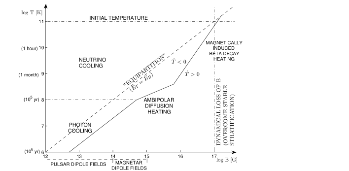
Figure 1: Magnetic field – temperature plane for a non-superfluid neutron star core. The dot-dashed horizontal lines show the initial temperature (just after core collapse), and the transition from neutrino-dominated (modified Urca) to photon-dominated cooling. The dashed diagonal line corresponds to the equality of magnetic and thermal energy. Above and to the left of the solid line, the star cools passively, on the time scales indicated in parenthesis along the vertical axis, without substantial magnetic field decay, so the evolution of the star is essentially a downward vertical line. Once the solid line is reached, magnetic dissipation mechanisms become important and generate heat that stops the cooling. The subsequent evolution is expected to be roughly along this line, with temperature and magnetic field decreasing together, much more slowly than the passive cooling.

On the other hand, in the strongly “suprathermal” regime, $|\eta|\mathrel{\hbox to0.0pt{\lower 4.0pt\hbox{$\sim$}\hss}\raise 1.0pt\hbox{$>$}}5kT$, the induced inverse beta decays leave more thermal energy in the star than is emitted in the form of neutrinos, i. e. in the region in which this chemical imbalance is present, the Urca processes have a net heating effect (Fernández & Reisenegger, 2005) and might therefore be able to keep the star warm during a time long enough for the field to decay (Thompson & Duncan, 1996). This heating-cooling balance occurs at

$$T_{8}\sim 2\leavevmode\nobreak\ B_{16}^{2}.$$ (37)

On this line (see Fig. 1), the thermal energy in the star,

$$E_{T}\sim 10^{46}\leavevmode\nobreak\ T_{8}^{2}\leavevmode\nobreak\ \mathrm{erg},$$ (38)

is less than its magnetic energy,

$$E_{B}\sim 10^{50}\leavevmode\nobreak\ B_{16}^{2}\leavevmode\nobreak\ \mathrm{erg},$$ (39)

by a factor

$$E_{T}/E_{B}\sim 2\times 10^{-4}\leavevmode\nobreak\ T_{8},$$ (40)

and therefore the cooling process of the star will be delayed by the inverse of this factor.

3.3.2 Ambipolar diffusion

At somewhat lower temperatures, collision rates are reduced (due to the increased degeneracy and reduced number of available quantum states), allowing different particle species to drift with respect to each other. The Lorentz force only acts directly on the charged particles (protons, electrons, and perhaps others), pushing them through the neutrons. The magnetic flux is only frozen into the charged particle fluid, which moves through the neutral fluid as fast as the balance of Lorentz force and collisions allows. If the charged fluid contains only protons and electrons, it will be barotropic. If additional particle species are present, it will be stably stratified due to their density-dependent abundances.

Goldreich & Reisenegger (1992) decompose the charged particle flux $n_{c}\@vec{v}_{c}$ of ambipolar diffusion into two modes:

• Irrotational, with $\nabla\cdot(n_{c}\@vec{v}_{c})\neq 0$ and $\nabla\times(n_{c}\@vec{v}_{c})=0$, which builds up pressure gradients in the charged particle fluid, which need to be eliminated by weak interactions in order for the motion to proceed.

• Solenoidal, with $\nabla\cdot(n_{c}\@vec{v}_{c})=0$ and $\nabla\times(n_{c}\@vec{v}_{c})\neq 0$, corresponding to an incompressible charged-particle flow, which does not cause pressure gradients and only needs to overcome the frictional force due to charged-neutron collisions.

The solenoidal mode is analogous to the motion of a barotropic, incompressible fluid, which should be enough to overcome the constraints imposed by stable stratification. In a non-superfluid $npe$ fluid, this mode proceeds on a time scale (Goldreich & Reisenegger, 1992)

$$t_{\mathrm{ambip}}^{\mathrm{s}}\sim 3\times 10^{3}{T_{8}^{2}\ell_{5}^{2}\over B_{15}^{2}}\leavevmode\nobreak\ \mathrm{yr},$$ (41)

causing a magnetic energy dissipation

$$-\dot{E}_{B}\sim 0.5\times 10^{44}\leavevmode\nobreak\ {B_{15}^{4}R_{6}^{3}\over\ell_{5}^{2}T_{8}^{2}}\leavevmode\nobreak\ \mathrm{erg\leavevmode\nobreak\ s^{-1}},$$ (42)

that can, at sufficiently low temperatures, balance the dominant cooling luminosity, be it neutrinos (here for the modified Urca process),

$$L_{\nu}\sim 3\times 10^{32}T_{8}^{8}\leavevmode\nobreak\ \mathrm{erg\leavevmode\nobreak\ s^{-1}},$$ (43)

or thermal electromagnetic radiation from the stellar surface,

$$L_{\gamma}\sim 10^{33}\leavevmode\nobreak\ T_{8}^{2.2}\leavevmode\nobreak\ \mathrm{erg\leavevmode\nobreak\ s^{-1}}.$$ (44)

The first will happen at $T_{8}\sim B_{15}^{2/5}$, and the second at $T_{8}\sim B_{15}^{0.95}$ (see Fig. 1).

3.3.3 Neutron star summary

Strongly magnetized neutron stars appear to be subject to processes that can erode the stable stratification and therefore cause an MHD-stable field to decay on time scales shorter than their observable lifetime. These processes are weak decays, which are dominant at very high field strengths, and ambipolar diffusion, at somewhat lower field strengths. In both cases, these processes become important only once the thermal energy in the star is substantially less than the magnetic energy, and therefore the latter acts as a large reservoir that keeps the star hot for much more than its cooling time in the un-magnetized case (see also Thompson & Duncan 1996; Pons et al. 2007). If the field decayed homologously, the star would evolve following the line of heating-cooling balance in Fig. 1. In fact, the evolution is likely more complex, involving loss of stability, followed by abrupt re-arrangements of the field (Braithwaite & Spruit, 2004), but these effects should occur roughly on the heating-cooling balance line.

Of course, neutron stars also have a solid crust, whose elastic and yielding properties are still highly uncertain. At very high field strengths, the Lorentz forces will distort the crust, which might act essentially as a fluid. At lower field strengths, the crust might act as a valve, controlling the loss of magnetic flux. The relative importance of the decay mechanisms in the crust (Hall drift, crust cracking) and core is still unclear, depending on the uncertain properties of both.

4 Conclusions

This paper contains a general discussion of several physical issues related to the existence of large-scale, coherent magnetic structures in upper main sequence stars, white dwarfs, and neutron stars. The main conclusions are the following:

• Magnetic forces in these objects are generally weak compared to pressure and gravity forces, and their matter is strongly stratified by entropy or composition gradients. This means that at least some components of the magnetic forces can easily be balanced by other forces. Thus, there can be a wide variety of possible equilibria. These equilibria are not force-free; in fact, force-free equilibria are not possible in stars.

• If the magnetic structure is axially symmetric, the only constraint it has to satisfy to be balanced by pressure and gravity forces is that the azimuthal component of the Lorentz force must vanish. This means that there must be a set of magnetic surfaces of toroidal topology containing both the magnetic field lines and the current flow lines. Since the fluid is not barotropic, there is no need for the magnetic field to satisfy a Grad-Shafranov equation.

• It is difficult to give general criteria for stability. However, it is likely that, in a stably stratified star, poloidal and toroidal field components of similar strength could stabilize each other. In a barotropic fluid, it is possible that no stable equilibria exist, as the magnetic field might rise buoyantly and be lost from the star.

• The long-term evolution of the magnetic field is likely to be governed by dissipative processes that erode the stable stratification. Heat diffusion in main sequence stars and white dwarfs appears to be too slow to cause an observable effect over the life time of these stars. In strongly magnetized neutron stars, ambipolar diffusion and beta decays might be causing the magnetic energy release observed in magnetars.

Appendix A No force-free fields in stars

Consider the following integral over a volume containing the star of interest:

$$\int_{\mathcal{V}}\mathbf{r}\cdot(\mathbf{j}\times\mathbf{B}/c)\leavevmode\nobreak\ d\mathcal{V}=\oint_{\mathcal{S}(\mathcal{V})}r_{i}T_{ij}ds_{j}-\int_{\mathcal{V}}T_{ii}d\mathcal{V}$$ (45)

(e. g. Kulsrud 2005, Chapter 4), where the Einstein summation convention is being used, and the magnetic stress tensor is

$$T_{ij}={B_{i}B_{j}\over 4\pi}-{B^{2}\over 8\pi}\delta_{ij}.$$ (46)

The last term in eq. (45) is minus the total magnetic energy within $\mathcal{V}$, $U_{B}=\int_{\mathcal{V}}B^{2}/(8\pi)\leavevmode\nobreak\ d\mathcal{V}>0$. The surface integral, taking the surface to be a sphere of radius $r$, becomes

$${1\over 8\pi}\oint d\Omega\leavevmode\nobreak\ r^{3}B^{2}\cos(2\beta),$$ (47)

where $\beta$ is the local angle between $\mathbf{B}$ and ${\mathbf{\hat{r}}}$. Outside a star, $B$ falls at least as fast as $r^{-3}$, so this integral goes to zero as $r\to\infty$. Thus, the only way to have $\mathbf{j}\times\mathbf{B}=0$ everywhere is to have $U_{B}=0$, i. e. $\mathbf{B}=0$ everywhere (except, perhaps, at a set of points of measure zero). This means that no magnetic stars can exist whose field is force-free everywhere. The “force-free” configurations of Pérez-Azorín et al. (2006) or Broderick & Narayan (2008) do not violate this theorem, because they have current sheets with infinite Lorentz forces on the stellar surface.

Appendix B Thermodynamic properties of a degenerate npe fluid

Taking the neutrons and protons to be nonrelativistic, the electrons extremely relativistic, and all highly degenerate, the total energy density and pressure are

$$\rho = nmc^{2}+{3\over 5}(n_{n}\tilde{\mu}_{n}+n_{p}\tilde{\mu}_{p})+{3\over 4}n_{e}\mu_{e},$$

$$P = n^{2}\left(\partial(\rho/n)\over n\right)_{Y}={2\over 5}(n_{n}\tilde{\mu}_{n}+n_{p}\tilde{\mu}_{p})+{1\over 4}n_{e}\mu_{e},$$ (48)

where $n_{n}=(1-Y)n$, $n_{p}=n_{e}=Yn$, $\mu_{e}=\hbar c(3\pi^{2}n_{e})^{1/3}$, $\tilde{\mu}_{i}=\mu_{i}-mc^{2}=\hbar^{2}(3\pi^{2}n_{i})^{2/3}$ for $i=n,p$. The chemical equilibrium state minimizes the energy per baryon with respect to $Y$ at fixed $n$, so in equilibrium $(\partial\rho/\partial Y)_{n}=0$. Thus, also evaluated at chemical equilibrium,

$$\left(\partial P\over\partial Y\right)_{\rho} = \left(\partial P\over\partial Y\right)_{n}=n\left[{2\over 3}(-\mu_{n}+\mu_{p})+{1\over 3}\mu_{e}\right]$$ (49)

$$= -{n\mu_{e}\over 3}.$$

The chemical imbalance $\eta=\mu_{n}-\mu_{p}-\mu_{e}=\tilde{\mu}_{n}-\tilde{\mu}_{p}-\mu_{e}=-(1/n)(\partial\rho/\partial Y)_{n}$ satisfies

$$\left(\partial\eta\over\partial Y\right)_{\rho} = \left(\partial\eta\over\partial Y\right)_{n}=-{2\over 3}{\tilde{\mu}_{n}\over 1-Y}-{2\over 3}{\tilde{\mu}_{p}\over Y}-{1\over 3}{\mu_{e}\over Y}$$ (50)

$$\approx -{\mu_{e}\over 3Y}.$$

So,

$$\left(\partial P\over\partial\eta\right)_{\rho}\approx nY=n_{e}=n_{p}.$$ (51)