Probing spatial spin correlations of ultracold gases by quantum noise spectroscopy

Abstract

Spin noise spectroscopy with a single laser beam is demonstrated theoretically to provide a direct probe of the spatial correlations of cold fermionic gases. We show how the generic many-body phenomena of anti-bunching, pairing, antiferromagnetic, and algebraic spin liquid correlations can be revealed by measuring the spin noise as a function of laser width, temperature, and frequency.

Ultracold atoms offer the possibility to prepare, manipulate and probe various paradigm phases of strongly correlated systems. Considerable efforts are devoted to develop sensitive detection schemes to study these phases. Whereas most experiments in this field are based on measuring mean values of various observables, further insight can be obtained from the correlations in the noise of the atomic distribution Altman ; folling ; Hofferberth . In recent experiments a new technique using phase contrast imaging was used to probe the spin of ultracold atoms sadler06 ; shin06 . In related experiments shp ; sherson ; windpassinger similar techniques have been pushed to the point where they are sensitive to the quantum fluctuations of the atoms. In this Letter, we show that quantum spin noise spectroscopy along the lines of Refs. sadler06 ; shin06 ; shp ; sherson ; windpassinger constitutes a sensitive probe of the correlations of the underlying quantum state. We focus on generic many-body phenomena such as antibunching, pairing, and spin liquids. Furthermore, we show that spin noise measurement is an ideal tool for probing antiferromagnetic ordering and phase transitions for atoms in optical lattices, which is currently one of the main challenges in cold atoms physics. Related theoretical studies of spin noise have recently been presented in Refs. Eckert ; mihaila ; Cherng .

Quantum noise limited probing of the spin state may be obtained either by polarization rotation shp ; sherson or phase contrast imaging oblak ; windpassinger . In the first approach the spin imprints a phase shift on a laser beam and this phase shift is subsequently measured by interfering the beam with another laser beam (i.e. homodyne detection). In the polarization rotation measurement the two laser beams are replaced by two different polarization modes, which has the advantage that the setup is less sensitive to fluctuations in optical path length and beam profile. Ideally one would probe the system by imaging with a camera, but here we explore a slightly simpler situation where a laser beam is passed through the sample and the final result is measured by photo detectors without any spatial resolution. In the limit of strong beams (many photons) experiencing a small phase change, the observable, i.e. the measured light quadrature in the homodyne detection, may be expressed as sherson ; oblak ; sorensen ; Carusotto

$$\hat{X}_{{\rm out}}=\hat{X}_{{\rm in}}+\frac{\kappa}{\sqrt{2}}\hat{M}_{z}.$$ (1)

Here, $\hat{X}_{{\rm in/out}}$ is a canonical position operator describing the light normalized such that the input corresponds to vacuum noise $\langle\hat{X}_{{\rm in}}^{2}\rangle=1/2$, and $\kappa$ is a coupling constant. The effective measured atomic operator is $\hat{M}_{z}=\int d^{3}r\ \phi({\mathbf{r}})\hat{s}_{z}({\mathbf{r}})/\sqrt{A},$ where $A=\int d^{3}r\phi^{2}({\mathbf{r}})n({\mathbf{r}})/4$ is a normalization constant, $\phi({\mathbf{r}})$ is the spatial intensity profile of the laser beam, and $\hat{s}_{z}({\mathbf{r}})=(\hat{\psi}^{\dagger}_{\uparrow}({\mathbf{r}})\hat{\psi}_{\uparrow}({\mathbf{r}})-\hat{\psi}^{\dagger}_{\downarrow}({\mathbf{r}})\hat{\psi}_{\downarrow}({\mathbf{r}}))/2=(\hat{n}_{\uparrow}({\mathbf{r}})-\hat{n}_{\downarrow}({\mathbf{r}}))/2$ gives the local population imbalance (magnetization) with $\hat{\psi}_{\sigma}({\mathbf{r}})$ being the atomic field operator. We consider a two-component atomic gas ($\sigma=\uparrow,\downarrow$) with total local density $n({\mathbf{r}})=\langle\hat{n}_{\uparrow}({\mathbf{r}})+\hat{n}_{\downarrow}({\mathbf{r}})\rangle$ and assume Gaussian laser profiles $\phi({\mathbf{r}})\propto e^{-(x^{2}+y^{2})/d^{2}}.$ By measuring the observable $\hat{X}_{{\rm out}}$ it is possible to obtain spatially resolved information about the magnetization $\langle\hat{X}_{{\rm out}}\rangle=\kappa\langle\hat{M}_{z}\rangle/\sqrt{2}$. In many cases, however, interesting states may not have any net magnetization $\langle\hat{M}_{z}\rangle=0$. In this Letter, we will only consider such situations and show that a measurement of the quantum noise $\langle\hat{X}_{{\rm out}}^{2}\rangle=(1+R\kappa^{2})/2$, where $R\equiv\langle\hat{M}_{z}^{2}\rangle$ giving

$$R=\frac{1}{A}\int d^{3}r_{1}d^{3}r_{2}\phi({\mathbf{r}}_{1})\phi({\mathbf{r}}_{2})\langle\hat{s}_{z}({\mathbf{r}}_{1})\hat{s}_{z}({\mathbf{r}}_{2})\rangle$$ (2)

provides insight into the state of the system. Since $R$ is quadratic in the atomic density operators it gives a direct measure of the atomic correlations in the system. The normalization in Eq. (2) is chosen such that the quantum noise of an uncorrelated state, where each atom has an equal probability of being in each of the two internal states, is $R=1$ (standard quantum limit).

We first consider the normal phase, where the spin fluctuations have a length scale of $k_{F}^{-1}$. It follows that $R$ vanishes if the effective volume $V_{B}=(\int_{V}d^{3}r\phi)^{2}/\int_{V}d^{3}r\phi^{2}$ is large, $V_{B}\gg k_{F}^{-3}$. Fermi statistics thus suppresses the noise below the standard quantum limit $R=1$. For a finite laser beam there will, however, be a noise contribution from the boundary $\langle M_{z}^{2}\rangle\sim d$, which translate into $R\sim 1/k_{F}d$.

A key property of pairing for fermions is that the two particle density matrix $\langle\psi_{\uparrow}^{\dagger}(\mathbf{r}_{1})\psi_{\downarrow}^{\dagger}(\mathbf{r}_{2})\psi_{\downarrow}(\mathbf{r^{\prime}}_{2})\psi_{\uparrow}(\mathbf{r^{\prime}}_{1})\rangle$ has a macroscopic eigenvalue $p_{c}N$ with $N$ the number of particles and $p_{c}$ the condensate fraction. Spin noise spectroscopy probes the two particle density matrix directly, and in the large $d$ limit the noise is dominated by the largest eigenvalue $p_{c}N$. The noise depends on the shape of the applied laser beam as seen from the following argument: assuming a top hat laser profile with a radius $d$ and sharp edges compared to the radius $\xi$ (coherence length) of the pair wavefunction $\chi(\mathbf{r})$, the noise is proportional to the number of pairs within $\xi$ of the edge such that only one particle is inside the beam. This gives a scaling $R\propto 1/d$ as in the normal case. With a smooth laser profile with radius $d$ and fall-off distance $D>\xi$, the noise is due to pairs in the edge region. These pairs couple to the gradient ($\sim 1/D$) and the noise from the difference in signal from $\uparrow$ and $\downarrow$ particles is $\sim\int d^{3}r\chi^{2}(r)r^{2}/D^{2}\sim\xi^{2}/D^{2}$. This should be multiplied by the number of pairs in the edge region $\sim L_{z}dDp_{c}N/V$, where $L_{z}$ and $V$ denote the length and volume of the system. Since $A\sim L_{z}d^{2}N/V$, we get $R\sim p_{c}\xi^{2}/Dd$. With a Gaussian beam $D\sim d$, and the scaling $R\sim p_{c}\xi^{2}/d^{2}$ thus provides a measurement of $\xi$ and $p_{c}$.

We now use the BCS wavefunction to derive this scaling rigorously in the BCS and BEC limits. Consider a homogeneous gas with constant density $n_{\sigma}({\mathbf{r}})=N_{\sigma}/V$. Wicks theorem yields $\langle\hat{s}_{z}({\mathbf{r}}_{1})\hat{s}_{z}({\mathbf{r}}_{2})\rangle=n\delta({\mathbf{r}})-2\theta^{2}(r)-2F^{2}(r)$ with ${\mathbf{r}}={\mathbf{r}}_{1}-{\mathbf{r}}_{2}$, $\theta(r)=\langle\hat{\psi}^{\dagger}_{\sigma}({\mathbf{r}}_{1})\hat{\psi}_{\sigma}({\mathbf{r}}_{2})\rangle$, and $F(r)=\langle\hat{\psi}_{\uparrow}({\mathbf{r}}_{1})\hat{\psi}_{\downarrow}({\mathbf{r}}_{2})\rangle$. We then find

$$R=1-\frac{2}{A}\int d^{3}r_{1}d^{3}r_{2}\phi({\mathbf{r}}_{1})\phi({\mathbf{r}}_{2})[\theta^{2}(r)+F^{2}(r)].$$ (3)

In the BEC regime $k_{F}a\rightarrow 0_{+}$, the chemical potential is $\mu\rightarrow-\hbar^{2}/2ma^{2}$. This gives $u_{k}v_{k}\rightarrow\Delta/2(|\mu|+k^{2}/2m)$ and $v_{k}^{2}\rightarrow\Delta^{2}/4(|\mu|+k^{2}/2m)^{2}$ for the coherence factors defined as $u^{2}=(1+\xi/E)/2$, $v^{2}=1-u^{2}$ with $E=(\xi^{2}+\Delta^{2})^{1/2}$ and $\xi=k^{2}/2m-\mu$. We obtain $\theta(r)/n_{\sigma}=\exp(-r/a)$ and $F(r)/n_{\sigma}=\sqrt{3\pi/k_{F}a}\exp(-r/a)/k_{F}r$ which is proportional to the asymptotic bound state wavefunction for a potential with scattering length $a$. Likewise, in the BCS limit $k_{F}a\rightarrow 0_{-}$, $\theta(r)/n_{\sigma}=3[\sin k_{F}r-k_{F}r\cos k_{F}r\sqrt{\pi r/2\xi}\exp(-r/\xi)]/(k_{F}r)^{3}$ and $F(r)/n_{\sigma}=3\sin k_{F}r\sqrt{\pi/2\xi r}\exp(-r/\xi)/k_{F}^{2}r$ for $r\rightarrow\infty$ where $\xi=k_{F}/m\Delta$ ($\hbar=1$) and $\Delta$ is the gap. Using these limiting forms in (3), we obtain for $d\rightarrow\infty$

$$\begin{array}[]{c || c | c | c}&\rm{Normal\>phase}&\rm{BCS\>limit}&\rm{BEC\>limit}\\ \hline\cr R(d)&\frac{3\pi^{1/2}}{2^{5/2}}\frac{1}{k_{F}d}&\frac{\xi}{4k_{F}d^{2}}&\frac{a^{2}}{6d^{2}}\end{array}.$$ (4)

For $s$-wave interactions, the pair wavefunction has a short-range divergence (bunching) given by $F(r)=m\Delta/4\pi r$ Bruun resulting in a linear decrease of the noise for $k_{F}d\rightarrow 0$ in both the BCS and BEC limits. Using $p_{c}\sim 1/k_{F}\xi$, the BCS result agrees with the estimate given in the previous section.

In Fig. 1, we plot $R(d)$ for a homogeneous system of transverse radius $L=100k_{F}^{-1}$ at $T=0$. Results for the normal phase and the superfluid phase with $(k_{F}a)^{-1}=-1$ (BCS regime), $(k_{F}a)^{-1}=0$ (unitary limit), and $(k_{F}a)^{-1}=2$ (BEC regime) are shown. The noise is calculated numerically from (3) using the BCS wavefunction.

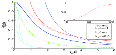
Figure 1: (Color online) Noise $R(d)$ for various coupling strengths. The thin lines show the $d\rightarrow\infty$ limit (4). The inset shows the large $d$ behavior $d/L\sim{\mathcal{O}}(1)$ with $\beta=1$ for the normal phase and the superfluid phase in the BEC limit.

The noise is below the quantum limit $R\leq 1$ and $R\rightarrow 0$ for $d\rightarrow\infty$ in agreement with the analysis above. Pairing suppresses the noise compared to the normal state due to positive correlations between opposite spin states. The suppression increases with the pairing moving toward the BEC side.

For very large $d$ the laser probes a significant fraction of the system and it is important to include possible spin fluctuations due to the experimental preparation of the system. Typically, such fluctuations will at least be limited by the standard quantum limit, i.e. $R=\beta$ with $\beta\gtrsim 1$ when probing the entire system. When probing a sub-system this gives an extra contribution $\sim\beta V_{B}/V$ which is important for large $d$ for the normal phase and the superfluid phase on the BEC side $(k_{F}a)^{-1}=2$ (see inset in Fig. 1). However, this term is absent for $(k_{F}a)^{-1}\lesssim 0.5$, since superfluidity quenches the spin noise in this regime Shin ; Pilati ; NoiseEdge . Observing $R\ll 1$ for a large portion of the sample would represent an extreme experimental demonstration of this quenching.

The observed enhancement of the nuclear spin relaxation just below the transition temperature $T_{c}$ (Hebel-Slichter effect) constitutes one of the hallmark experimental tests of BCS theory. We now demonstrate the existence of a spin noise spectroscopy analogy to the Hebel-Slichter effect. Similar effects has been demonstrated to occur in inelastic light scattering and Bragg scattering experiments BruunSlichter . The probing technique discussed in this Letter is in principle non-destructive. By recoding the signal for a long duration of time one can thus obtain all frequency components of the noise $R(d,\omega)$ by Fourier analysis mihaila , i.e. Fourier transforming the measured $\hat{X}_{{\rm out}}(t)$ provides a measurement of $M_{z}(\omega)$. Such probing will have similar signal-to-noise ratio $\kappa^{2}(\omega)\sim\eta\alpha$, but since spontaneous emission may lead to significant heating $\eta$ may have to be kept very low to avoid that the system heats up during the measurement. Using (3) we obtain for a homogeneous system

$$R(d,\omega)=\frac{8\pi md^{2}}{n}\int\frac{d^{3}k}{(2\pi)^{3}}\frac{E^{\prime}}{\sqrt{E^{\prime 2}-\Delta^{2}}}(uu^{\prime}+vv^{\prime})^{2}$$

$$\times f(1-f^{\prime})e^{-({\mathbf{k}}_{\perp}-{\mathbf{k}}_{\perp}^{\prime})^{2}d^{2}/2}I_{0}(k_{\perp}k^{\prime}_{\perp}d^{2})$$ (5)

where $I_{0}$ is the modified Bessel function of the first kind, ${\mathbf{k}}_{\perp}=(k_{x},k_{y})$ is the transverse momentum, and $f=[\exp(\beta E)+1]^{-1}$. The primed quantities refer to the momentum $\mathbf{k}^{\prime}$ with energy $E^{\prime}=E+\omega$. There is momentum conservation along the $z$-direction with $k_{z}^{\prime}=k_{z}$ whereas ${\mathbf{k}}^{\prime}_{\perp}\neq{\mathbf{k}}_{\perp}$ due to the transverse Gaussian profile. Eq. (5) gives the noise contribution from quasiparticle scattering from momentum ${\mathbf{k}}$ to ${\mathbf{k}}^{\prime}$. There are additional terms describing pair breaking and quasiparticle absorption which do not affect the Hebel-Slichter effect.

In Fig. 2, we plot $R(d,\omega)$ as a

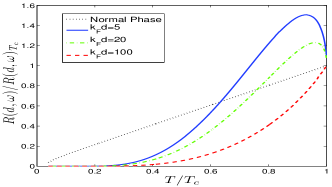
Figure 2: (Color online) $R(d,\omega)$ in units of $R(d,\omega)$ at $T_{c}$ for various laser widths $d$ and $k_{F}a=-1$.

function of $T/T_{c}$ calculated numerically from (5) using the self-consistently determined gap $\Delta(T)$. We have chosen $k_{F}a=-1$ giving $T_{c}/T_{F}\simeq 0.13$ and $\omega/k_{B}T_{c}=0.08$ since the Hebel-Slichter effect only occurs for $\omega\lesssim k_{B}T_{c}$. For narrow laser widths, a Hebel-Slichter peak is prominent below $T_{c}$. The peak arises from an increased density of states at the gap edge; it decreases with increasing $d$ and disappears for $d\gg\xi(T=0)\simeq 9$. This is because for large laser widths, the scattering becomes subject to momentum conservation which restricts the available phase space.

Quantum systems in periodic potentials constitute another class of intriguing systems which can be examined by cold atomic gases using optical lattices. Superfluidity in lattices, possibly of $d$-wave symmetry, can be detected by suppression of spin noise similar to the discussion above for homogeneous systems. The only difference is that the $d$-wave pair wavefunction does not diverge for short length scales and there is no linear decrease in $R$ for small laser radii $d$. One could use a laser with elliptical transverse profile to detect the anisotropic suppression of spin noise due to the $d$-wave symmetry of the pairing.

Presently, a main experimental goal in optical lattices is to observe the onset of antiferromagnetic (AF) correlations with decreasing temperature Jordens . As demonstrated below, spin noise spectroscopy can measure the magnetic susceptibility of the system and hence constitutes an important experimental probe of the spin correlations. As an example, we study atoms described by the Hubbard model which in the strong repulsion limit at half filling for $kT\ll U$ reduces to the AF Heisenberg model, $H=J\sum_{\langle i,j\rangle}\textbf{s}_{i}\cdot\textbf{s}_{j}$, where $\langle i,j\rangle$ denotes nearest neighbor pairs and $\textbf{s}_{i}$ is the spin $1/2$ operator for the atoms at site $i$. Assuming, without loss of generality, a staggered magnetization along the $z$-direction, we now show how to detect AF correlations by measuring $R_{\parallel}\equiv\langle\hat{M}_{z}^{2}\rangle$ and $R_{\perp}\equiv\langle\hat{M}_{x}^{2}\rangle$, where $M_{x}$ is defined analogous to $M_{z}$. (A preferred direction for the broken symmetry can be induced by enforcing a slight anisotropy in the exchange coupling $J$.) Here we are mainly interested in the $T$ dependence and focus on the situation where we probe the entire ensemble. Therefore, we assume a broad laser profile with $\phi=1$ in (2) such that $R_{\parallel(\perp)}=4\langle S_{z(x)}S_{z(x)}\rangle/N$ with ${\mathbf{S}}=\sum_{i}{\mathbf{s}}_{i}$ and $N$ is the number of spins. In the paramagnetic phase, $R_{\parallel}=R_{\perp}=4kT\chi$ where $\chi$ is the magnetic susceptibility. A high temperature expansion yields for the 2D square and 3D cubic lattices DombGreen

$$4kT\chi=\left\{\begin{array}[]{lcl}1-2x+2x^{2}-1.333x^{3}+\ldots&,&\rm{2D}\\ 1-3x+6x^{2}-11x^{3}+\ldots&,&\rm{3D}\end{array}\right.$$ (6)

where $x=J/2kT$. In 2D, the system remains paramagnetic for $T>0$, and modified spin-wave theory yields $\chi=(12J)^{-1}[0.524+0.475T/J+{\mathcal{O}}(T^{3})]$ for $T/J\ll 1$ Takahashi . In the 3D case, the system undergoes a phase transition to an AF phase at the Néel temperature $T_{N}$. In the AF phase, $R_{\parallel}\neq R_{\perp}$. Using spin-wave theory for $T<T_{N}$, we obtain $R_{\perp}=kT/(3J)$ and

$$R_{\parallel}=\frac{4}{N}\sum_{\mathbf{k}}\frac{1}{2\sinh^{2}(\beta\omega_{\mathbf{k}}/2)}.$$ (7)

Here $\omega_{\mathbf{k}}=3J\sqrt{1-\gamma_{\mathbf{k}}^{2}}$ is the spin-wave energy with $\gamma_{\mathbf{k}}=(\cos k_{x}a+\cos k_{y}a+\cos k_{z}a)/3$ for a cubic lattice with lattice constant $a$. The sum in (7) is over the reduced Brillouin zone. For $kT\ll J$, (7) yields $R_{\parallel}=4(kT)^{3}/(3s^{3})$, with $s=\sqrt{3}J$ the spin-wave velocity. In Fig.  3 we plot these results for both the 2D and 3D systems.

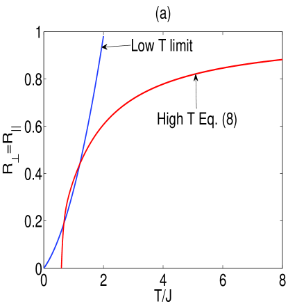
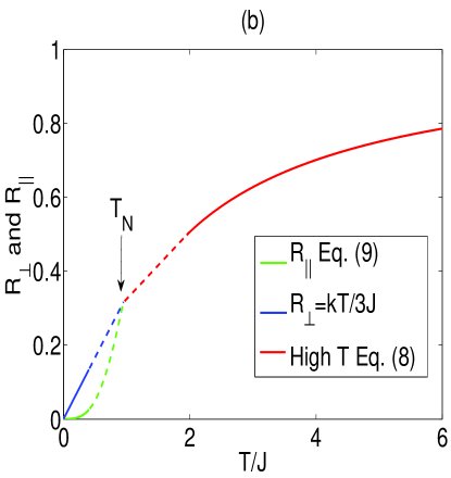
Figure 3: (Color online) $R_{\parallel}$ and $R_{\perp}$ for a 2D (a) and 3D (b) system. Solid lines are the high and low $T$ results discussed in the text and the dashed lines in (b) (obtained by simple rescaling) indicate how they meet at $T_{N}\simeq 0.946J$ Sandvik .

We see that the onset of AF correlations in the paramagnetic phase can be detected as a decrease in the noise from the uncorrelated result $R_{\parallel}=R_{\perp}=1$ as described by (6). By comparing with the high temperature expansion, the spin noise may even serve as an accurate thermometer for the spin temperature. Furthermore, the AF phase for the 3D case can be detected by observing $R_{\parallel}\neq R_{\perp}$. An advantage of probing collective operators like $S_{z}$ is that they are conserved, and therefore could be measured after time of flight. In this case, however, special care has to be taken of the contribution from the boundary region. We do not expect the trapping potential to change these results qualitatively Andersen ; snoek .

The method presented here can also be used to probe the correlations of more exotic quantum phases such as resonating valence bond states and algebraic spin liquids hermele . These states are characterized by long-range spin correlations $\langle{\mathbf{s}}({\mathbf{r}}){\mathbf{s}}(0)\rangle\sim(-1)^{r_{x}+r_{y}}/r^{(1+\eta)}$. Techniques exist for addressing, e.g., every second site in a lattice peil . Flipping every second spin before the measurement ($s_{z}\rightarrow(-1)^{r_{x}+r_{y}}$) will give $\langle s_{z}({\mathbf{r}})s_{z}(0)\rangle\sim 1/r^{(1+\eta)}$. Performing noise spectroscopy on this state will give a contribution from the long-range correlations $R\sim d^{(1-\eta)}$. By measuring the scaling of $R$ with $d$ one can thus directly determine the exponent $\eta$ of the spin correlations.

Finally we consider the experimental requirements for realizing our scheme. The experiments should be quantum noise limited with all classical noise sources suppressed. This has already been achieved in several experiments shp ; sherson ; windpassinger ; oblak , and we expect it to be simpler to realize for the smaller systems considered here. In addition, the atomic noise should be large compared to the light noise inherently present in the probe. The spontaneous emission probability pr. atom caused by the probing light is $\eta\sim\kappa^{2}/\alpha$, where $\alpha=3nL_{z}\lambda^{2}\gamma_{x}/\gamma 2\pi$ is the optical depth of the ensemble sherson ; oblak ; sorensen . Taking $n\sim 10^{12}$ cm^-3, $L_{z}\sim 100$ $\mu$m, a probing wavelength $\lambda=671$ nm corresponding to Li, and a branching ratio $\gamma_{x}/\gamma=1/2$ gives $\alpha=16$ for a harmonically trapped Fermi gas. For atoms in optical lattices at half filling $\alpha\approx N_{s}=50$ where $N_{s}$ is the number of lattice sites in each direction. One can thus have a large signal-to-noise ratio $\kappa^{2}R\gtrsim 1$ with very little noise added from spontaneous emission during the probing $\eta=\kappa^{2}/\alpha\ll 1$. Another concern is the spatial resolution. Experimentally, one may obtain a resolution down to $d\sim 5\lambda$ shin06 . Taking $n\sim 10^{12}$cm^-3 this corresponds to $k_{F}d\sim 10$. Thus, it may require an adiabatic expansion of the gas to observe the small scale limit of Fig. 1. However, it is possible directly to observe the large $d$ scaling, the Hebel-Slichter effect, and the onset of magnetic correlations.

In summary, we have shown how to extract the correlations of quantum states of ultracold atoms using spin noise spectroscopy. This was demonstrated explicitly by calculating the spin noise for normal Fermi gasses, superfluids, paramagnetic and AF phases and algebraic spin liquids. This method can be applied to other strongly correlated systems as well as extended to higher order moments Cherng . It may even be extended to full quantum state tomography of the two particle density matrix.

We acknowledge useful conversations with R. Cherng, E. Polzik, A. Sanpera. Partial support was provided by the Villum Kann Rasmussen Foundation (B. M. A.) and the Harvard-MIT CUA, DARPA, MURI, and the NSF grant DMR-0705472 (E. D.).

References

- (1) E. Altman, E. Demler, and M. Lukin, Phys. Rev. A 70, 013603 (2004).
- (2) S. Fölling et al. Nature 434, 481 (2005); M. Greiner et al., Phys. Rev. Lett. 94, 110401 (2005).
- (3) S. Hofferberth et al. Nat. Phys. 4, 489 (2008); I. B. Spielman, W. D. Phillips, and J. V. Porto, Phys. Rev. Lett. 98, 080404 (2007); V. Guarrera et al., ibid. 100, 250403 (2008); Z. Hadzibabic et al., ibid. 93, 180403 (2004).
- (4) Y. Shin et al., Phys. Rev. Lett. 97, 030401 (2006).
- (5) L. E. Sadler et al., Nature 443, 312 (2006).
- (6) J. L. Sørensen, J. Hald, and E. S. Polzik, Phys. Rev. Lett. 80, 3487 (1998).
- (7) J. Sherson, B. Julsgaard, and E. S. Polzik, Adv. At. Mol. Opt. Phys. 54, 81 (2006).
- (8) P. J. Windpassinger et al., Phys. Rev. Lett. 100, 103601 (2008).
- (9) K. Eckert et al., Phys. Rev. Lett. 98, 100404 (2007); K. Eckert et al., Nature Phys. 4, 50 (2008).
- (10) B. Mihaila et al., Phys. Rev. A 74, 063608 (2006).
- (11) R. W. Cherng and E. Demler, New J. Phys. 9:7 (2007)
- (12) D. Oblak et al., Phys. Rev. A 71, 043807 (2005).
- (13) M. W. Sørensen and A. S. Sørensen Phys. Rev. A 77, 013826 (2008).
- (14) I. Carusotto, J. Phys. B: At. Mol. and Opt. Phys. 39, S211 (2006).
- (15) G. M. Bruun et al., Eur. Phys. J. D 7, 433 (1999).
- (16) Y. Shin et al., Nature 451, 689 (2008).
- (17) S. Pilati and S. Giorgini, Phys. Rev. Lett. 100, 030401 (2008).
- (18) We assume the laser does not probe the far edges of the gas where any spin imbalance exists as a normal phase.
- (19) G. M. Bruun and G. Baym, Phys. Rev. Lett. 93, 150403 (2004); Phys. Rev. A 74, 033623 (2006).
- (20) R. Jördens et al., arXiv:0804.4009v1.
- (21) G. S. Rushbrooke, G. A. Baker, Jr., and P. J. Wood, in Phase Transitions and Critical Phenomena, edited by C. Domb and M. S. Green (Academic), Vol. 3, Chap. 5.
- (22) M. Takahashi, Phys. Rev. B 40, 2494 (1989).
- (23) A. W. Sandvik, Phys. Rev. Lett. 80, 5196 (1998).
- (24) B. M. Andersen and G. M. Bruun, Phys. Rev. A 76, 041602 (2007).
- (25) M. Snoek et al., New J. Phys. 10, 093008 (2008).
- (26) M. Hermele, T. Senthil and M. P. A. Fisher, Phys. Rev. B 72, 104404 (2005)
- (27) S. Peil et al., Phys. Rev. A 67, 051603 (2003).