All-sky search of NAUTILUS data

Abstract

A search for periodic gravitational-wave signals from isolated neutron stars in the NAUTILUS detector data is presented. We have analyzed half a year of data over the frequency band $\langle 922.2;\,923.2\rangle$ Hz, the spindown range $\langle-1.463\times 10^{-8};\,0\rangle$ Hz/s and over the entire sky. We have divided the data into 2 day stretches and we have analyzed each stretch coherently using matched filtering. We have imposed a low threshold for the optimal detection statistic to obtain a set of candidates that are further examined for coincidences among various data stretches. For some candidates we have also investigated the change of the signal-to-noise ratio when we increase the observation time from two to four days. Our analysis has not revealed any gravitational-wave signals. Therefore we have imposed upper limits on the dimensionless gravitational-wave amplitude over the parameter space that we have searched. Depending on frequency, our upper limit ranges from $3.4\times 10^{-23}$ to $1.3\times 10^{-22}$. We have attempted a statistical verification of the hypotheses leading to our conclusions. We estimate that our upper limit is accurate to within $18$%.

1 Introduction

We present results of the search of the NAUTILUS (a resonant bar detector [1]) data for periodic gravitational-wave (GW) signals. We search the band $\langle 922.2;\,923.2\rangle$ Hz and the spindown range $\langle-1.463\times 10^{-8};\,0\rangle$ Hz/s over the entire sky. We analyze NAUTILUS data collected in the year 2001. We divide the data into stretches of 2 sidereal days. Each stretch of data is analyzed coherently using matched filtering in the form of the ${\mathcal{F}}$-statistic [2, 3]. We have analyzed slightly more than half a year of data.

Previous analysis of bar detector data for periodic GW signals were the search of the galactic center and the globular cluster 47 Tucanae with the ALEGRO detector [4], the search of the galactic center using the EXPLORER detector data [5], and an all-sky search using the EXPLORER data [6, 7]. LIGO (Laser Gravitational Wave Observatory) data was searched for known pulsars [8, 9, 10], over the entire sky [11] using the coherent method and over all the sky using incoherent methods [12, 13]. Currently LIGO data are analyzed over the entire sky by the Einstein@Home project [14].

In section 2 we present the data analysis methods used in our search. In section 3 we outline our search procedure. In section 4 we discuss the analysis of the candidates. This analysis consists of two parts: the first part is the search for coincidences between the candidates each obtained from a different stretch of data and the second part is an investigation of the increase of the signal-to-noise ratio of candidates when we increase the observation time from two to four days. In section 5 we impose upper limits on amplitudes of the gravitational waves in the parameter space that we have searched.

2 Data analysis methods

In order to search for gravitational waves from long lived periodic sources we have used the maximum likelihood (ML) method. For the case of Gaussian noise the ML method consists of linearly filtering the data with a template matched to the signal that we are searching for. The main complication of the matched filtering is that the signal depends on several unknown parameters. This requires evaluation of the likelihood function over a large parameter space. In order to minimize the computation time we use several data analysis tools. Firstly we find the maximum likelihood estimators of some parameters (4 in the case of a GW signal from a rotating neutron star that we are searching for) in a closed analytic form, thereby reducing the dimensionality of the parameter space that we have to search. The likelihood function over the reduced parameter space is called the ${\mathcal{F}}$-statistic and it is derived in [2]. Secondly we analyze data of length equal to an integer multiple of a sidereal day. This leads to a considerable simplification of the ${\mathcal{F}}$-statistic and consequently reduces the number of numerical operations to evaluate it. The ${\mathcal{F}}$-statistic for observation time equal to an integer number of sidereal days is given in section III of [15]. Thirdly we use optimal numerical algorithms, in particular the Fast Fourier Transform (FFT) in order to calculate the ${\mathcal{F}}$-statistic efficiently. Fourthly we minimize the number of ${\mathcal{F}}$-statistic calculations over the parameter space by solving a covering problem for this space [16, 17]. Let us explain the latter two data analysis tools in more detail. The response of a bar detector to a gravitational-wave signal from a spinning neutron star is summarized in section 2.1 of [7].

Fast Fourier Transform. Estimates have shown [21, 20] that for the bandwidth and the spindown range that we search we need to take into account in our templates only one spindown parameter in order to match the signal. Consequently the phase modulation function $\phi(t)$ of the waveform is given by

$$\phi(t)=\omega_{0}t+\omega_{1}t^{2}+(\omega_{0}+2\omega_{1}t)\frac{{\bf n}_{0}\cdot{\bf r}_{\rm d}(t)}{c},$$ (1)

where $\omega_{0}$ is angular frequency and $\omega_{1}$ is the spindown parameter, $\mathbf{n}_{0}$ is the constant unit vector in the direction of the star in the Solar System Barycenter (SSB) reference frame (it depends on the right ascension $\alpha$ and the declination $\delta$ of the source), and ${\bf r}_{\rm d}$ is the vector joining the SSB with the detector and $c$ is the speed of light. The detection statistic ${\mathcal{F}}$ involves two integrals of the form

$$F=\int^{T_{0}}_{0}x(t)\,a(t)\,e^{-i\phi(t)}\,\mathrm{d}t,$$ (2)

where $x(t)$ is the data stream, $a(t)$ is the amplitude modulation function that depends on $\delta$ and $\alpha$. The above integral is not a Fourier transform because the frequency $\omega_{0}$ in the phase multiplies the term ${\bf n}_{0}\cdot{\bf r}_{\rm d}(t)$ which is a non linear function of time. In order to convert the integral into a Fourier transform we introduce the following interpolation procedure. The phase $\phi(t)$ [Equation (1)] can be written as

$$\phi(t)=\omega_{0}[t+\phi_{\mathrm{m}}(t)]+\phi_{\mathrm{s}}(t),$$ (3)

where

$$\phi_{\mathrm{m}}(t) :=\frac{{\bf n}_{0}\cdot{\bf r}_{\rm d}(t)}{c},$$ (4)

$$\phi_{\mathrm{s}}(t) :=\omega_{1}t^{2}+2\frac{{\bf n}_{0}\cdot{\bf r}_{\rm d}(t)}{c}\omega_{1}t.$$ (5)

The functions $\phi_{\mathrm{m}}(t)$ and $\phi_{\mathrm{s}}(t)$ do not depend on the angular frequency $\omega_{0}$. We can write the integral (2) as

$$F=\int^{T_{0}}_{0}x(t)\,a(t)\,e^{-i\phi_{\mathrm{s}}(t)}\exp\big{\{}-i\omega_{0}[t+\phi_{\mathrm{m}}(t)]\big{\}}\,\mathrm{d}t.$$ (6)

We see that the integral (6) can be interpreted as a Fourier transform (and computed efficiently with an FFT), if $\phi_{\mathrm{m}}=0$. In order to convert equation (6) to a Fourier transform we introduce a new time variable $t_{b}$, so called barycentric time [18, 2],

$$t_{b}:=t+\phi_{\mathrm{m}}(t).$$ (7)

In the new time coordinate the integral (6) is approximately given by (see Ref. [2], Sec. IIID)

$$F\cong\int^{T_{0}}_{0}x[t(t_{b})]a[t(t_{b})]e^{-i\phi_{\mathrm{s}}[t(t_{b})]}e^{-i\omega_{0}t_{b}}\,\mathrm{d}t_{b}.$$ (8)

Thus in order to compute the integral (6), we first multiply the data $x(t)$ by the function $a(t)\,\exp[-i\phi_{\mathrm{s}}(t)]$ for each set of the parameters $\omega_{1},\delta,\alpha$ and then resample the resulting function according to equation (7). At the end we perform the FFT.

The covering problem. The covering problem is to find the minimum number of templates in the parameter space [17], so that the fractional loss in signal to ratio is not less than $1-MM$ ($MM$ is the minimal match parameter introduced by Owen [22]). In order to solve the covering problem we introduce a useful approximate model of the gravitational-wave signal from a rotating neutron star. The model relies on (i) neglecting all spindowns in the phase modulation due to motion of the detector with respect to the SSB; and (ii) discarding the component of the vector ${\bf r}_{\rm d}$ (connecting the SSB and the detector) which is perpendicular to the ecliptic plane. These approximations lead to the following phase model of the signal:

$$\phi_{\mathrm{lin}}(t)=\omega_{0}t+\omega_{1}t^{2}+\alpha_{1}\mu_{1}(t)+\alpha_{2}\mu_{2}(t),$$ (9)

where $\alpha_{1}$ and $\alpha_{2}$ are new constant parameters,

$$\alpha_{1} :=\omega_{0}(\sin\alpha\cos\delta\cos\varepsilon+\sin\delta\sin\varepsilon),$$ (10)

$$\alpha_{2} :=\omega_{0}\cos\alpha\cos\delta,$$ (11)

where $\varepsilon$ is the obliquity of the ecliptic and where $\mu_{1}(t)$ and $\mu_{2}(t)$ are known functions of time,

$$\mu_{1}(t) :=R^{y}_{\mathrm{ES}}(t)+R^{y}_{\mathrm{E}}(t)\cos\varepsilon,$$ (12)

$$\mu_{2}(t) :=R^{x}_{\mathrm{ES}}(t)+R^{x}_{\mathrm{E}}(t).$$ (13)

$R^{x}_{\mathrm{ES}}$ is the $x$-component of the vector joining the center of Earth and the SSB, and $R^{x}_{\mathrm{E}}$ is the $x$-component of the vector joining the center of Earth and the detector. $R^{y}_{\mathrm{ES}}(t)$ and $R^{y}_{\mathrm{E}}(t)$ are the corresponding $y$-components. We also neglect the slowly varying modulation of the signal’s amplitude, so finally we approximate the whole signal $h(t)$ by

$$h(t)=A_{0}\cos\big{(}\phi_{\mathrm{lin}}(t)+\phi_{0}\big{)},$$ (14)

where $A_{0}$ and $\phi_{0}$ are the constant amplitude and initial phase, respectively. The above signal model is called linear because it has the property that its phase given by equation (9) is a linear function of the parameters. We have shown [19] that the above model is a good approximation to the accurate response of the detector to the GW signal in the sense that the Fisher matrix for the linear model reproduces well the Fisher matrix for the accurate model. Thus whenever a Fisher matrix is needed we can use the Fisher matrix for the linear model as an approximation to the Fisher matrix for the accurate model. The great advantage of the linear model is that components of its Fisher matrix are constant, independent of the values of the parameters. In order to solve the covering problem for the parameter space we use the Fisher matrix as a metric on the parameter space. Because the components of the Fisher matrix are constant the grid is uniform what greatly simplifies its construction. In our search, as a grid we use the hypercubic lattice [16]. However we have an additional constraint. In order to apply the FFT algorithm the nodes of the grid must coincide with the Fourier frequencies. We have constructed a suitable grid by performing rotations and dilatations of the original hypercubic lattice. We construct the grid in the parameters $\omega_{0},\omega_{1},\alpha_{1},\alpha_{2}$ and then transform it to parameters $\omega_{0},\omega_{1},\delta,\alpha$ for which the ${\mathcal{F}}$-statistic is calculated.

The linear parametrization has one more application. We use it in order to calculate the threshold for the ${\mathcal{F}}$-statistic corresponding to a certain false alarm probability. Namely, using the linear parametrization we divide the parameter space into cells as explained in [2, 20]. All the cells are exactly the same and their number $N_{\mathrm{c}}$ is easily calculated using the Fisher matrix (see section IIIB of [20]). The false alarm probability $\alpha$ is the probability that ${\mathcal{F}}$ exceeds threshold ${\mathcal{F}}_{o}$ in one or more cells and is given by

$$\alpha=1-\big{[}1-P_{F}({\mathcal{F}}_{o})\big{]}^{N_{\mathrm{c}}},$$ (15)

where $P_{F}$ is the false alarm probability for a single cell.

3 Search procedure

We have searched the data collected by the NAUTILUS detector in the year 2001. The bandwidth of $\langle 922.2;\,923.2\rangle$ Hz, where the detector is most sensitive, has been analyzed. We have divided the data into stretches which span two sidereal days. We have assumed a minimum pulsar spindown age $\tau_{min}$ equal to $1000$ yrs and so we have searched the negative frequency time derivatives in the range of $\langle-1.463\times 10^{-8};\,0\rangle$ Hz/s. For this $\tau_{min}$ and two days of the observation time it is sufficient to include only one spindown in the phase [21, 20]. Each two day sequence was analyzed coherently using the ${\mathcal{F}}$-statistic. We have used the constrained hypercubic grid as explained in the previous section. For the grid construction we have assumed the minimal match parameter $MM=\sqrt{3}/2$ [22]. Using this minimal-match value our grid consists of around $3.1\times 10^{13}$ grid points ($2^{19}$ frequency bins, $\sim 10^{3}$ spindowns, $\sim 6\times 10^{4}$ sky positions). The threshold on 2${\mathcal{F}}$ corresponding to $1\%$ false alarm probability has been calculated using Equation (15) and is around 72. In order to compensate the loss of signal-to-noise ratio (SNR) due to the discreteness of the grid, imperfect templates and numerical approximation in evaluation of the ${\mathcal{F}}$-statistic (resampling procedure) we have adopted two lower thresholds on 2${\mathcal{F}}$ equal to $40$ and $50$. We have registered parameters of all templates which crossed the threshold of $40$. For threshold crossings of $50$ we have performed a verification procedure. The verification procedure consisted of calculating the ${\mathcal{F}}$-statistic for the template parameters of the candidate using a four day stretch of data involving the original two day stretch. For a true gravitational-wave signal by this procedure one would expect an increase of signal-to-noise ratio by $\sqrt{2}$. In total, we have analyzed 93 two day data stretches. In Figure 1 we have presented the two-sided amplitude spectrum of the NAUTILUS detector data that we have analyzed. The spectrum was obtained in the following way. We have estimated the power spectrum density in each of the 93 two day data sequences and then we have taken the square root of the average of the 93 power spectra. We see that the best sensitivity is around $5\times 10^{-22}\,$Hz^-1/2. Moreover we have obtained the rms error of our power spectrum estimate by calculating the variance from the estimates of the spectra of in each of the 93 data segments. The relative 1 $\sigma$ error in the amplitude power spectrum is around 18%.

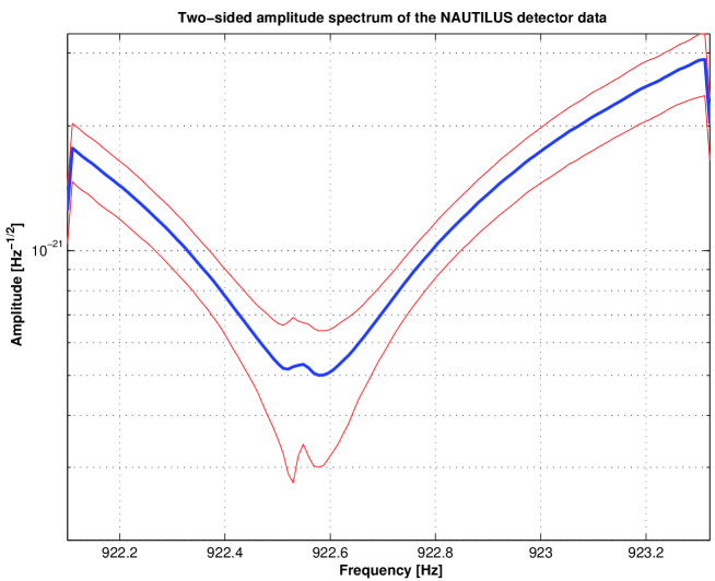
Figure 1: Estimation of the two-sided amplitude spectrum of the NAUTILUS data in the year 2001 and the rms error of the estimate. The thick line shows the estimate and the two thin lines correspond to the 1 $\sigma$ error.

During the search we have obtained $537\,665\,380$ candidates above the $2{\mathcal{F}}$-threshold of $40$ and $9\,038\,817$ above the $2{\mathcal{F}}$-threshold of $50$.

4 Analysis of the candidates

4.1 Signal-to-noise ratio of the candidates

In Figure 2 we have plotted a histogram of the frequencies of all the candidates above the $2{\mathcal{F}}$-threshold of 50. The histogram shows an excess of candidates in the frequency band of $\langle 922.4;\,922.6\rangle$ Hz. This excess is a result of the presence of a periodic interference in the data that appears as a series of harmonics in the bandwidth of the detector. One of the harmonics is located in the subband $\langle 922.2;\,923.2\rangle$ Hz. The effect of the harmonic is visible in our estimate of the spectrum (Figure 1) and appears as a bump in the band $\langle 922.5;\,922.6\rangle$ Hz.

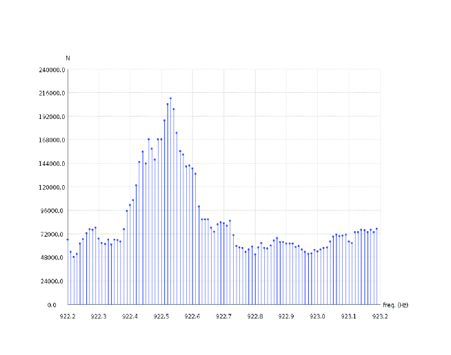
Figure 2: Histogram of the frequencies of candidates obtained in the search of all 93 two day data stretches above a $2{\mathcal{F}}$-threshold of 50.

As a first step in the candidate analysis we have calculated the increase in signal-to-noise ratio when we increase the observation time from two to four days. This has been done for all the candidates above the threshold $2{\mathcal{F}}=50$. Figure 3 shows the highest increase in SNR for candidates when going from a two day data stretch to the four day one. The maximum is calculated for each of the 93 data stretches analyzed.

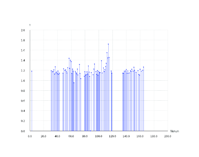
Figure 3: Highest increase (vertical axis) in signal-to-noise ratio for candidates in each of the 93 data stretches analyzed. The two day stretches of Nautilus 2001 data are numbered form 1 to 182. The missing lines in the plot indicate that the corresponding data stretch was not analyzed.

We see that typically the highest gain in the signal-to-noise is $1.2$. This should be compared with the theoretical gain of $\sqrt{2}$ of SNR when we increase the observation time by a factor of 2. The periodic interference present in the data to which we attribute these maximum SNR increases does not gives a higher increase of the SNR because its frequency changes erratically over the observation time of days and it cannot reproduce the Doppler shift of a real GW signal modulated by detector motion with respect to the SSB. Assuming that the two day sequence is independent of the four day sequence we could perform the $F$-test that consists of calculation of the ratio $F$ of the ${\mathcal{F}}$-statistic for 4 days observation time and the ${\mathcal{F}}$-statistic for 2 days observation time. Taking as the null hypothesis for the test that data is only Gaussian noise the $2{\mathcal{F}}$-statistic has the central $\chi^{2}$ distribution with 4-degrees of freedom and the ratio $F$ has Fisher-Snedeckor distribution $F(4,4)$. The typical highest value of $F$ for a given data segment is around $1.5$ The probability of $F$ crossing the threshold $1.5$ is around $37$%. This would give a high confidence that data is noise only. Unfortunately this is only a crude approximation because the two day sequence is contained in the four day one and the assumption of independence of the two ${\mathcal{F}}$-statistic is not fulfilled.

4.2 Coincidences among the candidates from different data stretches

Candidates from different data stretches are considered coincident if they cluster closely together in the four-dimensional parameter space $(\omega_{0},\omega_{1},\delta,\alpha)$. We employ the clustering method described in [14], which uses a grid of “coincidence cells”. This method will reliably detect strong signals which would produce candidates with closely-matched parameters in many of the different data stretches.

In a first step, the frequency value of each candidate above the threshold of $2{\mathcal{F}}=40$ is shifted to the same fiducial time: the GPS start time of the earliest ($j=1$) stretch, $t_{\rm fiducial}=t_{1}=662\,547\,735.9988098\,{\rm s}$. Defining $T_{0}$ to be the time span of two sidereal days, the frequencies of the candidates are shifted to $t_{\rm fiducial}$ via

$$\omega_{0}(t_{\rm fiducial})=\omega_{0}(t_{j})+(j-1)\,2\omega_{1}T_{0},$$ (16)

where $t_{j}$ is the starting time of the $j$’th data stretch, given by $t_{j}=t_{\rm fiducial}+(j-1)\,T_{0}$.

To find coincidences, a grid of cells is constructed such that the cells are rectangular in the coordinates $(\omega_{0},\omega_{1},\delta,\alpha\cos\delta)$. The dimensions of the cells are adapted to the parameter space search. Thus, the cells are constructed to be as small as possible to reduce the probability of coincidences due to false alarms. However, since each of the 93 different data stretches uses a slightly different parameter space grid, the coincidence cells must be chosen to be large enough that the candidates from a source (which would appear at slightly different points in parameter space in each of the 93 data stretches) would still lie in the same coincidence cell. As a conservative choice we use cell sizes in $\omega_{0}$ of $5.8\times 10^{-4}\,{\rm Hz}$, in $\omega_{1}$ of $2.08\times 10^{-11}\,{\rm Hz\,s^{-1}}$, and an isotropic cell grid in the sky with equatorial spacing of $0.028\,{\rm rad}$. Each candidate event is assigned to a particular cell. In cases where two or more candidate events from the same data stretch $j$ fall into the same cell, only the candidate having the largest value of $2{\mathcal{F}}$ is retained in the cell. Then the number of candidate events per cell coming from distinct data stretches is counted.

From the 93 different data stretches, this coincidence method found that we get candidates which appear consistently in no more than 4 data stretches uniformly over the search bandwidth, where there are no instrumental interferences. This is the background of the number of coincidences. We would like to test the null hypothesis that the coincidences are result of the noise only. Let us assume that the parameter space is divided into $N_{cell}$ independent coincidence cells, the candidate events are independent and the probability for a candidate event to fall into any given coincidence cell is $1=1/N_{cell}$. Thus probability $\epsilon$ that a given coincidence cell is populated with one or more candidate event is given by

$$\epsilon=1-(1-\frac{1}{N_{cell}})^{\varepsilon_{seg}},$$ (17)

where $\varepsilon_{seg}$ is the number of candidate events per data segment. The probability $p_{F}$ that any given coincidence cell contains candidate events from ${\mathcal{C}}_{max}$ or more distinct data segments is given by a binomial distribution

$$p_{F}=\sum^{N_{seg}}_{n={\mathcal{C}}_{max}}{N_{seg}\choose n}\epsilon^{n}(1-\epsilon)^{N_{seg}-n}.$$ (18)

Finally the probability $P_{F}$ that there is ${\mathcal{C}}_{max}$ or more coincidences in one or more of the $N_{cell}$ cells is

$$P_{F}=1-(1-p_{F})^{N_{cell}}.$$ (19)

The expected number of cells with ${\mathcal{C}}_{max}$ or more coincidences is given by

$$N_{F}=N_{cell}\,p_{F}.$$ (20)

In our case the number of cells is given by $N_{cell}=5.9\times 10^{10}$, the number of data segments is $N_{seg}=93$, and the number of candidates per data segment is $\varepsilon_{seg}=5.8\times 10^{6}$. From Equation (19) we find that the probability of finding ${\mathcal{C}}_{max}=4$ or more coincident candidates is almost one. Thus for the background coincidences we can accept the null hypothesis that they are from noise only with a high confidence. Over the bandwidth $\langle 922.4;\,922.6\rangle$ Hz we find an excess of coincidences with the maximum of 8 coincidences. By Equation (19), the false alarm probability associated with with 8 or more coincidences is of the order of $10^{-11}$ and thus they cannot be attributed to noise. We consider these coincidences to be due to the periodic interference present in the data.

5 Upper limits

Our verification procedure consisting of coincidences among the candidates from distinct data segments and an analysis of the increase of signal-to-noise ratio presented in section 4 did not produce convincing evidence of a gravitational-wave signal. We therefore proceeded to estimate the upper limits for the amplitudes of the gravitational-wave signals in the parameter space that we have searched. Detection of a signal is signified by a large value of the ${\mathcal{F}}$-statistic that is unlikely to arise from the noise-only distribution. If instead the value of ${\mathcal{F}}$ is consistent with pure noise with high probability we can place an upper limit on the strength of the signal. One way of doing this is to take the loudest event obtained in the search and solve the equation

$${\cal P}=P_{D}(\rho_{\mathrm{ul}},{\mathcal{F}}_{\mathrm{loudest}})$$ (21)

for signal-to-noise ratio $\rho_{\mathrm{ul}}$, where $P_{D}$ is the detection probability, ${\mathcal{F}}_{\mathrm{loudest}}$ is the value of the ${\mathcal{F}}$-statistic corresponding to the loudest event, and ${\cal P}$ is a chosen confidence. Then $\rho_{\mathrm{ul}}$ is the desired upper limit with confidence ${\cal P}$. We can also obtain an upper limit $\rho_{\mathrm{ul}}$ with confidence ${\cal P}$ for several independent searches from the equation

$${\cal P}=1-\prod^{L}_{s=1}\left[1-P_{D}(\rho_{\mathrm{ul}},{\mathcal{F}}_{\mathrm{loudest}\,s})\right],$$ (22)

where ${\mathcal{F}}_{\mathrm{loudest}\,s}$ is the threshold corresponding to the loudest event in $s$’th search and $L$ is the number of searches. Here ${\cal P}$ is the probability that a signal with signal-to-noise ratio $\rho_{\mathrm{ul}}$ crosses the threshold ${\mathcal{F}}_{\mathrm{loudest}\,s}$ in at least one of the $L$ independent searches. To calculate $\rho_{\mathrm{ul}}$ we assume that the data have a Gaussian distribution and consequently the probability of detection $P_{D}$ has a non-central $\chi^{2}$ distribution with 4 degrees of freedom and the noncentrality parameter equal to $\rho^{2}_{\mathrm{ul}}$ . We have investigated this assumption by obtaining histograms of the $2{\mathcal{F}}$-statistic values of the candidates and comparing them to the central $\chi^{2}$ distribution with 4 degrees of freedom. The result is shown in Figure 4. There is an overall qualitative agreement of candidates distributions with the theoretical one. However, the candidates distributions do not pass a goodness-of-fit test for a $\chi^{2}$ distribution at the significance level of 5%.

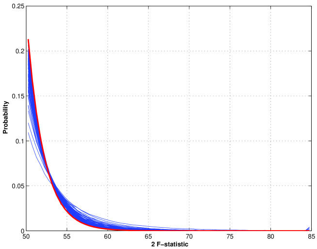
Figure 4: Probability distribution of $2{\mathcal{F}}$-statistic values of the candidates. The light lines are obtained from histograms of the $2{\mathcal{F}}$ values of each data segment. The thick line represents the theoretical central $\chi^{2}$ distribution with 4 degrees of freedom.

In order to translate our upper limit on the SNR into the upper limit on the gravitational-wave amplitude, we use the Equation (93) of [2] for signal-to-noise ratio of a GW signal from a spinning neutron star averaged over the source position and orientation. Thus $h_{\mathrm{ul}}$ and $\rho_{\mathrm{ul}}$ are related by the following formula:

$$h_{\mathrm{ul}}(f)=\frac{5}{2}\sqrt{\frac{S(f)}{T_{0}}}\rho_{\mathrm{ul}},$$ (23)

where $S(f)$ is one-sided spectral density at frequency $f$. We have used Equations (22) and (23) to obtain upper limits in $0.1$ Hz bands over the bandwidth $\langle 922.2;\,923.2\rangle$ Hz that we have searched. The upper limit results are presented in Figure 5. Assumed Gaussian noise, we have chosen the confidence ${\cal P}=90\%$ and we denote the upper limits by $h_{o}^{90\%}$.

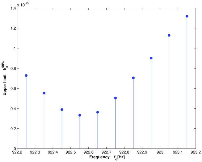
Figure 5: Upper limits based on the loudest candidate for 0.1 Hz frequency bands over the 1 Hz bandwidth searched.

Our best upper limit is equal to $3.4\times 10^{-23}$ at a frequency of 922.55 Hz. Using our 1 $\sigma$ rms error of the amplitude power spectrum estimate we reckon that our upper limit has likewise an error of $18$%.

References

References

- [1] Astone P et al(ROG Collaboration) 1997 Astroparticle Physics 7 231-243
- [2] Jaranowski P, Królak A and Schutz B F 1998 Phys. Rev. D 58 063001
- [3] Jaranowski P and Królak A 2005 Living Rev. Relativity 8 3
- [4] Mauceli et al2000 arXiv:gr-qc/0007023v1
- [5] Astone P et al2002 Phys. Rev. D 65 022001
- [6] Astone P et al2003 Class. Quantum Grav. 20 S665–S676
- [7] Astone P et al2005 Class. Quantum Grav. 22 S1243–S1254
- [8] Abbott B et al(LIGO Scientific Collaboration) 2004 Phys. Rev. D 69 082004
- [9] Abbott B et al(LIGO Scientific Collaboration), Kramer M and Lyne A 2005 Phys. Rev. Lett. 94 181103
- [10] Abbott B et al(LIGO Scientific Collaboration), Kramer M and Lyne A 2007 Phys. Rev. D 76 042001
- [11] Abbott B et al(LIGO Scientific Collaboration) 2007 Phys. Rev. D 76 082001
- [12] Abbott B et al(LIGO Scientific Collaboration) 2005 Phys. Rev. D 72 102004
- [13] Abbott B et al(LIGO Scientific Collaboration) 2008 Phys. Rev. D 77 022001
- [14] LIGO Scientific Collaboration 2008 The Einstein@Home search for periodic gravitational waves in LIGO S4 data Preprint arXiv:0804.1747v1 [gr-qc]
- [15] Astone P, Borkowski K M, Jaranowski P and Królak A 2002 Phys. Rev. D 65 042003
- [16] Conway J H and Sloane N J A 1993 Sphere Packings, Lattices and Groups (New York: Springer-Verlag)
- [17] Prix R 2007 Class. Quantum Grav.24 S481–S490
- [18] Schutz B F 1991 The Detection of Gravitational Waves ed D G Blair (Cambridge: Cambridge University Press) pp 406–452
- [19] Jaranowski P and Królak A 1999 Phys. Rev. D 59 063003
- [20] Jaranowski P and Królak A 2000 Phys. Rev. D 61 062001
- [21] Brady P R, Creighton T, Cutler C and Schutz B F 1998 Phys. Rev. D 57 2101
- [22] Owen B 1996 Phys. Rev. D 53 6749