Large-scale magnetic topologies of early M dwarfs

Abstract

We present here additional results of a spectropolarimetric survey of a small sample of stars ranging from spectral type M0 to M8 aimed at investigating observationally how dynamo processes operate in stars on both sides of the full convection threshold (spectral type M4).

The present paper focuses on early M stars (M0–M3), i.e. above the full convection threshold. Applying tomographic imaging techniques to time series of rotationally modulated circularly polarised profiles collected with the NARVAL spectropolarimeter, we determine the rotation period and reconstruct the large-scale magnetic topologies of 6 early M dwarfs. We find that early-M stars preferentially host large-scale fields with dominantly toroidal and non-axisymmetric poloidal configurations, along with significant differential rotation (and long-term variability); only the lowest-mass star of our subsample is found to host an almost fully poloidal, mainly axisymmetric large-scale field ressembling those found in mid-M dwarfs.

This abrupt change in the large-scale magnetic topologies of M dwarfs (occuring at spectral type M3) has no related signature on X-ray luminosities (measuring the total amount of magnetic flux); it thus suggests that underlying dynamo processes become more efficient at producing large-scale fields (despite producing the same flux) at spectral types later than M3. We suspect that this change relates to the rapid decrease in the radiative cores of low-mass stars and to the simultaneous sharp increase of the convective turnover times (with decreasing stellar mass) that models predict to occur at M3; it may also be (at least partly) responsible for the reduced magnetic braking reported for fully-convective stars.

1 Introduction

Activity and magnetic fields are ubiquitous to cool stars of all spectral types (e.g., Saar & Linsky, 1985; Donati et al., 1997). The analogy with the Sun suggests that these fields are produced through dynamo mechanisms operating in a thin interface layer at the base of the convective envelope, where angular rotation gradients are strongest. Starting from a weak poloidal configuration, differential rotation progressively winds the field around the star, building a strong toroidal belt at the base of the convective zone; cyclonic turbulence then restores a weak poloidal field (with a polarity opposite to that of the initial one) once the toroidal field has grown unstable (Parker, 1955). However, there is still considerable controversy (even for the Sun itself) on how and where exactly the field is amplified and on which physical processes (differential rotation, meridional circulation) are mainly controlling the magnetic cycle (e.g., Charbonneau, 2005).

Observing stars other than the Sun is of obvious interest for this question as they provide a direct way of studying how dynamo processes depend on fundamental stellar parameters such as mass (and thus convective depth) and rotation rate. In this respect, low-mass fully-convective stars are particularly interesting as they host no interface layer (where dynamo processes presumably concentrate in the Sun), and nevertheless show both strong magnetic fields (e.g., Johns-Krull & Valenti, 1996) and intense activity (e.g., Delfosse et al., 1998). Many theoretical models were proposed to attempt resolving this issue (e.g., Durney et al., 1993; Dobler et al., 2006; Browning, 2008) but observations of the large-scale magnetic fields at the surfaces of fully-convective stars, and in particular of their poloidal and toroidal components, are still rare.

Thanks to time-resolved spectropolarimetric observations of cool stars, we are now able to recover information on how magnetic fields distribute at (and emerge from) the surfaces of cool active stars (e.g., Donati et al., 2003a). With the advent of new generation instruments optimised in this very purpose (ESPaDOnS at the 3.6m Canada-France-Hawaii Telescope and NARVAL at the 2m Télescope Bernard Lyot in France, Donati, 2003), this technique can now be also applied to faint M dwarfs. The first attempt focussed on the fully-convective rapidly-rotating M4 star V374 Peg and revealed that, against all theoretical expectations, fully-convective M dwarfs are apparently very efficient at producing strong large-scale mainly-axisymmetric poloidal fields (Donati et al., 2006a) despite very small levels of differential rotation. A follow-up study confirmed this point and further demonstrated that the magnetic configuration of V374 Peg is apparently stable on timescales of $\simeq 1$ yr (Morin et al., 2008a).

To investigate this issue in more details, we embarked in a spectropolarimetric survey of a small sample of M dwarfs, located both above and below the full-convection threshold (corresponding to a mass of 0.35 ${\rm M}_{\odot}$ and to a spectral type of M4). The first results of this survey, focussing mainly on active M4 dwarfs, confirms the results obtained on V374 Peg and demonstrate that strong large-scale mainly-axisymmetric poloidal fields are indeed fairly common in fully-convective mid-M active dwarfs (Morin et al., 2008b, hereafter M08). In this new paper, we present the results for the 6 early M dwarfs that we observed in this survey, namely DT Vir, DS Leo, CE Boo, OT Ser, GJ 182 and GJ 49, with spectral types ranging from M0 to M3 (see Table 1). After briefly describing the observations and the magnetic modelling method that we use, we detail the results obtained for each star and discuss their implication for our understanding of dynamo processes in cool active stars.

Table 1: Fundamental parameters of our sample early-M dwarf stars. Columns 1 to 6 respectively list the name, the spectral type, the mass $M_{\star}$ (derived from the Hipparcos distance and the J, H and K magnitudes using the mass-luminosity relations of Delfosse et al. 2000 except for GJ 182; for which we used the evolutionary models of Baraffe et al. 1998, see text), the logarithmic bolometric luminosity $\log L_{\rm bol}$ (derived from the mass and the models of Baraffe et al. 1998), the logarithmic relative X-ray luminosity $\log R_{\rm X}$ (i.e., $\log L_{\rm X}/L_{\rm bol}$, from Kiraga & Stepien 2007 or from the NEXXUS data base, Schmitt & Liefke 2004, or from Wood et al. 1994 for GJ 49), the projected rotation velocity (this paper, accuracy $\simeq 1$ km s^-1), the rotation period (this paper), the convective turnover time $\tau_{\rm c}$ (from Kiraga & Stepien 2007), the effective Rossby number $Ro=\hbox{$P_{\rm rot}$}/\tau_{\rm c}$, the radius $R_{\star}$ (predicted by the theoretical models of Baraffe et al. 1998) and the assumed inclination angle of the rotation axis to the line-of-sight (this paper).

Star	ST	$M_{\star}$	$\log L_{\rm bol}$	$\log R_{\rm X}$	$v\sin i$	$P_{\rm rot}$	$\tau_{\rm c}$	$Ro$	$R_{\star}$	$i$
		(${\rm M}_{\odot}$)	(erg s-1)		(km s-1)	(d)	(d)		(${\rm R}_{\odot}$)	(∘)
GJ 182	M0.5	0.75	32.7	–3.1	10	4.35	25	0.174	0.82	60
DT Vir / GJ 494A	M0.5	0.59	32.3	–3.4	11	2.85	31	0.092	0.53	60
DS Leo / GJ 410	M0	0.58	32.3	–4.0	2	14.0	32	0.438	0.52	60
GJ 49	M1.5	0.57	32.3	$<-4.3$	1	18.6	33	0.564	0.51	45
OT Ser / GJ 9520	M1.5	0.55	32.2	–3.4	6	3.40	35	0.097	0.49	45
CE Boo / GJ 569A	M2.5	0.48	32.1	–3.7	1	14.7	42	0.350	0.43	45

2 Observations

Spectropolarimetric observations of the selected M dwarfs were collected with NARVAL and the 2m Télescope Bernard Lyot (TBL), between 2007 Jan and 2008 Feb (in 3 different runs). NARVAL is a twin spectropolarimeter copied from ESPaDOnS (Donati, 2003), yielding full coverage of the optical domain (370 to 1000 nm) at a resolving power of about 65 000 in a single exposure. Each polarisation exposure consists of 4 individual subexposures taken in different polarimeter configurations and combined together to filter out all spurious polarisation signatures at first order (e.g., Donati et al., 1997).

Data reduction was carried out using Libre ESpRIT, a fully automated package/pipeline installed at TBL and performing optimal extraction of unpolarised (Stokes $I$) and circularly polarised (Stokes $V$) spectra as described in Donati et al. (1997). The peak signal-to-noise ratios (S/N) per 2.6 km s^-1 velocity bin that we obtained in the collected spectra range from 100 to 400 depending on the magnitude and weather conditions. The journal of observations for all stars is presented in Tables 2 to 7.

All spectra are automatically corrected from spectral shifts resulting from instrumental effects (eg mechanical flexures, temperature or pressure variations) using telluric lines as a reference. Though not perfect, this procedure allows spectra to be secured with a radial velocity (RV) precision of better than 0.030 km s^-1 (e.g., Moutou et al., 2007).

Table 2: Journal of observations for DT Vir=GJ 494A. Columns 1–7 list the UT date, the heliocentric Julian date, the UT time, the total exposure time, the peak signal to noise ratio (per 2.6 km s^-1 velocity bin) and the rms noise level in the LSD Stokes $V$ profile (relative to the unpolarised continuum level and per 1.8 km s^-1 velocity bin). In col. 8 and 9, we list the rotational cycles (using ephemeris HJD$=2,454,100.0+2.85E$) as well as the longitudinal fields $B_{\rm\ell}$ (with error bars) and the radial velocities $v_{\rm r}$ (absolute accuracy 0.10 km s^-1, internal accuracy 0.03 km s^-1) associated to each exposure.

Date	HJD	UT	$t_{\rm exp}$	S/N	$\sigma_{\rm LSD}$	Cycle	$B_{\rm\ell}$	$v_{\rm r}$
	(2,454,000+)	(h:m:s)	(s)		($10^{-4}I_{\rm c}$)		(G)	(km s-1)
2007 Jan 26	126.70173	04:47:56	4$\times 800$	240	3.3	9.369	$-17.6\pm 9.3$	$-13.32$
Jan 27	127.67710	04:12:22	4$\times 800$	310	2.3	9.711	$-3.8\pm 6.7$	$-13.44$
Jan 28	128.69001	04:30:50	4$\times 800$	350	2.0	10.067	$66.0\pm 5.8$	$-13.04$
Jan 29	129.65374	03:38:29	4$\times 800$	340	2.1	10.405	$-27.6\pm 6.0$	$-13.29$
Feb 02	133.71569	05:07:13	4$\times 800$	350	2.0	11.830	$23.3\pm 5.7$	$-13.29$
Feb 03	134.69961	04:43:57	4$\times 800$	340	2.1	12.175	$49.7\pm 6.0$	$-13.00$
Feb 04	135.71225	05:02:02	4$\times 800$	360	1.9	12.531	$-31.1\pm 5.6$	$-13.32$
Feb 05	136.66208	03:49:41	2$\times 800$	140	5.2	12.864	$28.0\pm 15.5$	$-13.25$
2007 Dec 28	462.71536	05:11:18	4$\times 750$	330	2.2	127.269	$30.5\pm 6.5$	$-13.64$
Dec 29	463.74605	05:55:22	4$\times 750$	360	2.0	127.630	$15.5\pm 5.7$	$-13.67$
Dec 31	465.74401	05:52:10	4$\times 700$	290	2.5	128.331	$29.0\pm 7.1$	$-13.66$
2008 Jan 01	466.74583	05:54:39	4$\times 700$	360	2.0	128.683	$24.5\pm 5.7$	$-13.69$
Jan 19	484.63507	03:12:52	4$\times 600$	170	4.5	134.960	$26.3\pm 12.8$	$-13.57$
Jan 20	485.61280	02:40:40	4$\times 600$	200	4.0	135.303	$29.4\pm 11.3$	$-13.77$
Jan 23	488.62610	02:59:27	4$\times 600$	250	3.1	136.360	$23.6\pm 9.0$	$-13.74$
Jan 24	489.62041	02:51:08	4$\times 600$	240	2.9	136.709	$1.5\pm 8.6$	$-13.65$
Jan 26	491.60391	02:27:08	4$\times 600$	230	3.3	137.405	$39.8\pm 9.5$	$-13.69$
Jan 27	492.62606	02:58:54	4$\times 600$	320	2.2	137.763	$-4.5\pm 6.2$	$-13.67$
Jan 28	493.63758	03:15:22	4$\times 600$	300	2.4	138.118	$4.5\pm 6.7$	$-13.56$
Feb 03	499.63751	03:14:34	4$\times 600$	280	2.7	140.224	$8.9\pm 7.7$	$-13.80$
Feb 05	501.64773	03:29:03	4$\times 600$	290	2.4	140.929	$53.9\pm 7.0$	$-13.59$
Feb 06	502.63636	03:12:34	4$\times 600$	320	2.2	141.276	$-7.1\pm 6.4$	$-13.75$
Feb 07	503.64038	03:18:15	4$\times 600$	290	2.4	141.628	$23.2\pm 7.1$	$-13.69$
Feb 10	506.64784	03:28:40	4$\times 600$	310	2.3	142.684	$7.0\pm 6.6$	$-13.65$
Feb 12	508.63939	03:16:18	4$\times 600$	300	2.4	143.382	$-4.9\pm 6.9$	$-13.82$
Feb 14	510.63942	03:16:08	4$\times 600$	230	3.2	144.084	$7.4\pm 9.2$	$-13.61$
Feb 15	511.65542	03:39:04	4$\times 600$	280	2.5	144.440	$6.7\pm 7.3$	$-13.77$
Feb 16	512.64053	03:17:32	4$\times 600$	300	2.4	144.786	$-2.0\pm 6.7$	$-13.68$
Feb 17	513.64033	03:17:09	4$\times 600$	310	2.3	145.137	$-0.1\pm 6.6$	$-13.65$

Table 3: Same as Table 2 for DS Leo=GJ 410. Rotational cycles are now computed using ephemeris HJD$=2,454,100.0+14.0E$.

Date	HJD	UT	$t_{\rm exp}$	S/N	$\sigma_{\rm LSD}$	Cycle	$B_{\rm\ell}$	$v_{\rm r}$
	(2,454,000+)	(h:m:s)	(s)		($10^{-4}I_{\rm c}$)		(G)	(km s-1)
2007 Jan 26	126.65015	03:31:14	4$\times 800$	250	2.7	1.904	$-33.9\pm 4.1$	$-14.08$
Jan 27	127.63491	03:09:13	4$\times 800$	270	2.3	1.974	$-15.9\pm 3.4$	$-14.05$
Jan 28	128.64692	03:26:27	4$\times 800$	320	2.0	2.046	$-1.3\pm 3.0$	$-14.08$
Jan 29	129.61070	02:34:13	4$\times 800$	330	1.9	2.115	$13.1\pm 2.9$	$-14.06$
Jan 30	130.65362	03:35:57	4$\times 800$	340	1.7	2.189	$29.7\pm 2.6$	$-14.08$
Feb 02	133.67041	03:59:57	4$\times 800$	340	1.8	2.405	$6.3\pm 2.8$	$-14.03$
Feb 03	134.65677	03:40:15	4$\times 800$	340	1.8	2.475	$7.0\pm 2.8$	$-14.01$
Feb 04	135.66947	03:58:28	4$\times 800$	350	1.8	2.548	$3.7\pm 2.7$	$-14.02$
Feb 05	136.63031	03:02:02	4$\times 800$	200	3.2	2.617	$2.4\pm 5.1$	$-14.04$
2007 Dec 28	462.67598	04:11:04	4$\times 750$	320	2.0	25.905	$9.9\pm 2.9$	$-14.09$
Dec 29	463.70487	04:52:33	4$\times 750$	340	1.8	25.979	$1.5\pm 2.7$	$-14.09$
Dec 31	465.70955	04:59:06	4$\times 600$	260	2.5	26.122	$8.6\pm 3.7$	$-14.08$
2008 Jan 01	466.70912	04:58:22	4$\times 700$	350	1.8	26.194	$24.5\pm 2.7$	$-14.09$
Jan 02	467.68306	04:20:44	2$\times 600$	130	5.1	26.263	$13.9\pm 7.7$	$-14.07$
Jan 03	468.70748	04:55:48	4$\times 700$	180	3.8	26.336	$26.9\pm 5.6$	$-14.05$
Jan 07	472.62578	02:57:46	4$\times 700$	160	4.3	26.616	$-22.1\pm 7.0$	$-14.06$
Jan 08	473.62319	02:53:56	4$\times 700$	260	2.4	26.687	$-4.0\pm 3.9$	$-14.11$
Jan 19	484.58050	01:51:30	4$\times 600$	180	4.0	27.470	$-17.2\pm 5.9$	$-14.04$
Jan 20	485.55637	01:16:40	4$\times 600$	190	3.7	27.540	$-26.8\pm 5.5$	$-14.05$
Jan 22	487.58395	01:56:14	4$\times 600$	230	2.8	27.685	$-9.6\pm 4.4$	$-14.04$
Jan 24	489.53279	00:42:24	4$\times 600$	250	2.6	27.824	$6.4\pm 3.8$	$-14.05$
Jan 26	491.54899	01:05:35	4$\times 600$	240	2.6	27.968	$7.1\pm 3.8$	$-14.08$
Jan 27	492.57173	01:38:15	4$\times 600$	310	2.0	28.041	$-3.5\pm 3.0$	$-14.07$
Jan 28	493.58339	01:54:59	4$\times 600$	290	2.2	28.113	$6.7\pm 3.3$	$-14.04$
Feb 03	499.60160	02:20:49	4$\times 600$	270	2.3	28.543	$-22.3\pm 3.8$	$-14.11$
Feb 05	501.58341	01:54:31	4$\times 600$	250	2.6	28.684	$-0.9\pm 4.1$	$-14.08$
Feb 06	502.58201	01:52:26	4$\times 600$	310	2.1	28.756	$4.3\pm 3.1$	$-14.08$
Feb 07	503.58042	01:50:06	4$\times 600$	290	2.2	28.827	$3.5\pm 3.2$	$-14.10$
Feb 10	506.59331	02:08:31	4$\times 600$	290	2.1	29.042	$4.2\pm 3.2$	$-14.03$
Feb 11	507.55697	01:16:08	4$\times 600$	300	2.0	29.111	$5.8\pm 2.9$	$-14.06$
Feb 12	508.58557	01:57:17	4$\times 600$	310	2.2	29.185	$16.1\pm 3.3$	$-14.04$
Feb 13	509.59071	02:04:38	4$\times 600$	290	2.2	29.256	$16.1\pm 3.3$	$-14.02$
Feb 14	510.58572	01:57:25	4$\times 600$	230	2.9	29.328	$10.9\pm 4.3$	$-14.03$
Feb 15	511.60258	02:21:39	4$\times 600$	300	2.1	29.400	$-9.4\pm 3.2$	$-13.98$
Feb 16	512.58834	02:01:06	4$\times 600$	270	2.4	29.471	$-16.5\pm 3.5$	$-14.04$
Feb 17	513.58759	01:59:59	4$\times 600$	300	2.1	29.542	$-16.9\pm 3.1$	$-14.02$

Table 4: Same as Table 2 for CE Boo=GJ 569A. Rotational cycles are now computed using ephemeris HJD$=2,454,100.0+14.7E$.

Date	HJD	UT	$t_{\rm exp}$	S/N	$\sigma_{\rm LSD}$	Cycle	$B_{\rm\ell}$	$v_{\rm r}$
	(2,454,000+)	(h:m:s)	(s)		($10^{-4}I_{\rm c}$)		(G)	(km s-1)
2008 Jan 19	484.66641	04:01:44	4$\times 600$	130	6.2	26.168	$-93.6\pm 14.5$	$-7.31$
Jan 20	485.68258	04:24:54	4$\times 600$	200	3.9	26.237	$-92.2\pm 9.3$	$-7.36$
Jan 23	488.65820	03:49:27	4$\times 600$	230	3.3	26.439	$-59.3\pm 7.8$	$-7.28$
Jan 24	489.65197	03:40:21	4$\times 600$	190	3.7	26.507	$-73.3\pm 8.8$	$-7.29$
Jan 26	491.63667	03:18:05	4$\times 600$	170	4.7	26.642	$-110.2\pm 11.2$	$-7.31$
Jan 27	492.65802	03:48:42	4$\times 600$	270	2.6	26.711	$-90.5\pm 6.1$	$-7.34$
Jan 28	493.67096	04:07:12	4$\times 600$	280	2.5	26.780	$-114.2\pm 6.1$	$-7.31$
Jan 30	495.68078	04:21:06	4$\times 600$	250	2.9	26.917	$-111.0\pm 6.8$	$-7.35$
Feb 03	499.69324	04:38:34	4$\times 600$	260	2.7	27.190	$-70.4\pm 6.5$	$-7.42$
Feb 05	501.68094	04:20:37	4$\times 600$	250	2.9	27.325	$-53.8\pm 6.9$	$-7.35$
Feb 07	503.67364	04:09:51	4$\times 600$	260	2.7	27.461	$-54.9\pm 6.4$	$-7.35$
Feb 10	506.67974	04:18:16	4$\times 600$	270	2.7	27.665	$-91.0\pm 6.3$	$-7.32$
Feb 11	507.68809	04:30:10	4$\times 600$	280	2.4	27.734	$-113.4\pm 5.9$	$-7.36$
Feb 12	508.67116	04:05:40	4$\times 600$	240	3.0	27.801	$-115.0\pm 7.1$	$-7.34$
Feb 13	509.67882	04:16:35	4$\times 600$	230	3.1	27.869	$-108.6\pm 7.4$	$-7.33$
Feb 14	510.67193	04:06:32	4$\times 600$	200	3.7	27.937	$-106.7\pm 8.6$	$-7.35$
Feb 15	511.68789	04:29:24	4$\times 600$	270	2.7	28.006	$-111.7\pm 6.4$	$-7.31$
Feb 16	512.67287	04:07:39	4$\times 600$	260	2.6	28.073	$-85.5\pm 6.2$	$-7.37$
Feb 17	513.67252	04:07:02	4$\times 600$	270	2.6	28.141	$-79.9\pm 6.2$	$-7.34$

Table 5: Same as Table 2 for OT Ser=GJ 9520. Rotational cycles are now computed using ephemeris HJD$=2,454,100.0+3.40E$.

Date	HJD	UT	$t_{\rm exp}$	S/N	$\sigma_{\rm LSD}$	Cycle	$B_{\rm\ell}$	$v_{\rm r}$
	(2,454,000+)	(h:m:s)	(s)		($10^{-4}I_{\rm c}$)		(G)	(km s-1)
2007 Jul 26	308.42253	22:05:53	4$\times 900$	270	2.7	61.301	$80.0\pm 5.7$	$6.89$
Jul 28	310.38549	21:12:45	4$\times 900$	340	2.0	61.878	$55.0\pm 4.6$	$6.75$
Jul 29	311.43298	22:21:15	4$\times 900$	370	1.8	62.186	$73.4\pm 4.1$	$6.87$
Jul 30	312.41904	22:01:17	4$\times 900$	380	1.8	62.476	$74.9\pm 3.8$	$6.82$
Jul 31	313.41995	22:02:42	4$\times 900$	230	3.2	62.771	$67.0\pm 7.0$	$6.82$
Aug 02	315.42156	22:05:14	4$\times 900$	350	1.9	63.359	$80.9\pm 4.2$	$6.90$
Aug 03	316.42155	22:05:20	4$\times 900$	350	1.9	63.653	$67.8\pm 4.2$	$6.84$
Aug 04	317.42236	22:06:36	4$\times 900$	230	3.1	63.948	$55.5\pm 7.1$	$6.77$
Aug 09	322.41667	21:58:58	4$\times 900$	330	2.1	65.417	$77.7\pm 4.5$	$6.87$
Aug 10	323.41738	22:00:06	4$\times 900$	250	2.8	65.711	$70.5\pm 6.1$	$6.82$
Aug 14	327.35676	20:33:15	4$\times 900$	270	2.7	66.870	$54.5\pm 6.0$	$6.79$
2008 Jan 19	484.74579	05:56:56	4$\times 600$	150	5.2	113.160	$52.7\pm 10.6$	$6.78$
Jan 20	485.71587	05:13:45	4$\times 600$	190	3.9	113.446	$1.4\pm 8.1$	$6.80$
Jan 23	488.69155	04:38:25	4$\times 600$	180	4.1	114.321	$8.9\pm 8.7$	$6.81$
Jan 24	489.68897	04:34:36	4$\times 600$	160	4.5	114.614	$69.1\pm 9.6$	$6.76$
Jan 26	491.67101	04:08:31	4$\times 600$	200	3.6	115.197	$47.5\pm 7.6$	$6.78$
Jan 27	492.69173	04:38:14	4$\times 600$	260	2.8	115.498	$22.4\pm 5.8$	$6.79$
Jan 28	493.70473	04:56:51	4$\times 600$	280	2.4	115.796	$90.9\pm 5.3$	$6.81$
Jan 30	495.71492	05:11:18	4$\times 600$	250	2.8	116.387	$-6.6\pm 5.9$	$6.80$
Feb 03	499.72743	05:28:51	4$\times 600$	240	2.9	117.567	$47.7\pm 6.2$	$6.72$
Feb 05	501.71560	05:11:36	4$\times 600$	260	2.7	118.152	$86.3\pm 5.7$	$6.71$
Feb 07	503.70655	04:58:20	4$\times 600$	280	2.5	118.737	$79.7\pm 5.4$	$6.75$
Feb 10	506.71299	05:07:16	4$\times 600$	260	2.7	119.621	$52.6\pm 5.6$	$6.77$
Feb 11	507.72197	05:20:05	4$\times 600$	280	2.5	119.918	$108.3\pm 5.4$	$6.71$
Feb 12	508.70420	04:54:23	4$\times 600$	240	3.0	120.207	$56.9\pm 6.2$	$6.75$
Feb 13	509.62257	02:56:43	4$\times 600$	230	3.1	120.477	$9.8\pm 6.6$	$6.78$
Feb 13	509.75390	06:05:49	4$\times 600$	270	2.6	120.516	$27.8\pm 5.5$	$6.77$
Feb 14	510.70531	04:55:45	4$\times 600$	220	3.3	120.796	$92.5\pm 6.8$	$6.78$
Feb 15	511.72139	05:18:47	4$\times 600$	270	2.5	121.094	$104.7\pm 5.4$	$6.73$
Feb 16	512.70638	04:57:03	4$\times 600$	280	2.5	121.384	$10.3\pm 5.4$	$6.74$
Feb 17	513.70577	04:56:03	4$\times 600$	270	2.5	121.678	$76.0\pm 5.4$	$6.77$

Table 6: Same as Table 2 for GJ 182. Rotational cycles are now computed using ephemeris HJD$=2,454,100.0+4.35E$.

Date	HJD	UT	$t_{\rm exp}$	S/N	$\sigma_{\rm LSD}$	Cycle	$B_{\rm\ell}$	$v_{\rm r}$
	(2,454,000+)	(h:m:s)	(s)		($10^{-4}I_{\rm c}$)		(G)	(km s-1)
2007 Jan 21	122.37018	20:48:02	4$\times 900$	210	3.2	5.143	$-84.4\pm 8.0$	$19.23$
Jan 26	127.28464	18:45:22	4$\times 900$	190	3.6	6.272	$-40.6\pm 9.2$	$19.22$
Jan 27	128.28237	18:42:12	4$\times 900$	240	2.6	6.502	$-37.9\pm 6.4$	$19.59$
Jan 30	131.27339	18:29:36	2$\times 900$	55	12.7	7.189	$-65.3\pm 36.4$	$19.22$
Feb 01	133.29669	19:03:23	4$\times 900$	250	2.4	7.654	$18.6\pm 5.9$	$19.66$
Feb 03	135.28638	18:48:47	4$\times 900$	190	3.4	8.112	$-84.2\pm 8.7$	$19.21$
Feb 08	140.29936	19:08:04	4$\times 900$	250	2.5	9.264	$-42.6\pm 6.5$	$19.24$

Table 7: Same as Table 2 for GJ 49. Rotational cycles are now computed using ephemeris HJD$=2,454,300.0+18.6E$.

Date	HJD	UT	$t_{\rm exp}$	S/N	$\sigma_{\rm LSD}$	Cycle	$B_{\rm\ell}$	$v_{\rm r}$
	(2,454,000+)	(h:m:s)	(s)		($10^{-4}I_{\rm c}$)		(G)	(km s-1)
2007 Jul 27	308.61963	02:49:20	4$\times 900$	330	2.1	0.463	$-4.6\pm 4.1$	$-6.00$
Jul 28	309.63521	03:11:41	4$\times 900$	450	1.5	0.518	$-12.0\pm 2.8$	$-6.02$
Jul 29	310.63481	03:10:59	4$\times 900$	410	1.6	0.572	$-20.9\pm 3.1$	$-6.02$
Jul 30	311.63656	03:13:25	4$\times 700$	370	1.8	0.626	$-28.4\pm 3.5$	$-6.01$
Jul 31	312.63031	03:04:19	4$\times 700$	380	1.7	0.679	$-29.2\pm 3.3$	$-6.06$
Aug 01	313.63144	03:05:51	4$\times 700$	300	2.2	0.733	$-21.7\pm 4.3$	$-6.01$
Aug 03	315.63927	03:16:55	4$\times 700$	320	2.5	0.841	$-5.9\pm 5.6$	$-6.02$
Aug 04	316.63804	03:15:03	4$\times 700$	380	1.7	0.894	$-1.6\pm 3.4$	$-6.04$
Aug 05	317.60746	02:30:56	4$\times 700$	350	1.9	0.947	$2.9\pm 3.7$	$-6.01$
Aug 09	321.61210	02:37:15	4$\times 700$	340	2.0	1.162	$-10.2\pm 3.7$	$-6.02$
Aug 10	322.63155	03:05:10	4$\times 700$	330	2.1	1.217	$-10.6\pm 3.9$	$-6.02$
Aug 11	323.63437	03:09:08	4$\times 700$	280	2.5	1.271	$-16.4\pm 4.7$	$-6.04$
Aug 15	327.62517	02:55:34	4$\times 700$	350	2.0	1.485	$-10.3\pm 3.8$	$-6.03$
Aug 18	330.61820	02:45:17	4$\times 700$	370	1.8	1.646	$-28.1\pm 3.5$	$-6.03$
Aug 19	331.57357	01:40:56	4$\times 700$	340	1.9	1.698	$-20.2\pm 3.6$	$-6.06$
Aug 31	343.56027	01:20:59	4$\times 700$	280	2.4	2.342	$-5.9\pm 4.7$	$-6.00$

Least-squares deconvolution (LSD, Donati et al., 1997) was applied to all spectra to extract the polarisation signal from most photospheric atomic lines and compute a mean Zeeman signature corresponding to an average photospheric profile (centred at 700 nm and with an effective Landé factor of 1.2). The line list used in this process is derived from an Atlas9 local thermodynamic equilibrium model (Kurucz, 1993) matching the properties of our sample, and includes about 5,000 moderate to strong atomic lines (i.e., with a relative depth larger than 40% prior to any macroscopic broadening). The resulting multiplex gain in S/N is about 15 (see Table 2). Zeeman signatures are detected in most cases on all stars. Radial velocities are obtained from Gaussian fits to all LSD unpolarised profiles. Average unpolarised LSD profiles of all stars are shown in Fig. 1.

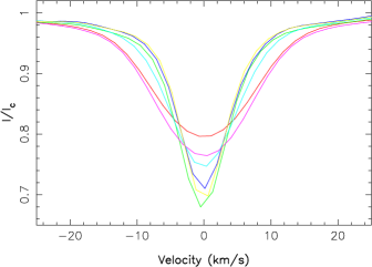
Figure 1: Average unpolarised LSD profiles for DT Vir (red line), DS Leo (green), CE Boo (dark blue), OT Ser (light blue), GJ 182 (pink) and GJ 49 (yellow). All profiles are centred on the rest velocity.

3 Magnetic modelling

The magnetic model we use to describe the time series of rotationally modulated LSD Stokes $V$ profiles is described in M08. We recall it briefly here and refer the reader to M08 for further details.

To describe the magnetic field, we use the same description as Donati et al. (2006b). The field is decomposed into its poloidal and toroidal components, both expressed as spherical harmonics expansions. The imaging process is based on the principles of maximum entropy image reconstruction, with entropy (i.e., quantifying the amount of reconstructed information) being calculated from the coefficients of the spherical harmonics expansions. Starting from a null magnetic field, we iteratively improve our magnetic model by comparing the synthetic Stokes $V$ profiles with the observed ones, until we reach an optimal field topology that reproduces the data at a given $\chi^{2}$ level (i.e., usually down to noise level, corresponding to a unit reduced $\chi^{2}$ level $\hbox{$\chi^{2}_{\nu}$}=1$). The inversion problem being partly ill-posed, we use the entropy function to select the magnetic field with lowest information content among all those reproducing the data equally well. Given that most stars considered here rotate no more than moderately, we limit spherical harmonics expansions to $\ell<10$, usually up to 8 for moderate rotators (e.g., DT Vir) and up to 5 only for the slower ones. In all cases (even the slowest rotators), we need to set $\ell>3$ to reproduce successfully the data at noise level.

To compute the synthetic profiles corresponding to a given magnetic topology, we divide the surface of the star into a grid of elementary surface cells (typically 5,000), in which the 3 components of the magnetic field (in spherical coordinates) are estimated directly from the spherical harmonics expansions used to describe the field. Using Unno-Rachkovsky’s equations (e.g., Landi degl’Innocenti, 1992), we compute the contribution of each grid cell to the Stokes $V$ profiles and integrate all contributions from the visible stellar hemisphere at each observed rotation phase. The free parameters in Unno-Rachkovsky’s equations (describing the shape of the unpolarised line profile from a non-magnetic grid cell) are obtained by fitting the Stokes $I$ LSD profiles of a very-slowly rotating and weakly active star of similar spectral type (e.g., GJ 205).

Reproducing both the amplitude and shape of LSD Stokes $V$ profiles in the particular case of stars with strong fields and sharp lines requires that we introduce a filling factor (called $f$) describing the fractional amount of flux producing circular polarisation (assumed constant over the whole star). At first glance, this may seem in contradiction with the fact that we are mostly sensitive to large-scale fields, i.e., fields whose spatial coherency is much larger than the size of our grid cells; however, large-scale fields can potentially be also structured on a small-scale, e.g., with convection compressing the field into a small section of each cell but keeping the flux constant over the cell surface. We suspect that this is the case here. In practice, it means that the circularly polarised flux that we get from each grid cell is given by $fV_{\rm loc}$ where $V_{\rm loc}$ is the Stokes $V$ profile derived from Unno-Rachkovsky’s equations for a magnetic strength of $B/f$. In practice, this simple model ensures that both the width and amplitude of Stokes $V$ signatures can be fitted simultaneously; typical values of $f$ range from 0.10 to 0.15 in active mid-M dwarfs with sharp lines (M08). For stars rotating more rapidly and/or hosting intrinsically weak fields, different values of $f$ produce very similar fits and undistinguishable magnetic flux maps, in which case we arbitrarily set $f=1$. This model has proved rather successful at reproducing the observed times series of Stokes $V$ profiles in mid-M dwarfs (M08) and classical T Tauri stars (Donati et al., 2008); we therefore use it again for the present study.

We can also implement differential rotation for computing the synthetic Stokes $V$ profiles corresponding to our magnetic model. For this purpose, we use a Sun-like surface rotation pattern with the rotation rate varying with latitude $\theta$ as $\hbox{$\Omega_{\rm eq}$}-\hbox{$d\Omega$}\sin^{2}\theta$, $\Omega_{\rm eq}$ being the angular rotation rate at the equator and $d\Omega$ the difference in angular rotation rate between the equator and the pole. By carrying out reconstructions (at constant information content) for a range of $\Omega_{\rm eq}$ and $d\Omega$ values, we can investigate how the fit quality varies with differential rotation; differential rotation is detected when the $\chi^{2}$ of the fit to the data shows a well defined minimum in the explored $\Omega_{\rm eq}$–$d\Omega$ domain, with the position of the minimum and the curvature of the $\chi^{2}$ surface at this point yielding the optimal $\Omega_{\rm eq}$ and $d\Omega$ values and respective error bars (Donati et al., 2003b).

4 DT Vir = GJ 494A = HIP 63942

DT Vir is a magnetically active M0.5 dwarf showing significant rotational broadening in spectral lines ($\hbox{$v\sin i$}\simeq 10$ km s^-1, Beuzit et al., 2004); photometric variability suggests a short rotation period $P_{\rm rot}$ of about 2.9 d in good agreement with its membership to the young galactic disc (Kiraga & Stepien, 2007). The Hipparcos distance is $11.43\pm 0.20$ pc. It belongs to a distant binary system with an astrometric period of about 14.5 yr (Heintz, 1994) and a semi-major axis of 5–6 AU; the companion is about 4.4 magnitudes fainter in K and is either a very-low-mass star or a young brown dwarf (Beuzit et al., 2004, depending on the exact age of the system). Using the mass-luminosity relations of Delfosse et al. (2000), we estimate that the mass of DT Vir is $0.59\pm 0.02$ ${\rm M}_{\odot}$. Given $v\sin i$ and $P_{\rm rot}$, we infer that $\hbox{$R_{\star}$}\sin i$ is about 0.6 ${\rm R}_{\odot}$, i.e., already 10% larger than the radius expected from theoretical models (see Table 1); we therefore set $i=60\hbox{${}^{\circ}$}$ in the imaging process (the result being weakly sensitive to variations of $i$ of $\pm 10\hbox{${}^{\circ}$}$).

Stokes $V$ data were collected at 2 epochs, providing only moderate coverage of the rotation cycle at the first epoch but a dense and redundant coverage at the second epoch (see Table 2). Stokes $V$ signatures are clearly detected at all time, eventhough the corresponding longitudinal fields are usually low (ranging from –30 G to 70 G), much lower than those reported on mid-M dwarfs in particular (M08). The projected rotation velocity that we derive from the Stokes $I$ profiles is $\hbox{$v\sin i$}=11\pm 1$ km s^-1, in good agreement with the estimate of Beuzit et al. (2004). The RV we measure are different at both epochs, equal to $-13.25$ km s^-1 and $-13.68$ km s^-1 respectively (with an absolute accuracy of about 0.10 km s^-1); this difference likely reflects the binary motion. Moreover, the relative dispersion about the mean RV, respectively equal to 0.14 km s^-1 and 0.07 km s^-1, is larger than the internal RV accuracy of NARVAL (about 0.03 km s^-1, e.g., Moutou et al., 2007) and likely reflects the intrinsic activity RV jitter of DT Vir; in 2007 (i.e., when the internal RV dispersion is largest), we find that RVs correlate reasonably well with longitudinal fields, suggesting that the RV fluctuations are indeed due to the magnetic activity. Given the moderate strength of the field and the significant rotational broadening of DT Vir, there is no need of adjusting $f$ to optimise the fit quality.

Assuming solid body rotation, we find that the rotation period providing the best fit to the data is close to that derived from photometric variations but slightly different for each of the 2 data sets, about 2.90 d for the 2008 data and 2.80 d for the 2007 data; we therefore selected $\hbox{$P_{\rm rot}$}=2.85$ d as the mean rotation period with which we phased all data. Using this value of $P_{\rm rot}$ yields a slightly chaotic phase dependence for the 2008 $B_{\rm\ell}$ data, with points at nearby phases but different cycles (e.g., on Dec 28 and Feb 06, i.e., at rotation cycles 127.269 and 141.276) showing discrepant field values; we suspect it indicates significant surface differential rotation on DT Vir. Further confirmation comes from our finding that the 2008 data cannot be fitted down to $\hbox{$\chi^{2}_{\nu}$}=1$ for solid body rotation; using differential rotation, we are able to fit to the data down to noise level, with the $\chi^{2}_{\nu}$ surface (at given information content) showing a clear minimum. The differential rotation parameters we obtain are $\hbox{$\Omega_{\rm eq}$}=2.200\pm 0.003$ rad d^-1 and $\hbox{$d\Omega$}=0.060\pm 0.006$ rad d^-1, corresponding to rotation periods at the equator and pole of 2.85 d and 2.94 d respectively (bracketing the estimate of Kiraga & Stepien 2007). The photospheric shear of DT Vir is very similar to that of the Sun, with the equator lapping the pole by one rotation cycle every $105\pm 10$ d.

The optimal maximum entropy fit to the Stokes $V$ data that we obtain (including the effect of differential rotation) is shown in Fig. 2 and corresponds to $\hbox{$\chi^{2}_{\nu}$}=1$, i.e., to a $\chi^{2}_{\nu}$ improvement over a non-magnetic model of $\times 31$ and $\times 22$ for each epoch respectively. The reconstructed magnetic maps are shown in Fig. 3.

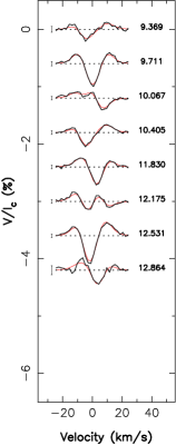
Figure 2: Stokes $V$ LSD profiles of DT Vir=GJ 494A (thick black line) along with the maximum entropy fit (thin red line) to the data, for both the 2007 (left) and 2008 (right) runs. The rotational cycle of each observation, along with 3$\sigma$ error bars, are shown next to each profile.

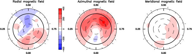
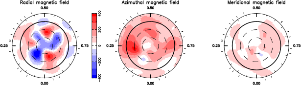
Figure 3: Magnetic topologies of DT Vir=GJ 494A in 2007 (top) and 2008 (bottom), reconstructed from a fit to the complete series of LSD Stokes $V$ profiles. The three components of the field in spherical coordinates are displayed (from left to right), with magnetic fluxes labelled in G. The star is shown in flattened polar projection down to latitudes of $-30\hbox{${}^{\circ}$}$, with the equator depicted as a bold circle and parallels as dashed circles. Radial ticks around each plot indicate the phases of observation.

As obvious from Fig. 3, the magnetic topologies we derive contain a significant amount of toroidal field (62% and 47% of the reconstructed magnetic energy in 2007 and 2008 respectively); at both epochs, the reconstructed toroidal field shows up as a ring of counterclockwise field encircling the whole star. The poloidal field is more complex, especially in 2008 when more than 50% of the reconstructed poloidal field energy concentrates in orders with $\ell>3$ (with dipole modes containing only 10%). The intrinsic evolution of the large-scale field topology between 2007 and 2008 is straightforwardly visible in the image, especially on the poloidal field component whose spatial structure was much simpler in 2007 (64% of the poloidal field energy in dipole modes). At both epochs, the reconstructed poloidal field is mostly non axisymmetric (less than 20% of the energy concentrating in $m<\ell/2$ modes). This information is summarised in Table 8.

5 DS Leo = GJ 410 = HD 95650 = HIP 53985

DS Leo is a single M0 dwarf with sharp spectral lines, located at an Hipparcos distance of $11.66\pm 0.18$ pc from the Sun. Its RV is equal to $-13.90\pm 0.10$ km s^-1 (Nidever et al., 2002). Photometric variability was studied by Fekel & Henry (2000) who detected cyclic variability at periods of 13.99 d and 15.71 d on different observing seasons and interpreted it as caused by stellar rotation (about 14 d) coupled to surface differential rotation (modulating the observed photometric period as spots migrate to different latitudes). Using the mass-luminosity relations of Delfosse et al. (2000), we estimate that the mass of DS Leo is $0.58\pm 0.02$ ${\rm M}_{\odot}$, i.e. very similar to that of DT Vir. The large amplitude rotational modulation that we observe for Stokes $V$ profiles suggest that the inclination angle is not small; we therefore set $i=60\hbox{${}^{\circ}$}$ in the following imaging process.

Stokes $V$ data were collected at 2 epochs (same runs as for DT Vir, see Table 3), providing again partial coverage of the rotation cycle at the first epoch but a dense and redundant coverage at the second epoch. Stokes $V$ signatures are detected in almost all spectra, with longitudinal fields never exceeding strengths of 35 G. The RV we measure ($-14.05\pm 0.10$ km s^-1 at both epochs, with an internal dispersion of 0.03 km s^-1) is in reasonbly good agreement with that of Nidever et al. (2002). The rotational broadening of DS Leo is small, only slightly larger than that of GJ 205 (having $\hbox{$v\sin i$}=1.0-1.5$ km s^-1, Reiners, 2007); using $\hbox{$v\sin i$}=2\pm 1$ km s^-1 provides a good fit to the Stokes $I$ profiles and is compatible with the radius expected from theoretical models (0.52 ${\rm R}_{\odot}$, see Table 1), the rotation period of Fekel & Henry (2000) and the inclination angle we assumed ($i=60\hbox{${}^{\circ}$}$). As for DT Vir, we do not need to use $f$ for modelling the profiles of DS Leo.

The solid-body-rotation period providing the best fit to the data is close to 14 d at both epochs; we therefore used it to phase all spectra. As for DT Vir, the $B_{\rm\ell}$ curve in the 2008 data is showing apparently discrepant points for spectra collected at nearby phases but different cycles (e.g., Jan 03 and Feb 14, at rotation cycles 26.336 and 29.328) as a likely result of the presence of surface differential rotation. This is confirmed by the fact that the full Stokes $V$ 2008 data set cannot be fitted down to $\hbox{$\chi^{2}_{\nu}$}=1$ when assuming solid body rotation. Proceeding as for DT Vir, we obtain that $\hbox{$\Omega_{\rm eq}$}=0.465\pm 0.004$ rad d^-1 and $\hbox{$d\Omega$}=0.076\pm 0.020$ rad d^-1 at the surface of DS Leo, i.e., that the rotation periods at the equator and the pole are respectively equal to 13.5 d and 16.1 d (bracketing both photometric periods of Fekel & Henry 2000). The photospheric shear of DS Leo is thus very similar to that of DT Vir, with the equator lapping the pole by one cycle every $83_{-20}^{+30}$ d.

The optimal maximum entropy fit to the Stokes $V$ data that we obtain (including the effect of differential rotation) is shown in Fig. 4 and corresponds to $\hbox{$\chi^{2}_{\nu}$}=0.9$, i.e., to a $\chi^{2}_{\nu}$ improvement over a non-magnetic model of $\times 15$ and $\times 8$ for each epoch respectively. The reconstructed magnetic maps are shown in Fig. 5.

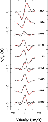
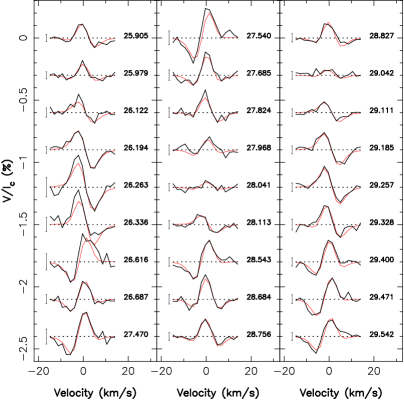
Figure 4: Same as Fig. 2 for DS Leo=GJ 410.

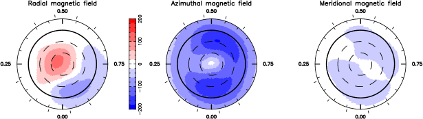
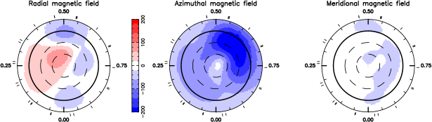
Figure 5: Same as Fig. 3 for DS Leo=GJ 410.

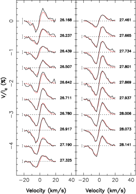
Figure 6: Same as Fig. 2 for CE Boo=GJ 569A.

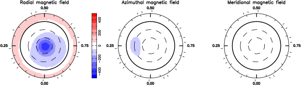
Figure 7: Same as Fig. 3 for CE Boo=GJ 569A.

The magnetic topologies we derive are predominantly toroidal (more than 80% of the reconstructed magnetic energy at both epochs), with the reconstructed toroidal field showing up as a ring of clockwise field encircling the star. The poloidal field is much simpler than that of DT Vir (partly because of the lower spatial resolution resulting from the smaller $v\sin i$) and consists mostly in a dipole (containing more than 50% of the poloidal field energy) evolving from a mainly axisymmetric to a mainly non-axisymmetric configuration between 2007 and 2008. Eventhough the fractional energy stored in the various field components remained grossly stable (see Table 8), the magnetic topology underwent significant temporal evolution between both epochs, e.g., with the toroidal field ring showing 2 extrema across the star in 2007 while it only shows one in 2008.

6 CE Boo = GJ 569A = HIP 72944

CE Boo is a young and active M2.5 dwarf with sharp spectral lines, located at an Hipparcos distance of $9.81\pm 0.16$ pc. It is the brightest member of a multiple (possibly quadruple) system with an estimated age of only $\simeq 100$ Myr (Simon et al., 2006). The companions are located about 5^′′ (i.e., 50 AU) away and consist of at least a brown dwarf binary and possibly even a triple. Using the mass-luminosity relations of Delfosse et al. (2000), we estimate a mass of $0.48\pm 0.02$ ${\rm M}_{\odot}$. The current RV is equal to $-7.21\pm 0.10$ (Nidever et al., 2002). From photometric variability, Kiraga & Stepien (2007) find that the rotation period is 13.7 d; this is surprisingly long for a star as young as CE Boo, even longer than the average period for M dwarfs of the young galactic disc (whose age is typically a few Gyr, Kiraga & Stepien 2007). The activity of CE Boo is slightly larger than that of DS Leo (but smaller than that of DT Vir, see Table 1), in agreement with what is expected for a star with a similar period and a later spectral type. The sharp lines of CE Boo also argue in favour of the slow rotation.

Stokes $V$ data were collected in early 2008 only, with a rather dense coverage of the rotation cycle (see Table 4); Stokes $V$ signatures are detected at all times, with longitudinal fields ranging from –50 G and –120 G and evolving smoothly with rotation phase. The RV we measure ($-7.34\pm 0.10$ km s^-1, with an internal dispersion of 0.03 km s^-1) agrees with that of Nidever et al. (2002). The rotational modulation of the Stokes $V$ profiles are reminiscent of those of AD Leo (M08), suggesting that the star is not seen equator on; the relative fluctuations of the longitudinal fields are however about twice larger than those of AD Leo, indicating that $i$ is not as low as 20^∘ (as for AD Leo). We chose $i=45\hbox{${}^{\circ}$}$ as a an intermediate value. The rotational broadening in the spectral lines of CE Boo is small, comparable to that of DS Leo; using the radius expected from theoretical models (0.43 ${\rm R}_{\odot}$, see Table 1), the rotation period of Kiraga & Stepien (2007) and the inclination angle we assumed ($i=45\hbox{${}^{\circ}$}$), we find (and used) $\hbox{$v\sin i$}=1$ km s^-1. Conversely to the 2 previous stars, we have to assume $f=0.05$ (smaller than the usual value for mid-M dwarfs, see M08) to obtain a $\hbox{$\chi^{2}_{\nu}$}=1$ to the Stokes $V$ profiles.

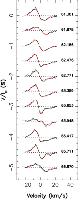
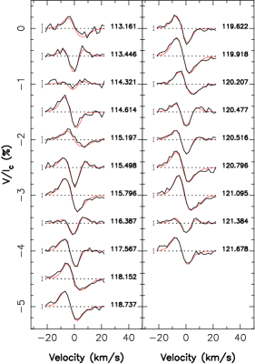
Figure 8: Same as Fig. 2 for OT Ser=GJ 9520.

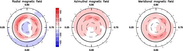
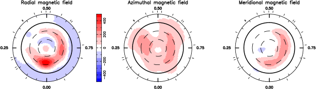
Figure 9: Same as Fig. 3 for OT Ser=GJ 9520.

The solid-body-rotation period providing the best fit to the Stokes $V$ data is equal to 14.7 d, which we used to phase all our spectra. This is slightly longer than the period found by Kiraga & Stepien (2007), suggesting that CE Boo is also subject to differential rotation (as DT Vir and DS Leo) with at least $\hbox{$d\Omega$}=0.03$ rad d^-1 (assuming our period yields the rotation rate at the pole and the period of Kiraga & Stepien 2007 traces the rotation rate at the equator). Proceeding as above, we obtain no clear minimum in the $\Omega_{\rm eq}$–$d\Omega$ domain, indicating that our data are not suitable for measuring differential rotation; this is not too surprising given the fairly simple rotational modulation of the Stokes $V$ profiles and its moderate amplitude. We therefore assumed that CE Boo rotates as a solid-body in the following; very similar results are obtained if assuming that CE Boo is hosting differential rotation similar to that of DT Vir and DS Leo.

The optimal maximum entropy fit to the Stokes $V$ data that we obtain is shown in Fig. 6 and corresponds to $\hbox{$\chi^{2}_{\nu}$}=1$, i.e., to a $\chi^{2}_{\nu}$ improvement over a non-magnetic model of $\times 35$. The reconstructed magnetic map is shown in Fig. 7. The magnetic topology we derive is almost completely poloidal, with less that 10% of the reconstructed energy concentrating into the toroidal component (see Table 8); the poloidal field is quite simple (93% of the energy in the $\ell\leq 2$ modes) and mostly axisymmetric (96% of the energy in $m<\ell/2$ modes).

7 OT Ser = GJ 9520 = HIP 75187

OT Ser is an active M1.5 dwarf with spectral lines showing significant rotational broadening. Located at an Hipparcos distance of $11.39\pm 0.25$ pc, it has no identified companion (Daemgen et al., 2007, Forveille private communication). Using the mass-luminosity relations of Delfosse et al. (2000), we estimate a mass of $0.55\pm 0.02$ ${\rm M}_{\odot}$. Two discrepant rotation periods, both estimated from photometric variability, are reported in the literature; while Norton et al. (2007) find $\hbox{$P_{\rm rot}$}=3.38$ d, Kiraga & Stepien (2007) obtain $\hbox{$P_{\rm rot}$}=0.37$ d. Given the estimated radius of OT Ser (about 0.5 ${\rm R}_{\odot}$, see Table 1), the second period would imply an equatorial velocity of almost 70 km s^-1, much larger than the observed width of spectral lines; the rotation period of Norton et al. (2007) is thus much more likely to be the correct one.

Stokes $V$ data were collected in 2007 and 2008, with a rather dense coverage of the rotation cycle in 2008 (see Table 5); Stokes $V$ signatures are detected in almost all spectra. The longitudinal field variations with phase are very different at both epochs (with $B_{\rm\ell}$ varying from 55 to 80 G in 2007 and from –10 to 110 G in 2008) demonstrating that the magnetic topology changed significantly on a timescale of only 0.5 yr. The RV we measure ($6.77\pm 0.10$ km s^-1 and $6.83\pm 0.10$ km s^-1, with internal dispersions of 0.03 km s^-1and 0.04 km s^-1) are slightly different at both epochs, possibly reflecting the change in the magnetic topology. Modelling Stokes $I$ line profiles yields $\hbox{$v\sin i$}=6\pm 1$ km s^-1. From the expected radius and rotation period, we infer that the star is seen at an intermediate inclination angle; we use $i=45\hbox{${}^{\circ}$}$ in the following. As for CE Boo, we have to adjust $f$ to obtain a $\hbox{$\chi^{2}_{\nu}$}=1$ fit to the Stokes $V$ profiles; we find that $f$ equals 0.05 and 0.10 in 2007 and 2008 respectively.

The solid-body-rotation period providing the best fit to the data is equal to 3.40 d at both epochs; we used it to phase all our data (see Table 5). This period is close to but slightly different than that of Norton et al. (2007), suggesting that OT Ser is also differentially rotating. Fitting our 2008 Stokes $V$ data further confirms that OT Ser is not rotating as a solid body; with the same procedure as above, we obtain that $\hbox{$\Omega_{\rm eq}$}=1.88\pm 0.01$ rad d^-1 and $\hbox{$d\Omega$}=0.12\pm 0.02$ rad d^-1, i.e., that the rotation periods at the equator and the pole are respectively equal to 3.34 d and 3.57 d. The photospheric shear of OT Ser is thus apparently even stronger than that of DT Vir and DS Leo, with the equator lapping the pole by one cycle every $52_{-7}^{+11}$ d.

The optimal maximum entropy fit to the Stokes $V$ data that we obtain (including the effect of differential rotation) is shown in Fig. 8 and corresponds to $\hbox{$\chi^{2}_{\nu}$}=1$, i.e., to a $\chi^{2}_{\nu}$ improvement over a non-magnetic model of $\times 23$ and $\times 19$ for 2007 and 2008 respectively. The reconstructed magnetic maps are shown in Fig. 9. Although both maps show a similar large-scale topology (e.g., same latitudinal dependence of field polarities for all components), differences are nevertheless obvious; for instance, the ring of positive radial field encircling the star at mid latitudes shows a prominent blob at phase 0.0 in 2008 (causing the large-amplitude longitudinal-field modulation observed at this epoch).

The magnetic topologies we derive are dominantly poloidal, with about 20–30% of the reconstructed energy concentrating into the toroidal component; the poloidal field is mostly axisymmetric and includes a significant dipole component at both epochs (see Table 8).

8 GJ 182 = HIP 23200

GJ 182 is a very young single M0.5 dwarf of the IC 2391 supercluster located at an Hipparcos distance of $26.7\pm 1.7$ pc. The star is surrounded by a massive debris disk indicating on-going planetary formation (Liu et al., 2004), further demonstrating that it is indeed very young. Its position in the HR diagram (about 0.5 mag above the main sequence) is in agreement with the age of its young moving group (about 35 Myr, e.g., Montes et al. 2001). Using the evolutionary models of Baraffe et al. (1998) and matching them to an absolute $V$ magnitude and a logarithmic luminosity (relative to the Sun) of $7.94$ and $-0.83$ respectively, we find that GJ 182 has a mass of $0.75$ ${\rm M}_{\odot}$, a radius of $0.82$ $R_{\star}$, a temperature of 3950 K and an age of 25 Myr; this is what we assume in the following. The high lithium content of GJ 182 suggests that the star is even younger, possibly as young as 10–15 Myr (Favata et al., 1998) as evolutionary models predict that lithium should be already strongly depleted at 20 Myr (Favata et al., 1998). Effects of rotation and magnetic fields on the stellar structure and on the evolution (e.g., Chabrier et al., 2007, not taken into account in existing studies) are however likely to affect model predictions significantly.

Stokes $V$ data were collected in 2007, covering only about half the rotation cycle of GJ 182 (see Table 6); Stokes $V$ signatures are detected in all spectra and longitudinal field vary from –90 G to 20 G with rotation phase. The RV we measure ($19.35\pm 0.10$ km s^-1, with an internal dispersion of 0.18 km s^-1) varies with rotational phase and correlate well with longitudinal field values; although the statistics is moderately significant (only 7 data points available), it suggests that the RV fluctuations we detect (full amplitude of about 0.4 km s^-1) are related to surface magnetic activity. Spectral lines are significantly broadened by rotation; modelling Stokes $I$ LSD profiles yield $\hbox{$v\sin i$}=10\pm 1$ km s^-1. Photometric modulation indicates a rotation period of about 4.4 d (Kiraga & Stepien, 2007), suggesting that the star is viewed equator-on rather than pole-on; we therefore set the inclination angle at $i=60\hbox{${}^{\circ}$}$.

The solid-body-rotation period providing the best fit to the data is equal to 4.35 d, slightly smaller than the photometric period of 4.41 d measured by Kiraga & Stepien (2007); we used our estimate to phase all spectra, and take this as a likely indication that GJ 182 is a differential rotator. Despite the small number of spectra and the limited phase coverage, fitting our Stokes $V$ data down to $\hbox{$\chi^{2}_{\nu}$}=1$ suggests that GJ 182 is indeed not rotating as a solid body. Using the procedure described in Sec. 3, we obtain that $\hbox{$\Omega_{\rm eq}$}=1.46\pm 0.01$ rad d^-1 and $\hbox{$d\Omega$}=0.06\pm 0.03$ rad d^-1; the corresponding rotation periods at the equator and the pole are respectively equal to 4.30 d and 4.49 d (bracketing both our rotation period and that of Kiraga & Stepien 2007). Solid-body rotation is excluded at the 2$\sigma$ level; more data are needed to confirm this with better precision.

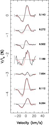
Figure 10: Same as Fig. 2 for GJ 182.

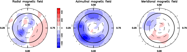
Figure 11: Same as Fig. 3 for GJ 182.

The optimal maximum entropy fit to the Stokes $V$ data that we obtain (including the effect of differential rotation) is shown in Fig. 10 and corresponds to $\hbox{$\chi^{2}_{\nu}$}=1$, i.e., to a $\chi^{2}_{\nu}$ improvement over a non-magnetic model of $\times 22$. The reconstructed magnetic map is shown in Fig. 11. The magnetic field is dominantly toroidal, and the poloidal component is mostly non-axisymmetric (see Table 8).

9 GJ 49 = HIP 4872

GJ 49 is a single M1.5 dwarf with sharp spectral lines and relatively low activity; it is the least active star of our sample (see Table 1). The Hipparcos distance is equal to $10.06\pm 0.14$ pc. No rotation periods are found in the literature; the RV is reported to be $-5.97\pm 0.10$ (Nidever et al., 2002). Using the mass-luminosity relations of Delfosse et al. (2000), we estimate a mass of $0.57\pm 0.02$ ${\rm M}_{\odot}$.

Stokes $V$ data were collected in 2007, covering the whole rotation cycle of GJ 49 (see Table 7); Stokes $V$ signatures are detected in all spectra, with longitudinal fields ranging from –30 G to 0 G across the cycle. The RV we measure ($-6.02\pm 0.10$ km s^-1, with an internal dispersion of 0.02 km s^-1) is in good agreement with that of Nidever et al. (2002). Modelling Stokes $I$ LSD profiles indicates that the rotational broadening is very small; we thus set $\hbox{$v\sin i$}=1$ km s^-1.

We determine the rotation period by selecting the one with which the Stokes $V$ profiles can be fitted at $\hbox{$\chi^{2}_{\nu}$}=1$ with smallest magnetic energy in the reconstructed image; we find that $\hbox{$P_{\rm rot}$}=18.6\pm 0.3$ d; we also find that an intermediate inclination angle ($i\simeq 45\hbox{${}^{\circ}$}$) minimises the amount of reconstructed magnetic information. We find that the data are compatible with solid-body rotation, but the accuracy to which we measure $d\Omega$ (error bar $\simeq 0.05$ rad d^-1) is not high enough to know whether GJ 49 also hosts differential rotation similar to that found on the other sample stars.

The fit to the Stokes $V$ data that we obtain is shown in Fig. 12 and corresponds to a $\chi^{2}_{\nu}$ improvement over a non-magnetic model of $\times 11$. The reconstructed magnetic map is shown in Fig. 13. The poloidal and toroidal field components roughly share the same amount of energy, with the poloidal field being mainly dipolar and axisymmetric (see Table 8).

10 Summary and discussion

We report in this paper the results of our spectroscopic survey of M dwarfs; following M08 (concentrating on mid-M dwarfs), we describe here the Zeeman signatures and the large-scale magnetic topologies we observed on 6 early-M dwarfs (from M0 to M3). We also determined or confirmed the rotation period of all stars (ranging from 2.8 to 18.6 d), and detected significant surface differential rotation in 4 of them (with a strength comparable to that of the Sun).

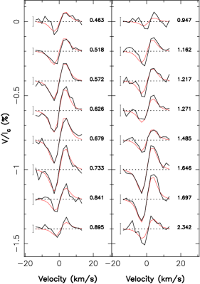
Figure 12: Same as Fig. 2 for GJ 49.

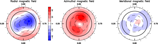
Figure 13: Same as Fig. 3 for GJ 49.

The magnetic fields we detect in early-M dwarfs are weak (typically a few tens of G), smaller in particular than those found in mid-M dwarfs (M08) by typically a factor of 5 (see Fig. 14) with a sharp transition occuring at 0.4 ${\rm M}_{\odot}$ (see Fig. 15, left panel). The large-scale magnetic topologies we derive are also significantly different, involving a much larger fraction of toroidal fields and a lower axisymmetric degree of poloidal fields whenever $\hbox{$M_{\star}$}>0.5$ ${\rm M}_{\odot}$ (5 stars in the present sample); below 0.5 ${\rm M}_{\odot}$, the poloidal field is largely dominant and axisymmetric and its strength is increasing rapidly as mass decreases. We also observe that the typical lifetime of the large-scale magnetic topology is very different on both sides of the 0.4–0.5 ${\rm M}_{\odot}$ threshold, with lifetimes smaller than a few months on the hot side and longer than 1 yr on the cool side (M08). This threshold is very sharp and well defined, with little apparent dependence with the rotation period.

At this stage, it is interesting to consider the effective Rossby number $Ro$, defined as $Ro=\hbox{$P_{\rm rot}$}/\tau_{\rm c}$ where $\tau_{\rm c}$ is the convective turnover time; in particular, $Ro$ is a convenient parameter for comparing the strength of dynamo action (and, e.g., $\log R_{\rm X}$ that indirectly reflects dynamo action through coronal heating) in stars with different masses. Figure 15 (right panel) illustrates how $\log R_{\rm X}$ smoothly varies with $Ro$ for both early- and mid-M dwarfs studied here and in M08; we find that $\log R_{\rm X}$ increases steeply with decreasing $Ro$ until $Ro\simeq 0.1$ where $\log R_{\rm X}$ saturates at a level of about –3.0, in good agreement with previous studies (e.g., James et al., 2000). Only GJ 182 (at $Ro=0.17$) lies slightly above the overall trend, as a likely consequence of its extreme youth and the related differences in its internal structure.

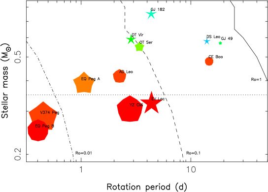
Figure 14: Basic properties of the large-scale magnetic properties of early- and mid-M dwarfs as a function of stellar mass and rotation period. Symbols size indicates magnetic energies, symbol colour illustrates the field configuration (blue and red for purely toroidal and purely poloidal fields respectively) while symbol shape depicts the degree of axisymmetry of the poloidal field component (decagon and stars for a purely axisymmetric and purely non-axisymmetric poloidal fields respectively). Results for early-M stars are from this paper and results for mid-M stars are from M08. The full, dashed and dash-dot lines respectively trace the location of the $Ro=1$, 0.1 and 0.01 contours, while the dotted line shows the theoretical full-convection threshold ($\hbox{$M_{\star}$}\simeq 0.35$ ${\rm M}_{\odot}$).

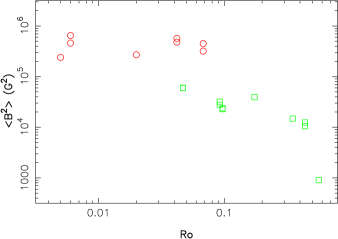
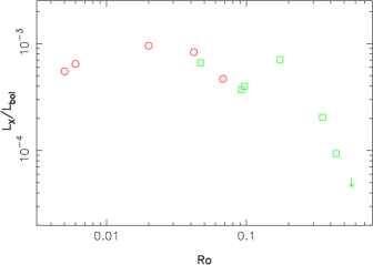
Figure 15: Reconstructed magnetic energy (left) and relative X-ray luminosity (with respect to the bolometric luminosity, right) as a function of $Ro$ for stars studied in this paper and in M08. Stars with masses larger and smaller than 0.4 ${\rm M}_{\odot}$ are shown as green squares and red circles respectively. In the left panel, measurements at different epochs (whenever available) are shown for each star to illustrate the typical scatter expected from temporal variability.

We note that the abrupt step in the large-scale magnetic energy between early- and mid-M dwarfs (see Fig. 15, left panel) apparently correlates better with stellar mass than with $Ro$; at $Ro=0.05$, AD Leo exhibits a magnetic flux compatible with that of all other early M dwarfs, but significantly weaker than that of EV Lac (at $Ro=0.07$) and YZ CMi (at $Ro=0.04$). More data are needed to confirm this point, especially for high-mass rapid rotators (i.e., having $Ro\simeq 0.01$ and $\hbox{$M_{\star}$}>0.5$ ${\rm M}_{\odot}$) and low-mass slow rotators (with $Ro>0.1$ and $\hbox{$M_{\star}$}<0.4$ ${\rm M}_{\odot}$). We also note that this abrupt step does not show up in the $\log R_{\rm X}$ vs $Ro$ plot of Fig. 15 (right panel); this is presumably because X-rays are sensitive to overall magnetic energies while we are only sensitive to the largest scales. Our result therefore suggests that, at some specific stellar mass ($\simeq 0.4$ ${\rm M}_{\odot}$, rather than at some specific $Ro$), dynamo processes become suddenly much more efficient at triggering large-scale magnetic fields; we also observe that, at more or less the same mass ($\simeq 0.5$ ${\rm M}_{\odot}$), large-scale topologies of M dwarfs become dominantly poloidal and axisymmetric. Note however that, even in the case of mid-M dwarfs, the large-scale fields we derive are significantly smaller than the corresponding equipartition field (a few kG, M08).

Table 8: Properties of the large-scale field topologies derived in the present study. For each star, observations at different epochs are listed separately. The table lists sequentially the name of the star, the mass, the rotation period, the effective Rossby number and the logarithmic relative X-ray luminosity (taken from Table 1), the surface angular rotation shear between the equator and pole $d\Omega$ (whenever detected), the derived filling factor $f$ (whenever applicable), the reconstructed magnetic energy and flux (i.e., $<B^{2}>$ and $<B>$), and the fractional energies in the poloidal field, the poloidal dipole ($\ell=1$) modes, the poloidal quadrupole ($\ell=2$) modes, the poloidal octupole ($\ell=3$) modes, and the poloidal axisymmetric ($m<\ell/2$) modes. All field components with $\ell\leq 3$ are required to fit the data at noise level.

Star	$M_{\star}$	$P_{\rm rot}$	$Ro$	$\log R_{\rm X}$	$d\Omega$	$f$	$<B^{2}>$	$<B>$	pol	dip	qua	oct	axi
	(${\rm M}_{\odot}$)	(d)			(rad d-1)		($10^{4}$ G2)	(G)
GJ 182 2007	0.75	4.35	0.174	–3.1	$0.06\pm 0.03$		3.95	172	0.32	0.48	0.18	0.14	0.17
DT Vir 2007	0.59	2.85	0.092	–3.4			2.78	145	0.38	0.64	0.17	0.08	0.12
2008					$0.060\pm 0.006$		3.21	149	0.53	0.10	0.17	0.17	0.20
DS Leo 2007	0.58	14.0	0.438	–4.0			1.24	101	0.18	0.52	0.37	0.08	0.58
2008					$0.076\pm 0.020$		1.05	87	0.20	0.52	0.31	0.07	0.16
GJ 49 2007	0.57	18.6	0.564	$<-4.3$			0.09	27	0.48	0.71	0.20	0.07	0.67
OT Ser 2007	0.55	3.40	0.097	–3.4		0.05	2.28	136	0.80	0.47	0.19	0.18	0.86
2008					$0.12\pm 0.02$	0.10	2.38	123	0.67	0.33	0.17	0.21	0.66
CE Boo 2008	0.48	14.7	0.350	–3.7		0.05	1.48	103	0.95	0.87	0.06	0.03	0.96

Significant surface toroidal fields are detected even in DS Leo and GJ 49, i.e., the two slowest rotators with masses larger than 0.5 ${\rm M}_{\odot}$; it suggests that the transition between mainly poloidal and mainly toroidal fields in $\hbox{$M_{\star}$}>0.5$ ${\rm M}_{\odot}$ stars occurs at $Ro\simeq 0.5-1.0$, with the Sun located on the other side of this boundary (at $Ro\simeq 1.5-2.0$). Note that this boundary coincides with the sharp onset of photometric variability in convective stars (occuring below $Ro\simeq 0.7$, Hall 1991). With a poloidal field concentrating 70–80% of the reconstructed magnetic energy, OT Ser is off this trend; we suspect that this is due to its proximity with the 0.5 ${\rm M}_{\odot}$ sharp threshold below which magnetic topologies become dominantly poloidal.

Early-M dwarfs are found to show significant differential rotation; the values we obtain for the surface angular rotation shear $d\Omega$ ranges from 0.06 to 0.12 rad d^-1, i.e., from once to twice the strength of the surface latitudinal shear of the Sun. Our detection is further confirmed by the small (but significant) differences between the rotation periods we measure and the values reported in the literature (derived from photometric fluctuations) and by the short lifetimes of the large-scale field topologies (quickly distorted beyond recognition by differential rotation). Previous Doppler imaging studies of early-M dwarfs with very fast rotation ($Ro\simeq 0.01$) report that differential rotation is very small (Barnes et al., 2005); our study suggests that the situation may significantly differ in moderate rotators like those we considered. Our result is also different from what is observed in mid-M dwarfs where differential rotation is very small (a few mrad d^-1 at most, i.e., more than 10 times smaller than that of early-M dwarfs, M08) and large-scale magnetic topologies long-lived (M08). It is not clear yet what this difference is due to; while small $Ro$ may contribute at freezing differential rotation, this is likely not the only relevant parameter for this problem (e.g., with DT Vir and EV Lac showing respectively significant and no differential rotation despite their similar $Ro$).

The sharp transition that we report between the magnetic (and differential rotation) properties of early- and mid-M dwarfs is surprising at first glance; naively, one would expect the properties of large-scale magnetic fields to change smoothly with stellar mass as the radiative core gets progressively smaller. From the evolutionary models of Siess et al. (2000), we however note that the outer radius of the radiative core of early-M dwarfs is changing very quickly with stellar mass, from about 0.5 $R_{\star}$ for a 0.5 ${\rm M}_{\odot}$ star to a negligible fraction for a 0.4 ${\rm M}_{\odot}$ star. We speculate that this sharp transition is the main reason for the abrupt magnetic threshold that we report here. The rapid increase in empirical convective turnover times occuring at about the same location (Kiraga & Stepien, 2007) also likely contributes at making the transition between both dynamo regimes very sharp.

The most recent dynamo simulations of fully convective M dwarfs (Browning, 2008) (carried out for $Ro\simeq 0.01$) are successful at reproducing the frozen differential rotation that we observe (M08); they however predict the presence of strong toroidal fields that we do not see in mid-M dwarfs with similar $Ro$. We speculate that the abrupt change in the large-scale magnetic topology of M dwarfs that we report here to occur at spectral type M3 may also be (at least partly) responsible for the reduced magnetic braking observed for stars later than M3 (e.g., Delfosse et al., 1998); MHD simulations of magnetic winds are necessary to estimate quantitatively whether the observed change in the large-scale magnetic topology can indeed explain the longer spin-down timescales.

In the two stars having $v\sin i$ measured with sufficient precision (i.e., $\hbox{$v\sin i$}\geq 10$, GJ 182 and DT Vir), we find that $\hbox{$R_{\star}$}\sin i$ (equal to $0.86\pm 0.09$ ${\rm R}_{\odot}$ and $0.62\pm 0.06$ ${\rm R}_{\odot}$ respectively) is already larger than the predicted radius from theoretical models (Baraffe et al., 1998); while this could result from overestimating the true age (and hence underestimating the true radius) of GJ 182, this explanation does not apply for DT Vir, for which we conclude that the observed radius is truly larger (by at least 10% and potentially as much as 30%) that what theoretical models predict. A similar conclusion is reached for V374 Peg (Donati et al., 2006a; Morin et al., 2008a); furthermore, M08 obtains that $\hbox{$R_{\star}$}\sin i$ is equal to the predicted theoretical radius (within the error bars) for 4 other active stars, suggesting again that $R_{\star}$ is larger than expected. Following Chabrier et al. (2007), we propose that this effect is a direct consequence of magnetic fields getting strong enough (and hence saturating the dynamo, see Fig. 15) to affect the energy transport throughout the convective zone and hence the radius. Our results therefore independently confirm the report that cool low-mass active stars, either single (Morales et al., 2008) or within close eclipsing binaries (Ribas, 2006), usually have oversized radii with respect to inactive stars of similar spectral types.

We also detect significant RV fluctuations (with a full amplitude of up to 0.40 km s^-1) in the 3 very active stars of our sample (with rotation periods smaller than 5 d). For the most active ones (DT Vir and GJ 182, showing the largest RV modulation), the RV variations correlate reasonably well (though not perfectly) with longitudinal fields, suggesting that the origin of the variations is indeed the magnetic field (and the underlying activity). It also suggests that spectropolarimetric observations should be carried out simultaneously with RV measurements of active stars to enable filtering out efficiently the activity jitter from the RV signal; this technique may prove especially useful when looking at Earth-like habitable planets orbiting around M dwarfs in the future, e.g., with a nIR spectropolarimeter such as SPIRou (a nIR counterpart of ESPaDOnS, proposed for CFHT).

Our spectropolarimetric survey is an on-going study; we are now concentrating on late-M dwarfs (M5-M8) to derive similar observational constraints about the large-scale magnetic topologies of stars in the yet unexplored 0.08–0.20 ${\rm M}_{\odot}$ region of Fig. 14 to investigate how dynamo processes operate down to the brown dwarf threshold, i.e., when stellar atmospheres get so cool that they start to decouple from their magnetic fields.

References

- Baraffe et al. (1998) Baraffe I., Chabrier G., Allard F., Hauschildt P. H., 1998, A&A, 337, 403
- Barnes et al. (2005) Barnes J. R., Cameron A. C., Donati J.-F., James D. J., Marsden S. C., Petit P., 2005, MNRAS, 357
- Beuzit et al. (2004) Beuzit J.-L., Ségransan D., Forveille T., Udry S., Delfosse X., Mayor M., Perrier C., Hainaut M.-C., Roddier C., Roddier F., Martín E. L., 2004, A&A, 425, 997
- Browning (2008) Browning M. K., 2008, ApJ, 676, 1262
- Chabrier et al. (2007) Chabrier G., Gallardo J., Baraffe I., 2007, A&A, 472, L17
- Charbonneau (2005) Charbonneau P., 2005, Living Reviews in Solar Physics, 2, 2
- Daemgen et al. (2007) Daemgen S., Siegler N., Reid I. N., Close L. M., 2007, ApJ, 654, 558
- Delfosse et al. (1998) Delfosse X., Forveille T., Perrier C., Mayor M., 1998, A&A, 331, 581
- Delfosse et al. (2000) Delfosse X., Forveille T., Ségransan D., Beuzit J.-L., Udry S., Perrier C., Mayor M., 2000, A&A, 364, 217
- Dobler et al. (2006) Dobler W., Stix M., Brandenburg A., 2006, ApJ, 638, 336
- Donati (2003) Donati J.-F., 2003, in Trujillo-Bueno J., Sanchez Almeida J., eds, Astronomical Society of the Pacific Conference Series Vol. 307 of Astronomical Society of the Pacific Conference Series, ESPaDOnS: An Echelle SpectroPolarimetric Device for the Observation of Stars at CFHT. pp 41–+
- Donati et al. (2003a) Donati J.-F., Cameron A., Semel M., Hussain G., Petit P., Carter B., Marsden S., Mengel M., Lopez Ariste A., Jeffers S., Rees D., 2003a, MNRAS, 345, 1145
- Donati et al. (2003b) Donati J.-F., Collier Cameron A., Petit P., 2003b, MNRAS, 345, 1187
- Donati et al. (2006a) Donati J.-F., Forveille T., Cameron A. C., Barnes J. R., Delfosse X., Jardine M. M., Valenti J. A., 2006a, Science, 311, 633
- Donati et al. (2006b) Donati J.-F., Howarth I. D., Jardine M. M., Petit P., Catala C., Landstreet J. D., Bouret J.-C., Alecian E., Barnes J. R., Forveille T., Paletou F., Manset N., 2006b, MNRAS, 370, 629
- Donati et al. (2008) Donati J.-F., Jardine M. M., Gregory S. G., Petit P., Paletou F., Bouvier J., Dougados C., Ménard F., Cameron A. C., Harries T. J., Hussain G. A. J., Unruh Y., Morin J., Marsden S. C., Manset N., Aurière M., Catala C., Alecian E., 2008, MNRAS, 386, 1234
- Donati et al. (1997) Donati J.-F., Semel M., Carter B. D., Rees D. E., Cameron A. C., 1997, MNRAS, 291, 658
- Durney et al. (1993) Durney B. R., De Young D. S., Roxburgh I. W., 1993, Solar Physics, 145, 207
- Favata et al. (1998) Favata F., Micela G., Sciortino S., D’Antona F., 1998, A&A, 335, 218
- Fekel & Henry (2000) Fekel F. C., Henry G. W., 2000, AJ, 120, 3265
- Hall (1991) Hall D. S., 1991, in Tuominen I., Moss D., Rüdiger G., eds, IAU Colloq. 130: The Sun and Cool Stars. Activity, Magnetism, Dynamos Vol. 380 of Lecture Notes in Physics, Berlin Springer Verlag, Learning about stellar dynamos from long-term photometry of starspots. pp 353–+
- Heintz (1994) Heintz W. D., 1994, AJ, 108, 2338
- James et al. (2000) James D. J., Jardine M. M., Jeffries R. D., Randich S., Collier Cameron A., Ferreira M., 2000, MNRAS, 318, 1217
- Johns-Krull & Valenti (1996) Johns-Krull C. M., Valenti J. A., 1996, ApJ, 459, L95+
- Kiraga & Stepien (2007) Kiraga M., Stepien K., 2007, Acta Astronomica, 57, 149
- Kurucz (1993) Kurucz R., 1993, CDROM # 13 (ATLAS9 atmospheric models) and # 18 (ATLAS9 and SYNTHE routines, spectral line database). Smithsonian Astrophysical Observatory, Washington D.C.
- Landi degl’Innocenti (1992) Landi degl’Innocenti E., 1992, Magnetic field measurements. Solar Observations: Techniques and Interpretation, pp 71–+
- Liu et al. (2004) Liu M. C., Matthews B. C., Williams J. P., Kalas P. G., 2004, ApJ, 608, 526
- Montes et al. (2001) Montes D., López-Santiago J., Gálvez M. C., Fernández-Figueroa M. J., De Castro E., Cornide M., 2001, MNRAS, 328, 45
- Morales et al. (2008) Morales J. C., Ribas I., Jordi C., 2008, A&A, 478, 507
- Morin et al. (2008a) Morin J., Donati J.-F., Forveille T., Delfosse X., Dobler W., Petit P., Jardine M. M., Cameron A. C., Albert L., Manset N., Dintrans B., Chabrier G., Valenti J. A., 2008a, MNRAS, 384, 77
- Morin et al. (2008b) Morin J., Donati J.-F., Petit P., Forveille T., Delfosse X., Albert L., Aurière M., Cabanac R., Dintrans B., Farès R., Gastine T., Lignières F., Paletou F., Ramirez Velez J., Théado S., 2008b, MNRAS, submitted
- Moutou et al. (2007) Moutou C., Donati J.-F., Savalle R., Hussain G., Alecian E., Bouchy F., Catala C., Collier Cameron A., Udry S., Vidal-Madjar A., 2007, A&A, 473, 651
- Nidever et al. (2002) Nidever D. L., Marcy G. W., Butler R. P., Fischer D. A., Vogt S. S., 2002, ApJS, 141, 503
- Norton et al. (2007) Norton A. J., Wheatley P. J., West R. G., Haswell C. A., Street R. A., Collier Cameron A., Christian D. J., Clarkson W. I., Enoch B., Gallaway M., Hellier C., Horne K., Irwin J., Kane S. R., Lister T. A., Nicholas J. P., 2007, A&A, 467, 785
- Parker (1955) Parker E. N., 1955, ApJ, 122, 293
- Reiners (2007) Reiners A., 2007, A&A, 467, 259
- Ribas (2006) Ribas I., 2006, Ap&SS, 304, 89
- Saar & Linsky (1985) Saar S. H., Linsky J. L., 1985, ApJ, 299, L47
- Schmitt & Liefke (2004) Schmitt J. H. M. M., Liefke C., 2004, A&A, 417, 651
- Siess et al. (2000) Siess L., Dufour E., Forestini M., 2000, A&A, 358, 593
- Simon et al. (2006) Simon M., Bender C., Prato L., 2006, ApJ, 644, 1183
- Wood et al. (1994) Wood B. E., Brown A., Linsky J. L., Kellett B. J., Bromage G. E., Hodgkin S. T., Pye J. P., 1994, ApJS, 93, 287