A large stellar evolution database for population synthesis studies. IV. Integrated properties and spectra.

Abstract

This paper is the 4th in a series describing the latest additions to the BaSTI stellar evolution database, which consists of a large set of homogeneous models and tools for population synthesis studies, covering ages between 30 Myr and $\sim$20 Gyr and 11 values of $Z$ (total metallicity). Here we present a new set of low and high resolution synthetic spectra based on the BaSTI stellar models, covering a large range of simple stellar populations (SSPs) for both scaled solar and $\alpha$-enhanced metal mixtures. This enables a completely consistent study of the photometric and spectroscopic properties of both resolved and unresolved stellar populations, and allows us to make detailed tests on specific factors which can affect their integrated properties. Our low resolution spectra are suitable for deriving broadband magnitudes and colors in any photometric system. These spectra cover the full wavelength range (9–160000nm) and include all evolutionary stages up to the end of AGB evolution. Our high resolution spectra are suitable for studying the behaviour of line indices and we have tested them against a large sample of Galactic globular clusters. We find that the range of ages, iron abundances [Fe/H], and degree of $\alpha$-enhancement predicted by the models matches the observed values very well. We have also tested the global consistency of the BaSTI models by making detailed comparisons between ages and metallicities derived from isochrone fitting to observed colour-magnitude diagrams, and from line index strengths, for the Galactic globular cluster 47 Tuc and the open cluster M67. For 47 Tuc we find reasonable agreement between the 2 methods, within the estimated errors. From the comparison with M67 we find non-negligible effects on derived line indices caused by statistical fluctuations, which are a result of the specific method used to populate an isochrone and assign appropriate spectra to individual stars.

1 Introduction

Large grids of stellar models and isochrones are necessary tools to interpret photometric and spectroscopic observations of resolved and unresolved stellar populations. This, in turn, allows one to both test the theory of stellar evolution, and investigate the formation and evolution of galaxies, one of the major open problems of modern astrophysics.

To this purpose, we started in 2004 a major project aimed at creating a large and homogeneous database of stellar evolution models and isochrones (BaSTI – a Bag of Stellar Tracks and Isochrones) that cover a large chemical composition range relevant to stellar populations in galaxies of various morphological types. In addition, BaSTI includes the option of choosing between different treatments of core convection and stellar mass loss employed in the model calculations. In its present form, BaSTI contains a grid of models that cover stellar populations with ages ranging between 30 Myr and $\sim$20 Gyr, which include all evolutionary phases from the Main Sequence (MS) to the end of the Asymptotic Giant Branch (AGB) evolution or carbon ignition, depending on the value of stellar mass. They are calculated for two metal mixtures (scaled solar and $\alpha$-enhanced) and 11 values of $Z$ (total metallicity), each with two choices for the Reimers mass loss parameter $\eta$ (Reimers, 1975), and two mixing prescriptions during the Main Sequence (without and with overshooting from the Schwarzschild boundary). Broadband magnitudes and colors for the BaSTI models and isochrones are provided in various photometric systems (Johnson-Cousins, Sloan, Strömgren, Walraven, ACS/$HST$), making use of bolometric corrections derived from an updated set of model atmosphere calculations, for element mixtures consistent with those employed in the stellar evolution computations.

In addition to stellar models and isochrones, BaSTI also provides a series of Web tools that enable an interactive access to the database and make it possible to compute user-specified evolutionary tracks, isochrones, stellar luminosity functions (star counts in a stellar population as a function of magnitude) plus synthetic color-magnitude diagrams (CMDs) for arbitrary star formation histories (SFHs). The results of this major effort have been published in Pietrinferni et al. (2004, 2006, hereinafter Papers I and II) and Cordier et al. (2007, hereinafter Paper III). All Web tools, models and isochrones can be found at the BaSTI official website http://193.204.1.62/index.html.

The database has been extensively tested against observations of local stellar populations and eclipsing binary systems (see, for some examples, the tests presented in Papers I,  II and  III; Salaris et al. 2007; Tomasella et al. 2008). In its present form BaSTI can be used to investigate resolved stellar populations, and indeed it has been widely employed in studies of Galactic and extragalactic resolved star clusters (see, e.g. De Angeli et al., 2005; Villanova et al., 2007; Mackey & Broby Nielsen, 2007, for just a few examples) and in the determination of SFH and chemical enrichment history of resolved Local Group galaxies (see, e.g. Gallart et al., 2004; Barker et al., 2007; Gullieuszik et al., 2007; Carrera et al., 2008).

Integrated colors and magnitudes for simple (single-age, single metallicity) stellar populations (SSPs) can be easily determined from the isochrones. The only additional pieces of information needed are an Initial Mass Function (IMF) and the relationship between the initial and final (remnant) stellar masses. Indeed, some integrated colors from BaSTI models have already been tested against empirical constraints in Papers II and III. Moreover, James et al. (2006) and Salaris & Cassisi (2007) have already employed integrated colors from BaSTI isochrones to address issues related to the SFH of unresolved dwarf and elliptical galaxies, and extragalactic globular cluster ages.

A further development of BaSTI, which we present in this paper, is the inclusion of integrated spectra (including spectral line indices) for SSPs spanning the same parameter space – in terms of ages, metallicities and heavy element mixtures – covered by the isochrones of Papers I and II. Corresponding quantities for composite stellar populations with an arbitrary SFH can then be easily determined by integration over a range of discrete SSPs.

We present both low and high resolution versions suited to different purposes. Our low resolution spectra cover all evolutionary stages and are based on libraries of (predominantly) theoretical stellar spectra, consistent with those used to produce the bolometric corrections employed in the isochrone calculations. This ensures that our SSP integrated broadband magnitudes and colors obtained from either adding up the broadband fluxes of the individual stars populating the appropriate isochrone, or from their composite integrated spectrum, will be exactly the same (see test in section 2.1). Our high resolution spectra are suitable for deriving line strengths and making detailed tests of their behaviour as a function of age and chemical composition, and also horizontal branch morphology and sampling in the case of resolved stellar clusters (see tests in sections 3.1 and 3.2).

With the inclusion of predictions of both photometric and spectroscopic integrated properties of SSPs, BaSTI will provide a well tested, fully homogeneous and up-to-date set of theoretical tools that enable us to investigate self-consistently both resolved and unresolved stellar populations. We present a global test of this self-consistency and reliability of the database, by considering both the observed CMD and integrated spectrum of the well-studied clusters 47 Tuc and M67, to intercompare ages and metallicities obtained from our high-resolution spectra with the results from fitting theoretical isochrones to the observed CMD, and with independent chemical composition estimates from spectroscopy of individual stars.

The structure of the paper is as follows. A description of the method used to create our theoretical integrated spectra is given in Section 2, including separate detailed descriptions of our low and high resolution spectra in Sections 2.1 and 2.2 respectively. This is followed in Section 3 by a comparison of our derived line indices with the Galactic globular cluster sample of Schiavon et al. (2005). A global consistency test of our isochrones, integrated colors and spectra using photometric and spectroscopic data for 47 Tuc and M67 is presented in Sections 3.1 and 3.2. A brief summary in Section 4 closes the paper.

2 Creating integrated spectra: Method

Before an integrated spectrum can be created, the SSP (or composite population) itself must be created by ‘populating’ the relevant isochrone (or combination of isochrones). BaSTI isochrones are defined in terms of total metallicity $Z$ (with corresponding [Fe/H] depending on whether scaled solar or $\alpha$-enhanced models are being used) and age. Each isochrone consists of 2250 discrete evolutionary points, each of which is defined in terms of effective temperature $T_{eff}$, luminosity $L$, and mass M (from which log$g$ can also be derived). An isochrone is populated by applying the IMF by Kroupa (2001) with an appropriately chosen normalization constant – the value of this constant is given by ${\rm M_{t}}=\int_{{\rm M_{l}}}^{{\rm M_{u}}}\psi({\rm M}){\rm M}d{\rm M}$ where ${\rm M_{t}}$ is the total mass of stars formed in the initial burst of star formation that originated the SSP. The upper and lower integration limits correspond to the lowest and highest mass stars formed during the burst, and are fixed to 0.1 and 100$M_{\odot}$, respectively. We choose to set ${\rm M_{t}}$ equal to 1$M_{\odot}$. We note here that the lower mass limit of the BaSTI database is 0.5 $M_{\odot}$, however objects with masses below this limit contribute negligibly to the integrated magnitudes and colors, as verified in Salaris & Cassisi (2007) by implementing the very low mass star models by Cassisi et al. (2001), that extend down to $\sim$0.1$M_{\odot}$. Hence, stars of $<0.5~{}M_{\odot}$ are included in the total mass and are accounted for in the normalization constant, but their photometric properties are not included in the integrated spectrum.

Once an SSP has been created, each evolutionary point in a particular simulation is assigned a spectrum by interpolating linearly in [Fe/H], $T_{eff}$ and log$g$ amongst spectra in the appropriate spectral library (see Sections 2.1 and 2.2 for choices of spectral libraries). Each spectrum is scaled by the stellar surface area, via the stellar radius derived from the evolutionary point on the isochrone, and then weighted appropriately, according to the number of stars predicted by the normalized IMF, as described above. The 2250 individual spectra are then summed to obtain the final integrated spectrum.

2.1 Integrated spectra: low resolution

Our low resolution integrated spectra incorporate all evolutionary stages covered by the BaSTI isochrones, as detailed in Section 1. This yields a full spectral energy distribution (SED) suitable for calculating broad-band colors and, for example, deriving K-corrections.

The majority of the low resolution spectra used in this study are from the Castelli & Kurucz (2003) data set, based on the ATLAS9 model atmospheres. These spectra cover effective temperatures, $T_{eff}$, from 3500K up to 50000K and log$g$ from 0.0 dex to 5.0 dex. Metallicities range from [Fe/H]$=-2.5$ to $+0.5$ for both scaled solar and $\alpha$-enhanced mixtures – the level of $\alpha$-enhancement being fixed at [$\alpha$/Fe]=0.4, the same as that used in the BaSTI stellar models. These spectra cover the full wavelength range (9–160000nm) and sampling varies from 1nm at 300nm to 10nm at 3000nm.

For stars with $T_{eff}<$ 3500K (except for carbon stars in the AGB phase – see below) we supplement the Castelli/Kurucz spectra with those from the BaSeL 3.1 (WLBC 99) spectral library (Westera et al., 2002). The WLBC99 spectra have the same wavelength coverage and sampling as the Castelli/Kurucz ones and are provided for scaled solar abundances only, in the range $-2.0\leq{\rm[Fe/H]}\leq+0.5$. Since we are only using the WLBC99 spectra for the coolest stars (mostly RGB, and some AGB), the lack of $\alpha$-enhanced spectra should not be a problem as these stars only contribute significant flux in the reddest part of the spectrum where it is known that the colors are generally insensitive to the metal distribution (see e.g. Alonso et al., 1999; Cassisi et al., 2004).

For the AGB carbon stars we use the averaged AGB spectra of Lançon & Mouhcine (2002). These (empirical) spectra cover 510–2490nm, with linear extrapolation to zero flux at 350 and 5000nm, at a resolution of 0.5nm (5Å), which we rebin to match the Castelli/Kurucz sampling. They are defined in terms of $T_{eff}$ only, as no metallicity information is available.

Some representative examples of our low resolution integrated spectra are shown in Figure 1. Since the low resolution spectra have full wavelength coverage and cover all evolutionary points on the isochrones, they are useful for identifying the flux contribution from specific stars or evolutionary stages. This is important when we assess the validity of line strengths derived from the high resolution spectra, for which there is a low temperature cut-off in the spectral library used (see section 2.2).

2.1.1 Integrated colors – behaviour and comparisons

As a sanity check, we verified the consistency of the colors derived from our low resolution integrated spectra with those predicted from the isochrones by the BaSTI population synthesis Web tool. Colors were derived from the spectra by convolving the integrated spectra with broadband filter profiles and normalising to a synthetic Vega spectrum (Castelli & Kurucz, 1994). Colors are obtained from an isochrone by adding up the flux contributions from each evolutionary point in the relevant broadband filter. For a given age $t$, metallicity $Z$, plus an IMF $\psi({\rm M})$, we simply integrate the flux in the generic broadband filter $\lambda$ along the representative isochrone, i.e.

$$M_{\lambda}=-2.5\ {\rm log}\left(\int_{{\rm M_{l}}}^{{\rm M_{u}}}\psi({\rm M})10^{-0.4M_{\lambda}({\rm M})}d{\rm M}\right)$$

We performed this test for a typical globular cluster ($Z$=0.001, $t$=10Gyr) and a typical open cluster ($Z$=0.0198, $t$=3.5Gyr), from $(U-B)$ through to $(J-K)$. For the solar metallicity cluster, all colors are consistent within $\lesssim$ 0.015 mag whilst for the lower metallicity simulation the agreement is even better (within $<$ 0.01mag).

BaSTI isochrones currently provide magnitudes for ‘standard’ $UBVRIJHKL$ filters. Since we have shown that the resulting colors are consistent with those derived from our integrated spectra, magnitudes and colors in other photometric systems can reliably be derived by convolving the spectra with the required filter response curves, and using the appropriate normalizing spectrum (as described above).

As an example of our integrated SSP color predictions, we display in Figure 2 the run of $(U-B)$, $(B-V)$ and $(J-K)$ as a function of the SSP age, for the scaled solar and $\alpha$-enhanced mixtures. Scaled solar models are shown for [Fe/H]=$+0.06$, $-0.66$ and $-1.27$, and are matched to the $\alpha$-enhanced models with almost exactly the same [Fe/H] values ([Fe/H]=$+0.05$, $-0.70$ and $-1.31$). Differences between the results for the two mixtures are overall reasonably small, especially for ages above 1 Gyr. For these old populations the largest color variations at a fixed age are $\sim$0.05 mag for $(J-K)$ and $(V-I)$, in the sense of the $\alpha$-enhanced SSPs (that have a higher $Z$ at fixed [Fe/H]) being redder. The $(U-B)$ colors at fixed [Fe/H] for the two metal distributions are overall more similar than the case of $(J-K)$ and $(V-I)$.

We can also compare our integrated colors to the predictions from the very recent models by Coelho et al. (2007). They computed integrated spectra and colors for a range of SSPs with scaled solar and $\alpha$-enhanced metal mixtures using a method which is qualitatively similar to ours. Their choice for the $\alpha$-enhancement is essentially equal to ours, but the stellar isochrones and spectra employed in their modelling are different, and they also cover only a restricted metallicity range at present, with [Fe/H] between $-$0.5 and +0.2. Their [Fe/H] gridpoint closest to ours is [Fe/H]=0.0 for both scaled-solar and $\alpha$-enhanced mixtures, and so we can compare these to our scaled solar [Fe/H]=+0.06 and $\alpha$-enhanced [Fe/H]=+0.05 models. Figure 3 displays the $(U-B)$, $(B-V)$ and $(V-I)$ integrated colors for the common age range. Our colors are systematically redder for both $\alpha$-enhanced and scaled-solar mixtures, except for the $(V-I)$ colors, where the reverse is true. Typical differences are of the order of $\sim$0.1 mag. In section 2.2.1, which compares the behaviour of line indices predicted by the 2 sets of models (ours and Coelho et al. 2007), we discuss some factors which may contribute to these differences.

2.2 Integrated spectra: high resolution

Our high resolution integrated spectra are suitable for deriving line strengths (e.g. of Lick-style indices) and studying their behaviour as a function of age, metallicity and $\alpha$-enhancement (see section 2.2.1). We also use them to make some preliminary tests of the effects of, for example, horizontal branch morphology, and statistical sampling in resolved clusters (see section 3). They are constructed using the library of synthetic spectra from Munari et al. (2005). The Munari et al. (2005) spectra were computed using the SYNTHE code by Kurucz (1993) and the input model atmospheres are the same as those employed to calculate the low-resolution spectral library described above (Castelli & Kurucz, 2003) – hence they have similar metallicity, $T_{eff}$ and log$g$ coverage for both scaled solar and $\alpha$-enhanced versions. The Munari et al. (2005) high resolution spectra take into account the effects of several molecules, including ${\rm C_{2}}$, CN, CO, CH, NH, SiH, SiO, MgH, OH, TiO and ${\rm H_{2}O}$. The source of atomic and molecular data is the Kurucz atomic and molecular line-list (see, e.g. Kurucz, 1992) with the exception of TiO and ${\rm H_{2}O}$ data, for which the line lists of, respectively, Schwenke (1998) and Partridge & Schwenke (1997) were adopted. The wavelength range of the Munari spectra is 2500–10500Å and the authors provide several different resolutions – we used those with a uniform dispersion of 1Å/pix here.

The referee suggested that we should investigate the comparison between the Munari et al. (2005) theoretical stellar spectra and their empirical counterparts, particularly for cool stars, for which Arcturus is the best studied example. In fact, our adopted high-resolution spectral library has been extensively tested against observed spectra by Martins & Coelho (2007). In particular, they measured 35 spectral indices defined in the literature on three synthetic spectral databases (including the Munari et al. 2005 library adopted in this work) and compared them with the corresponding values measured on three empirical spectral libraries, namely Indo-US (Valdes et al., 2004), MILES (Sánchez-Blázquez et al., 2006) and ELODIE (Prugniel & Soubiran, 2001). The reader is referred to this very informative paper for details about the comparisons and results. As a general conclusion, all three sets of synthetic spectra tend to show the largest discrepancies with the empirical counterparts at the coolest temperatures. However, the quantitative and qualitative trends of these differences depend on the specific empirical dataset used for comparison.

We now consider briefly the H$\beta$ and Fe5406 Lick-style indices, which we will be using extensively in the rest of this paper (see Figs. 29, 35 and Tables C1, C2 and C3 in Martins & Coelho 2007). For H$\beta$ the best agreement, as given by the $adev$ parameter defined in Martins & Coelho (2007), is with the Indo-Us library for $T_{eff}>$7000 K (high temperatures) and $T_{eff}\leq$4500 K (low temperatures), whereas the best agreement at intermediate temperatures is with the MILES library (the reader is warned that, judging from Tables C1, C2 and C3, some of the $adev$ values in their Figs. 29 and 35 have been mistyped). For a solar-like dwarf star, the Munari et al. (2005) spectra reproduce well the observed value, whereas for an Arcturus-like giant the theoretical H$\beta$ index is lower than observations. In general, for all three temperature ranges there is no clear systematic offset between theory and observations, but a non-negligible spread in the difference between them.

In the case of Fe5406 the best agreement is with the MILES database at intermediate and high temperatures, with ELODIE being only marginally more in agreement than MILES at low temperatures. The Indo-US library displays a clear systematic difference at low temperatures (theoretical indices being larger) and, to a lesser extent, also in the intermediate regime. These offsets are much less evident in comparisons with the ELODIE database. For a solar-like dwarf star our adopted spectra tend to slightly overpredict the observed value, whereas for an Arcturus-like giant the theoretical index is in agreement with observations from the ELODIE library, slightly overpredicted compared to the Indo-US database, and massively overpredicted compared to MILES.

The reasons for the discrepancies with observed spectra are certainly at least partly due to inadequacies in the theoretical spectra, but, as noted also by Martins & Coelho (2007), errors in the atmospheric parameters of the observed stars may also play a crucial part, especially in explaining the different trends with observations coming from the different empirical libraries.

To this purpose, we made our own test on Arcturus, using an empirical spectrum from the ELODIE spectral library. We used their 0.2Å resolution spectrum, which we degraded to 1Å resolution to match the resolution of the Munari et al. (2005) library. We compared this empirical spectrum with a theoretical one which we created by interpolating amongst the Munari spectra, using stellar parameters from Peterson et al. (1993) – namely [Fe/H]=$-$0.5 ($\pm$0.1), $T_{eff}$=4300 ($\pm$30 K) and log$g$=1.5 ($\pm$0.15). We used an $\alpha$-enhanced theoretical spectrum since Peterson et al. (1993) found $\alpha$-elements enhanced by $\sim$0.3 dex, although it should be noted that the theoretical spectra are fixed at [$\alpha$/Fe]=0.4.

Measuring H$\beta$ and Fe5406 line strengths directly on these spectra (see section 2.2.1 for more details on this), we found that H$\beta$ is under-predicted in the synthetic spectrum by 0.25Å (measuring 0.61Å, whereas the empirical spectrum gives 0.86Å), whilst the Fe5406 line is slightly over-predicted (2.27Å cf. 2.18Å). We noted that the Mg$b$ line is also overpredicted by a similar fraction. An underpredicted value for the H$\beta$ index is most likely explained by the lack of non-LTE and/or chromospheric contributions and/or inadequate treatment of convection (see, e.g. Martins & Coelho, 2007; Korn et al., 2005) in the theoretical spectra. However, the effect of uncertainties in the atmospheric parameters determined from empirical spectra may play also a crucial part in explaining these differences. As a test, we modified $T_{eff}$ and log$g$ in the synthetic Arcturus comparison spectrum to see the effect on derived indices. We found that by increasing $T_{eff}$ by 70K and decreasing log$g$ by 0.25 dex ($\sim$ 2$\sigma$ change in both parameters) the H$\beta$ line strength increased to 0.83Å and Fe5406 decreased to 2.12Å, both within 3% of the empirical values. The Mg$b$ line strength also decreased to come into closer agreement with the empirical spectrum.

The full integrated SED derived from the high resolution spectra differs from that of the low resolution spectra because the Munari et al. (2005) spectra do not include temperatures cooler than $T_{eff}=3500$K (the low temperature limit of the ATLAS9 model atmospheres) and hence the full SED differs from that of the low resolution spectra, particularly longward of $\sim$ 6000Å. This means that our high resolution integrated spectra are, in general, not suitable for deriving broad band colors and hence we use the low resolution versions for this. Figure 1 shows some representative examples of our high resolution integrated spectra.

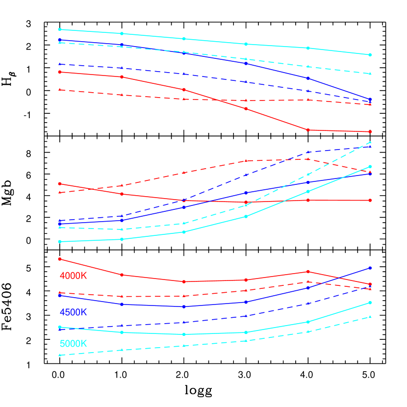
Figure 4: Comparison of MARCS (solid lines) and Munari (dashed lines) models (scaled solar, [Fe/H]=0.0) for H$\beta$, Mg$b$ and Fe5406, at effective temperatures $T_{eff}$=4000K (red), 4500K (blue), 5000K (cyan).

We decided not to attempt to include (or create) lower temperature high resolution spectra because we are concerned about possible inconsistencies between stellar atmosphere models from different sources. Figure 4 shows a comparison between line strengths derived from the Munari et al. (2005) spectra (based on ATLAS9 model atmospheres) and corresponding spectra from the MARCS database – we compare strengths of the H$\beta$, Mg$b$ and Fe5406 lines since we will be using these extensively in our more detailed analyses later in this paper. It can be seen that for all 3 lines there are significant offsets, and that the behaviour becomes increasingly discrepant between the 2 models as the temperature decreases. We note that these comparisons were done using the MARCS models available as of May 2008. New low temperature MARCS models are currently being produced (Gustafsson et al., 2008) – we will investigate these as they become available and may include them in our integrated spectra at a later date. We note here that this low temperature regime also includes cool AGB stars, for which no realistic models currently exist.

The effect of not including stars with $T_{eff}<3500$K in the high resolution integrated spectra is illustrated in Figure 5. Here we use the low resolution spectra to separate out the flux contribution from these stars, for two representative SSPs, and plot the percentage of the total flux coming from $T_{eff}<3500$K as a function of wavelength. It can clearly be seen that the flux contribution from these stars only becomes significant at wavelengths longer than the bandpasses of the main Lick-style indices, e.g. H$\beta$, Mg$b$ and various Fe lines (see 2.2.1).

It is expected that high metallicity SSPs will be most affected by this low temperature cut-off in the spectral library, since a larger portion of their isochrones fall in the $T_{eff}<3500$K regime than for low metallicity SSPs. As a test of the maximum likely effect on various diagnostic lines (see next section for definitions), we mimicked the effect of a $T_{eff}=3500$K cut on a $Z$=0.04 (i.e. $\sim$ twice solar), 10 Gyr SSP by taking a 10 Gyr, $Z$=0.001 ($\sim\frac{1}{20}$ solar) isochrone and imposing a temperature cut at $T_{eff}=$4130K. This temperature cut corresponds to approximately the same evolutionary point on the isochrone as a $T_{eff}=3500$K cut for the higher metallicity SSP. We then created an integrated spectrum for this ‘truncated’ $Z$=0.001 SSP and compared the derived line indices with those derived from the integrated spectrum for the full SSP at the same age and metallicity. For the ‘truncated’ spectrum, the H$\beta$ index (the main age indicator – see next section) was $\sim$ 0.1 higher than that of the full spectrum. This corresponds to an age difference of $\sim$ 1 Gyr, and goes in the sense that the truncated spectrum looks too young. There are various metallicity indicators (see next section) – for the main [Fe/H] indicator we use here, Fe5406, the line strength is slightly lower than for the full spectrum, which would result in an underestimate of the true [Fe/H] by $\sim$ 0.05 dex. We repeated this test for a 3 Gyr model and found similar absolute offsets, which would result in slightly smaller effects on the inferred age, at the level of $\sim$ 0.5 Gyr.

It should be noted that the issue of ‘missing flux’ at low temperatures, and its associated effect on line indices, is not a problem specifically associated with the use of theoretical spectral libraries. It is also very relevant to any population synthesis techniques which rely on empirical spectra, since there are very few local stars at these low temperatures, particularly at low metallicity.

2.2.1 Line indices: behaviour as a function of age and metallicity

All the line indices discussed in this paper are defined by the bandpasses tabulated in Trager et al. (1998, i.e. the 21 classical Lick/IDS indices). The quoted line strengths, and hence those displayed in plots, were obtained using the LECTOR programme by A. Vazdekis and are those directly measured on the spectra, i.e. they are not transformed onto the Lick system.

Before discussing the behaviour of various line indices it is worth remembering the distinction between iron abundance, quantified here as [Fe/H], and total metallicity, $Z$. For scaled solar models, all metal abundances scale as for the sun, whilst in $\alpha$-enhanced models the $\alpha$ element abundances are increased relative to Fe. Hence at fixed $Z$, the $\alpha$-enhanced models have a lower [Fe/H] than the corresponding scaled solar models. As an example, the BaSTI scaled solar models with $Z$=0.0198 (the solar value) have [Fe/H]=+0.06, whilst the corresponding $\alpha$-enhanced models have [Fe/H]=$-$0.29. In the following discussion we will focus in detail on specific line indices which we will be using diagnostically to determine iron content [Fe/H], total metallicity $Z$, and age.

The left-hand panel of Figure 6 shows grids of H$\beta$ vs. Fe5406 derived from our SSP integrated spectra for a range of metallicities and ages, as detailed in the figure caption. The figure includes both the scaled solar and $\alpha$-enhanced grids and clearly demonstrates that the Fe5406 line is predominantly a tracer of iron abundance, [Fe/H], since the 2 grids closely correspond along lines of very similar [Fe/H], and is generally insensitive to the degree of $\alpha$ enhancement. This is not the case for other Fe line indices we have tested, which also include other dominant elements, as listed in Trager et al. (1998, their Table 2). Although our line indices are not converted onto the Lick system, this sensitivity of the Fe5406 line to Fe only is similar to that noted in other studies which do utilize indices on the Lick system, e.g. Lee & Worthey (2005) and Korn et al. (2005).

The right-hand panel of Figure 6 shows similar grids for H$\beta$ vs. [MgFe], where [MgFe] is defined as $\sqrt{{\rm<Fe>}\times{\rm Mg}b}$ and $<$Fe$>$=$\frac{1}{2}$(Fe5270+Fe5335). It can clearly be seen that [MgFe] is sensitive to total metallicity, $Z$, since the scaled solar and $\alpha$-enhanced grids almost exactly correspond along lines of constant $Z$ across a wide metallicity range. An important trend to note in this plot is the behaviour of the H$\beta$ line which, at fixed total metallicity $Z$ and age, is stronger in the $\alpha$-enhanced models than the scaled solar ones. This behaviour of the H$\beta$ line strength is qualitatively similar to that found by Tantalo et al. (2007), who used high resolution spectra to determine response functions which are used in conjunction with existing fitting functions to ‘correct’ solar scaled indices to the appropriate $\alpha$-enhancement (effectively, an update of the method used by Tripicco & Bell 1995). However we note here that the recent work of Coelho et al. (2007), discussed in Section 2.1.1, seems to display the opposite trend in the behaviour of H$\beta$ with respect to $Z$ (see discussion below).

These 2 figures seen together (i.e. the 2 panels of Figure 6) illustrate very well the difficulty in predicting ages from the H$\beta$ line without also having other information, in particular, the degree of $\alpha$ enhancement. From our models it seems that the H$\beta$–Fe5406 combination can be used to unambiguously determine age and [Fe/H], but yields no information about the degree of enhancement. Conversely, using H$\beta$–[MgFe] alone could result in spurious ages unless the appropriate level of $\alpha$ enhancement is determined by other means. Hence the diagnostic use of a single index-index diagram is not recommended.

In Figure 7 (left-hand panel) we show the corresponding grids for H$\beta$ vs. Mg$b$ which demonstrate the sensitivity of the Mg$b$ index to the degree of $\alpha$ enhancement (note that in our models this is fixed at $[\alpha$/Fe]=0.4). Qualitatively similar behaviour is also seen by Schiavon (2007). However, this is a difficult grid to use diagnostically because the sensitivity to changing [Fe/H] and $Z$ are impossible to disentangle from this grid alone and hence, in our later analysis, we will utilise the Fe5406–[MgFe] plane, illustrated in the right-hand panel of Figure 7. In this plane, the lines of constant age are almost completely degenerate, however the scaled solar and $\alpha$-enhanced grids are clearly separated. Using a combination of 3 grids – H$\beta$ vs. Fe5406, H$\beta$ vs. [MgFe], and Fe5406 vs. [MgFe] – it should be possible to disentangle age, total metallicity $Z$, [Fe/H] and the degree of $\alpha$ enhancement, as we demonstrate in Section 3.1.

We compared the line strengths derived from our high resolution integrated spectra to those of Coelho et al. (2007), a recent study which uses a method most similar to ours to produce integrated spectra for a range of SSPs (see Section 2.1.1 for a comparison with their colors). The upper left panel of Figure 8 shows our scaled solar H$\beta$ vs. Fe5406 grid with the Coelho data superimposed for [Fe/H]=0.0 (ages 3-12 Gyr). There is reasonably good agreement between their models and ours in the general locus of points along the [Fe/H]=0.0 line, however there are obvious offsets in H$\beta$ which would cause a discrepancy in predicted ages. In general, their scaled solar grid lies at higher H$\beta$ values than ours and so for a fixed (observed) data point we would predict younger ages. The upper right hand panel of Figure 8 shows the full grid of H$\beta$ vs. Fe5406 from the Coelho models (note, only 3 metallicities are currently available) – this figure seems to show the opposite trend in the behaviour of $H\beta$ with respect to $\alpha$-enhancement compared to our models, as mentioned above.

We have no obvious explanation for this difference in behaviour but it should be noted that, although Coelho et al. (2007) use a method which is qualitatively similar to ours to produce integrated spectra, they are using different underlying stellar models and a different spectral library. In particular, we note here that the isochrones used in the Coelho models differ signficantly from the BaSTI ones when similar ages and metallicities are compared. In general, their RGBs are at cooler temperatures than the BaSTI ones, by up to $\sim$ 200K. Also the temperature at the turn off (TO) displays significant differences in behaviour, e.g. at old ages, the BaSTI isochrones have hotter TOs, whilst at intermediate and young ages this trend is reversed, and the BaSTI TOs are cooler. Coelho et al. (2007) also include some low temperature spectra in their models, generated using the MARCS model atmospheres, in order to cover all evolutionary stages – this enables them to compute broadband colors from their high resolution spectra, whilst we use our low resolution spectra for this. They also compute models for different values of total metallicity $Z$ to ours, meaning that a comparison of grids (i.e. with a range of ages and metallicities) is very difficult – only their scaled solar, [Fe/H]=0.0 models are directly comparable with ours.

For the interested reader, we also include a similar comparison with the fitting-function based models of Thomas et al. (2003) – these are displayed in the lower panels of Figure 8. By definition, fitting-function based models are on the Lick system and so we have modified the tabulated H$\beta$ and Fe5406 values by 0.13 and 0.2 respectively, according to the prescription of Bruzual & Charlot (2003, their Table 6), to make them directly comparable with indices derived from flux calibrated spectra, as used in our work.

We note here that all of our models presented so far in this paper have used the BaSTI non-overshooting models with a value for the Reimers mass loss parameter of $\eta$=0.2. The effect of varying $\eta$ will be discussed in the next section.

3 Comparisons with resolved stellar clusters

Any stellar population synthesis model should be tested against resolved populations with independent estimates of chemical composition and age. Star clusters belonging to the Galaxy are the obvious choice, because their chemical composition can be determined from spectroscopy, and theoretical isochrones matched to the observed color-magnitude diagram (CMD) provide an estimate of the age. Ideally, the analysis of integrated colors and spectra by means of population synthesis methods should provide a chemical composition and age consistent with the inferences from spectroscopy and the CMD (see, e.g. Gibson et al., 1999; Vazdekis et al., 2001; Schiavon, 2007, and references therein).

To this purpose one can make use of the Schiavon et al. (2005) library of integrated spectra of 40 Galactic globular clusters, plus the integrated spectrum of the Galactic open cluster M67 (Schiavon et al., 2004a). Each of the globular cluster integrated spectra covers the range $\sim 3350-6430$Å, with $\sim$ 3.1Å (FWHM) resolution, and one can potentially attempt fits to the whole sample of spectra, comparing the results derived from diagnostic lines to those derived from isochrone fitting to the observed CMD. There are however some serious issues that one has to take into account when interpreting the results of these comparisons.

The first problem is the [Fe/H] estimates of the clusters. There are large discrepancies between the widely employed Zinn & West (1984) and Carretta & Gratton (1997) scales. For example, well studied objects like M3 and M5 show differences of $\sim$0.3 dex between the two [Fe/H] estimates. A third [Fe/H] scale by Kraft & Ivans (2003) based on FeII lines shows very large differences compared to the previous two sets of estimates in the low metallicity regime. As an example, a well studied metal poor cluster like M68 displays a $\sim$ 0.4 dex range of [Fe/H] values when these three different [Fe/H] scales are employed. Taking a mean value of the various determinations for each cluster does not make much sense, given that the differences among the authors are mainly systematic. In addition, [$\alpha$/Fe] spectroscopic estimates do not exist for many clusters.

The second issue is the presence of the well known CN and ONa anticorrelations in the metal mixture of stars within a single cluster (see, e.g., the review by Gratton et al., 2004, and references therein). There is now convincing evidence that C, N, O, Na – and sometimes also Mg and Al – display a pattern of abundance variations superimposed onto a normal $\alpha$-enhanced heavy element distribution. Negative variations of C and O are accompanied by increased N and Na abundances. There is also now general agreement that these abundance patterns are of primordial origin. This means that the integrated spectrum of a cluster is composed of individual spectra with a range of values for the very important CNONa elements, whereas the Fe abundance is essentially constant for all stars. It is therefore very difficult to interpret the strength of all line indices affected by these 4 elements, given that in a cluster the exact proportions of stars with a certain set of CNONa abundances, and their location along the CMD, are known only for small samples of objects.

The third issue is related to the morphology of the horizontal branch (HB). As is well known (see, e.g. Schiavon et al., 2004b), the presence of blue HB stars affects the Balmer lines, which can produce spuriously young ages for clusters with an extended blue HB if this is not included in the theoretical modelling. A detailed synthetic modelling of the HB color extension for each of the observed clusters is therefore in principle necessary. Whilst this is possible in principle, it is difficult to implement in practice and would be computationally very time consuming to model all the different possibilities. This approach also assumes that one knows, a priori, the appropriate morphology required – this of course is not possible for unresolved stellar clusters. The color of the HB is determined by the mass loss history of RGB stars when the initial chemical composition is fixed. In the theoretical isochrones, this is modelled using the Reimers mass loss law, and the mass loss parameter $\eta$ is a free parameter in the models, which is set at some fixed value for each isochrone. This means that for any particular isochrone, all the stars on the HB have essentially the same mass and hence start their evolution from the Zero Age HB all with the same color. For any fixed $\eta$ value, higher metallicity SSPs have a red clump of stars along the HB. The distribution of objects along the HB becomes progressively bluer when the metallicity decreases, provided that $\eta$ is unchanged. In Galactic globular clusters however, the mean color and color extension of the HB is often not correlated to the cluster metallicity, and additional chemical or environmental parameters that directly or indirectly affect the mass distribution along the HB, must be at play (see e.g. Caloi & D’Antona, 2005; Recio-Blanco et al., 2006, and references therein). If $\eta$ is fixed at a higher value in the models, the blue extension of the HB becomes more extreme at low metallicity, particularly for old ages (see discussion below).

A final issue is the existence of blue stragglers in the CMDs of Galactic globular clusters, i.e. a plume of stars brighter and generally bluer than the TO, thought to be created through mass transfer in a binary system or through direct collision of 2 stars. Integrated spectra that include only the contribution of single star evolution miss this component, causing potential biases in their age estimates.

Keeping in mind all these limitations, we first compare the whole globular cluster (GC) spectral library by Schiavon et al. (2005) to our high resolution spectra calculated with both $\eta=0.2$ and $\eta=0.4$. We have measured indices on the GC spectra in exactly the same way as for our model spectra. We note here that the Schiavon et al. (2005) data set includes multiple observations for several clusters – in the following plots all the data points are shown. To minimize the effect of the CNONa anticorrelations on the comparison, we consider first the Fe5406$-$[MgFe] plane to estimate [Fe/H] (which is constant among all stars in a cluster) and the degree of $\alpha$-enhancement from our theoretical spectra. As seen in section 2.2.1, [MgFe] is sensitive to the global metallicity of the stellar population, but not to the exact distribution of the metals, and therefore the Fe5406$-$[MgFe] diagram – insensitive to age for old stellar populations – depends on the relationship between the global metallicity $Z$ and the iron content in the population. Given that at fixed [Fe/H] an $\alpha$-enhanced mixture has a larger $Z$ compared to a scaled-solar one, the position of a cluster in this diagram is related to the degree of $\alpha$-enhancement in the spectra of its stars. A possible complication is that the CNONa anticorrelation modifies the baseline $\alpha$-enhanced metal mixture in a fraction of stars within the cluster. However, if the sum of C+N+O (which makes up a substantial fraction of the total metals) is unaffected by the abundance anomalies (as seems to be the case within current observational errors, see, e.g. Carretta et al. 2005) the relation between [Fe/H] and $Z$ is unchanged, and the Fe5406$-$[MgFe] diagram still provides an estimate of the degree of $\alpha$-enhancement in the baseline chemical composition of the cluster as a whole.

Figure 9 shows all the Schiavon data points in the Fe5406–[MgFe] plane, with lines of 14 Gyr (constant) age derived from our scaled solar and $\alpha$-enhanced spectra, in the metallicity range $-1.8<{\rm[Fe/H]}<+0.06$. In general, the data points fall exactly between the scaled solar and $\alpha$-enhanced lines indicating that most of them are probably $\alpha$-enhanced to some extent, as expected. The group of points at the top of the grid represents 2 clusters only – NGC6528 (for which there are 6 observations) and NGC 6553, which are the 2 most metal rich clusters in the data set at [Fe/H]$\sim-0.2$. The 4 points at the bottom left of the grid represent 2 observations each of NGC 2298 and NGC 7078, the 2 most metal poor clusters at [Fe/H]$\sim-2.0$. Hence we maintain that this grid is a good first indicator of [Fe/H], and also provides an estimate of the degree of $\alpha$ enhancement.

Once [Fe/H] and the degree of $\alpha$-enhancement are established we can then use the H$\beta$–Fe5406 plane to estimate the cluster ages – Figure 10 shows the same GC data points on our $\alpha$-enhanced grid, calculated using $\eta$=0.2. Whilst the intermediate metallicity clusters generally span the 10-14 Gyr age range (within the errors), it can be seen that the more metal poor clusters all seem to scatter to higher ages. This is most likely to be due to the blue extent of their HBs, as discussed above. To illustrate the potential effect of having extended blue HBs due to increased mass loss on the RGB, we have overplotted the 14 Gyr line calculated using $\eta$=0.4 – this clearly demonstrates the large increase in the strength of the H$\beta$ line which can lead to spuriously young ages. We note that the trend of this $\eta$=0.4 line, i.e. the rise to a peak in H$\beta$ at some intermediate metallicity and then a decrease towards lower metallicities, is not unexpected. For the most metal poor old clusters, the horizontal branch can develop a very long blue tail which extends down to magnitudes almost as faint as the turn off in optical bands. Thus although the individual stars still exhibit strong H$\beta$ due to their very hot temperatures, their contribution to the overall continuum flux decreases at the wavelength of H$\beta$ (which is in the middle of the $B$-band) at the lowest metallicities.

3.1 Case study: 47 Tuc

We have performed a more detailed comparison for the case of 47 Tuc, which is one of the clusters in the Schiavon et al. (2005) database. This cluster has a reasonably well established [Fe/H]. Carretta & Gratton (1997) find [Fe/H]=$-0.70\pm 0.07$, Zinn & West (1984) give [Fe/H]=$-0.71\pm 0.08$, while Kraft & Ivans (2003) obtain between $-$0.78 and $-$0.88 depending on the assumed $T_{eff}$ scale, based on the equivalent widths of FeII lines measured from high-resolution spectra of giants. More recent high resolution spectroscopy by Carretta et al. (2004) gives an estimate consistent with that of Carretta & Gratton (1997), while Koch & McWilliam (2008) obtain [Fe/H]=$-0.76\pm 0.01\pm 0.04$. Measurements of $\alpha$-element abundances by Carretta et al. (2004) and Koch & McWilliam (2008) give $\alpha$ enhancement, [$\alpha$/Fe], of the order of $\sim 0.3-0.4$ dex on average.

Figure 11 displays a fit to the $BV$ data by Stetson (2000) with the BaSTI $\alpha$-enhanced, $\eta$=0.2 isochrone and ZAHB, with [Fe/H]=$-$0.7 and an age of 12 Gyr. A more formal determination of the age and associated errors has been obtained using the $\Delta V$ method described in, e.g., Salaris & Weiss (1997, 1998). This method employs the difference in $V$ magnitude between the Zero Age HB (ZAHB) and the turn off (TO), designated $\Delta V$, as an age indicator. This quantity turns out to be weakly sensitive to the cluster metallicity, so that errors on the age estimate are dominated by errors on the determination of the ZAHB and TO magnitudes (see the discussion in Salaris & Weiss 1997). We obtain for 47 Tuc an age $t=12\pm$1 Gyr where in the error budget we have included the small contribution of a $\pm$0.2 dex uncertainty around the reference [Fe/H]=$-$0.7.

A comparison of the 47 Tuc line indices with those derived from the theoretical spectra (computed with $\eta$=0.2) in the Fe5406$-$[MgFe] and H$\beta-$Fe5406 diagrams is included in Figures 9 and 10. We have estimated representative error bars for 47 Tuc, which will be approximately the same for all the GC data points. These include contributions from the measurement of the line indices on the observational data as given by the LECTOR program, an estimate of the intrinsic observational error (there is only one observation of 47 Tuc), and a small contribution due to the difference in resolution between the data and the models. Within the error bars of the observed indices, our BaSTI integrated spectra yield [Fe/H], [$\alpha$/Fe] and age estimates in agreement with the results from high resolution spectroscopy of individual stars and from the CMD age.

We have then checked the extent of possible biases introduced by the theoretical representation of the cluster HB, which differs from the observed one. To this purpose we have considered the Fe5406, [MgFe] and H$\beta$ values obtained from a 14 Gyr old, $\eta$=0.2, [Fe/H]=$-$0.7 theoretical spectrum. We have then computed an integrated spectrum for the same age and [Fe/H], but considering a synthetic HB (obtained as described in Salaris et al. 2007) that precisely matches the color extension observed in 47 Tuc. The resulting Fe5406, [MgFe] and H$\beta$ values are practically unchanged compared to the $\eta$=0.2 case – the increase in H$\beta$ is $<$ 0.04, corresponding to an age difference of $<$ 0.5 Gyr, and well within the observational error, whilst Fe5406 and [MgFe] are negligibly changed.

As a second check we have estimated the effect of the blue stragglers present in the cluster CMD. According to the estimates by Piotto et al. (2002), the ratio of blue stragglers to the number of HB stars is about 0.15, one of the lowest fractions within the Galactic globular cluster system. To determine an upper limit of their effect on the indices used in our analysis, we have added to the 14 Gyr old [Fe/H]=$-$0.7, $\eta$=0.2 integrated spectrum, the contribution of a clump of Zero Age MS stars 1.5 mag brighter than the isochrone TO, which is the approximate position of the bluest and brightest blue stragglers in the $BV$ CMD by Sills et al. (2000). Their number is assumed to be 15% of the number of HB stars predicted by the models. All line indices measured on the resulting integrated spectrum are practically unchanged compared to the reference values, with differences of no more than 0.01 in any of the diagnostic indices used here.

3.2 Case study: M67

As a second detailed test, we have considered the open cluster M67. Schiavon et al. (2004a) have created a representative integrated spectrum for M67, built up from observations of spectra of individual stars in the cluster (about 90 objects) that sample as well as possible the CMD from the lower MS to the tip of the RGB and the He-burning (red clump) phase. Some local field stars are also included to better sample some regions of the cluster CMD not well represented by the M67 data alone. Schiavon et al. (2004a) assigned a mass to each of the sample stars by using inputs from theoretical isochrones, and then the individual spectra were coadded with weights given by an adopted IMF (they employ a Salpeter IMF). The contribution of objects with masses below $\sim$0.85 $M_{\odot}$ (below the faintest objects whose spectrum is included in the Schiavon et al. 2004a analysis) has been included by Schiavon (2007) using inputs from theoretical models. The corrections that need to be applied to line indices measured on their published M67 spectrum to account for this (their Table 11) have been included in our analysis. The contribution of blue stragglers is excluded from the spectrum we employ in the comparisons that follow.

For this cluster the spectroscopic investigations by Tautvaišiene et al. (2000), Yong et al. (2005), Randich et al. (2006) and the analysis by Taylor (2007), all give [Fe/H]$\sim 0.0$. The best age estimate obtained by fitting our [Fe/H]=+0.06 BaSTI non-overshooting isochrones to Sandquist (2004) photometry is $t$=4.0 Gyr. The inclusion of overshooting has only a marginal effect at this age, increasing $t$ to 4.2 Gyr. The quality of the fit is very similar, with a small preference for the non-overshooting case, which we display in Figure 12.

A comparison of the M67 line indices with those derived from our scaled solar non-overshooting grid (computed with $\eta$=0.2, but at the age of M67 the choice of $\eta$ is irrelevant) in the H$\beta-<$Fe$>$ diagram is displayed in Figures 13. We used $<$Fe$>$ instead of the Fe5406 line here because the wavelength coverage of the M67 spectrum is slightly less than for the GC sample, cutting off at 5396Å. We have not assigned error bars to the data point on this plot as it not trivial to quantify them – they must however be at least as large as the error bars estimated for the GC data, and some other potential contributory factors are discussed below. Whilst the age inferred from this diagram is consistent with the CMD age, the predicted [Fe/H] is lower than the spectroscopic value by about 0.2 dex. There are some important factors which we think may contribute to this discrepancy which we address in the following discussion.

One important point to consider is that M67 spectrum does not come from observations of the cluster integrated light (as is the case for the GC data set), rather it has been built in the same way as theoretical integrated spectra are built, starting from an isochrone. Each point along the isochrone has been assigned an appropriate spectrum, and the contributions of the individual spectra weighted by the chosen IMF. The BaSTI isochrones include more than 2100 points to sample masses above 0.85$M_{\odot}$ – a very fine coverage – whereas the M67 spectrum has been computed using a much smaller number of individual representative stars. To get a handle on the effect introduced by the sampling used for the observed spectrum, we have computed two integrated spectra for the same age of 4.0 Gyr ([Fe/H]=0.06, scaled solar non-overshooting models). The first one has been obtained as usual, whereas for the second spectrum the resolution of the isochrone for masses above 0.85$M_{\odot}$ has been degraded to include only 90 points. The spacing of these points has been chosen to reproduce as well as possible the $V$ magnitude distribution of the stars used by Schiavon et al. (2004a) (we have assumed a distance modulus $(m-M)_{0}$=9.67, as obtained from the isochrone fitting). We find a non-negligible difference between line indices computed with these two different isochrone samplings. The value of the difference between the fine sampling and the coarse sampling spectrum has then to be added to the measured values for M67, in order to have a more consistent comparison with the theoretical grid. The direction in which the data point moves in the the H$\beta-<$Fe$>$ plane after applying this correction is indicated on Figure 13 by the arrow. The H$\beta$ value decreases, implying a slightly older age, although this may not be significant within the observational errors. Interestingly, all the Fe indicators move to significantly higher values, increasing the inferred [Fe/H] by as much as 0.2 dex and putting the predicted [Fe/H] more in line with the spectroscopic value.

This test highlights some subtle issues affecting the creation of SSPs which can have non-trivial effects on their derived integrated properties and spectra. We remind the reader that the method of populating an isochrone to create an SSP used here (and in other population synthesis studies) is an analytical one, in which the isochrone is effectively treated as a continuous function. This method is strictly correct only in the limit of an infinite number of objects in the stellar system being modelled, but is the appropriate method to use when modelling an unresolved population. In practice, an isochrone consists of a discrete number of evolutionary points (EPs), all of which are assigned a spectrum when the analytical method is used. However, the number of defined EPs, resulting in coarse or fine sampling of the isochrone, can make a difference to the resultant integrated properties, as demonstrated above.

A further refinement in the modelling of the integrated properties of observed stellar clusters can be made by populating the isochrone with a discrete number of stars appropriate to the type of cluster (using an IMF, as before). The Web tool provided on the BaSTI database which creates synthetic CMDs for resolved populations (SYNTHETIC MAN) populates isochrones in this way, with the number of stars in the simulation being determined by the user. When the number of stars in a particular simulation is not large enough to populate every EP on the isochrone (which is already true for typical $10^{5}-10^{6}~{}M_{\odot}$ Galactic globular clusters) statistical fluctuations of star counts will arise. This means that an ensemble of SSPs all with the same total mass, age and initial chemical composition will display a range of integrated magnitudes and colors, that increases (for a fixed value of ${\rm M_{t}}$) when moving towards longer wavelengths, which are dominated by the shorter-lived (hence more sparsely populated) RGB and AGB phases. Preliminary tests by us have shown that there are also non-negligible effects on integrated spectra produced in this way and that a significant scatter is seen in derived line indices when the number of stars in the simulations corresponds to a total mass less than $\sim 2\times 10^{5}M_{\odot}$ (i.e. roughly the size of a typical GC and larger than most open clusters). In particular, one significant factor seems to be the exact location of the brightest star populating the RGB, which can easily vary by several tenths of a magnitude when modelling open clusters like M67.

All these issues, and particularly the effects of statistical fluctuations on integrated spectra and derived line indices, will be explored further in a subsequent paper.

4 Summary

In this 4th paper in the BaSTI series we have presented a new set of low and high resolution synthetic spectra based on the BaSTI stellar models, covering a large range of SSPs, for both scaled solar and $\alpha$ enhanced metal mixtures. This enables a completely consistent study of the photometric and spectroscopic properties of both resolved and unresolved stellar populations, and allows us to make detailed tests on specific factors which can affect their integrated properties.

• We have produced low resolution spectra suitable for deriving broadband magnitudes and colors in any photometric system and ensured that the derived colors are fully consistent with those predicted from the BaSTI isochrones.

• We have produced high resolution spectra suitable for studying the behaviour of line indices and tested them against a large sample of Galactic globular clusters, making particular note of the effect of horizontal branch morphology.

• We have tested the global consistency of the BaSTI models by making detailed comparisons between ages and metallicities derived from isochrone fitting and from line index strengths for the Galactic globular cluster 47 Tuc and the open cluster M67.

• We find non-negligible effects on derived line indices caused by statistical fluctuations, which are a result of the specific method used to populate an isochrone and assign appropriate spectra to individual stars.

Appendix A Appendix

Upon publication of this paper, the official BaSTI website (http://193.204.1.62/index.html) will be expanded to include integrated spectra (low and high resolution), magnitudes and mass-to-light (ML) ratios for SSPs (normalized to 1$M_{\odot}$ of stars formed during the burst of star formation) covering the full range of ages, chemical compositions, choices of mass loss and mixing included in the database. A full summary of the parameter space covered by BaSTI can be found in Cordier et al. (2007). Integrated magnitudes and ML ratios will be provided for $UBVRIJHKL$ filters. Additional photometric systems can be easily accounted for by convolving the BaSTI low resolution integrated spectra with the appropriate filter response curves, and using an appropriate normalizing spectrum (a Vega synthetic spectrum is also included in BaSTI). ML-ratio files also tabulate the amount of mass locked into the various types of remnants for each SSP, to help determine ML-ratios in any arbitrary photometric system. We remind the reader that the ML-ratio of a stellar population is customarily defined as the ratio between the integrated luminosity in a given passband (in solar units) divided by the integrated stellar mass (in solar units) contained in stars, including all remnants like white dwarfs (WDs), neutron stars (NSs) and black holes (BHs). To compute the solar luminosity in the $UBVRIJHKL$ we have adopted the following set of solar absolute magnitudes: $M_{U}=5.66,M_{B}=5.49,M_{V}=4.82,M_{R}=4.45,M_{I}=4.10,M_{J}=3.68,M_{H}=3.31,M_{K}=3.28,M_{L}=3.26$. The mass contained in WD, NS and BH remnants has been computed by assuming an initial-final-mass (IFMR) relation in addition to the IMF. For WDs with a carbon-oxygen core we employed the IFMR obtained from our AGB modelling. The upper initial mass limit for the production of carbon-oxygen WDs (the so-called $M_{up}$) is also obtained from our stellar models. For initial masses between $M_{up}$ and 10 $M_{\odot}$ we considered typical oxygen-neon core WDs with masses of 1.3$M_{\odot}$. Initial masses between 10 and 25 $M_{\odot}$ are assumed to give rise to 1.4$M_{\odot}$ NSs, whereas for progenitors above 25$M_{\odot}$ we consider a final state as black holes with mass equal to $1/3$ of the initial mass.

Figure 1: Sample low resolution (upper panel) and high resolution (lower panel) integrated spectra from scaled solar, $Z$=0.0198 (the solar value) models. Ages displayed are 3 and 10 Gyr, which are the upper and lower spectra respectively on each plot.

Figure 2: SSP colors from BaSTI models. Solid lines are the scaled solar models for [Fe/H]=$+0.06$, $-0.66$ and $-1.27$ (upper, middle and lower lines respectively on each plot). Dashed lines are the $\alpha$-enhanced models for [Fe/H]=$+0.05$, $-0.70$ and $-1.31$.

Figure 3: Comparison of BaSTI colors (solid lines) with those from Coelho et al. (2007) (dashed lines). The BaSTI colors are from our scaled solar [Fe/H]=+0.06 and $\alpha$-enhanced [Fe/H]=+0.05 models. The Coelho models are both for [Fe/H]=0.0.

Figure 5: Percentage of flux in stars with $T_{eff}<$ 3500K for 2 representative SSPs. Bandpasses for H$\beta$, Mg$b$ and Fe5406 are marked with the dotted lines.

Figure 6: Grids of H$\beta$ vs. Fe5406 (left panel) and [MgFe] (right panel) measured on our high resolution spectra as described in the text. The solid line/circles are the scaled solar grid, the dashed line/open squares are the $\alpha$-enhanced grid. Scaled solar models are for $Z$=0.0003, 0.0006, 0.001, 0.002, 0.004, 0.008, 0.0198, 0.04 (corresponding to [Fe/H]=$-$1.79, $-$1.49, $-$1.27, $-$0.96, $-$0.66, $-$0.35, +0.06, +0.40) and $\alpha$-enhanced models are for $Z$=0.0006, 0.002, 0.004, 0.008, 0.0198, 0.04 (corresponding to [Fe/H]=$-$1.84, $-$1.31, $-$1.01, $-$0.70, $-$0.29, +0.05). Metallicity increases from left to right. Ages (increasing from top to bottom) are 1.25, 3, 6, 8, 10 and 14 Gyr.

Figure 7: H$\beta$ vs. Mg$b$ (left panel) and Fe5406 vs. [MgFe] (right panel). Models and symbols are as for Figure 6.

Figure 8: Comparison of our H$\beta$ vs. Fe5406 grids with those of Coelho et al. (2007) (upper panels) and Thomas et al. (2003) (lower panels). The left panels show the Coelho (upper) and Thomas (lower) [Fe/H]=0.0, scaled solar models for ages 3-12 Gyr superimposed on our scaled solar, H$\beta$ vs. Fe5406 grid. Upper right shows the Coelho grids for scaled solar (solid) and $\alpha$-enhanced (dashed lines) for [Fe/H]= $-$0.5, 0.0 and +0.2. Lower right shows TMB03 scaled solar grids for [Fe/H]=$-$0.33, 0.0, 0.35 (solid) and $\alpha$-enhanced ([$\alpha$/Fe]=0.3), [$Z$/H]=0.0, 0.35, 0.67, corresponding to [Fe/H]=$-$0.28, 0.06, 0.38 (dashed).

Figure 9: Fe5406 vs. [MgFe] from our scaled solar and $\alpha$-enhanced 14 Gyr spectra (solid and dashed lines, respectively) joined at approximately equal [Fe/H] (dotted lines) for [Fe/H] $\sim$ +0.06, $-$0.3, $-$0.7, $-$1.0, $-$1.3, $-$1.8 (decreasing from top to bottom). Open circles are the Galactic globular cluster data from Schiavon et al. (2005) – 47 Tuc is represented by the solid square, with an estimated typical error bar.

Figure 10: H$\beta$ vs. Fe5406 grid for our $\alpha$-enhanced models ([Fe/H]=$-$1.84, $-$1.31, $-$1.01, $-$0.70, $-$0.29, +0.05) with GGC data from Schiavon et al. (2005) overplotted – symbols as for Figure 9. The grid shown is calculated using mass loss parameter $\eta$=0.2. The dashed line is for the 14 Gyr models only and was calculated using $\eta$=0.4, this illustrates the effect of a very extended blue horizontal branch on the predicted H$\beta$.

Figure 11: Isochrone fit to 47 Tuc (data from Stetson, 2000). The best fit to a 12 Gyr, [Fe/H]=$-$0.7, $\alpha$-enhanced isochrone yields a distance modulus of $(m-M)_{0}$=13.28, for an assumed reddening of $E$(B-V)=0.02, in agreement with the empirical main-sequence fitting result of Percival et al. (2002).

Figure 12: Isochrone fit to M67 (data from Sandquist, 2004). The best fit to a scaled solar, non-overshooting, [Fe/H]=0.06 isochrone, yields an age of 4.0 Gyr and a distance modulus of $(m-M)_{0}$=9.67, for an assumed reddening of $E$(B-V)=0.02, in agreement with the empirical main-sequence fitting result of Percival & Salaris (2003).

Figure 13: Scaled solar grid for H$\beta$ vs. $<$Fe$>$ with the M67 data point, calculated as described in the text. The arrow shows the approximate direction and distance the point would move if the effects of statistical fluctuations were taken into account.

References

- Alonso et al. (1999) Alonso, A., Arribas, S., & Martínez-Roger, C. 1999, A&AS, 140, 261
- Barker et al. (2007) Barker, M. K., Sarajedini, A., Geisler, D., Harding, P., & Schommer, R. 2007, AJ, 133, 1138
- Bruzual & Charlot (2003) Bruzual, G. & Charlot, S. 2003, MNRAS, 344, 1000
- Caloi & D’Antona (2005) Caloi, V. & D’Antona, F. 2005, A&A, 435, 987
- Carrera et al. (2008) Carrera, R., Gallart, C., Hardy, E., Aparicio, A., & Zinn, R. 2008, AJ, 135, 836
- Carretta & Gratton (1997) Carretta, E. & Gratton, R. G. 1997, A&AS, 121, 95
- Carretta et al. (2004) Carretta, E., Gratton, R. G., Bragaglia, A., Bonifacio, P., & Pasquini, L. 2004, A&A, 416, 925
- Carretta et al. (2005) Carretta, E., Gratton, R. G., Lucatello, S., Bragaglia, A., & Bonifacio, P. 2005, A&A, 433, 597
- Cassisi et al. (2001) Cassisi, S., Castellani, V., & Ciarcelluti, P. 2001, Memorie della Societa Astronomica Italiana, 72, 743
- Cassisi et al. (2004) Cassisi, S., Salaris, M., Castelli, F., & Pietrinferni, A. 2004, ApJ, 616, 498
- Castelli & Kurucz (1994) Castelli, F. & Kurucz, R. L. 1994, A&A, 281, 817
- Castelli & Kurucz (2003) Castelli, F. & Kurucz, R. L. 2003, in IAU Symposium, Vol. 210, Modelling of Stellar Atmospheres, ed. N. Piskunov, W. W. Weiss, & D. F. Gray, 20P
- Coelho et al. (2007) Coelho, P., Bruzual, G., Charlot, S., Weiss, A., Barbuy, B., & Ferguson, J. W. 2007, MNRAS, 382, 498
- Cordier et al. (2007) Cordier, D., Pietrinferni, A., Cassisi, S., & Salaris, M. 2007, AJ, 133, 468
- De Angeli et al. (2005) De Angeli, F., Piotto, G., Cassisi, S., Busso, G., Recio-Blanco, A., Salaris, M., Aparicio, A., & Rosenberg, A. 2005, AJ, 130, 116
- Gallart et al. (2004) Gallart, C., Stetson, P. B., Hardy, E., Pont, F., & Zinn, R. 2004, ApJ, 614, L109
- Gibson et al. (1999) Gibson, B. K., Madgwick, D. S., Jones, L. A., Da Costa, G. S., & Norris, J. E. 1999, AJ, 118, 1268
- Gratton et al. (2004) Gratton, R., Sneden, C., & Carretta, E. 2004, ARA&A, 42, 385
- Gullieuszik et al. (2007) Gullieuszik, M., Held, E. V., Rizzi, L., Saviane, I., Momany, Y., & Ortolani, S. 2007, A&A, 467, 1025
- Gustafsson et al. (2008) Gustafsson, B., Edvardsson, B., Eriksson, K., Jørgensen, U. G., Nordlund, Å., & Plez, B. 2008, A&A, 486, 951
- James et al. (2006) James, P. A., Salaris, M., Davies, J. I., Phillipps, S., & Cassisi, S. 2006, MNRAS, 367, 339
- Koch & McWilliam (2008) Koch, A. & McWilliam, A. 2008, AJ, 135, 1551
- Korn et al. (2005) Korn, A. J., Maraston, C., & Thomas, D. 2005, A&A, 438, 685
- Kraft & Ivans (2003) Kraft, R. P. & Ivans, I. I. 2003, PASP, 115, 143
- Kroupa (2001) Kroupa, P. 2001, MNRAS, 322, 231
- Kurucz (1992) Kurucz, R. L. 1992, Revista Mexicana de Astronomia y Astrofisica, vol. 23, 23, 45
- Kurucz (1993) —. 1993, SYNTHE spectrum synthesis programs and line data (Kurucz CD-ROM, Cambridge, MA: Smithsonian Astrophysical Observatory, —c1993, December 4, 1993)
- Lançon & Mouhcine (2002) Lançon, A. & Mouhcine, M. 2002, A&A, 393, 167
- Lee & Worthey (2005) Lee, H.-c. & Worthey, G. 2005, ApJS, 160, 176
- Mackey & Broby Nielsen (2007) Mackey, A. D. & Broby Nielsen, P. 2007, MNRAS, 379, 151
- Martins & Coelho (2007) Martins, L. P. & Coelho, P. 2007, MNRAS, 381, 1329
- Munari et al. (2005) Munari, U., Sordo, R., Castelli, F., & Zwitter, T. 2005, A&A, 442, 1127
- Partridge & Schwenke (1997) Partridge, H. & Schwenke, D. W. 1997, J. Chem. Phys., 106, 4618
- Percival & Salaris (2003) Percival, S. M. & Salaris, M. 2003, MNRAS, 343, 539
- Percival et al. (2002) Percival, S. M., Salaris, M., van Wyk, F., & Kilkenny, D. 2002, ApJ, 573, 174
- Peterson et al. (1993) Peterson, R. C., Dalle Ore, C. M., & Kurucz, R. L. 1993, ApJ, 404, 333
- Pietrinferni et al. (2004) Pietrinferni, A., Cassisi, S., Salaris, M., & Castelli, F. 2004, ApJ, 612, 168
- Pietrinferni et al. (2006) —. 2006, ApJ, 642, 797
- Piotto et al. (2002) Piotto, G., King, I. R., Djorgovski, S. G., Sosin, C., Zoccali, M., Saviane, I., De Angeli, F., Riello, M., Recio-Blanco, A., Rich, R. M., Meylan, G., & Renzini, A. 2002, A&A, 391, 945
- Prugniel & Soubiran (2001) Prugniel, P. & Soubiran, C. 2001, A&A, 369, 1048
- Randich et al. (2006) Randich, S., Sestito, P., Primas, F., Pallavicini, R., & Pasquini, L. 2006, A&A, 450, 557
- Recio-Blanco et al. (2006) Recio-Blanco, A., Aparicio, A., Piotto, G., de Angeli, F., & Djorgovski, S. G. 2006, A&A, 452, 875
- Reimers (1975) Reimers, D. 1975, Memoires of the Societe Royale des Sciences de Liege, 8, 369
- Salaris & Cassisi (2007) Salaris, M. & Cassisi, S. 2007, A&A, 461, 493
- Salaris et al. (2007) Salaris, M., Held, E. V., Ortolani, S., Gullieuszik, M., & Momany, Y. 2007, A&A, 476, 243
- Salaris & Weiss (1997) Salaris, M. & Weiss, A. 1997, A&A, 327, 107
- Salaris & Weiss (1998) —. 1998, A&A, 335, 943
- Sánchez-Blázquez et al. (2006) Sánchez-Blázquez, P., Peletier, R. F., Jiménez-Vicente, J., Cardiel, N., Cenarro, A. J., Falcón-Barroso, J., Gorgas, J., Selam, S., & Vazdekis, A. 2006, MNRAS, 371, 703
- Sandquist (2004) Sandquist, E. L. 2004, MNRAS, 347, 101
- Schiavon (2007) Schiavon, R. P. 2007, ApJS, 171, 146
- Schiavon et al. (2004a) Schiavon, R. P., Caldwell, N., & Rose, J. A. 2004a, AJ, 127, 1513
- Schiavon et al. (2004b) Schiavon, R. P., Rose, J. A., Courteau, S., & MacArthur, L. A. 2004b, ApJ, 608, L33
- Schiavon et al. (2005) —. 2005, ApJS, 160, 163
- Schwenke (1998) Schwenke, D. W. 1998, in Chemistry and Physics of Molecules and Grains in Space. Faraday Discussions No. 109, 321–+
- Sills et al. (2000) Sills, A., Bailyn, C. D., Edmonds, P. D., & Gilliland, R. L. 2000, ApJ, 535, 298
- Stetson (2000) Stetson, P. B. 2000, PASP, 112, 925
- Tantalo et al. (2007) Tantalo, R., Chiosi, C., & Piovan, L. 2007, A&A, 462, 481
- Tautvaišiene et al. (2000) Tautvaišiene, G., Edvardsson, B., Tuominen, I., & Ilyin, I. 2000, A&A, 360, 499
- Taylor (2007) Taylor, B. J. 2007, AJ, 133, 370
- Thomas et al. (2003) Thomas, D., Maraston, C., & Bender, R. 2003, MNRAS, 339, 897
- Tomasella et al. (2008) Tomasella, L., Munari, U., Siviero, A., Cassisi, S., Dallaporta, S., Zwitter, T., & Sordo, R. 2008, A&A, 480, 465
- Trager et al. (1998) Trager, S. C., Worthey, G., Faber, S. M., Burstein, D., & Gonzalez, J. J. 1998, ApJS, 116, 1
- Tripicco & Bell (1995) Tripicco, M. J. & Bell, R. A. 1995, AJ, 110, 3035
- Valdes et al. (2004) Valdes, F., Gupta, R., Rose, J. A., Singh, H. P., & Bell, D. J. 2004, ApJS, 152, 251
- Vazdekis et al. (2001) Vazdekis, A., Salaris, M., Arimoto, N., & Rose, J. A. 2001, ApJ, 549, 274
- Villanova et al. (2007) Villanova, S., Piotto, G., King, I. R., Anderson, J., Bedin, L. R., Gratton, R. G., Cassisi, S., Momany, Y., Bellini, A., Cool, A. M., Recio-Blanco, A., & Renzini, A. 2007, ApJ, 663, 296
- Westera et al. (2002) Westera, P., Lejeune, T., Buser, R., Cuisinier, F., & Bruzual, G. 2002, A&A, 381, 524
- Yong et al. (2005) Yong, D., Carney, B. W., & Teixera de Almeida, M. L. 2005, AJ, 130, 597
- Zinn & West (1984) Zinn, R. & West, M. J. 1984, ApJS, 55, 45