Control of coherence resonance in semiconductor superlattices

Abstract

We study the effect of time-delayed feedback control and Gaussian white noise on the spatio-temporal charge dynamics in a semiconductor superlattice. The system is prepared in a regime where the deterministic dynamics is close to a global bifurcation, namely a saddle-node bifurcation on a limit cycle (SNIPER). In the absence of control, noise can induce electron charge front motion through the entire device, and coherence resonance is observed. We show that with appropriate selection of the time-delayed feedback parameters the effect of coherence resonance can either be enhanced or destroyed, and the coherence of stochastic domain motion at low noise intensity is dramatically increased. Additionally, the purely delay-induced dynamics in the system is investigated, and a homoclinic bifurcation of a limit cycle is found.

I Introduction

In contrast to the problem of controlling deterministic chaos, for which a number of methods have been proposed and successfully applied SCH07 , control of noise-induced and noise-mediated motion is a significantly less studied concept. Noise-induced dynamics refers to the case where there are no self-sustained oscillations in the absence of noise. The deterministic system rests in a stable steady state, e. g. a stable fixed point, and may be pushed out from it by random fluctuations. On the other hand, in the case of noise-mediated motion, the system already exhibits deterministic oscillations. Generally, the addition of noise may not only smear-out those oscillations but may also induce qualitatively new structures and dynamics, like coherence resonance HU93a ; PIK97 .

The ability to control the properties of noisy oscillations (both noise-induced and noise-mediated) is very often of practical relevance. This usually implies the enhancement in the regularity of motion. However, in some cases, for instance in medical or biological applications, too much regularity is unwanted since it may lead to damaging consequences, e. g. epilepsy or Parkinson’s disease TAS02 .

Previous works have mainly concentrated on the control of stochastic oscillations in low-dimensional simple models GOL03 ; JAN03 ; BAL04 ; POM05a ; HAU06 ; PRA07 ; POT07 ; POT08 , while control of noise-induced dynamics in spatially extended systems HIZ05 ; STE05a ; BAL06 seems still to be an open problem. This is the subject of the present paper. It is organized as follows. In Sect. II we will introduce the stochastic model of a semiconductor superlattice. In Sect. III time-delayed feedback control is implemented. In Sect. IV delay-induced spatio-temporal charge dynamics is studied in the absence of noise. Sect. V deals with the time-delayed feedback control of stochastic spatio-temporal dynamics.

II Sequential tunneling model

We consider a stochastic model for a superlattice HIZ06 which consists of epitaxial layers of two alternating semiconductor materials with different bandgaps, thus forming a periodic sequence of potential wells and barriers. The superlattice is a prominent example of a semiconductor nanostructure device which may serve as a practically relevant nonlinear model system SCH00 and may find applications as an ultra-high frequency electronic oscillator KAS95 ; HOF96 ; SCH99h .

Our model is based on sequential tunneling of electrons WAC02 . The resulting tunneling current density $J_{m\to m+1}(F_{m},n_{m},n_{m+1})$ from well $m$ to well $m+1$ depends only on the electric field $F_{m}$ between both wells and the electron densities $n_{m}$ and $n_{m+1}$ in the respective wells (in units of $cm^{-2}$), as given by eqs. (83), (86) in Ref. WAC02 .

We simulate numerically a superlattice AMA04 of $N=100$ GaAs wells of width $w=8\text{nm}$, and Al_0.3Ga_0.7As barriers of width $b=5\text{nm}$, doping density $N_{D}=10^{11}\text{cm}^{-2}$ and at temperature $T=20\text{K}$ parameters .

The random fluctuations of the current densities are modelled by additive Gaussian white noise $\xi_{m}(t)$ with

$$\langle\xi_{m}(t)\rangle=0,\quad\langle\xi_{m}(t)\xi_{m^{\prime}}(t^{\prime})\rangle=\delta(t-t^{\prime})\delta_{mm^{\prime}},$$ (1)

which yields the following Langevin equations ($m=1,...,N$):

$$e\frac{dn_{m}}{dt}=J_{m-1\rightarrow m}+D\xi_{m}(t)-J_{m\rightarrow m+1}-D\xi_{m+1}(t),$$ (2)

where $D$ is the noise intensity HIZ06 . Since the wells in our superlattice model are considered to be weakly coupled and the tunneling times are much smaller than the characteristic time scale of the global current

$$J=\frac{1}{N+1}\sum^{N}_{m=0}J_{m\rightarrow m+1},$$ (3)

these noise sources can be treated as uncorrelated both in time and space. Charge conservation is automatically guaranteed by adding a noise term $\xi_{m}$ to each current density $J_{m-1\rightarrow m}$.

The electron densities and the electric fields are coupled by the discrete Poisson equation:

$$\epsilon_{r}\epsilon_{0}(F_{m}-F_{m-1})=e(n_{m}-N_{D})\quad\text{for }m=1,\ldots N,$$ (4)

where $\epsilon_{r}$ and $\epsilon_{0}$ are the relative and absolute permittivities, $e<0$ is the electron charge and $F_{0}$ and $F_{N}$ are the fields at the emitter and collector barrier, respectively. In the deterministic case, i. e. at $D=0$, rich dynamical scenarios can be observed including formation of charge accumulation and depletion fronts associated with field domains bounded by these charge fronts, and with stationary, periodic or even chaotic current oscillations PAT98 ; AMA03 ; AMA04 . The two control parameters which are crucial for the dynamics, are the applied voltage $U$ between emitter and collector, which gives rise to a global constraint:

$$U=-\sum_{m=0}^{N}F_{m}d,$$ (5)

where $d$ is the superlattice period, and the contact conductivity $\sigma$ XU07 . For the current densities at the emitter and collector we use Ohmic boundary conditions, $J_{0\to 1}=\sigma F_{0}$ and $J_{N\to N+1}=\sigma F_{N}\frac{n_{N}}{N_{D}}$.

III Time-delayed feedback

Time-delayed feedback was originally proposed by Pyragas in the context of chaos control PYR92 . The goal of this method is to stabilize unstable periodic orbits (UPOs) by adding, to a chaotic system, a control force in the form of the difference between a system variable at time $t$ and its delayed version at time $t-\tau$. Here $\tau$ is a delay time and $K$ is the feedback strength.

Apart from the control of UPOs the stabilization of unstable fixed points can also be achieved by time-delayed feedback AHL04 ; HOE05 . This method proved to be very powerful and has been successfully applied to various physical systems since then SCH07 . Other variants have been elaborated, e. g.  extended time-delay autosynchronization (ETDAS) SOC94 , and have been applied not only to deterministic systems BEC02 ; UNK03 ; SCH03a ; DAH07 including fixed points but to stochastic systems as well POM07 ; SCH08a .

Apart from the deliberate design of feedback control loops to manipulate the intrinsic dynamics, delay arises also naturally in many systems. Typical examples of such systems are lasers where the delay enters through the coupling to external cavities (optical feedback) HEI01a ; SCH06a ; FLU07 and neurons, where the signal propagation yields a delay time DAH08 .

An easy way to implement control in the superlattice model is to choose the output signal to be the total current density, $\overline{J}(t)$ and simply add the control force to the external voltage $U$, i. e.

$$U=U_{0}-K(\overline{J}(t)-\overline{J}(t-\tau)),$$ (6)

where $U_{0}$ is the time-independent external voltage bias and $\overline{J}$ is the total current density, filtered by a low-pass filter,

$$\overline{J}(t)=\alpha\int_{0}^{t}J(t^{\prime})e^{-\alpha(t-t^{\prime})}dt^{\prime},$$ (7)

with $\alpha$ being the cutoff frequency SCH03a .

Since both voltage and total current density are externally accessible global variables, such a control scheme is easy to implement experimentally. The low-pass filter in the current density was introduced initially for the effective control of chaotic motion in the superlattice SCH03a . Due to the well-to-well hopping of the depletion and accumulation fronts, the current is modulated by fast small-amplitude oscillations. These high-frequency oscillations render the control loop unstable as $J(t)$ is fed back to the system and therefore they need to be filtered out. Stochastic oscillations, like chaotic ones, exhibit the same high-frequency oscillations and thus we apply this filter here, too.

IV Delay-induced dynamics

In the following, the system is prepared in a stable fixed point corresponding to values of voltage $U=2.99V$ and conductivity $\sigma=2.082{\Omega}^{-1}{m}^{-1}$. It corresponds to a stationary accumulation front separating the high-field domain attached to the collector from the low-field domain adjacant to the emitter. Besides the stable fixed point (node) there exists a saddle-point, whose unstable manifolds are connected to the stable node, forming a closed loop in phase space as depicted schematically in Fig.1 HIZ06 .

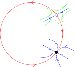
Figure 1: (color online) Schematic phase portrait below a SNIPER bifurcation. The full circle and the open circle mark the stable node and the saddle-point, respectively.

In this regime the system is very close to a saddle-node bifurcation on a limit cycle (saddle-node infinite period bifurcation, SNIPER). In HIZ06 a bifurcation analysis in the $(\sigma,U)$ plane was performed showing how SNIPER bifurcations govern the transition from stationary to moving field domains in the superlattice. In the vicinity of such a bifurcation the system is excitable LIN04 and therefore very sensitive to noise which is able to trigger front motion through the device. Moreover, the phenomenon of coherence resonance PIK97 was also confirmed in our model.

In this paper, we will study how time-delayed feedback acts on the system both in the presence and absence of noise. when prepared in the vicinity of a SNIPER bifurcation.

In the absence of both delay and noise the only stable attractor in phase space is the stable node. Regardless of the initial condition, all trajectories end there. In particular, when selecting the initial condition on one of the two unstable manifolds of the saddle-point, the system performs a long excursion along the invariant circle before ending in the stable node (Fig.1). This deterministic path is affected by the delay for given combinations of the two control parameters, $K$ and $\tau$. By keeping the delay $\tau$ fixed and considering different control amplitudes $K$ we track these orbits in phase space (Fig. 2). The top panel of Fig. 2(a) (K=0) shows a trajectory which closely follows the unstable manifold of the saddle-point (cross) and ends in the stable node (full circle), cf. blow-up in the middle panel. Note that in the chosen 2-dimensional projection of the N-dimensional phase space the invariant circle (saddle-node loop) is distorted to a figure-eight shape.

In Fig. 2(b), during the first few nanoseconds the systems acts as it would in the absence of delay, repelled by the saddle-point. Control is switched on at $t=\tau=2ns$ when the control force begins to act. The interval $[0,2ns]$ serves as initial condition of the delay equation. This becomes evident in a “twist” in the trajectory just before the orbit reaches the stable node (middle panel of Fig. 2(b)). For a moment it looks as if the system is attracted to the saddle-point instead of the node. This may be understood as follows: The control force shortly pulls the system off the phase space of the uncontrolled system pushing it towards the stable manifold of the saddle-point. At a critical value $K_{c}=0.0064375Vmm^{2}/A$, the system is indeed “swallowed” by the saddle and the trajectory closes in a homoclinic orbit.

In the top panel of Figs. 2(b) - 2(d) the trajectories for three values of $K$ approaching this critical value are shown.

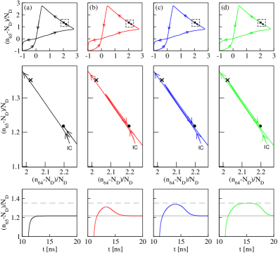
Figure 2: (color online) Top: Phase portrait in the $(n_{65},n_{64})$ plane for fixed $\tau=2ns$ and (a) $K=0$, (b) $0.006$, (c) $0.0064$ and (d) $0.006437Vmm^{2}/A$. Middle: Enlargement of corresponding phase portraits shown in upper plots. Cross marks the position of the saddle-point, full circle marks the position of the stable node and $IC$ is the initial condition, which is the same in all figures. Bottom: Corresponding electron density time series (only the part approaching asymptotically the stable node of $n_{65}$). Thick grey line denotes the value of the stable node and dashed grey line denotes that of the saddle-point. $U=2.99V$ and $\sigma=2.0821(\Omega m)^{-1}$.

Due to the high dimensionality of the system, which is blown up to infinity due to the delay, the above mechanism is not clearly demonstrated in a 2-dimensional projection in phase space. One must zoom in carefully in order to see the deviation from the deterministic path due to delay (middle panels of Fig. 2). This deviation is even better visible in the bottom panels of Fig. 2 where the final part of the electron density time series of $n_{65}$ is plotted. In (a) the deterministic trajectory is plotted and the thick grey solid and dashed lines mark the position of the stable node and the saddle-point, respectively. It is clear that, the closer one is to the homoclinic bifurcation (d), the closer to the saddle-point does the system reach and the longer the trajectory remains there, before ending up in the stable node.

Beyond the critical value of $K_{c}=0.00644Vmm^{2}/A$ the homoclinic orbit breaks and a limit cycle is born. In Figs. 3(a) - 3(c) the time series of the current density for three different values of $K$ above $K_{c}$ are shown. The period clearly decreases for increasing $K$. Plotting it as a function of the control strength we obtain Fig. 3 (d). The period $T$ shows a characteristic scaling law KUZ95 , $T\sim ln[K-K_{c}]$, shown in the inset. This law governs another type of global bifurcation, namely the homoclinic bifurcation. This delay-induced dynamics is in perfect agreement with a generic two-variable model for the SNIPER bifurcation, which also exhibits homoclinic bifurations of a limit cycle if delay is added HIZ07 . Here, however, we have a much more complex spatio-temporal system. The corresponding space-time plots are shown in Fig. 4. It is clear that accumulation and depletion fronts corresponding to dipole domains are created at the emitter (bottom), and move through the device. Due to the global voltage constraint, they interact with the additional accumulation front in the middle of the sample, thus forming a tripole oscillation AMA04 .

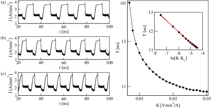
Figure 3: (a) Time series of the delay-induced limit cycle for fixed $\tau=2ns$ showing period lengthening as the homoclinic bifurcation is approached from above ($K>K_{c}$), for $K=0.0064379$, (b) $K=0.007$ and (c) $K=0.019Vmm^{2}/A$. (d) Period $T$ as a function of control amplitude $K$, and characteristic scaling law governing the homoclinic bifurcation shown in inset. $K_{c}=0.0064375Vmm^{2}/A$, $U=2.99V$, and $\sigma=2.0821(\Omega m)^{-1}$.

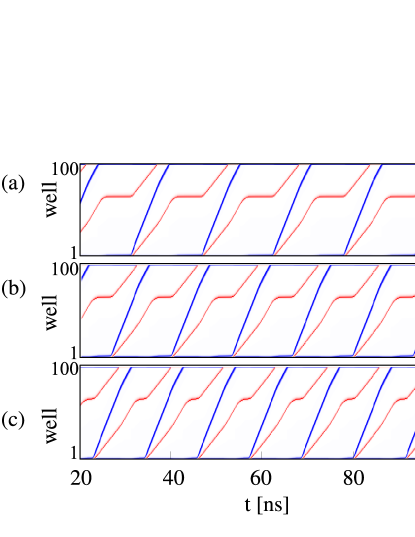
Figure 4: (color online). Delay-induced front motion: Space-time plots of the electron density for $K=0.0064379$, (b) $K=0.007$ and (c) $K=0.019Vmm^{2}/A$. Light (red) and dark (blue) shading corresponds to electron accumulation and depletion fronts, respectively. The emitter is at the bottom, the collector at the top. Parameters as in Fig. 3.

Following the homoclinic bifurcation in the $K$-$\tau$ plane we numerically obtain the regime where control induces limit cycle oscillations. The result is shown in Fig. 5.

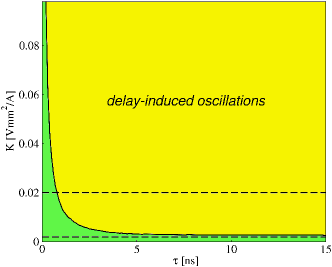
Figure 5: (color online) Bifurcation diagram in the $K$-$\tau$ plane below the SNIPER bifurcation in the superlattice. Yellow (light) area denotes the parameter regime for which delay-induced oscillation occur. In the green (dark) area there are no delay-induced bifurcations. The black line marks the delay-induced homoclinic bifurcation line. $U=2.99V$ and $\sigma=2.0821(\Omega m)^{-1}$.

Crossing the bifurcation line by increasing either $K$ or $\tau$, oscillations are born, whose period decreases with $K$ or $\tau$.

V Control of coherence resonance

In this section, Gaussian white noise is added according to Eqs. (1), (2). By considering two values of the control strength which lie inside or outside of the regime where delay induces a limit cycle (Fig.5)), we will study the effect of the time delay on noise-mediated and noise-induced oscillations, respectively.

The regularity or coherence of noisy oscillations can be quantified by various measures. Here we use (i) the correlation time STR63 :

$$t_{cor}=\frac{1}{\psi(0)}\int_{0}^{\infty}|\psi(s)|ds,$$ (8)

where $\psi(s)=\langle(J(t)-\langle J\rangle)(J(t+s)-\langle J\rangle)\rangle$ is the autocorrelation function of the current density signal $J(t)$, and (ii) the normalized fluctuation of pulse durations PIK97 :

$$R_{T}=\frac{\sqrt{\langle T^{2}\rangle-{\langle T\rangle}^{2}}}{\langle T\rangle},$$ (9)

typically used for excitable systems exhibiting oscillations in the form of spike trains with two distinct time scales. These time scales are the activation time, which is the time needed to excite the system from the stable fixed point and the excursion time which is the time needed to return from the excited state to the fixed point. The sum of these two times equals the pulse duration or period of the oscillation $T$, which denotes the time between two spikes and is also known as interspike interval.

By keeping the noise intensity fixed at $D=1.0As^{1/2}/m^{2}$ we first select a value $K=0.002Vmm^{2}/A$ outside the delay-induced limit cycle regime. This corresponds to the lower dashed horizontal line in Fig. 5. In the right panel of Fig. 6(a), the correlation time is plotted versus the time delay. It exhibits a slight modulation with a period close to the period of the noise-induced oscillations HIZ06 , $\langle T\rangle=14.5ns$ and reaches minimum values for $\tau=n\langle T\rangle,n\in\mathbb{N}$. Overall, however, it remains close to the control-free value, $t_{cor}=19.76ns$.

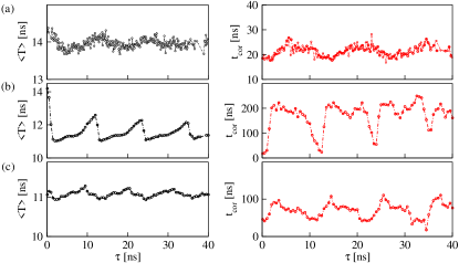
Figure 6: (color online) Mean interspike interval $\langle T\rangle$ (left) and correlation time $t_{cor}$ (right) in dependence on the time delay $\tau$. (a) Control strength $K=0.002Vmm^{2}/A$ and noise intensity $D=1.0As^{1/2}/m^{2}$, (b) $K=0.02Vmm^{2}/A$ and $D=1.0As^{1/2}/m^{2}$ and (c) $K=0.02Vmm^{2}/A$ and $D=2.5As^{1/2}/m^{2}$. Averages over 30 time series realizations of length $T=1600ns$ have been used for the calculation of $t_{cor}$ and averages over 1000 periods for $\langle T\rangle$. $U=2.99V$ and $\sigma=2.0821(\Omega m)^{-1}$.

At $K=0.02Vmm^{2}/A$ inside the delay-induced limit cycle regime (upper dashed line in Fig. 5), this modulation is much stronger and has a period close to the delay-induced period ($T=11ns$, see Fig. 3(d)). In addition, one can better distinguish between non-optimal and optimal values of $\tau$ at which the correlation time attains maximum values. This is shown in the right panel of Fig. 6 (b). For a higher noise intensity (Fig. 6 (c), right panel) the effect is similar but weaker.

Next we are interested in how the time scales are affected by the delay. We express the time scales through the mean interspike interval $\langle T\rangle$ and look at its dependence upon the time delay $\tau$ for a fixed value of the noise intensity, $D=1.0As^{1/2}/m^{2}$, and control strength $K=0.002Vmm^{2}/A$, chosen outside of the delay-induced oscillations regime (lower dashed line in Fig. 5). As shown in the left panel of Fig. 6 (a), $\langle T\rangle$ is slightly modulated due to the delay with a period close to the noise-induced mean period ($\langle T\rangle\approx 14.5ns$) HIZ06 .

In the left panel of Fig. 6 (b) a value of $K$ inside the delay-induced oscillations regime is used, $K=0.02Vmm^{2}/A$ (upper dashed line in Fig. 5). For $\tau=0$, the mean interspike interval is equal to the noise-induced period, $\langle T\rangle\approx 14.5ns$ HIZ06 . As the time delay increases, and the delay-induced bifurcation line is crossed, $\langle T\rangle$ sharply drops to the value of $11ns$ which corresponds to the period induced by the delay (see Fig. 3(d)). By further increase of $\tau$, $\langle T\rangle$ rises a little above $12ns$. Then, for $\tau=11ns$ the mean interspike interval decreases again and the same scenario is repeated with a modulation period very close to the delay-induced period.

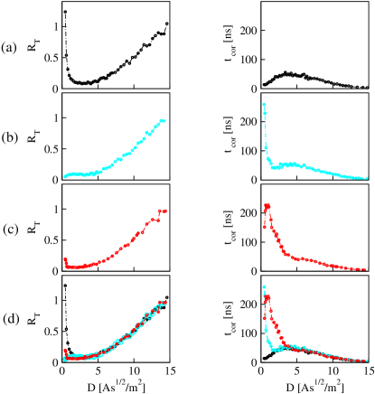
Figure 7: (color online) Correlation time (right) and normalized fluctuation of pulse durations (left) as a function of the noise intensity for (a) $K=0$, (b) $(K,\tau)=(0.02Vmm^{2}/A,11ns)$ and (c) $(K,\tau)=(0.02Vmm^{2}/A,14.5ns)$. All three curves plotted together in (d). Averages over 30 time series realizations of length $T=1600ns$ have been used for the calculation of $t_{cor}$ and averages over 1000 periods for $R_{T}$. $U=2.99V$ and $\sigma=2.0821(\Omega m)^{-1}$.

There is some resemblance to the piecewise linear dependence of $\langle T\rangle$ upon $\tau$ reported in other excitable systems: The FitzHugh-Nagumo model in JAN03 ; BAL04 ; PRA07 and the Oregonator model of the Belousov-Zhabotinsky reaction (under correlated noise and nonlinear delayed feedback) in BAL06 which, like our system, is also spatially extended. The difference to our present analysis is that in those models the case of a delay-induced limit cycle was excluded. An explanation for the entrainment of the time scales by the delayed feedback in case of systems below a Hopf bifurcation JAN03 ; BAL04 ; POM05a ; STE05a was given on the basis of a linear stability analysis. It was shown that the basic period is proportional to the inverse of the imaginary part of the eigenvalue of the fixed point which itself depends linearly upon $\tau$, for large time delays. The effect of noise and delay in excitable systems was also studied analytically in PRA07 ; POT08 based on waiting time distributions and renewal theory.

Finally we look into the dependence of the correlation time $t_{cor}$ and the normalized fluctuation of the interspike intervals $R_{T}$ on the noise intensity. We keep the control strength fixed to the value corresponding to Fig. 6(b) (right panel), from which we also select an optimal and a non-optimal value of the time delay and compare the results to the uncontrolled system. In the left and right panel of Fig. 7, $R_{T}$ and $t_{cor}$ are plotted, respectively. The case $K=0$ is shown in Fig. 7(a) for direct comparison. Coherence resonance shows up as a minimum of $R_{T}$ and a maximum of $t_{cor}$, respectively. For both non-optimal (Fig. 7(b)) and optimal $\tau$ (Fig. 7(c)), there is an enhancement in the coherence at low noise intensity. Correlation times attain much higher values than those of the uncontrolled system, especially at low noise level. Similarly, the interspike interval fluctuation $R_{T}$ is much smaller. In addition, for non-optimal delay time $\tau\approx 11ns$, the effect of coherence resonance is suppressed (Fig. 7(b)). The correlation time still shows a small local maximum exactly where the uncontrolled system does, but for small noise intensities the correlation time dramatically increases in a monotonic way to much larger values of $t_{cor}$. On the other hand, for optimal $\tau\approx 14.5ns$ (Fig. 7(c)), coherence resonance is maintained and both $t_{cor}$ and $R_{T}$ show a maximum and minimum, respectively, but at a much lower noise intensity than in the free system. The comparison between all three cases is better visible in Fig. 7(d) where the three curves are plotted together.

VI Conclusions

We have shown that by applying a time-delayed feedback force to a semiconductor superlattice stationary field domains (bounded by charge accumulation and depletion fronts) can be transformed into travelling domains in a homoclinic bifurcation of a limit cycle if the system is prepared below a saddle-node infinite period SNIPER bifurcation. With the addition of Gaussian white noise, control results in a modulation of both the coherence and time scales of the system with the time delay. The periodicity of this modulation is determined by the competition between the different time scales imposed by noise and control and their dependence on the noise intensity and time-delay, respectively. We distinguish between optimal and non-optimal time delays at which the coherenc resonance effect is enhanced or destroyed, respectively. In both cases the correlation times of stochastic domain motion are dramatically increased at low noise intensities.

VII Acknowledgements

This work was supported by DFG in the framework of Sfb 555.

References

- (1) Handbook of Chaos Control, edited by E. Schöll and H. G. Schuster (Wiley-VCH, Weinheim, 2008), second completely revised and enlarged edition.
- (2) G. Hu, T. Ditzinger, C. Z. Ning, and H. Haken, Phys. Rev. Lett. 71, 807 (1993).
- (3) A. Pikovsky and J. Kurths, Phys. Rev. Lett. 78, 775 (1997).
- (4) P. Tass, Phys. Rev. E 66, 036226 (2002).
- (5) D. Goldobin, M. G. Rosenblum, and A. Pikovsky, Phys. Rev. E 67, 061119 (2003).
- (6) N. B. Janson, A. G. Balanov, and E. Schöll, Phys. Rev. Lett. 93, 010601 (2004).
- (7) A. G. Balanov, N. B. Janson, and E. Schöll, Physica D 199, 1 (2004).
- (8) J. Pomplun, A. Amann, and E. Schöll, Europhys. Lett. 71, 366 (2005).
- (9) B. Hauschildt, N. B. Janson, A. G. Balanov, and E. Schöll, Phys. Rev. E 74, 051906 (2006).
- (10) T. Prager, H. P. Lerch, L. Schimansky-Geier, and E. Schöll, J. Phys. A 40, 11045 (2007).
- (11) A. Pototsky and N. B. Janson, Phys. Rev. E 76, 056208 (2007).
- (12) A. Pototsky and N. B. Janson, Phys. Rev. E 77, 031113 (2008).
- (13) J. Hizanidis, A. G. Balanov, A. Amann, and E. Schöll, Int. J. Bifur. Chaos 16, 1701 (2006).
- (14) G. Stegemann, A. G. Balanov, and E. Schöll, Phys. Rev. E 73, 016203 (2006).
- (15) A. G. Balanov, V. Beato, N. B. Janson, H. Engel, and E. Schöll, Phys. Rev. E 74, 016214 (2006).
- (16) J. Hizanidis, A. G. Balanov, A. Amann, and E. Schöll, Phys. Rev. Lett. 96, 244104 (2006).
- (17) E. Schöll, Nonlinear spatio-temporal dynamics and chaos in semiconductors (Cambridge University Press, Cambridge, 2001).
- (18) J. Kastrup, R. Klann, H. T. Grahn, K. Ploog, L. L. Bonilla, J. Galán, M. Kindelan, M. Moscoso, and R. Merlin, Phys. Rev. B 52, 13761 (1995).
- (19) K. Hofbeck, J. Grenzer, E. Schomburg, A. A. Ignatov, K. F. Renk, D. G. Pavel’ev, Y. Koschurinov, B. Melzer, S. Ivanov, S. Schaposchnikov, and P. S. Kop’ev, Phys. Lett. A 218, 349 (1996).
- (20) E. Schomburg, R. Scheuerer, S. Brandl, K. F. Renk, D. G. Pavel’ev, Y. Koschurinov, V. M. Ustinov, A. E. Zhukov, A. R. Kovsh, and P. S. Kop’ev, Electronics Letters 35, 1491 (1999).
- (21) A. Wacker, Phys. Rep. 357, 1 (2002).
- (22) A. Amann and E. Schöll, J. Stat. Phys. 119, 1069 (2005).
- (23) Microscopic parameters: energy levels and , scattering width , transition matrix elements , and AMA04 .
- (24) M. Patra, G. Schwarz, and E. Schöll, Phys. Rev. B 57, 1824 (1998).
- (25) A. Amann, K. Peters, U. Parlitz, A. Wacker, and E. Schöll, Phys. Rev. Lett. 91, 066601 (2003).
- (26) H. Xu and S. W. Teitsworth, Phys. Rev. B 76, 235302 (2007).
- (27) K. Pyragas, Phys. Lett. A 170, 421 (1992).
- (28) A. Ahlborn and U. Parlitz, Phys. Rev. Lett. 93, 264101 (2004).
- (29) P. Hövel and E. Schöll, Phys. Rev. E 72, 046203 (2005).
- (30) J. E. S. Socolar, D. W. Sukow, and D. J. Gauthier, Phys. Rev. E 50, 3245 (1994).
- (31) O. Beck, A. Amann, E. Schöll, J. E. S. Socolar, and W. Just, Phys. Rev. E 66, 016213 (2002).
- (32) J. Unkelbach, A. Amann, W. Just, and E. Schöll, Phys. Rev. E 68, 026204 (2003).
- (33) J. Schlesner, A. Amann, N. B. Janson, W. Just, and E. Schöll, Phys. Rev. E 68, 066208 (2003).
- (34) T. Dahms, P. Hövel, and E. Schöll, Phys. Rev. E 76, 056201 (2007).
- (35) J. Pomplun, A. G. Balanov, and E. Schöll, Phys. Rev. E 75, 040101(R) (2007).
- (36) E. Schöll, N. Majer, and G. Stegemann, phys. stat. sol. (c) 5, 194 (2008).
- (37) T. Heil, I. Fischer, W. Elsäßer, and A. Gavrielides, Phys. Rev. Lett. 87, 243901 (2001).
- (38) S. Schikora, P. Hövel, H. J. Wünsche, E. Schöll, and F. Henneberger, Phys. Rev. Lett. 97, 213902 (2006).
- (39) V. Flunkert and E. Schöll, Phys. Rev. E 76, 066202 (2007).
- (40) M. A. Dahlem, F. M. Schneider, and E. Schöll, Chaos 18, 026110 (2008).
- (41) B. Lindner, J. García-Ojalvo, A. Neiman, and L. Schimansky-Geier, Phys. Rep. 392, 321 (2004).
- (42) Y. A. Kuznetsov, Elements of Applied Bifurcation Theory (Springer, New York, 1995).
- (43) J. Hizanidis, R. Aust, and E. Schöll, Int. J. Bifur. Chaos (2008), in print (arXiv:nlin/0702002v2).
- (44) R. L. Stratonovich, Topics in the Theory of Random Noise (Gordon and Breach, New York, 1963), Vol. 1.