Constraints on core-collapse supernova progenitors from correlations with H$\alpha$ emission

Abstract

We present observational constraints on the nature of the different core-collapse supernova types through an investigation of the association of their explosion sites with recent star formation, as traced by H$\alpha$+[Nii] line emission. We discuss results on the analysed data of the positions of 168 core-collapse supernovae with respect to the H$\alpha$ emission within their host galaxies.
From our analysis we find that overall the type II progenitor population does not trace the underlying star formation. Our results are consistent with a significant fraction of SNII arising from progenitor stars of less than 10${\rm\ M}_{\odot}$. We find that the supernovae of type Ib show a higher degree of association with HII regions than those of type II (without accurately tracing the emission), while the type Ic population accurately traces the H$\alpha$ emission. This implies that the main core-collapse supernova types form a sequence of increasing progenitor mass, from the type II, to Ib and finally Ic. We find that the type IIn sub-class display a similar degree of association with the line emission to the overall SNII population, implying that at least the majority of these SNe do not arise from the most massive stars. We also find that the small number of SN ‘impostors’ within our sample do not trace the star formation of their host galaxies, a result that would not be expected if these events arise from massive Luminous Blue Variable star progenitors.

1 Introduction

Despite years of observational and theoretical research on the nature of supernova (SN) explosions and the properties of their progenitors there remain substantial gaps in our knowledge of all SN types. Although there are many different theoretical predictions as to the nature of SN progenitors, the observational evidence to discriminate between various progenitor scenarios remains sparse. SNe can be split into two theoretical classes; SNIa which are thought to arise from the thermonuclear explosion of an accreting white dwarf, and core-collapse (CC) SNe which are believed to signal the collapse of the cores of massive stars at the end points in their stellar evolution.
Results from the first paper in this series (James & Anderson 2006, JA06 henceforth) suggested that the SNIb/c arise from higher mass progenitors than SNII (albeit with small statistics; only 8 SNIb/c). We test these initial results with an increased sample size enabling us to distinguish between the various CC sub-types, and present results from a combined sample of 100 SNII (that can be further separated into 37 IIP, 8 IIL, 4 IIb, 12 IIn), 62 SNIb/c (22 Ib, 34 Ic and 6 that only have Ib/c classification), and 6 SN ‘impostors’. We will present results and discussion of SNIa within the context of the methods used in this paper elsewhere. We will also present further research on the radial positions of SNe within galaxies, and on correlations between CC SN type and local metallicity in future publications. Here we concentrate on results on the progenitor masses of the different CC SNe.

1.1 Core-collapse supernovae

CC SNe are thought to be the final stage in the stellar evolution of stars with initial masses $>$8-10${\rm\ M}_{\odot}$, when fusion ceases in the cores of their progenitors and they can no longer support themselves against gravitational collapse. The different types of CC SNe are classified according to the presence/absence of spectral lines in their early time spectra, plus the shape of their light curves. The first major classification comes from the presence of strong hydrogen (H) emission in the SNII. SNIb and Ic lack any detectable H emission, while the SNIc also lack the helium lines seen in SNIb. SNII can also be separated in various sub-types. SNIIP and IIL are classified in terms of the decline shape of their light curves (Barbon et al. 1979; plateau in the former and linear in the latter), thought to indicate different masses of their H envelopes prior to SN, while SNIIn show narrow emission lines within their spectra (Schlegel, 1990), thought to arise from interaction of the SN ejecta with a slow-moving circumstellar medium (e.g. Chugai & Danziger 1994). SNIIb are thought to be intermediate objects between the SNII and Ib as at early times their spectra are similar to SNII (prominent H lines), while at later times they appear similar to SNIb (Filippenko et al. 1993).
Strong evidence has been presented to support the belief that SNII and SNIb/c arise from massive progenitors, through their absence in early type galaxies (van den Bergh et al., 2002), and the direct detection of a small sample of progenitors on pre-explosion images (Smartt et al. 2004; Maund et al. 2005; Hendry et al. 2006; Li et al. 2006; Gal-Yam et al. 2007; Li et al. 2007; Crockett et al. 2008). However, it is unclear how differences in the nature of their progenitors produce the different SNe we see. It is clear that there must be some process by which the progenitors of the different SNe lose part (or almost all in the case of SNIb and Ic) of their envelopes prior to explosion. The differences in efficiency of this mass loss process could be dependent primarily on progenitor mass, with higher mass progenitors having higher mass loss rates due to stronger stellar winds, and losing more of their envelopes. In this picture a sequence of SNe types emerges from SNIIP and IIL to SNIIb, SNIb and finally Ic having successively higher initial masses. There are also other factors that probably play an important role. Initial chemical abundance will also affect the progenitor mass loss, with higher metallicity producing stronger radiatively driven winds (e.g. Puls et al. 1996; Kudritzki & Puls 2000; Mokiem et al. 2007). It has also been proposed (Podsiadlowski et al., 1992) that massive binaries could produce a significant fraction of CC SNe, with mass transfer ejecting matter and leading to some of the various CC sub-types.
Since the theoretical separation of SNe into two distinct explosion classes by Hoyle & Fowler (1960), there have been many predictions as to how the different CC SN types emerge from different progenitors. There are two main theoretical routes to achieving the observed different SN types. The first attempts to describe the full range of SNe from a single star progenitor scenario. Heger et al. (2003) and Eldridge & Tout (2004) produced SN progenitor maps showing how variations in initial mass and metallicity produced the different CC SN types. These models both predict that single stars of up to $\sim$25-30${\rm\ M}_{\odot}$ will produce SNIIP, with stars of slightly higher mass producing SNIIL and IIb, and those of $>$30${\rm\ M}_{\odot}$ ending their lives as SNIb/c (both authors also predict that these initial mass ranges will shift to higher values with decreasing metallicity). In both of these models no attempt was made to differentiate between the SNIb and the SNIc, but one would presume that within this single star scenario SNIc would arise from higher mass progenitors than the SNIb as they have lost even more of their stellar envelopes. Alternatively it could be that massive binaries produce the majority of CC SNe other than SNIIP (with these SNe still arising from single star progenitors). The initial mass of the stars producing SNIb/c, SNIIL and SNIIb would then be similar to those of SNIIP (12-20${\rm\ M}_{\odot}$, e.g. Shigeyama et al. 1990) but would arise from binary evolutionary processes. There is also a growing number of SNe that show evidence of binarity (e.g. SN 1987A; Podsiadlowski et al. 1990 and SN 1993J; Nomoto et al. 1993; Podsiadlowski et al. 1993; Maund et al. 2004). Recent comparisons of the observed ratio of SNIb/c rates to those of SNII also argue that binaries are playing the dominant role in producing SNIb/c (Kobulnicky & Fryer, 2007), while Eldridge et al. (2008) predict a SNIb/c rate produced by a combination of single and binary progenitors that best produces the observed SN rate. Again one should note that these binary models group SNIb and Ic together and do not attempt to predict what differences in progenitor produce these two types.
Given the different predictions for the origin of the CC SN types described above, observations are needed to discriminate between these models and thus firmly tie down the progenitors of the different SN types. However, apart from a small number of direct detections of progenitors (Smartt et al. 2004; Maund et al. 2005; Hendry et al. 2006; Li et al. 2006; Gal-Yam et al. 2007; Li et al. 2007; Crockett et al. 2008) this observational evidence remains sparse. Therefore here we present results to test the above predictions and constrain differences in progenitor mass of the different CC SN sub-types by investigating the nature of their parent stellar populations within host galaxies.

1.2 Progenitor constraints from parent stellar populations

The most obvious way to determine the nature of SN progenitors is to investigate the properties of their stars on pre-explosion images. This has had some success although it is only possible for events in very nearby galaxies and therefore the statistics remain low. Another way is to investigate how the rates of the various SN types vary with different parameters, such as redshift or host galaxy properties. Our approach is intermediate to these methods as we attempt to constrain the nature of SN progenitors through investigating the environments and stellar populations at the positions of historical SNe. Here we concentrate on the association of the different CC SNe types with recent star formation (SF) as traced by H$\alpha$ emission.
Kennicutt (1998) states in a review paper on H$\alpha$ imaging techniques that: “only stars with masses $>$10${\rm\ M}_{\odot}$ and lifetimes of $<$20 Myr contribute significantly to the ionising flux”. Thus, if our understanding of this line emission is correct, we can use this assumption as a starting point to constrain the relative stellar lifetimes and therefore the relative masses of the various SN progenitors, through investigating how accurately the different SN types trace the emission. In JA06 we presented a statistic to quantitatively measure the association of individual SNe with the H$\alpha$ emission of their host galaxies, and presented results from an initial galaxy sample (H$\alpha$GS, discussed in §2). It was found that overall the SNII progenitor population did not trace the underlying SF of their host galaxies, with a significant fraction lying on regions of low or zero emission line flux which were ascribed to a ‘Runaway’ fraction of progenitor stars (however, this assumed that SNII arise from progenitors of $>$10${\rm\ M}_{\odot}$). The SNIb/c did appear to follow the emission implying that these progenitors come from higher mass stars than the SNII, although the statistics on this class were small (only 8 SNe for SNIb and Ic combined). This SN/galaxy sample has now been significantly increased, enabling the full parameter space of CC SN progenitors to be investigated and results from this increased sample are presented here.
The paper is arranged as follows: in the next section we present the data and discuss the reduction techniques employed, in §3 we summarise the statistic introduced in JA06 and used throughout this paper, in §4 we present the results for the different CC SN types, in §5 we discuss possible explanations for these results and their implications for the relative masses of the SN progenitors, and finally in §6 we draw our conclusions.

2 Data

The initial galaxy sample that formed the data set for JA06 was the H$\alpha$ Galaxy Survey (H$\alpha$GS). This survey was a study of the SF properties of the local Universe using H$\alpha$ imaging of a representative sample of nearby galaxies, details of which can be found in James et al. (2004). 63 SNe (of all types, including SNIa) were found to have occurred in the 327 H$\alpha$GS galaxies through searching the International Astronomical Union (IAU) database .
Through three observing runs on the Isaac Newton Telescope (INT) and an on-going time allocation with the Liverpool Telescope (LT) we have now obtained H$\alpha$ imaging for the host galaxies of 133 additional CC SNe, the analysis of which is presented here. The LT is a fully robotic 2m telescope operated remotely by Liverpool John Moores University. To obtain our imaging we used RATcam together with the narrow H$\alpha$ and the broad-band Sloan r’ filters. Images were binned 2$\times$2 to give us 0.278^′′ size pixels, and the width of the H$\alpha$ filter enabled us to image target galaxies out to $\sim$2400 kms^-1. The INT observations used the Wide Field Camera (WFC) together with the Harris R-band filter, plus the rest frame narrow H$\alpha$ (filter 197) and the redshifted H$\alpha$ (227) filters enabling us to image host galaxies out to $\sim$6000 kms^-1. During our 2005 INT observing run we also used the SII filter (212) as a redshifted H$\alpha$ filter and imaged 12 SN hosting galaxies at distances of $\sim$7500 kms^-1. The pixel scale on all INT images is 0.333^′′ per pixel and with both the LT and INT our exposure times were $\sim$800 sec in H$\alpha$ and $\sim$300 sec in R.
These additional SNe/galaxies were chosen from the Padova-Asiago SN catalogue, as specific CC SN types were more complete for the listed SNe. At a later date all SN type classifications taken from the Padova-Asiago catalogue were checked through a thorough search of the literature and IAU circulars, as classifications can often change after the initial discovery and therefore those in the catalogue may not be completely accurate. The full list of SN types is given in Appendix B, where references are given if classifications were changed from those in the above catalogue. The main discrepancies were the classification of the so called SN ‘impostors’ as SNIIn in the Padova-Asiago catalogue. These are transient objects that are believed to be the outbursts from very massive Luminous Blue Variable stars (LBVs), which do not fully destroy the progenitor star and are therefore not classed as true SNe (e.g. van Dyk et al. 2000; Maund et al. 2006). Six such objects were found in our sample, and the results on these ‘impostors’ are presented and discussed separately in the following sections.
The distance limit for our sample (mainly set from the available H$\alpha$ filters during observing runs) enables us to resolve the stellar population close to the SN position, and we also exclude edge on galaxies because of extinction effects and increased projection uncertainties. We do not include results on SNe where images were obtained within 18 months for SNII and a year for SNIb/c after the catalogued explosion epoch. This is to ensure that our images are not contaminated with residual SN light and that the H$\alpha$ emission that we detect is due to the underlying HII regions and not associated with the SNe themselves. Through the above telescope time allocations we have therefore obtained data on host galaxies of almost all discovered CC SNe (that have been classified IIP, IIL, IIb, IIn, Ib, and Ic) that meet our selection criteria and were observable within the H$\alpha$ filters of the two telescopes.
There are obvious biases within a set of data chosen in the above way. As we use any discovered SNe for our sample, the various different biases in the different SN surveys that discovered them mean that the galaxy/SN sample is by no means representative of the overall SN populations. Bright, well studied galaxies will be over represented, as will brighter SNe events that are more easily detectable. However, firstly we are not analysing the overall host galaxy properties (as we will show when discussing the statistics we use in §3), but are analysing where within the distribution of stellar populations of the host galaxy the SNe are occurring. Secondly, the small number of CC sub-types that are discovered means that no individual survey can currently manage to analyse the properties of their host galaxies or parent stellar populations in any statistically significant way (most statistical observational studies do not even attempt to separate the Ib and Ic SN types). Taking our approach enables us to make statistical constraints on all the major CC SN sub-types. The results that are presented in this paper are on the analysis of the parent stellar populations of 100 SNII, of which 37 are IIP, 8 IIL, 4 IIb and 12 IIn, 6 SN ‘impostors’, plus 22 Ib, 34 Ic and 6 that only have Ib/c as their classification, from both the initial H$\alpha$GS sample and our additional data described above.

2.1 Data reduction and astrometric methods

For each SN host galaxy we obtained H$\alpha$+[Nii] narrow band imaging, plus R- or r’-band imaging used for continuum subtraction. Standard data reduction (flat-fields, bias subtraction etc) were achieved through the automated pipeline of the LT (Steele et al., 2004), and the INT data were processed through the INT Wide Field Camera (WFC), Cambridge Astronomical Survey Unit (CASU) reduction pipeline. Continuum subtraction was then achieved by scaling the broad-band image fluxes to those of the H$\alpha$ images using stars matched on each image, and subtracting the broad-band image from the H$\alpha$ images. Our reduction made use of various Starlink packages.
The next process was to obtain accurate positions for the sites of our SNe on their host galaxy images. This astrometric calibration was achieved by transferring the accurate astrometry of XDSS second generation Palomar Sky Survey images, onto matching galaxy images in our sample (the full process is described in JA06). In nearly all cases astrometric calibration was achieved with fit residuals of $<$0.2^′′. With accurate positions obtained for the SNe sites we could now analyse to what degree the different SNe were associated with the distribution of H$\alpha$ emission within their host galaxies.
In figures 1 and 2 we show two examples of H$\alpha$ images of the host galaxies of SNe from our sample, with SN positions derived from the above astrometric calibration. We intend to present all our H$\alpha$ and R-band imaging of SN host galaxies in a future publication (Ivory et al. 2008, in prep), where we will release all of our data for public use along with host galaxy derived characteristics such as SF rates and H$\alpha$ equivalent widths.

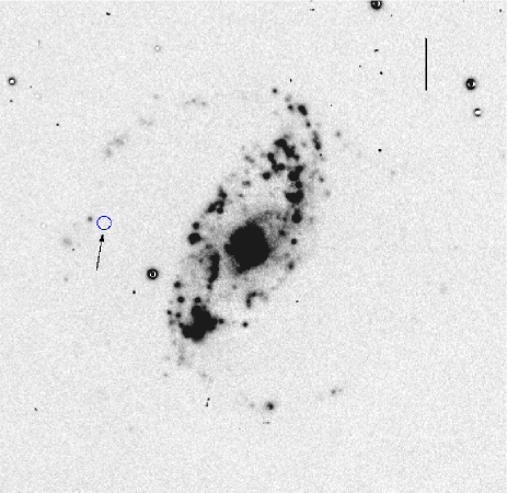
Figure 1: An example negative continuum subtracted H$\alpha$ image from our data (image taken with the WFC on the INT); SN 2001ac (SN ‘impostor’) (position indicated by circle/arrow), within the host galaxy NGC 3504. The scale bar is 20^′′. The NCR value for this SN is 0.000.

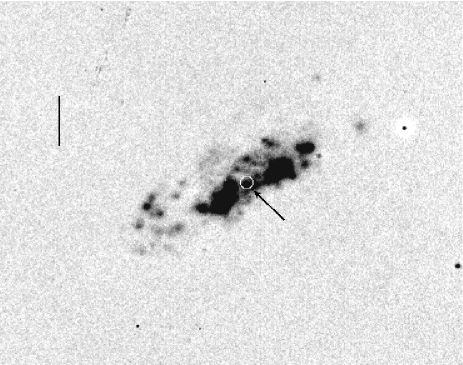
Figure 2: Another example negative continuum subtracted H$\alpha$ image (WFC, INT); SN 2004bm (Ic) (position indicated by circle/arrow), within the host galaxy NGC 3437. The scale bar is 20^′′. The NCR value for this SN is 0.704.

3 Pixel statistics

Previous works investigating the association of SNe with HII regions within host galaxies (e.g. Bartunov et al. 1994; van Dyk et al. 1996) have generally used some measure of the distance to the nearest bright HII region to quantify the association of each individual SN to the high mass SF within their host galaxies. However, this brings various problems when defining the nearest bright HII region and therefore the distance to measure. In JA06 we presented a quantitative statistic that reduced any ambiguity in the measurements of each SN, by analysing where the count of the SN hosting pixel falls within the overall distribution of H$\alpha$ pixel values of the galaxy. The exact details of how this statistic is formed can be found in JA06, and here we summarise this process and the main points on how this can be used in analysing the associations of the different SN types to the emission.
The pixels in the continuum subtracted H$\alpha$ images were first binned 3$\times$3 to reduce the pixel-to-pixel noise level and enable us to determine the SN-containing pixel with a degree of certainty. The pixels were then sorted into increasing pixel count. The cumulative distribution of these values was then formed and normalised, with negative values set to zero, giving a normalised cumulative rank pixel value function (NCR henceforth) running from 0 to 1, with one entry for each pixel on the host galaxy image. Within this distribution therefore, values of 0 correspond to zero emission line flux or sky values, whereas a value of 1 corresponds to the centre of the brightest HII region on the image. Figures 1 and 2 illustrate the use of this statistic, with the SN ‘impostor’ 2001ac falling away from any detected H$\alpha$ emission in Fig. 1 and therefore having an NCR value of 0.000, whereas in Fig. 2 the SNIc 2004bm falls on a bright HII region and therefore has a high NCR value of 0.704.
When we form the NCR it is found that the majority of values lying above the sky level within this distribution are small and individually contribute little to the overall flux, but by force of numbers they do contribute a significant amount to the underlying SF. Alongside this, there will be relatively few NCR values close to 1, but those that are will individually make a significant contribution to the overall flux. Thus the distribution is formed so that if a SN progenitor population is drawn from the same stellar population that produces the H$\alpha$ flux, one would expect a mean NCR value for that SN type of 0.5 and a flat distribution. This is therefore the initial hypothesis that we work from, that if the progenitors of CC SNe trace the same high mass SF as does H$\alpha$ emission, we expect their NCR values to form a flat distribution. We can then investigate whether there are any differences in the mean NCR values and distributions of the different CC SN sub-types and what this may imply for differences in the relative lifetimes and masses of their progenitors.
A full discussion of the errors associated with this statistic was presented in JA06, therefore here we will summarise the main errors; those presented with the results are the statistical errors found on the various distributions. The most obvious error is that associated with the determination of the SN containing pixel. This was investigated by determining the NCR value of each SN for a 3$\times$3 pixel box centred on the SN pixel (meaning that after already binning 3$\times$3 we sample regions $\sim$2.5^′′ and 3^′′ on the LT and INT images respectively). A comparison was then made of the median NCR value of the box with the SN pixel. This was repeated for the new sample where we find the size of the errors to be consistent with those from JA06, and there are in general no significant differences between the SN pixel NCR values and those of the median value of the surrounding pixels. For the overall SNII NCR distribution we find a mean difference of 0.027 between the NCR value of the SN pixel and the median pixel. The rms difference in NCR value is 0.163 where, as in JA06 this is dominated by around five cases where there is a significant difference between the values. However, overall the NCR analysis seems to give results which are robust to positional errors of 1-2^′′. In JA06 possible errors due to the adopted sky level were investigated but these were found to be insignificant. Finally a Monte Carlo analysis was performed on the effects of pixel-to-pixel noise on the NCR value. Again this effect was found to be small, with errors appearing to be random and producing no tendency to bias the results in any particular direction. We will now present the results formed from using the above described statistic on the various CC SN types.

4 Results

4.1 SNII

Figure 3 shows the overall distribution of NCR values for the 100 SNII our sample. It is immediately clear that the positions of SNII do not follow the overall distribution of SF as traced by the H$\alpha$ line emission, confirming the result of JA06. In fact there is an excess of $\sim$35% of SNII that fall on sites of little or zero H$\alpha$ flux compared to what would be expected if these SNe followed the distribution of H$\alpha$ emission. The probability of the SNII progenitor population being drawn from a flat distribution (i.e. following the line emission), calculated using a Kolmogorov-Smirnov (KS) test is $<$1%. Overall the mean NCR value for SNII is 0.252 with a standard error on the mean of 0.027. We will now present the results obtained when separating the SNII into their various sub-types. It should be noted here that $\sim$40% of our type II SNe do not have designated sub-types and are only classified as SNII.

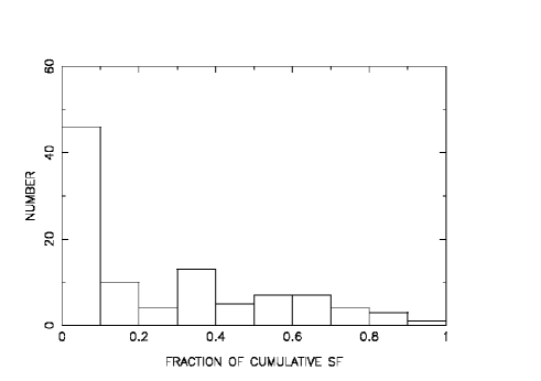
Figure 3: Histogram of the NCR values of the SN-containing pixels within the cumulative H$\alpha$ flux distribution for the 100 SNII

4.1.1 SNIIP

SNIIP are the most abundant SNII sub-type observed and therefore it is not surprising that these are the most abundant of those with sub-type classification in our sample. It is also to be expected that their distribution of NCR values follows that of the overall SNII population as can be seen when comparing Figs. 3 and 4, with a KS test showing that the two distributions (SNe classified as IIP removed from the overall II distribution) are formally consistent with each other. Again, if one assumes that the majority of those unclassified SNII will be of type IIP (i.e. if sufficient data were available on their light curves etc), this is to be expected. The mean NCR value for the SNIIP population is 0.263 (0.048).

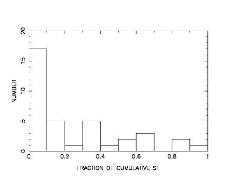
Figure 4: Histogram of the NCR values of the SN-containing pixels within the cumulative H$\alpha$ flux distribution for the 37 SNIIP

4.1.2 SNIIL

The 8 SNIIL population have a mean NCR value of 0.255 (0.112) and seem to follow the same distribution as the overall SNII population.

4.1.3 SNIIb

The 4 SNIIb have a mean NCR value of 0.460 (0.162), higher than that of the overall SNII population. To measure the significance of this difference we used a Monte Carlo analysis. Removing the SNIIb from the distribution of SNII NCR values we calculated the fraction of times that a mean NCR value of $\geq$0.460 (SNIIb mean value) was produced when four values were drawn at random from the overall SNII distribution. We found that there is only a $\sim$6% chance that the SNIIb parent population is drawn from the same distribution as that of the rest of the SNII.

4.1.4 SNIIn

Figure 5 shows the distribution of the NCR values for the 12 SNIIn. The mean NCR value for this SN type is 0.256 (0.088), and these SNe seem to follow the same stellar population as that of the overall SNII population. Using a KS test we find that there is only $\sim$1% chance that these SNe are drawn from a flat distribution (i.e. following the distribution of H$\alpha$ emission).

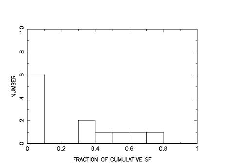
Figure 5: Histogram of the NCR values of the SN-containing pixels within the cumulative H$\alpha$ flux distribution of the 12 SNIIn

4.2 SNIb/c

The distribution of NCR values for the 62 SNIb/c is plotted in Fig. 6. Overall the mean NCR value of these SNe is 0.421 (0.040) and these SNe are formally consistent with being drawn from the same distribution as that traced by the H$\alpha$ emission, while there is $<$1% chance that they arise from the same parent distribution as the SNII. We have presented the results for this overall SNIb/c group to make comparisons to the overall SNII progenitor population (as is often quoted elsewhere), however it is clear that in fact the results for each separate group (Ib, Ic) differ as we will now discuss.

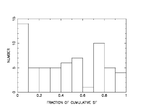
Figure 6: Histogram of the NCR values of the SN-containing pixels within the cumulative H$\alpha$ flux distribution for the 62 SNIb/c

4.2.1 SNIb

Figure 7 shows the distribution of NCR values for the SNIb population; this SNe type has a mean NCR value of 0.367 (0.063). The probability of this SN class being drawn from a flat distribution is $>$10%. We compare this population with that of the SNII and find that although the mean NCR value for the SNIb is higher than that of the SNII, using a KS test they are formally consistent with being drawn from the same progenitor population ($>$10% chance that they arise from the same distribution).

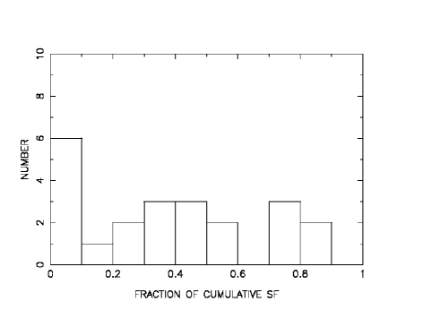
Figure 7: Histogram of the NCR values of the SN-containing pixels within the cumulative H$\alpha$ flux distribution of the 21 SNIb

4.2.2 SNIc

The distribution of NCR values for the SNIc is shown in Fig. 8. This is the SN type that shows the highest degree of association to the recent SF in host galaxies, as traced by H$\alpha$ emission and the population has a mean NCR of 0.447 (0.057). A KS test shows that these SNe are formally consistent with being drawn from a flat distribution, but there still seems to be a slight excess at zero NCR values. When compared to the overall SNII distribution we find a $<$1% chance that they are drawn from the same distribution. When we compare these SNe to the SNIb we find that they have a significantly higher mean value, however there is still a $>$10% chance that they are drawn from the same parent distribution.

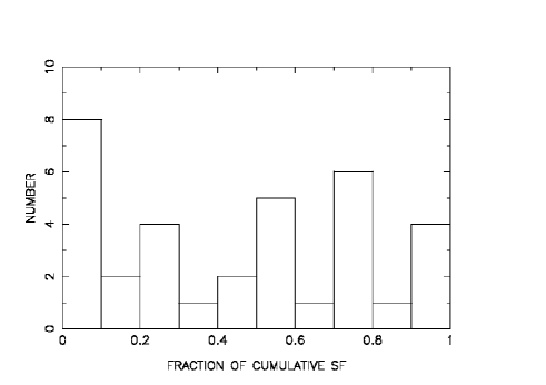
Figure 8: Histogram of the NCR values of the SN-containing pixels within the cumulative H$\alpha$ flux distribution of the 31 SNIc

4.3 SN ‘impostors’

The mean NCR value for the 6 SN ‘impostors’ is 0.105 (0.065), considerably lower than that of the SNII population. To measure the significance of this difference we used a Monte-Carlo analysis as for the SNIIb. We calculated the fraction of times that a mean NCR value of $\leq$0.105 (SN ‘impostors’ mean value) was produced when six values were drawn at random from the overall SNII NCR distribution. We found that there is a $\sim$10% chance that the SN ‘impostors’ are drawn from the same distribution as that of the SNII.

5 Discussion

There are two main discussion points that arise from the above results. The first is that there is a real excess seen in the number of SNII that do not appear to show any association to the H$\alpha$ emission, a result that was seen in JA06 and is backed up with the improved statistics presented within this paper. The second is the implications that differences in NCR values and distributions of the various CC SN types have on differences between their progenitor masses. If we assume that all stars originate within HII regions (the highest mass stars formed from an episode of SF will start to ionise the local hydrogen straight away), then the degree of association of each SN type with the overall emission can be used to constrain their relative stellar lifetimes (and therefore their relative initial masses), as with time, the stars will either move away from the host HII region due to their peculiar velocities, or the host HII region will cease to exist as the massive ionising stars will explode as the first set of SNe. Therefore we discuss the implications of our results for the different masses of the different CC types and how these implications fit with other results on the nature of the different SN progenitors.

5.1 An excess of SNII from regions of zero H$\alpha$ emission

The results presented in § 4.1 indicate that around $\sim$35% of SNII fall on sites of little or zero H$\alpha$ flux, compared to what would be expected if these SNe followed the underlying SF. For the SNIIP where we have 37 events in our sample this fractional excess remains the same. Recent research combining the results of a ten year survey for direct detections of SN progenitors (Smartt et al. 2008, in preparation; private communication) gives additional support to the growing evidence that CC SNe (SNIIP in particular) can arise from stars with initial masses of less than 10${\rm\ M}_{\odot}$. One of the main results from this survey is a lower mass value for producing SNIIP of 8.5${\rm\ M}_{\odot}$. Using the initial assumption for the current research that only stars with masses $>$10${\rm\ M}_{\odot}$ contribute significantly to producing H$\alpha$ emission we can then compare our statistics to this mass value. Assuming a Salpeter IMF and an upper mass limit for producing hydrogen rich CC SNe of 25${\rm\ M}_{\odot}$ (i.e. the upper mass limit for red supergiants; Levesque et al. 2007), we can calculate the range from 10${\rm\ M}_{\odot}$ downwards (in progenitor mass) that is consistent with our statistics of $\sim$35% of SNII falling on sites of little or zero H$\alpha$ emission. From these assumptions we calculate a lower mass value for producing SNII (and also the IIP sub-type) of 7.8${\rm\ M}_{\odot}$, consistent with that suggested by direct detections. Our results therefore seem to suggest that a significant fraction of SNII are produced by progenitor stars of less than 10${\rm\ M}_{\odot}$.
JA06 discussed alternative explanations to the fact that we find a significant fraction of SNII falling on sites of zero H$\alpha$ flux. These assumed that CC SNe arise from stars of initial mass $>$10${\rm\ M}_{\odot}$. Although as stated above there is growing evidence for the production of CC SNe from stars below 10${\rm\ M}_{\odot}$, the number of events used to make these constraints are still reasonably small and many stellar evolution codes predict CC from stars only of 10${\rm\ M}_{\odot}$ or higher (e.g. Ritossa et al. 1999). Here we therefore summarise a number of other physical processes that may be at play in producing the excess of SNII that we find occurring away from sites of recent SF.
In JA06 we discussed the ‘runaway’ hypothesis, that these SNe did originally form within an HII region but since moved to the position of the SN between stellar birth and death, due to some peculiar velocity. Another possibility is the destruction of massive clusters before the epoch of SN. Recent observations and simulations (Goodwin & Bastian, 2006; Bastian & Goodwin, 2006) have shown that many massive stellar clusters will in fact be destroyed on timescales of $\sim$10 Myr. Within the stellar cluster stars with the highest mass will explode as SNe first, thus exploding while the clusters are still stable and hence will be found to be associated with the H$\alpha$ emission produced from the ionisation of the local gas. These initial SNe (likely to be SNIc and Ib, see the next section) will drive the removal of gas from the cluster eventually leading to its destruction. Therefore within this scenario there are two possible processes that could lead to our result. Firstly with gas removal from the system it may be that there is little gas to be ionised and therefore no host HII region will be seen at the site of some SNII SNe. Secondly, as the cluster is destroyed while it attempts to regain virial equilibrium, many stars will be flung away with a high peculiar velocity leaving them far from their original host HII region.
Another explanation that was discussed in JA06 is the possibility that these SNe are occurring in regions of dust content, through which the SNe are visible but the H$\alpha$ emission is not. However, it is unclear why this would affect the SNII much more than the SNIb/c. It has also been found, through mid-IR observations of the SINGS survey, that highly obscured SF regions only seen in the IR make up only a small ($\sim$4%) fraction of the overall SF distribution in nearby galaxies (Prescott et al., 2007), arguing against this as a significant factor.

We conclude that the dominant effect producing our results on the association of SNII to the H$\alpha$ emission of their host galaxies is that a significant fraction of SNII progenitors are stars with initial masses below 10${\rm\ M}_{\odot}$. However, we also believe that it is likely that all the processes we discuss above play some part in producing the observed NCR distribution. We have discussed the various processes that could be involved in shaping the results that we see, now we will explore how we can use these results to compare and constrain the nature of the different progenitors of the different CC SN types.

5.2 Relative progenitor masses

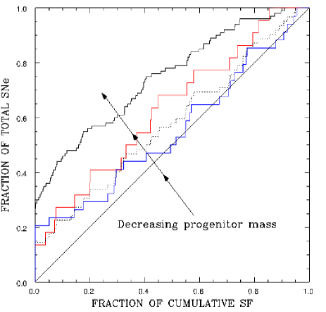
Figure 9: Cumulative distribution of the NCR values for the various CC sub-types: black represents the overall SNII population, red the SNIb, dotted the overall SNIb/c distribution and blue the SNIc. From comparing the distributions a sequence of decreasing progenitor mass emerges, indicated on the plot from the SNIc to Ib and finally the II showing the lowest degree of association to the line emission. The solid black diagonal line shows the expected results for a hypothetical population that exactly traces the H$\alpha$ line emission

From the arguments presented at the start of this section we can use comparisons of the mean NCR values of the different SN types to compare the relative mass ranges of their progenitors. The first conclusion is that we confirm the results of JA06 that overall the SNIb/c progenitor population arise from more massive progenitors than the SNII. When we compare the CC SN sub-types in detail we find that the different CC sub-types appear to form a sequence of increasing progenitor mass, going from SNII at the low mass end, through SNIb to SNIc as the highest mass progenitors. This sequence is illustrated in Fig. 9. In this figure we plot the cumulative distributions of the NCR values of the overall SNII, the SNIb/c, and the SNIb and Ic distributions individually. We also plot a hypothetical distribution for a population that exactly traces the line emission. The plot shows that the SNIc accurately traces the H$\alpha$ emission, except for a slight excess of NCR values at zero. As we go to the other SN distributions we see that they show an increasingly lower association to the line emission. A distinctive pattern emerges as indicated by the arrows on the plot, going from high to lower and lower mass progenitors implied from the differences between the distributions and the hypothetical flat distribution. This sequence can be seen to fit to the paradigm where CC SNe (II, Ib then Ic) arise from stars of increasingly higher initial mass, leading to stronger pre-SN stellar winds that strip the stars of their envelopes and produce the observed differences we see in their spectra.

With the statistics presented in §4 it is harder to make any firm statements as to differences within the progenitor masses of the various SNII sub-types. However, with the small number of SNIIL as a strong caveat, it seems that these SNe arise from similar mass progenitors to the SNIIP. This would imply that that metallicity or binarity may play a dominant role in deciding SN type, by enabling additional envelope stripping prior to explosion.
With respect to the SNIIb, although we only have 4 objects in our sample our results suggest that these SNe arise from more massive progenitors than the overall SNII population. They also show a higher degree of association to the H$\alpha$ emission than the SNIb (although again we stress the low statistics involved). A recent discovery of the progenitor of a IIb SN (Crockett et al., 2008) has suggested a possible progenitor mass of 28${\rm\ M}_{\odot}$, consistent with our result that these SNe arise from towards the high end of the CC SN progenitor sequence. The only other direct detection of a SNIIb progenitor is that of SN 1993J. Maund et al. (2004) estimated that this SN arose from a interacting binary with components of 14 and 15 ${\rm\ M}_{\odot}$ stars. Again our result that SNIIb arise from stars that follow the H$\alpha$ emission of their host galaxies is consistent with this result.
One of the most interesting results to arise from this work regards the SNIIn. Our results (see § 4.1.4) suggest that these SNe arise from similar mass progenitors to the overall SNII population and do not follow the underlying H$\alpha$ emission of their host galaxies. This would seem to be in conflict with recent thoughts on this SN type. Arguments have been put forward (e.g. Smith 2008 and references therein) that the observations of these SNe (strong narrow emission lines and high luminosities) require high pre-SN mass loss rates and huge circumstellar envelopes, arising from only the most massive stars, which would presumably trace the H$\alpha$ emission within galaxies. It has also been argued that two SNIIn, (2005gl and 2005gj) had luminous blue variable (LBV) progenitors (Gal-Yam et al. 2007; Trundle et al. 2008, respectively), again stars of very high mass ($\sim$25-40${\rm\ M}_{\odot}$ and above). Although some SNIIn probably do arise from very massive stars, our results suggest that the majority of these events arise from progenitors towards the low end of the CC progenitor mass range. A recent direct detection of the progenitor of the SNIIn 2008S on pre-explosion SPITZER mid-IR images (Prieto et al., 2008), enabled an estimate to be made of the progenitor mass of $\sim$10${\rm\ M}_{\odot}$ consistent with our results (however, there is some debate as to whether this is a true SN and it is unlike most other SNIIn; Smartt 2008, private communication). An intriguing possibility for progenitors from this mass range would be the super-AGB stars (SAGBs), a scenario suggested by the modeling of Poelarends et al. (2008). The initial mass range for SAGB evolution is 7.5-9.25${\rm\ M}_{\odot}$ and it is thought that the upper mass part of this range will produce electron-capture (EC) SNe (Poelarends et al., 2008). The mass-loss rates of these systems can be extremely high due to a large number of thermal pulses, potentially producing the capacity for interaction of the SN with a large amount of circumstellar material, and hence the narrow emission lines seen in SNIIn.
SN ‘impostors’ are thought to be the outbursts of very massive unstable LBV stars (van Dyk et al., 2000; Maund et al., 2006) that go through stages of intense mass loss, during which the luminosity of such objects can rise by more than three magnitudes (see Humphreys & Davidson 1994 for a review on this subject), hence masquerading as ‘true’ SNe. Given the presumed high mass nature of these events (and therefore their relatively short stellar lifetimes) one would expect these events to trace the distribution of high mass SF within their host galaxies. However, our results presented in § 4.3 would seem to be inconsistent with this picture. We find that the SN ‘impostors’ within our sample do not trace the underlying SF and in fact show the lowest degree of association of all SN types analysed in the current paper. We stress again here that there are only 6 such events within our sample and it is therefore hard to draw any firm conclusions before the statistics are improved. We note however that many LBVs observed in the local group are often more isolated than one would expect and are not always found within dense young stellar clusters (Burggraf et al., 2006).

6 Conclusions

We find that there is a significant fraction of the SNII population that do not show any association to the distribution of H$\alpha$ line emission. This excess of $\sim$35% of SNII falling on sites of little or zero H$\alpha$ flux, compared to what would be expected if they accurately traced the underlying SF, suggests that a large fraction of SNII arise from progenitor stars of less than 10${\rm\ M}_{\odot}$. Our results also imply that the different CC SN types can be separated into a sequence of increasing progenitor mass running from the SNII through the Ib, with finally the SNIc arising from the highest mass progenitors. We now summarise our findings on the possible relative mass ranges of the progenitors of the different CC SN types.

• Assuming that only stars of 10${\rm\ M}_{\odot}$ and above significantly contribute to the ionising flux that produces H$\alpha$ emission within galaxies, we calculate a lower mass limit for producing SNII of 7.8${\rm\ M}_{\odot}$.

• We confirm the results of JA06, that the SNIb/c trace the SF of their host galaxies more accurately than the SNII, implying that they arise from a higher mass progenitor population than the SNII.

• SNIc accurately trace the underlying SF within their host galaxies and therefore probably arise from the highest mass progenitors of all SNe.

• SNIIL show a similar degree of association to H$\alpha$ emission as the overall SNII population implying that they arise from stars of similar mass to those of SNIIP, with metallicity or binarity probably playing an important role in removing part of their envelopes and thus changing the shape of their light curves.

• Our results suggest that SNIIb arise from more massive stars than the overall SNII population.

• Although some SNIIn may arise from very massive stars, our results suggest that the majority come from the low end of the CC mass spectrum.

• SN ‘impostors’ do not seem to trace the high mass SF within host galaxies.

Appendix A Application of the Kolmogorov-Smirnov test to the SN data

In this appendix we highlight a feature of commonly-used implementations of the KS test, which caused particular problems for the analysis presented in this paper. These tests were implemented using the on-line statistics calculator at
http://www.physics.csbsju.edu/stats/KS-test.html
but identical results were found with a direct implementation of the kstwo code from ‘Numerical Recipes’ (Press et al., 1992).
The problems were noted when we initially found apparently significant differences between distributions of NCR values that to the eye appeared quite similar. The $D$ statistic, parametrising the maximum difference between pairs of normalised cumulative distributions, was for some tests found to be significantly over-estimated. It appears that this occurs for those distributions with significant numbers of points with identical values (which for our NCR distributions tend to be zeroes), and where the two samples are of different sizes. The sceptical reader can quickly test this, using the above website, and the following points as input:
0.01 0.23 0.32 0.40 0.40 0.40 0.40 0.51 0.59 0.63 0.67 0.73
Paste these numbers once into one of the data entry boxes, and twice into the other, to give samples with identical normalised cumulative distributions, but different overall sizes. This results in an estimated $D$ of 0.1667, in spite of the identical cumulative distributions. The overestimate of $D$ appears strongly dependent on the number of identical points (large ‘steps’ in the cumulative distribution), which are a particular feature of our datasets, but will certainly affect some other applications.
This does not appear to be a generally appreciated problem. We advocate careful checking of the $D$ value produced by KS software against an accurate plot of the normalised cumulative distributions, to ensure it is a real difference, and not an artefact caused by steps in the distributions.

Appendix B SN and host galaxy data

Table 1: Data for all SNe and host galaxies

SN	Host galaxy	Galaxy type	V${}_{\textit{r}}$ (kms-1)	SN type	NCR value	Telescope	Reference
1917A	NGC 6946	SABcd	48	II	0.207	INT
1921B	NGC 3184	SABcd	592	II	0.000	INT
1926A	NGC 4303	SABbc	1566	IIL	0.078	INT
1937F	NGC 3184	SABcd	592	IIP	0.000	INT
1940B	NGC 4725	SABab	1206	IIP	0.000	INT
1941A	NGC 4559	SABcd	816	IIL	0.859	INT
1941C	NGC 4136	SABc	609	II	0.000	JKT
1948B	NGC 6946	SABcd	48	IIP	0.387	INT
1954A	NGC 4214	IABm	291	Ib	0.000	INT
1954C	NGC 5879	SAc	772	II	0.163	JKT
1954J	NGC 2403	SABcd	131	‘impostor’*	0.187	INT	van Dyk et al. (2005)
1961I	NGC 4303	SABbc	1566	II	0.327	INT
1961V	NGC 1058	SABc	518	‘impostor’*	0.363	JKT	Goodrich et al. (1989)
1961U	NGC 3938	SABc	809	IIL	0.000	LT
1962L	NGC 1073	SABc	1208	Ic	0.000	JKT
1964A	NGC 3631	SABc	1156	II	0.000	INT
1964F	NGC 4303	SABbc	1566	II	0.000	INT
1964H	NGC 7292	IBm	986	II	0.059	JKT
1964L	NGC 3938	SABc	809	Ic	0.000	LT
1965H	NGC 4666	SABc	1529	IIP	0.597	LT
1965N	NGC 3074	SABc	5144	IIP	0.031	INT
1965L	NGC 3631	SABc	1156	IIP	0.001	INT
1966B	NGC 4688	SBcd	986	IIL	0.367	LT
1966J	NGC 3198	SBc	663	Ib	0.000	INT
1967H	NGC 4254	SAc	2407	II*	0.568	INT	van Dyk (1992)
1968D	NGC 6946	SABcd	48	II	0.018	INT
1968I	NGC 4254	SAc	2407	IIP	0.000	INT
1968V	NGC 2276	SABc	2410	II	0.327	JKT
1969B	NGC 3556	SBcd	699	IIP	0.191	INT
1969L	NGC 1058	SAc	518	IIP	0.000	JKT
1971S	NGC 493	SABcd	2338	IIP	0.174	JKT
1971K	NGC 3811	SBcd	3105	IIP	0.176	INT
1972Q	NGC 4254	SAc	2407	IIP	0.405	INT
1972R	NGC 2841	SAb	638	Ib	0.071	INT
1973R	NGC 3627	SABb	727	IIP	0.325	INT
1975T	NGC 3756	SABbc	1318	IIP	0.000	INT
1979C	NGC 4321	SABbc	1571	IIL	0.000	LT
1980K	NGC 6946	SABcd	48	IIL	0.007	INT
1982F	NGC 4490	SBd	565	IIP	0.095	INT
1983I	NGC 4051	SABbc	700	Ic	0.265	JKT
1984E	NGC 3169	SAa	1238	IIL	0.616	INT
1985G	NGC 4451	Sbc	864	IIP	0.641	INT
1985F	NGC 4618	SBm	544	Ib*	0.854	LT	Gaskell et al. (1986)
1985L	NGC 5033	SAc	875	IIL	0.301	INT
1987F	NGC 4615	Scd	4716	IIn	0.352	INT
1987K	NGC 4651	SAc	805	IIb	0.746	JKT
1987M	NGC 2715	SABc	1339	Ic	0.000	INT
1988L	NGC 5480	SAc	1856	Ib	0.425	LT
1989C	UGC 5249	SBd	1874	IIP	0.689	LT
1990E	NGC 1035	SAc	1241	IIP	0.000	LT
1990H	NGC 3294	SAc	1586	IIP*	0.000	INT	Filippenko (1993)
1990U	NGC 7479	SBc	2381	Ic	0.712	JKT
1991A	IC 2973	SBd	3210	Ic	0.773	INT
1991G	NGC 4088	SABbc	757	IIP	0.066	JKT
1991N	NGC 3310	SABbc	993	Ic	0.759	JKT
1992C	NGC 3367	SBc	3040	II	0.021	INT
1993G	NGC 3690	Double system	3121	IIL*	0.064	INT	Tsvetkov (1994)
1993X	NGC 2276	SABc	2410	II	0.039	JKT
1994I	NGC 5194	SAbc	463	Ic	0.550	INT
1994Y	NGC 5371	SABbc	2558	IIn	0.000	INT
1994ak	NGC 2782	SABa	2543	IIn	0.000	LT
1995F	NGC 2726	SABc	2410	Ic	0.548	JKT
1995N	MCG -02-38-17	IBm	1856	IIn	0.001	LT

Table 1: Data for all SNe and host galaxies

SN	Host galaxy	Galaxy type	V${}_{\textit{r}}$ (kms-1)	SN type	NCR value	Telescope	Reference
1995V	NGC 1087	SABc	1517	II	0.424	JKT
1995ag	UGC 11861	SABdm	1481	II	0.660	JKT
1996ae	NGC 5775	Sb	1681	IIn	0.747	JKT
1996ak	NGC 5021	SBb	8487	II	0.562	INT
1996aq	NGC 5584	SABcd	1638	Ic	0.050	LT
1996bu	NGC 3631	SAc	1156	IIn	0.000	INT
1997bs	NGC 3627	SABb	727	‘impostor’*	0.023	INT	van Dyk et al. (2000)
1997X	NGC 4691	SBO/a	1110	Ic	0.323	INT
1997db	UGC 11861	SABdm	1481	II	0.029	JKT
1997dn	NGC 3451	Sd	1334	II	0.073	JKT
1997dq	NGC 3810	SAc	993	Ic*	0.296	JKT	Mazzali et al. (2004)
1997eg	NGC 5012	SABc	2619	IIn	0.338	INT
1997ei	NGC 3963	SABbc	3188	Ic	0.288	INT
1998C	UGC 3825	SABbc	8281	II	0.000	INT
1998T	NGC 3690	Double system	3121	Ib	0.578	INT
1998Y	NGC 2415	Im?	3784	II	0.349	INT
1998cc	NGC 5172	SABbc	4030	Ib	0.331	INT
1999D	NGC 3690	Double system	3121	II	0.054	INT
1999br	NGC 4900	SBd	960	IIP*	0.099	JKT	Hamuy (2003)
1999bu	NGC 3786	SABa	2678	Ic	0.000	INT
1999bw	NGC 3198	SBc	663	‘impostor’*	0.000	INT	van Dyk et al. (2005)
1999dn	NGC 7714	SBb	2798	Ib	0.038	JKT
1999ec	NGC 2207	SABbc	2741	Ib	0.815	INT
1999ed	UGC 3555	SABbc	4835	II	0.615	INT
1999em	NGC 1637	SABc	717	IIP	0.394	LT
1999gb	NGC 2532	SABc	5260	IIn	0.676	INT
1999gi	NGC 3184	SABcd	592	IIP	0.637	INT
1999gn	NGC 4303	SABbc	1566	IIP*	0.897	INT	Pastorello et al. (2004)
2000C	NGC 2415	Im?	3784	Ic	0.494	INT
2000cr	NGC 5395	SAb	3491	Ic	0.000	INT
2000de	NGC 4384	Sa	2513	Ib	0.554	INT
2000ew	NGC 3810	SAc	993	Ic	0.907	JKT
2001B	IC 391	SAc	1556	Ib	0.201	INT
2001M	NGC 3240	SABb	3550	Ic	0.142	INT
2001R	NGC 5172	SABbc	4030	IIP*	0.000	INT	Matheson et al. (2001)
2001aa	UGC 10888	SBb	6149	II	0.000	INT
2001ac	NGC 3504	SABab	1534	‘impostor’*	0.000	INT	Matheson & Calkins (2001)
2001ai	NGC 5278	SAb	7541	Ic	0.878	INT
2001co	NGC 5559	SBb	5166	Ib/c	0.313	INT
2001ef	IC 381	SABbc	2476	Ic	0.944	INT
2001ej	UGC 3829	Sb	4031	Ib	0.314	INT
2001fv	NGC 3512	SABc	1376	IIP*	0.169	INT	Matheson et al. (2001)
2001gd	NGC 5033	SAc	875	IIb	0.459	INT
2001is	NGC 1961	SABc	3934	Ib	0.449	INT
2002A	UGC 3804	SABbc	2887	IIn	0.401	JKT
2002bm	MCG -01-32-19	SBbc	5462	Ic	0.565	INT
2002bu	NGC 4242	SABdm	506	IIn	0.000	JKT
2002ce	NGC 2604	SBcd	2078	II	0.108	JKT
2002cg	UGC 10415	SABb	9574	Ic	0.955	INT
2002cp	NGC 3074	SABc	5144	Ib/c	0.131	INT
2002cw	NGC 6700	SBc	4588	Ib	0.370	INT
2002dw	UGC 11376	S	6528	II	0.475	INT
2002ed	NGC 5468	SABcd	2842	IIP	0.395	INT
2002ei	MCG -01-09-24	Sab	2319	IIP	0.909	LT
2002fj	NGC 2596	Sb	5938	IIn	0.558	INT
2002gd	NGC 7537	SAbc	2674	II	0.167	JKT
2002hh	NGC 6946	SABcd	48	IIP	0.000	INT
2002hn	NGC 2532	SABc	5260	Ic	0.672	INT
2002ho	NGC 4210	SBb	2732	Ic	0.405	INT
2002ji	NGC 3655	SAc	1473	Ib/c	0.078	INT
2002jz	UGC 2984	SBdm	1543	Ic	0.513	INT
2002kg	NGC 2403	SABcd	131	‘impostor’*	0.055	INT	Maund et al. (2006)
2003H	NGC 2207	SABbc	2741	Ib	0.144	INT

Table 1: Data for all SNe and host galaxies

SN	Host galaxy	Galaxy type	V${}_{\textit{r}}$ (kms-1)	SN type	NCR value	Telescope	Reference
2003T	UGC 4864	SAab	8368	II	0.056	INT
2003Z	NGC 2742	SAc	1289	IIP*	0.013	JKT	Pastorello et al. (2004)
2003ab	UGC 4930	Scd	8750	II	0.000	INT
2003ao	NGC 2993	Sa	2430	IIP	0.157	LT
2003at	MCG +11-20-23	Sbc	7195	II	0.728	INT
2003bp	NGC 2596	Sb	5938	Ib	0.075	INT
2003db	MCG +05-23-21	S?	8113	II	0.150	INT
2003ed	NGC 5303	Pec	1419	IIb	0.554	LT
2003ef	NGC 4708	SAab	4166	II*	0.257	INT	Ganeshalingam et al. (2003)
2003el	NGC 5000	SBbc	5608	Ic	0.728	INT
2003hp	UGC 10942	SB	6378	Ic	0.000	INT
2003hr	NGC 2551	SAO/a	2344	II	0.000	JKT
2003ie	NGC 4051	SABbc	700	II	0.373	JKT
2003ig	UGC 2971	S	5881	Ic	0.769	INT
2004A	NGC 6207	SAc	852	IIP*	0.000	JKT	Hendry et al. (2006)
2004C	NGC 3683	SBc	1716	Ic	0.920	INT
2004G	NGC 5668	SAd	1582	II	0.000	INT
2004ao	UGC 10862	SBc	1691	Ib	0.420	INT
2004bm	NGC 3437	SABc	1283	Ic	0.704	INT
2004bs	NGC 3323	SB?	5164	Ib	0.200	INT
2004dg	NGC 5806	SABb	1359	IIP*	0.554	JKT	S. Smartt (2008, priv comm)
2004dk	NGC 6118	SAcd	1573	Ib	0.794	INT
2004ep	IC 2152	SABab	1875	II	0.289	LT
2004gq	NGC 1832	SBbc	1939	Ib	0.738	LT
2004gt	NGC 4038	SBm	1642	Ib/c	0.758	LT
2004ge	UGC 3555	SABbc	4835	Ic	0.293	INT
2005O	NGC 3340	S	5558	Ib	0.709	INT
2005V	NGC 2146	SBab	893	Ib/c	0.000	LT
2005ad	NGC 941	SABc	1608	IIP*	0.000	INT	S. Smartt (2008, priv comm)
2005ay	NGC 3938	SAc	809	IIP	0.873	LT
2005az	NGC 4961	SBcd	2535	Ic*	0.000	LT	Burket et al. (2005)
2005cs	NGC 5194	SAbc	463	IIP	0.396	INT
2005dl	NGC 2276	SABc	2410	II	0.730	INT
2005dp	NGC 5630	Sdm	2655	II	0.511	LT
2005kk	NGC 3323	SB?	5164	II	0.116	INT
2005kl	NGC 4369	SAa	1045	Ic	0.570	LT
2005lr	ESO 492-G2	SAb	2590	Ic	0.175	LT
2006am	NGC 5630	Sdm	2655	IIn	0.000	LT
2006gi	NGC 3147	SAbc	2820	Ib	0.000	INT
2006jc	UGC 4904	SB	1670	Ib/c	0.172	LT
2006ov	NGC 4303	SABbc	1566	IIP	0.284	INT
2008ax	NGC 4490	SBd	565	IIb	0.080	INT

Table 2: Data for all SNe and host galaxies: Columns 1 and 2 give the SN and host galaxy respectively. In columns 3 and 4 we present the morphological type and recession velocities of the host galaxies (both taken from NED). In column 5 the SN types are listed and the NCR data for each SN are given in column 6. In column 7 the telescope used for imaging of the SN host galaxy is given and for SNe where type classification was changed from those given in the Asiago catalogue a reference for the new designated type is given in the final column, and these type classifications are marked with an asterisk.

References

- Barbon et al. (1979) Barbon R., Ciatti F., Rosino L., 1979, A&A, 72, 287
- Bartunov et al. (1994) Bartunov O. S., Tsvetkov D. Y., Filimonova I. V., 1994, PASP, 106, 1276
- Bastian & Goodwin (2006) Bastian N., Goodwin S. P., 2006, MNRAS, 369, L9
- Burggraf et al. (2006) Burggraf B., Weis K., Bomans D. J., 2006, in Lamers H. J. G. L. M., Langer N., Nugis T., Annuk K., eds, Stellar Evolution at Low Metallicity: Mass Loss, Explosions, Cosmology Vol. 353 of Astronomical Society of the Pacific Conference Series, LBVs in M33: Their Environments and Ages. pp 245
- Burket et al. (2005) Burket J., Pugh H., Li W., Puckett T., Cox L., 2005, IAUC CBET, 8504, 2
- Chugai & Danziger (1994) Chugai N. N., Danziger I. J., 1994, MNRAS, 268, 173
- Crockett et al. (2008) Crockett R. M., et al., 2008, ArXiv e-prints, 805
- Eldridge et al. (2008) Eldridge J. J., Izzard R. G., Tout C. A., 2008, MNRAS, 384, 1109
- Eldridge & Tout (2004) Eldridge J. J., Tout C. A., 2004, MNRAS, 353, 87
- Filippenko (1993) Filippenko A. V., 1993, in Bulletin of the American Astronomical Society Vol. 25 of Bulletin of the American Astronomical Society, The Spectroscopic and Photometric Evolution of Type II Supernovae. pp 819
- Filippenko et al. (1993) Filippenko A. V., Matheson T., Ho L. C., 1993, ApJ Let., 415, L103
- Gal-Yam et al. (2007) Gal-Yam A., et al., 2007, ApJ, 656, 372
- Ganeshalingam et al. (2003) Ganeshalingam M., Graham J., Pugh H., Li W., 2003, IAUC CBET, 8134, 1
- Gaskell et al. (1986) Gaskell C. M., Cappellaro E., Dinerstein H. L., Garnett D. R., Harkness R. P., Wheeler J. C., 1986, ApJ Let., 306, L77
- Goodrich et al. (1989) Goodrich R. W., Stringfellow G. S., Penrod G. D., Filippenko A. V., 1989, ApJ, 342, 908
- Goodwin & Bastian (2006) Goodwin S. P., Bastian N., 2006, MNRAS, 373, 752
- Hamuy (2003) Hamuy M., 2003, ApJ, 582, 905
- Heger et al. (2003) Heger A., Fryer C. L., Woosley S. E., Langer N., Hartmann D. H., 2003, ApJ, 591, 288
- Hendry et al. (2006) Hendry M. A., et al., 2006, MNRAS, 369, 1303
- Hoyle & Fowler (1960) Hoyle F., Fowler W. A., 1960, ApJ, 132, 565
- Humphreys & Davidson (1994) Humphreys R. M., Davidson K., 1994, PASP, 106, 1025
- James & Anderson (2006) James P. A., Anderson J. P., 2006, A&A, 453, 57
- James et al. (2004) James P. A., et al., 2004, A&A, 414, 23
- Kennicutt (1998) Kennicutt Jr. R. C., 1998, ARA&A, 36, 189
- Kobulnicky & Fryer (2007) Kobulnicky H. A., Fryer C. L., 2007, ApJ, 670, 747
- Kudritzki & Puls (2000) Kudritzki R.-P., Puls J., 2000, ARA&A, 38, 613
- Levesque et al. (2007) Levesque E. M., Massey P., Olsen K. A. G., Plez B., 2007, ApJ, 667, 202
- Li et al. (2006) Li W., Van Dyk S. D., Filippenko A. V., Cuillandre J.-C., Jha S., Bloom J. S., Riess A. G., Livio M., 2006, ApJ, 641, 1060
- Li et al. (2007) Li W., Wang X., Van Dyk S. D., Cuillandre J.-C., Foley R. J., Filippenko A. V., 2007, ApJ, 661, 1013
- Matheson & Calkins (2001) Matheson T., Calkins M., 2001, IAUC CBET, 7597, 3
- Matheson et al. (2001) Matheson T., Jha S., Challis P., Kirshner R., Berlind P., 2001, IAUC CBET, 7756, 4
- Matheson et al. (2001) Matheson T., Jha S., Challis P., Kirshner R., Calkins M., 2001, IAUC CBET, 7583, 2
- Maund et al. (2006) Maund J. R., et al., 2006, MNRAS, 369, 390
- Maund et al. (2005) Maund J. R., Smartt S. J., Danziger I. J., 2005, MNRAS, 364, L33
- Maund et al. (2004) Maund J. R., Smartt S. J., Kudritzki R. P., Podsiadlowski P., Gilmore G. F., 2004, Nature, 427, 129
- Mazzali et al. (2004) Mazzali P. A., Deng J., Maeda K., Nomoto K., Filippenko A. V., Matheson T., 2004, ApJ, 614, 858
- Mokiem et al. (2007) Mokiem M. R., et al., 2007, A&A, 473, 603
- Nomoto et al. (1993) Nomoto K., Suzuki T., Shigeyama T., Kumagai S., Yamaoka H., Saio H., 1993, Nature, 364, 507
- Pastorello et al. (2004) Pastorello A., et al., 2004, MNRAS, 347, 74
- Podsiadlowski et al. (1993) Podsiadlowski P., Hsu J. J. L., Joss P. C., Ross R. R., 1993, Nature, 364, 509
- Podsiadlowski et al. (1992) Podsiadlowski P., Joss P. C., Hsu J. J. L., 1992, ApJ, 391, 246
- Podsiadlowski et al. (1990) Podsiadlowski P., Joss P. C., Rappaport S., 1990, A&A, 227, L9
- Poelarends et al. (2008) Poelarends A. J. T., Herwig F., Langer N., Heger A., 2008, ApJ, 675, 614
- Prescott et al. (2007) Prescott M. K. M., et al., 2007, ApJ, 668, 182
- Press et al. (1992) Press W. H., Teukolsky S. A., Vetterling W. T., Flannery B. P., 1992, Numerical recipes in FORTRAN. The art of scientific computing. Cambridge: University Press, —c1992, 2nd ed.
- Prieto et al. (2008) Prieto J. L., et al., 2008, ApJ Let., 681, L9
- Puls et al. (1996) Puls J., et al., 1996, A&A, 305, 171
- Ritossa et al. (1999) Ritossa C., García-Berro E., Iben I. J., 1999, ApJ, 515, 381
- Schlegel (1990) Schlegel E. M., 1990, MNRAS, 244, 269
- Shigeyama et al. (1990) Shigeyama T., Nomoto K., Tsujimoto T., Hashimoto M.-A., 1990, ApJ Let., 361, L23
- Smartt et al. (2004) Smartt S. J., Maund J. R., Hendry M. A., Tout C. A., Gilmore G. F., Mattila S., Benn C. R., 2004, Science, 303, 499
- Smith (2008) Smith N., 2008, in IAU Symposium Vol. 250 of IAU Symposium, Episodic Mass Loss and Pre-SN Circumstellar Envelopes. pp 193–200
- Steele et al. (2004) Steele I. A., et al., 2004, in Oschmann Jr. J. M., ed., Ground-based Telescopes. Edited by Oschmann, Jacobus M., Jr. Proceedings of the SPIE, Volume 5489, pp. 679-692 (2004). Vol. 5489 of Presented at the Society of Photo-Optical Instrumentation Engineers (SPIE) Conference, The Liverpool Telescope: performance and first results. pp 679–692
- Trundle et al. (2008) Trundle C., Kotak R., Vink J. S., Meikle W. P. S., 2008, ArXiv e-prints, 804
- Tsvetkov (1994) Tsvetkov D. Y., 1994, Astronomy Letters, 20, 374
- van den Bergh et al. (2002) van den Bergh S., Li W., Filippenko A. V., 2002, PASP, 114, 820
- van Dyk (1992) van Dyk S. D., 1992, AJ, 103, 1788
- van Dyk et al. (2005) van Dyk S. D., Filippenko A. V., Chornock R., Li W., Challis P. M., 2005, PASP, 117, 553
- van Dyk et al. (1996) van Dyk S. D., Hamuy M., Filippenko A. V., 1996, AJ, 111, 2017
- van Dyk et al. (2000) van Dyk S. D., Peng C. Y., King J. Y., Filippenko A. V., Treffers R. R., Li W., Richmond M. W., 2000, PASP, 112, 1532